


1 Introduction
Understanding the behaviour and propagation of plasma waves is of fundamental importance in both laboratory and space plasmas. In laboratory plasmas, waves are a naturally occurring phenomena that arise due to various mechanisms, such as via superthermal energetic particles in tokamaks (Heidbrink Reference Heidbrink2008), although they can also be deliberately excited via external circuitry. There are many reasons one would want to excite plasma waves in a laboratory environment, although the two most common applications are for the purposes of plasma heating and diagnostics. As the exceedingly high energy densities found in the core of burning tokamak plasmas prevent direct diagnostic measurements, many fusion diagnostic tools rely on exciting waves along the edge of the plasma, and then inferring the various physical properties of the plasma from the resulting wave propagation. Some examples of this include laser interferometry (Baker & Lee Reference Baker and Lee1978) and Doppler reflectometry (Hirsch et al. Reference Hirsch, Holzhauer, Baldzuhn, Kurzan and Scott2001). The predictive capability of antenna-based diagnostics is only as good as our understanding of the underlying physics, as well as our ability to effectively and accurately recreate the measured results in a simulated environment.
In general, plasma antennae fall into two major categories: those in direct electrical contact with the plasma, and those which rely on indirect (i.e. inductive or capacitive) coupling. Alfvén waves excited by direct coupling have been explored in great detail in the large plasma device (LAPD) at UCLA (Gekelman et al. Reference Gekelman, Pribyl, Lucky, Drandell, Leneman, Maggs, Vincena, Compernolle, Tripathi and Morales2016), and was in fact one of the original motivations for the machine being built (Gekelman et al. Reference Gekelman, Pfister, Lucky, Bamber, Leneman and Maggs1991). Early studies of shear (or slow) Alfvén waves used a small metal disk in order to drive plasma current and excite waves (Gekelman et al. Reference Gekelman, Vincena, Leneman and Maggs1994). In the inertial (cold) regime, the resulting wave front was observed to emanate from the disk in a narrow conical pattern, mediated by electrons in the parallel direction and a smaller ion polarization current across the background field (Gekelman et al. Reference Gekelman, Vincena, Leneman and Maggs1999). A theoretical companion paper, published around the same time, developed an analytic model for determining the spatial structure of inertial Alfvén waves launched by a metal disk exciter, and the predicted results were found to be in good agreement with experimental measurements (Morales, Loritsch & Maggs Reference Morales, Loritsch and Maggs1994). Similar experiments were later done in the kinetic regime using the same antenna (Gekelman et al. Reference Gekelman, Vincena, Leneman and Maggs1997), and the corresponding theoretical paper again agreed with the results (Morales & Maggs Reference Morales and Maggs1997). Both theoretical models take the general solution to the azimuthally symmetric cold plasma wave equation, and then use the boundary conditions imposed by the antenna (which can either be an equipotential or constant current surface) to uniquely determine the resulting spatial structure of the excited wave. While this methodology is successful for many simple antenna geometries, a generalization to this approach is desired for antennae which cannot be easily mapped to a set of straightforward boundary conditions.
Alfvén waves launched by inductively coupled antennae have also been studied in detail, in both the laboratory as well as in simulations. The rotating magnetic field (RMF) antenna, originally designed to study circularly polarized waves, consists of two orthogonal loops of current-carrying wire (Gigliotti et al. Reference Gigliotti, Gekelman, Pribyl, Vincena, Karavaev, Shao, Sharma and Papadopoulos2009). Experimental results showed that the RMF antenna excited large parallel electron currents where the antenna’s vacuum electric field pointed along the background field. Three-dimensional simulations of the RMF antenna were performed, which used a linear two-fluid magnetohydrodynamic (MHD) spectral model, and the results were in good agreement with experiment (Karavaev et al. Reference Karavaev, Gumerov, Papadopoulos, Shao, Sharma, Gekelman, Wang, Compernolle, Pribyl and Vincena2011). A similar semi-analytical model for analysing inductively coupled waves was previously devised by Jaeger et al. (Reference Jaeger, Berry, Tolliver and Batchelor1995) and used to model the behaviour of radio frequency (RF) power deposition in high-density plasma tools. Both of these theoretical models for inductively coupled antennae are similar in that they treat the external antenna currents as a ‘source’ term to the cold plasma wave equation, which is contrary to the strategy of boundary condition matching that was employed for the electrostatic disk exciter.
A vast array of numerical tools exists for simulating the behaviour of plasma waves launched by various antennae. Many tokamak plasmas are adequately described by a single fluid MHD model, and so several ray tracing codes exist to map out wave propagation in this simple regime (Smirnov Reference Smirnov2003). On the other end of the complexity spectrum, finite element (Glasser et al. Reference Glasser, Sovinec, Nebel, Gianakon, Plimpton, Chu and Schnak1999) and full-wave (Hillesheim et al. Reference Hillesheim, Holland, Schmitz, Kubota, Rhodes and Carter2012) models divide space and time up into a discrete grid (or mesh), and solve Maxwell’s equations incrementally to find the full spatial structure of the field. While these sorts of calculations are generally very accurate, they can also be extremely computationally expensive, and for simpler plasma systems a more semi-analytical approach may be advantageous. Unfortunately, in many situations where spatial inhomogeneities of the plasma are present and expected to play a large role in wave coupling, such numerical methods may be necessary for yielding accurate results. The ALOHA code (Hillairet et al. Reference Hillairet, Voyer, Ekedahl, Goniche, Kazda, Meneghini, Milanesio and Preynas2010) is an example of a full-wave simulation tool which was developed to model the coupling of lower hybrid waves to a cold, inhomogeneous plasma, such as those found in the scrape-off layer of tokamak plasmas. An example of a model which handles wave propagation in non-uniform plasmas while retaining a degree of analyticity is given by Chen & Arnush (Reference Chen and Arnush1997) and Arnush & Chen (Reference Arnush and Chen1998), and was developed to study helicon waves in cylindrical plasmas.
In this paper we present a robust semi-analytic model for modelling antenna-driven waves in a cold, uniform plasma. A semi-analytic model has the benefit of rewarding the user with reduced computation time in exchange for being able to solve any of the steps analytically, as well as granting physical insight into the problem that otherwise might not be evident with other numerical solvers. In order to simplify the problem, we will consider antennae which are current driven by external electronics, meaning any induced fields (either by the active elements of the antenna or the nearby plasma response) have no effect on the antenna currents. In practice, complex antennae will often have passive elements containing induced currents, in addition to the actively driven antenna current, and the total radiated field is then due to the contribution from both current types. The simulation code TOPICA (Milanesio et al. Reference Milanesio, Meneghini, Lancellotti, Maggiora and Vecchi2009), originally developed to establish predictive capability in ion cyclotron radio frequency (ICRF) heating schemes, is able to account for details in the antenna such as geometry, housing and shielding, as well as the induced currents within the passive antenna structures and their resulting radiated fields.
The remainder of the paper is organized as follows. In § 2 we derive the antenna wave equation, which is a system of partial differential equations that describes the plasma field excited by an indirectly coupled antenna, and then derive a simplified version for the case of an azimuthally symmetric antenna. In § 3 we find the general solution to the antenna wave equation, expressed as an integral over the vacuum field of the antenna. In § 4 we solve the general solution for the case of an electric dipole antenna of length
 $\ell$
, aligned along the background magnetic field, and discuss the resulting radiation (and near-field) behaviour. In § 5, we forgo all symmetry constraints and find the fully generalized solution to the antenna wave equation in Cartesian coordinates. Finally, in § 6 we offer some concluding remarks, including a discussion of the key physical insights gained from this analytic study as well as the advantages of this model in the context of simulations/numerical analysis.
$\ell$
, aligned along the background magnetic field, and discuss the resulting radiation (and near-field) behaviour. In § 5, we forgo all symmetry constraints and find the fully generalized solution to the antenna wave equation in Cartesian coordinates. Finally, in § 6 we offer some concluding remarks, including a discussion of the key physical insights gained from this analytic study as well as the advantages of this model in the context of simulations/numerical analysis.
2 Derivation of the antenna wave equation
Consider an electrically insulated antenna immersed in a cold, magnetized plasma, with background field
 $\boldsymbol{B}_{0}=B_{0}\hat{z}$
, which is driven by external circuitry at frequency
$\boldsymbol{B}_{0}=B_{0}\hat{z}$
, which is driven by external circuitry at frequency
 $\unicode[STIX]{x1D714}$
. We will assume the plasma to be infinite and unbounded. The combination of Ampere’s and Faraday’s laws gives us the following expression:
$\unicode[STIX]{x1D714}$
. We will assume the plasma to be infinite and unbounded. The combination of Ampere’s and Faraday’s laws gives us the following expression:
 $$\begin{eqnarray}\unicode[STIX]{x1D735}\times \left(\unicode[STIX]{x1D735}\times \boldsymbol{E}\right)=\text{i}\unicode[STIX]{x1D714}\unicode[STIX]{x1D707}_{0}\boldsymbol{J}_{pl}+\text{i}\unicode[STIX]{x1D714}\unicode[STIX]{x1D707}_{0}\boldsymbol{J}_{\text{ext}}+{\displaystyle \frac{\unicode[STIX]{x1D714}^{2}}{c^{2}}}\boldsymbol{E}.\end{eqnarray}$$
Note that we have adopted the sign convention
 $\unicode[STIX]{x2202}_{t}\rightarrow -\text{i}\unicode[STIX]{x1D714}$
. In (2.1),
$\unicode[STIX]{x2202}_{t}\rightarrow -\text{i}\unicode[STIX]{x1D714}$
. In (2.1),
 $\boldsymbol{J}_{\text{ext}}$
is the externally driven antenna current, and
$\boldsymbol{J}_{\text{ext}}$
is the externally driven antenna current, and
 $\boldsymbol{J}_{pl}$
is the plasma current. For positions within the plasma, we will assume the current density is related to the local electric field by a conductivity tensor, i.e.
$\boldsymbol{J}_{pl}$
is the plasma current. For positions within the plasma, we will assume the current density is related to the local electric field by a conductivity tensor, i.e.
 $\boldsymbol{J}_{pl}=\overset{\leftrightarrow }{\unicode[STIX]{x1D70E}}\boldsymbol{\cdot }\boldsymbol{E}$
. Additionally, the electric field can be redefined as
$\boldsymbol{J}_{pl}=\overset{\leftrightarrow }{\unicode[STIX]{x1D70E}}\boldsymbol{\cdot }\boldsymbol{E}$
. Additionally, the electric field can be redefined as
 $\boldsymbol{E}=\boldsymbol{E}_{0}+\boldsymbol{E}_{pl}$
, where
$\boldsymbol{E}=\boldsymbol{E}_{0}+\boldsymbol{E}_{pl}$
, where
 $\boldsymbol{E}_{0}$
is the vacuum electric field of the antenna and
$\boldsymbol{E}_{0}$
is the vacuum electric field of the antenna and
 $\boldsymbol{E}_{pl}$
is the rest of the field, which can be thought of as the plasma’s response to the antenna. Inserting these assumptions into (2.1) gives the following:
$\boldsymbol{E}_{pl}$
is the rest of the field, which can be thought of as the plasma’s response to the antenna. Inserting these assumptions into (2.1) gives the following:
 $$\begin{eqnarray}\unicode[STIX]{x1D735}\times \unicode[STIX]{x1D735}\times \boldsymbol{E}_{pl}+\unicode[STIX]{x1D735}\times \unicode[STIX]{x1D735}\times \boldsymbol{E}_{0}=\text{i}\unicode[STIX]{x1D714}\unicode[STIX]{x1D707}_{0}\overset{\leftrightarrow }{\unicode[STIX]{x1D70E}}\boldsymbol{\cdot }(\boldsymbol{E}_{pl}+\boldsymbol{E}_{0})+\text{i}\unicode[STIX]{x1D714}\unicode[STIX]{x1D707}_{0}\boldsymbol{J}_{\text{ext}}+{\displaystyle \frac{\unicode[STIX]{x1D714}^{2}}{c^{2}}}\boldsymbol{E}_{pl}+{\displaystyle \frac{\unicode[STIX]{x1D714}^{2}}{c^{2}}}\boldsymbol{E}_{0}.\end{eqnarray}$$
Subtracting out the vacuum wave equation, given by
 $\unicode[STIX]{x1D735}\times \unicode[STIX]{x1D735}\times \boldsymbol{E}_{0}=\text{i}\unicode[STIX]{x1D714}\unicode[STIX]{x1D707}_{0}\boldsymbol{J}_{\text{ext}}+(\unicode[STIX]{x1D714}^{2}/c^{2})\boldsymbol{E}_{0}$
, and defining the plasma dielectric tensor as
$\unicode[STIX]{x1D735}\times \unicode[STIX]{x1D735}\times \boldsymbol{E}_{0}=\text{i}\unicode[STIX]{x1D714}\unicode[STIX]{x1D707}_{0}\boldsymbol{J}_{\text{ext}}+(\unicode[STIX]{x1D714}^{2}/c^{2})\boldsymbol{E}_{0}$
, and defining the plasma dielectric tensor as
 $\overset{\leftrightarrow }{\unicode[STIX]{x1D700}}=\overset{\leftrightarrow }{I}+(\text{i}\unicode[STIX]{x1D700}_{0}\unicode[STIX]{x1D714})\overset{\leftrightarrow }{\unicode[STIX]{x1D70E}}$
allows us to express equation (2.2) in the following form:
$\overset{\leftrightarrow }{\unicode[STIX]{x1D700}}=\overset{\leftrightarrow }{I}+(\text{i}\unicode[STIX]{x1D700}_{0}\unicode[STIX]{x1D714})\overset{\leftrightarrow }{\unicode[STIX]{x1D70E}}$
allows us to express equation (2.2) in the following form:
 $$\begin{eqnarray}\unicode[STIX]{x1D735}\times \left(\unicode[STIX]{x1D735}\times \boldsymbol{E}_{pl}\right)-{\displaystyle \frac{\unicode[STIX]{x1D714}^{2}}{c^{2}}}\overset{\leftrightarrow }{\unicode[STIX]{x1D700}}\boldsymbol{\cdot }\boldsymbol{E}_{pl}=\text{i}\unicode[STIX]{x1D707}_{0}\unicode[STIX]{x1D714}\overset{\leftrightarrow }{\unicode[STIX]{x1D70E}}\boldsymbol{\cdot }\boldsymbol{E}_{0}.\end{eqnarray}$$
For a cold, strongly magnetized plasma, the dielectric tensor is given in cylindrical coordinates by the following (Stix Reference Stix1962):
 $$\begin{eqnarray}\left.\begin{array}{@{}c@{}}\overset{\leftrightarrow }{\unicode[STIX]{x1D700}}\boldsymbol{\cdot }\boldsymbol{E}=\left[\begin{array}{@{}ccc@{}}S & -\text{i}D & 0\\ \text{i}D & S & 0\\ 0 & 0 & P\\ \end{array}\right]\boldsymbol{\cdot }\left(\begin{array}{@{}c@{}}E_{r}\\ E_{\unicode[STIX]{x1D703}}\\ E_{z}\end{array}\right),\quad \begin{array}{@{}c@{}}S=1-\mathop{\sum }_{s}{\displaystyle \frac{\unicode[STIX]{x1D714}_{ps}^{2}}{\unicode[STIX]{x1D714}^{2}-\unicode[STIX]{x1D6FA}_{s}^{2}}},\\[10.0pt] D=\mathop{\sum }_{s}{\displaystyle \frac{\unicode[STIX]{x1D6FA}_{s}}{\unicode[STIX]{x1D714}}}{\displaystyle \frac{\unicode[STIX]{x1D714}_{ps}^{2}}{\unicode[STIX]{x1D714}^{2}-\unicode[STIX]{x1D6FA}_{s}^{2}}},\\[10.0pt] P=1-\mathop{\sum }_{s}{\displaystyle \frac{\unicode[STIX]{x1D714}_{ps}^{2}}{\unicode[STIX]{x1D714}(\unicode[STIX]{x1D714}+\text{i}\unicode[STIX]{x1D708}_{e})}},\end{array}\end{array}\right\}\end{eqnarray}$$
where the summations are over all particle species. In (2.4),
 $\unicode[STIX]{x1D714}_{ps}$
and
$\unicode[STIX]{x1D714}_{ps}$
and
 $\unicode[STIX]{x1D6FA}_{cs}$
are the plasma and cyclotron frequencies, respectively, and
$\unicode[STIX]{x1D6FA}_{cs}$
are the plasma and cyclotron frequencies, respectively, and
 $\unicode[STIX]{x1D708}_{e}$
is the total electron collision frequency. Note that the dielectric tensor defined by (2.4) is only valid for a plasma with background field
$\unicode[STIX]{x1D708}_{e}$
is the total electron collision frequency. Note that the dielectric tensor defined by (2.4) is only valid for a plasma with background field
 $\boldsymbol{B}_{0}=B_{0}\hat{z}$
pointing entirely in the
$\boldsymbol{B}_{0}=B_{0}\hat{z}$
pointing entirely in the
 $z$
direction, and is not valid when an azimuthal component of the background field is present (analogous to the background poloidal field commonly found in tokamaks). Equation (2.3) contains, in principle, all the information required to determine the field due to an antenna in the plasma. In the absence of an antenna, the right hand side of (2.3) goes to zero and the resulting differential equation is the cold plasma wave equation, whose solution gives all the wave-like modes predicted by the cold plasma model. The general solution to the cold plasma wave equation in cylindrical coordinates has been calculated before (Ram & Hizanidis Reference Ram and Hizanidis2016), in the context of the scattering of RF plane waves due to a cylindrical density filament. The right-hand side of (2.3) can be thought of as a ‘source’ term to the cold plasma wave equation, and is physically interpreted as the vacuum field coupling to the plasma conductivity to excite plasma currents. This is consistent with previous observations of Alfvén waves in the laboratory. Waves launched by a magnetic dipole antenna, lying in the
$z$
direction, and is not valid when an azimuthal component of the background field is present (analogous to the background poloidal field commonly found in tokamaks). Equation (2.3) contains, in principle, all the information required to determine the field due to an antenna in the plasma. In the absence of an antenna, the right hand side of (2.3) goes to zero and the resulting differential equation is the cold plasma wave equation, whose solution gives all the wave-like modes predicted by the cold plasma model. The general solution to the cold plasma wave equation in cylindrical coordinates has been calculated before (Ram & Hizanidis Reference Ram and Hizanidis2016), in the context of the scattering of RF plane waves due to a cylindrical density filament. The right-hand side of (2.3) can be thought of as a ‘source’ term to the cold plasma wave equation, and is physically interpreted as the vacuum field coupling to the plasma conductivity to excite plasma currents. This is consistent with previous observations of Alfvén waves in the laboratory. Waves launched by a magnetic dipole antenna, lying in the
 $XZ$
plane, were shown to induce two antiparallel current channels on either end of the dipole, where the vacuum electric field points in
$XZ$
plane, were shown to induce two antiparallel current channels on either end of the dipole, where the vacuum electric field points in
 $\pm \hat{z}$
(Gigliotti et al.
Reference Gigliotti, Gekelman, Pribyl, Vincena, Karavaev, Shao, Sharma and Papadopoulos2009). It is speculated that cross-field currents are also excited in front of the antenna, where the vacuum field points in
$\pm \hat{z}$
(Gigliotti et al.
Reference Gigliotti, Gekelman, Pribyl, Vincena, Karavaev, Shao, Sharma and Papadopoulos2009). It is speculated that cross-field currents are also excited in front of the antenna, where the vacuum field points in
 $\hat{x}$
, although for antennae of that scale they are generally much smaller than the induced parallel electron currents.
$\hat{x}$
, although for antennae of that scale they are generally much smaller than the induced parallel electron currents.
The cold plasma assumption allows us to solve (2.3) in configuration space, as the dielectric tensor is not a function of the wave vector
 $\boldsymbol{k}$
. For simplicity we will consider an antenna possessing azimuthal symmetry in cylindrical coordinates, although the general Cartesian solution is derived in § 5. The plasma response field excited by an azimuthally symmetric antenna is assumed to have the following form:
$\boldsymbol{k}$
. For simplicity we will consider an antenna possessing azimuthal symmetry in cylindrical coordinates, although the general Cartesian solution is derived in § 5. The plasma response field excited by an azimuthally symmetric antenna is assumed to have the following form:
 $$\begin{eqnarray}\boldsymbol{E}_{pl}={\textstyle \frac{1}{2}}[E_{r}(r,z,\unicode[STIX]{x1D714})\hat{r}+E_{\unicode[STIX]{x1D703}}(r,z,\unicode[STIX]{x1D714})\hat{\unicode[STIX]{x1D703}}+E_{z}(r,z,\unicode[STIX]{x1D714})\hat{z}]\text{e}^{-\text{i}\unicode[STIX]{x1D714}t}+\text{c.c.}\end{eqnarray}$$
Equation (2.3) can then be expanded out in cylindrical coordinates to give the following system of equations:
 $$\begin{eqnarray}\displaystyle \hspace{-24.0pt} & \displaystyle -{\displaystyle \frac{\unicode[STIX]{x2202}}{\unicode[STIX]{x2202}z}}\left({\displaystyle \frac{\unicode[STIX]{x2202}E_{r}}{\unicode[STIX]{x2202}z}}-{\displaystyle \frac{\unicode[STIX]{x2202}E_{z}}{\unicode[STIX]{x2202}r}}\right)-{\displaystyle \frac{\unicode[STIX]{x1D714}^{2}}{c^{2}}}SE_{r}+{\displaystyle \frac{\unicode[STIX]{x1D714}^{2}}{c^{2}}}\text{i}DE_{\unicode[STIX]{x1D703}}={\displaystyle \frac{\unicode[STIX]{x1D714}^{2}}{c^{2}}}(S-1)E_{r0}-{\displaystyle \frac{\unicode[STIX]{x1D714}^{2}}{c^{2}}}\text{i}DE_{\unicode[STIX]{x1D703}0}, & \displaystyle\end{eqnarray}$$
 $$\begin{eqnarray}\displaystyle \hspace{-24.0pt} & \displaystyle -{\displaystyle \frac{\unicode[STIX]{x2202}^{2}E_{\unicode[STIX]{x1D703}}}{\unicode[STIX]{x2202}z^{2}}}-{\displaystyle \frac{\unicode[STIX]{x2202}}{\unicode[STIX]{x2202}r}}\left({\displaystyle \frac{1}{r}}{\displaystyle \frac{\unicode[STIX]{x2202}}{\unicode[STIX]{x2202}r}}\left(rE_{\unicode[STIX]{x1D703}}\right)\right)-{\displaystyle \frac{\unicode[STIX]{x1D714}^{2}}{c^{2}}}\text{i}DE_{r}-{\displaystyle \frac{\unicode[STIX]{x1D714}^{2}}{c^{2}}}SE_{\unicode[STIX]{x1D703}}={\displaystyle \frac{\unicode[STIX]{x1D714}^{2}}{c^{2}}}\text{i}DE_{r0}+{\displaystyle \frac{\unicode[STIX]{x1D714}^{2}}{c^{2}}}(S-1)E_{\unicode[STIX]{x1D703}0}, & \displaystyle\end{eqnarray}$$
 $$\begin{eqnarray}\displaystyle \hspace{-24.0pt} & \displaystyle {\displaystyle \frac{1}{r}}{\displaystyle \frac{\unicode[STIX]{x2202}}{\unicode[STIX]{x2202}r}}\left(r{\displaystyle \frac{\unicode[STIX]{x2202}E_{r}}{\unicode[STIX]{x2202}z}}-r{\displaystyle \frac{\unicode[STIX]{x2202}E_{z}}{\unicode[STIX]{x2202}r}}\right)-{\displaystyle \frac{\unicode[STIX]{x1D714}^{2}}{c^{2}}}PE_{z}={\displaystyle \frac{\unicode[STIX]{x1D714}^{2}}{c^{2}}}(P-1)E_{z0}. & \displaystyle\end{eqnarray}$$
Note that we have dropped the
 $\text{pl}$
subscript on the plasma response term
$\text{pl}$
subscript on the plasma response term
 $\boldsymbol{E}_{\text{pl}}$
for brevity. Equations (2.6)–(2.8) can be reduced down to two differential equations if we recast it in terms of the azimuthal and radial magnetic field, given by Faraday’s law to be
$\boldsymbol{E}_{\text{pl}}$
for brevity. Equations (2.6)–(2.8) can be reduced down to two differential equations if we recast it in terms of the azimuthal and radial magnetic field, given by Faraday’s law to be
 $\text{i}\unicode[STIX]{x1D714}B_{\unicode[STIX]{x1D703}}=(\unicode[STIX]{x2202}_{z}E_{r}-\unicode[STIX]{x2202}_{r}E_{z})$
and
$\text{i}\unicode[STIX]{x1D714}B_{\unicode[STIX]{x1D703}}=(\unicode[STIX]{x2202}_{z}E_{r}-\unicode[STIX]{x2202}_{r}E_{z})$
and
 $\text{i}\unicode[STIX]{x1D714}B_{r}=-\unicode[STIX]{x2202}_{z}E_{\unicode[STIX]{x1D703}}$
. We can then perform the operations
$\text{i}\unicode[STIX]{x1D714}B_{r}=-\unicode[STIX]{x2202}_{z}E_{\unicode[STIX]{x1D703}}$
. We can then perform the operations
 $\unicode[STIX]{x2202}_{z}$
(equation (2.6))–
$\unicode[STIX]{x2202}_{z}$
(equation (2.6))–
 $(S/P)\unicode[STIX]{x2202}_{r}$
(equation (2.8)) and
$(S/P)\unicode[STIX]{x2202}_{r}$
(equation (2.8)) and
 $\unicode[STIX]{x2202}_{z}$
(equation (2.7))–
$\unicode[STIX]{x2202}_{z}$
(equation (2.7))–
 $(\text{i}D/P)\unicode[STIX]{x2202}_{r}$
(equation (2.8)) to get the following coupled equations:
$(\text{i}D/P)\unicode[STIX]{x2202}_{r}$
(equation (2.8)) to get the following coupled equations:
 $$\begin{eqnarray}{\displaystyle \frac{\unicode[STIX]{x2202}^{2}B_{\unicode[STIX]{x1D703}}}{\unicode[STIX]{x2202}z^{2}}}+{\displaystyle \frac{\unicode[STIX]{x1D714}^{2}}{c^{2}}}SB_{\unicode[STIX]{x1D703}}+{\displaystyle \frac{\unicode[STIX]{x1D714}^{2}}{c^{2}}}\text{i}DB_{r}+{\displaystyle \frac{S}{P}}{\displaystyle \frac{\unicode[STIX]{x2202}}{\unicode[STIX]{x2202}r}}\left({\displaystyle \frac{1}{r}}{\displaystyle \frac{\unicode[STIX]{x2202}}{\unicode[STIX]{x2202}r}}\left(rB_{\unicode[STIX]{x1D703}}\right)\right)=-{\displaystyle \frac{\unicode[STIX]{x1D714}^{2}}{c^{2}}}SB_{\unicode[STIX]{x1D703}0}-{\displaystyle \frac{\unicode[STIX]{x1D714}^{2}}{c^{2}}}\text{i}DB_{r0},\end{eqnarray}$$
 $$\begin{eqnarray}\displaystyle & & \displaystyle {\displaystyle \frac{\unicode[STIX]{x2202}^{2}B_{r}}{\unicode[STIX]{x2202}z^{2}}}+{\displaystyle \frac{\unicode[STIX]{x2202}}{\unicode[STIX]{x2202}r}}\left({\displaystyle \frac{1}{r}}{\displaystyle \frac{\unicode[STIX]{x2202}}{\unicode[STIX]{x2202}r}}\left(rB_{r}\right)\right)-{\displaystyle \frac{\unicode[STIX]{x1D714}^{2}}{c^{2}}}\text{i}DB_{\unicode[STIX]{x1D703}}+{\displaystyle \frac{\unicode[STIX]{x1D714}^{2}}{c^{2}}}SB_{r}-{\displaystyle \frac{\text{i}D}{P}}{\displaystyle \frac{\unicode[STIX]{x2202}}{\unicode[STIX]{x2202}r}}\left({\displaystyle \frac{1}{r}}{\displaystyle \frac{\unicode[STIX]{x2202}}{\unicode[STIX]{x2202}r}}\left(rB_{\unicode[STIX]{x1D703}}\right)\right)\nonumber\\ \displaystyle & & \displaystyle \quad ={\displaystyle \frac{\unicode[STIX]{x1D714}^{2}}{c^{2}}}\text{i}DB_{\unicode[STIX]{x1D703}0}-{\displaystyle \frac{\unicode[STIX]{x1D714}^{2}}{c^{2}}}SB_{r0}.\end{eqnarray}$$
In deriving (2.9) and (2.10), we made the assumption that we are at low enough frequencies such that the vacuum displacement current can be neglected in the plasma dielectric (which is to say
 $\unicode[STIX]{x1D714}\ll \unicode[STIX]{x1D714}_{pe}$
). At this point, equation (2.9) could be solved for
$\unicode[STIX]{x1D714}\ll \unicode[STIX]{x1D714}_{pe}$
). At this point, equation (2.9) could be solved for
 $B_{r}$
and then inserted into (2.10), resulting in a single fourth-order differential equation for
$B_{r}$
and then inserted into (2.10), resulting in a single fourth-order differential equation for
 $B_{\unicode[STIX]{x1D703}}(r,z)$
. The result, however, is messy and uninspiring. Instead, let us consider the first-order Hankel transform of the field, defined by
$B_{\unicode[STIX]{x1D703}}(r,z)$
. The result, however, is messy and uninspiring. Instead, let us consider the first-order Hankel transform of the field, defined by
 $$\begin{eqnarray}B_{j}\left(r,z,\unicode[STIX]{x1D714}\right)=\int _{0}^{\infty }\tilde{B}_{j}\left(k_{\bot },z,\unicode[STIX]{x1D714}\right)\text{J}_{1}\left(k_{\bot }r\right)k_{\bot }\,\text{d}k_{\bot },\end{eqnarray}$$
and its reverse transform
 $$\begin{eqnarray}\tilde{B}_{j}\left(k_{\bot },z,\unicode[STIX]{x1D714}\right)=\int _{0}^{\infty }B_{j}\left(r,z,\unicode[STIX]{x1D714}\right)\text{J}_{1}\left(k_{\bot }r\right)r\,\text{d}r.\end{eqnarray}$$
The conditions for the existence of a Hankel transform are generally satisfied for physically realistic fields. Namely, the field must be defined and piecewise continuous for
 $r\in (0,\infty )$
, and the integral of
$r\in (0,\infty )$
, and the integral of
 $\left|B_{j}(r)\right|r^{1/2}$
across all space should be finite. Invoking Bessel’s differential equation, it is straightforward to prove the following identity:
$\left|B_{j}(r)\right|r^{1/2}$
across all space should be finite. Invoking Bessel’s differential equation, it is straightforward to prove the following identity:
 $$\begin{eqnarray}{\displaystyle \frac{\unicode[STIX]{x2202}}{\unicode[STIX]{x2202}r}}\left({\displaystyle \frac{1}{r}}{\displaystyle \frac{\unicode[STIX]{x2202}}{\unicode[STIX]{x2202}r}}\left(rB_{j}\right)\right)=-\int _{0}^{\infty }\tilde{B}_{j}\left(k_{\bot },z,\unicode[STIX]{x1D714}\right)\text{J}_{1}\left(k_{\bot }r\right)k_{\bot }^{3}\,\text{d}k_{\bot }.\end{eqnarray}$$
We can then use identities (2.11) and (2.13) to recast our two differential equations in terms of
 $\tilde{B}_{\unicode[STIX]{x1D703}}$
and
$\tilde{B}_{\unicode[STIX]{x1D703}}$
and
 $\tilde{B}_{r}$
. Finally, we substitute (2.9) into (2.10) to eliminate
$\tilde{B}_{r}$
. Finally, we substitute (2.9) into (2.10) to eliminate
 $\tilde{B}_{r}$
and get a single fourth-order differential equation for
$\tilde{B}_{r}$
and get a single fourth-order differential equation for
 $\tilde{B}_{\unicode[STIX]{x1D703}}$
 $$\begin{eqnarray}\displaystyle & & \displaystyle {\displaystyle \frac{\unicode[STIX]{x2202}^{4}\tilde{B}_{\unicode[STIX]{x1D703}}}{\unicode[STIX]{x2202}z^{4}}}+\unicode[STIX]{x1D6FC}{\displaystyle \frac{\unicode[STIX]{x2202}^{2}\tilde{B}_{\unicode[STIX]{x1D703}}}{\unicode[STIX]{x2202}z^{2}}}+\unicode[STIX]{x1D6FD}\tilde{B}_{\unicode[STIX]{x1D703}}\nonumber\\ \displaystyle & & \displaystyle \quad =-{\displaystyle \frac{\unicode[STIX]{x1D714}^{2}}{c^{2}}}S{\displaystyle \frac{\unicode[STIX]{x2202}^{2}\tilde{B}_{\unicode[STIX]{x1D703}0}}{\unicode[STIX]{x2202}z^{2}}}-{\displaystyle \frac{\unicode[STIX]{x1D714}^{2}}{c^{2}}}\text{i}D{\displaystyle \frac{\unicode[STIX]{x2202}^{2}\tilde{B}_{r0}}{\unicode[STIX]{x2202}z^{2}}}-{\displaystyle \frac{\unicode[STIX]{x1D714}^{4}}{c^{4}}}\left[RL-Sn_{\bot }^{2}\right]\tilde{B}_{\unicode[STIX]{x1D703}0}+\text{i}Dn_{\bot }^{2}\tilde{B}_{r0},\end{eqnarray}$$
where
 $R,L=S\pm D$
,
$R,L=S\pm D$
,
 $n_{j}\equiv ck_{j}/\unicode[STIX]{x1D714}$
is the refractive index in direction
$n_{j}\equiv ck_{j}/\unicode[STIX]{x1D714}$
is the refractive index in direction
 $j$
, and
$j$
, and
 $\unicode[STIX]{x1D6FC}$
and
$\unicode[STIX]{x1D6FC}$
and
 $\unicode[STIX]{x1D6FD}$
are given by the following:
$\unicode[STIX]{x1D6FD}$
are given by the following:
 $$\begin{eqnarray}\left.\begin{array}{@{}c@{}}\displaystyle \unicode[STIX]{x1D6FC}={\displaystyle \frac{\unicode[STIX]{x1D714}^{2}}{c^{2}}}\left[S\left(1-{\displaystyle \frac{n_{\bot }^{2}}{P}}\right)+S-n_{\bot }^{2}\right],\\ \displaystyle \unicode[STIX]{x1D6FD}={\displaystyle \frac{\unicode[STIX]{x1D714}^{4}}{c^{4}}}\left[RL-Sn_{\bot }^{2}\right]\left(1-{\displaystyle \frac{n_{\bot }^{2}}{P}}\right).\end{array}\right\}\end{eqnarray}$$
The left-hand side of (2.14) can be factored and alternatively expressed as the product of two second-order differential operators
 $$\begin{eqnarray}\left({\displaystyle \frac{\unicode[STIX]{x2202}^{2}}{\unicode[STIX]{x2202}z^{2}}}+k_{\Vert +}^{2}\right)\left({\displaystyle \frac{\unicode[STIX]{x2202}^{2}}{\unicode[STIX]{x2202}z^{2}}}+k_{\Vert -}^{2}\right)\tilde{B}_{\unicode[STIX]{x1D703}}={\displaystyle \frac{\unicode[STIX]{x1D714}^{4}}{c^{4}}}f(z),\end{eqnarray}$$
where
 $k_{\Vert +}$
and
$k_{\Vert +}$
and
 $k_{\Vert -}$
are given by
$k_{\Vert -}$
are given by
 $$\begin{eqnarray}\left({\displaystyle \frac{c^{2}}{\unicode[STIX]{x1D714}^{2}}}\right)k_{\Vert \pm }^{2}=S-{\displaystyle \frac{n_{\bot }^{2}}{2}}\left(1+{\displaystyle \frac{S}{P}}\right)\pm \sqrt{\left({\displaystyle \frac{n_{\bot }^{2}}{2}}\right)^{2}\left(1-{\displaystyle \frac{S}{P}}\right)^{2}+D^{2}\left(1-{\displaystyle \frac{n_{\bot }^{2}}{P}}\right)}.\end{eqnarray}$$
In (2.17),
 $k_{\Vert -}^{2}$
and
$k_{\Vert -}^{2}$
and
 $k_{\Vert +}^{2}$
correspond to the dispersion relations for the fast and slow waves, respectively, and are the two fundamental modes that exist in a cold plasma. Meanwhile,
$k_{\Vert +}^{2}$
correspond to the dispersion relations for the fast and slow waves, respectively, and are the two fundamental modes that exist in a cold plasma. Meanwhile,
 $f(z)$
is given by the right-hand side of (2.14)
$f(z)$
is given by the right-hand side of (2.14)
 $$\begin{eqnarray}f(z)=-{\displaystyle \frac{c^{2}}{\unicode[STIX]{x1D714}^{2}}}S{\displaystyle \frac{\unicode[STIX]{x2202}^{2}\tilde{B}_{\unicode[STIX]{x1D703}0}}{\unicode[STIX]{x2202}z^{2}}}-{\displaystyle \frac{c^{2}}{\unicode[STIX]{x1D714}^{2}}}\text{i}D{\displaystyle \frac{\unicode[STIX]{x2202}^{2}\tilde{B}_{r0}}{\unicode[STIX]{x2202}z^{2}}}-\left[RL-Sn_{\bot }^{2}\right]\tilde{B}_{\unicode[STIX]{x1D703}0}+\text{i}Dn_{\bot }^{2}\tilde{B}_{r0}.\end{eqnarray}$$
Equation (2.16) is identical in principle to (2.3), except that it has been reformulated in such a way that the underlying physics is more readily apparent. In the absence of an externally applied field,
 $f(z)=0$
and (2.16) can be decoupled into two second-order differential equations, whose solutions correspond to the fast and slow waves, and so the general solution is a linear superposition of both modes. But when an externally applied field is present and
$f(z)=0$
and (2.16) can be decoupled into two second-order differential equations, whose solutions correspond to the fast and slow waves, and so the general solution is a linear superposition of both modes. But when an externally applied field is present and
 $f(z)\neq 0$
, the two modes cannot be decoupled and the full fourth-order differential equation of (2.16) must be considered. In many laboratory plasmas, such as those found in the LAPD (Gekelman et al.
Reference Gekelman, Pribyl, Lucky, Drandell, Leneman, Maggs, Vincena, Compernolle, Tripathi and Morales2016), the fast wave is generally evanescent below the ion cyclotron frequency, and so it is common practice to assume that only the slow wave is present in the system. Conversely, it is typical in the context of ICRF heating of tokamaks to ignore the slow wave contribution and assume only the fast wave is present, such as is done in the semi-analytical code ANTITER II (Messiaen et al.
Reference Messiaen, Koch, Weynants, Dumortier, Louche, Maggiora and Milanesio2010). The implication of (2.16), however, is that neither branch can be ignored, as both branches fundamentally alter how the antenna couples to the plasma. In other words, even though the fast wave is evanescent and immeasurably small in the far field, a portion of antenna energy in the near field will couple to the fast wave, which in turn will affect the measured wave pattern of the slow wave. Therefore, a proper analytic treatment of the spatial structure of the slow wave must account for fast wave coupling in the near field, as we have done in (2.16).
$f(z)\neq 0$
, the two modes cannot be decoupled and the full fourth-order differential equation of (2.16) must be considered. In many laboratory plasmas, such as those found in the LAPD (Gekelman et al.
Reference Gekelman, Pribyl, Lucky, Drandell, Leneman, Maggs, Vincena, Compernolle, Tripathi and Morales2016), the fast wave is generally evanescent below the ion cyclotron frequency, and so it is common practice to assume that only the slow wave is present in the system. Conversely, it is typical in the context of ICRF heating of tokamaks to ignore the slow wave contribution and assume only the fast wave is present, such as is done in the semi-analytical code ANTITER II (Messiaen et al.
Reference Messiaen, Koch, Weynants, Dumortier, Louche, Maggiora and Milanesio2010). The implication of (2.16), however, is that neither branch can be ignored, as both branches fundamentally alter how the antenna couples to the plasma. In other words, even though the fast wave is evanescent and immeasurably small in the far field, a portion of antenna energy in the near field will couple to the fast wave, which in turn will affect the measured wave pattern of the slow wave. Therefore, a proper analytic treatment of the spatial structure of the slow wave must account for fast wave coupling in the near field, as we have done in (2.16).
Equations (2.9) and (2.10) can alternatively be combined to get a similar differential equation for
 $\tilde{B}_{r}(k_{\bot },z)$
 $$\begin{eqnarray}\left({\displaystyle \frac{\unicode[STIX]{x2202}^{2}}{\unicode[STIX]{x2202}z^{2}}}+k_{\Vert +}^{2}\right)\left({\displaystyle \frac{\unicode[STIX]{x2202}^{2}}{\unicode[STIX]{x2202}z^{2}}}+k_{\Vert -}^{2}\right)\tilde{B}_{r}={\displaystyle \frac{\unicode[STIX]{x1D714}^{4}}{c^{4}}}g(z),\end{eqnarray}$$
where
 $g(z)$
is given by
$g(z)$
is given by
 $$\begin{eqnarray}g(z)={\displaystyle \frac{c^{2}}{\unicode[STIX]{x1D714}^{2}}}\text{i}D{\displaystyle \frac{\unicode[STIX]{x2202}^{2}\tilde{B}_{\unicode[STIX]{x1D703}0}}{\unicode[STIX]{x2202}z^{2}}}-{\displaystyle \frac{c^{2}}{\unicode[STIX]{x1D714}^{2}}}S{\displaystyle \frac{\unicode[STIX]{x2202}^{2}\tilde{B}_{r0}}{\unicode[STIX]{x2202}z^{2}}}-RL\left(1-{\displaystyle \frac{n_{\bot }^{2}}{P}}\right)\tilde{B}_{r0}.\end{eqnarray}$$
Once
 $\tilde{B}_{\unicode[STIX]{x1D703}}(k_{\bot },z)$
and
$\tilde{B}_{\unicode[STIX]{x1D703}}(k_{\bot },z)$
and
 $\tilde{B}_{r}(k_{\bot },z)$
are known,
$\tilde{B}_{r}(k_{\bot },z)$
are known,
 $\tilde{B}_{z}(k_{\bot },z)$
can be found from
$\tilde{B}_{z}(k_{\bot },z)$
can be found from
 $\unicode[STIX]{x1D735}\boldsymbol{\cdot }\boldsymbol{B}=0$
and then the electric field through the rest of Maxwell’s equations.
$\unicode[STIX]{x1D735}\boldsymbol{\cdot }\boldsymbol{B}=0$
and then the electric field through the rest of Maxwell’s equations.
It is worth mentioning that some authors (Allis, Buchsbaum & Bers Reference Allis, Buchsbaum and Bers2003; Swanson Reference Swanson2012) have followed alternative, but similar, procedures in which (2.9) and (2.10) are Fourier transformed in direction
 $z$
, resulting in a fourth-order differential equation in
$z$
, resulting in a fourth-order differential equation in
 $r$
(analogous to (2.16) and (2.19)). Either method should lead to similar results. One of the advantages of expressing our system as a differential equation in
$r$
(analogous to (2.16) and (2.19)). Either method should lead to similar results. One of the advantages of expressing our system as a differential equation in
 $z$
is that the math is a lot more tractable in the next section, where we find the Green’s function of (2.16). Additionally, this method makes it straightforward to consider the behaviour of the field at positions
$z$
is that the math is a lot more tractable in the next section, where we find the Green’s function of (2.16). Additionally, this method makes it straightforward to consider the behaviour of the field at positions
 $z$
far away from the antenna, which is useful for comparison to experimental studies of antenna-launched shear (or slow) waves in the laboratory (Gekelman et al.
Reference Gekelman, Vincena, Compernolle, Morales, Maggs, Pribyl and Carter2011). For inhomogeneous plasmas with radially varying parameters, it may be preferable to Fourier transform in
$z$
far away from the antenna, which is useful for comparison to experimental studies of antenna-launched shear (or slow) waves in the laboratory (Gekelman et al.
Reference Gekelman, Vincena, Compernolle, Morales, Maggs, Pribyl and Carter2011). For inhomogeneous plasmas with radially varying parameters, it may be preferable to Fourier transform in
 $z$
and consider the differential equation in
$z$
and consider the differential equation in
 $r$
instead, as was done for the study of helicon waves in non-uniform plasmas by Arnush & Chen (Reference Arnush and Chen1998).
$r$
instead, as was done for the study of helicon waves in non-uniform plasmas by Arnush & Chen (Reference Arnush and Chen1998).
3 Solution to the antenna wave equation by method of Green’s functions
Equation (2.16) is essentially a fourth-order wave equation, driven by a ‘source’ term
 $f(z)$
. In order to solve this differential equation we will employ the method of Green’s functions. Consider the following differential equation:
$f(z)$
. In order to solve this differential equation we will employ the method of Green’s functions. Consider the following differential equation:
 $$\begin{eqnarray}{\displaystyle \frac{\unicode[STIX]{x2202}^{4}G}{\unicode[STIX]{x2202}z^{4}}}+\unicode[STIX]{x1D6FC}{\displaystyle \frac{\unicode[STIX]{x2202}^{2}G}{\unicode[STIX]{x2202}z^{2}}}+\unicode[STIX]{x1D6FD}G=\unicode[STIX]{x1D6FF}(z-z^{\prime }).\end{eqnarray}$$
Here,
 $G=G(z,z^{\prime })$
is physically interpreted as the field due to an infinitesimal point sourceFootnote
1
at
$G=G(z,z^{\prime })$
is physically interpreted as the field due to an infinitesimal point sourceFootnote
1
at
 $z=z^{\prime }$
. The total magnetic field at position
$z=z^{\prime }$
. The total magnetic field at position
 $z$
, then, is found by summing up the field contributions from all of these point sources
$z$
, then, is found by summing up the field contributions from all of these point sources
 $$\begin{eqnarray}\tilde{B}_{\unicode[STIX]{x1D703}}(k_{\bot },z)={\displaystyle \frac{\unicode[STIX]{x1D714}^{4}}{c^{4}}}\int G(z,z^{\prime })f(z^{\prime })\,\text{d}z^{\prime },\end{eqnarray}$$
where the integral of (3.2) is taken over all space. When
 $z\neq z^{\prime }$
, equation (3.1) can be decoupled into two second-order differential equations, and the solution is the superposition of both modes of the system
$z\neq z^{\prime }$
, equation (3.1) can be decoupled into two second-order differential equations, and the solution is the superposition of both modes of the system
 $$\begin{eqnarray}G(z,z^{\prime })=\left\{\begin{array}{@{}ll@{}}A\text{e}^{\text{i}k_{\Vert +}z}+B\text{e}^{\text{i}k_{\Vert -}z}\quad & \text{for }z>z^{\prime },\\ C\text{e}^{-\text{i}k_{\Vert +}z}+D\text{e}^{-\text{i}ck_{\Vert -}z}\quad & \text{for }z<z^{\prime }.\end{array}\right.\end{eqnarray}$$
As our plasma was assumed to be infinite and unbounded, the Green’s function given by (3.3) is motivated by our request to have radiation at
 $z\rightarrow \pm \infty$
, although (3.3) can be modified to consider alternative boundary conditions. The coefficients of (3.3) can be found by iteratively integrating equation (3.1) across an infinitesimally small region centred on
$z\rightarrow \pm \infty$
, although (3.3) can be modified to consider alternative boundary conditions. The coefficients of (3.3) can be found by iteratively integrating equation (3.1) across an infinitesimally small region centred on
 $z=z^{\prime }$
, and gives the following four boundary conditions:
$z=z^{\prime }$
, and gives the following four boundary conditions:
 $$\begin{eqnarray}\left.\begin{array}{@{}c@{}}\displaystyle \lim _{\unicode[STIX]{x1D700}\rightarrow 0}\left.{\displaystyle \frac{\unicode[STIX]{x2202}^{3}G}{\unicode[STIX]{x2202}z^{3}}}\right|_{z^{\prime }-\unicode[STIX]{x1D700}}^{z^{\prime }+\unicode[STIX]{x1D700}}=1,\\ \displaystyle \lim _{\unicode[STIX]{x1D700}\rightarrow 0}\left.{\displaystyle \frac{\unicode[STIX]{x2202}^{2}G}{\unicode[STIX]{x2202}z^{2}}}\right|_{z^{\prime }-\unicode[STIX]{x1D700}}^{z^{\prime }+\unicode[STIX]{x1D700}}=0,\\ \displaystyle \lim _{\unicode[STIX]{x1D700}\rightarrow 0}\left.{\displaystyle \frac{\unicode[STIX]{x2202}G}{\unicode[STIX]{x2202}z}}\right|_{z^{\prime }-\unicode[STIX]{x1D700}}^{z^{\prime }+\unicode[STIX]{x1D700}}=0,\\ \displaystyle \lim _{\unicode[STIX]{x1D700}\rightarrow 0}\left.G\right|_{z^{\prime }-\unicode[STIX]{x1D700}}^{z\prime +\unicode[STIX]{x1D700}}=0.\end{array}\right\}\end{eqnarray}$$
The discontinuity in the third derivative of
 $G$
arises from the presence of the Dirac delta function in (3.1). Equation (3.3) can be inserted into the above boundary conditions to solve for
$G$
arises from the presence of the Dirac delta function in (3.1). Equation (3.3) can be inserted into the above boundary conditions to solve for
 $A$
,
$A$
,
 $B$
,
$B$
,
 $C$
and
$C$
and
 $D$
, and gives the following solution for the Green’s function:
$D$
, and gives the following solution for the Green’s function:
 $$\begin{eqnarray}G(z,z^{\prime })=\left\{\begin{array}{@{}ll@{}}{\displaystyle \frac{\text{i}\text{e}^{\text{i}k_{\Vert +}\left(z-z^{\prime }\right)}}{2k_{\Vert +}(k_{\Vert +}^{2}-k_{\Vert -}^{2})}}+{\displaystyle \frac{\text{i}\text{e}^{\text{i}k_{\Vert -}(z-z^{\prime })}}{2k_{\Vert -}(k_{\Vert -}^{2}-k_{\Vert +}^{2})}}\quad & \text{for }z>z^{\prime },\\ {\displaystyle \frac{\text{i}\text{e}^{-\text{i}k_{\Vert +}\left(z-z^{\prime }\right)}}{2k_{\Vert +}(k_{\Vert +}^{2}-k_{\Vert -}^{2})}}+{\displaystyle \frac{\text{i}\text{e}^{-\text{i}k_{\Vert -}(z-z^{\prime })}}{2k_{\Vert -}(k_{\Vert -}^{2}-k_{\Vert +}^{2})}}\quad & \text{for }z<z^{\prime }.\end{array}\right.\end{eqnarray}$$
The general solution of
 $\tilde{B}_{\unicode[STIX]{x1D703}}(k_{\bot },z)$
can then be found from (3.2)
$\tilde{B}_{\unicode[STIX]{x1D703}}(k_{\bot },z)$
can then be found from (3.2)
 $$\begin{eqnarray}\displaystyle \tilde{B}_{\unicode[STIX]{x1D703}}(k_{\bot },z) & = & \displaystyle {\displaystyle \frac{\unicode[STIX]{x1D714}^{4}}{c^{4}}}\int _{-\infty }^{z}\left[{\displaystyle \frac{\text{i}\text{e}^{\text{i}k_{\Vert +}\left(z-z^{\prime }\right)}}{2k_{\Vert +}(k_{\Vert +}^{2}-k_{\Vert -}^{2})}}-{\displaystyle \frac{\text{i}\text{e}^{\text{i}k_{\Vert -}(z-z^{\prime })}}{2k_{\Vert -}(k_{\Vert +}^{2}-k_{\Vert -}^{2})}}\right]f(z^{\prime })\,\text{d}z^{\prime }\nonumber\\ \displaystyle & & \displaystyle +\,{\displaystyle \frac{\unicode[STIX]{x1D714}^{4}}{c^{4}}}\int _{z}^{\infty }\left[{\displaystyle \frac{\text{i}\text{e}^{-\text{i}k_{\Vert +}\left(z-z^{\prime }\right)}}{2k_{\Vert +}(k_{\Vert +}^{2}-k_{\Vert -}^{2})}}-{\displaystyle \frac{\text{i}\text{e}^{-\text{i}k_{\Vert -}(z-z^{\prime })}}{2k_{\Vert -}(k_{\Vert +}^{2}-k_{\Vert -}^{2})}}\right]f(z^{\prime })\,\text{d}z^{\prime },\end{eqnarray}$$
where
 $k_{\Vert \pm }^{2}$
can be found from (2.17), and
$k_{\Vert \pm }^{2}$
can be found from (2.17), and
 $f(z)$
is given by (2.18). The general solution for
$f(z)$
is given by (2.18). The general solution for
 $\tilde{B}_{r}(k_{\bot },z)$
is the same as (3.6), except with
$\tilde{B}_{r}(k_{\bot },z)$
is the same as (3.6), except with
 $g(z)$
(given by (2.20)) in place of
$g(z)$
(given by (2.20)) in place of
 $f(z)$
. Inserting the solution of (3.6) into the inverse Hankel transform of (2.11) will give the complete general solution of
$f(z)$
. Inserting the solution of (3.6) into the inverse Hankel transform of (2.11) will give the complete general solution of
 $B_{\unicode[STIX]{x1D703}}(r,z)$
. We emphasize again here that the preceding derivation is predicated on the assumption that the plasma is infinite and spatially uniform, which allowed us to solve the differential equation given by (2.3) in configuration space.
$B_{\unicode[STIX]{x1D703}}(r,z)$
. We emphasize again here that the preceding derivation is predicated on the assumption that the plasma is infinite and spatially uniform, which allowed us to solve the differential equation given by (2.3) in configuration space.
Equation (3.6) is just the magnetic field due to the plasma response – the total magnetic field will be the sum of (3.6) plus the vacuum field of the antenna, although the latter is generally much smaller far from the antenna. The general solution for
 $B_{\unicode[STIX]{x1D703}}(r,z)$
is a linear superposition of the fast and slow wave branches, which are the two fundamental modes of the cold plasma, and is valid in both the near and far fields of the antenna. At every position in the plasma, the vacuum field of the antenna couples to the plasma conductivity and acts as an infinitesimal point source emitter – the total field is then found by integrating across the entire vacuum field to find the aggregate sum of all these tiny point source fields. The integral of (3.6) can be truncated wherever the quantity
$B_{\unicode[STIX]{x1D703}}(r,z)$
is a linear superposition of the fast and slow wave branches, which are the two fundamental modes of the cold plasma, and is valid in both the near and far fields of the antenna. At every position in the plasma, the vacuum field of the antenna couples to the plasma conductivity and acts as an infinitesimal point source emitter – the total field is then found by integrating across the entire vacuum field to find the aggregate sum of all these tiny point source fields. The integral of (3.6) can be truncated wherever the quantity
 $f(z)$
or the vacuum field is deemed sufficiently small. For an observation point
$f(z)$
or the vacuum field is deemed sufficiently small. For an observation point
 $+z$
that is sufficiently far away from the antenna, the contribution to the field due to backwards propagating waves (i.e. the second integral in (3.6)) is vanishingly small and the resulting wave is entirely forward propagating. Points close to the antenna will experience both forward and backward propagating waves, and the resulting interference creates a much more complicated near-field structure in the vicinity of the antenna. We therefore define the radiation zone of the wave as the region far enough from the antenna such that the vacuum field is sufficiently small, and the field, for a given
$+z$
that is sufficiently far away from the antenna, the contribution to the field due to backwards propagating waves (i.e. the second integral in (3.6)) is vanishingly small and the resulting wave is entirely forward propagating. Points close to the antenna will experience both forward and backward propagating waves, and the resulting interference creates a much more complicated near-field structure in the vicinity of the antenna. We therefore define the radiation zone of the wave as the region far enough from the antenna such that the vacuum field is sufficiently small, and the field, for a given
 $k_{\bot }$
, is a forward propagating plane wave (or backwards for
$k_{\bot }$
, is a forward propagating plane wave (or backwards for
 $z<0$
). Note that this is in contrast with the classical definition of the radiation zone in vacuum, which is typically defined as the region in space several wavelengths from the source (Jackson Reference Jackson1962).
$z<0$
). Note that this is in contrast with the classical definition of the radiation zone in vacuum, which is typically defined as the region in space several wavelengths from the source (Jackson Reference Jackson1962).
In our discussion of the antenna wave equation (2.16), we asserted that the presence of an antenna couples the slow and fast wave branches, meaning the physics of the two cannot be separated. This is apparent in our solution given by (3.6), as the amplitude of the slow wave is a function of the fast wave’s dispersion (and vice versa for the fast wave’s amplitude). Even when the fast wave is evanescent, a portion of the antenna’s field will couple to the fast branch and this will ultimately affect the radiation pattern of the slow wave. In deriving (3.6), it was required that we assume
 $k_{\Vert +}\neq k_{\Vert -}$
. When
$k_{\Vert +}\neq k_{\Vert -}$
. When
 $k_{\Vert +}=k_{\Vert -}$
, the fast and slow waves are virtually identical, and mode conversion may occur (Swanson Reference Swanson1998).
$k_{\Vert +}=k_{\Vert -}$
, the fast and slow waves are virtually identical, and mode conversion may occur (Swanson Reference Swanson1998).
4 Electromagnetic field of an electric dipole in a cold plasma
4.1 Radiation field
As an example of how to apply the general solution derived in § 3, we will consider the wave pattern resulting from an electric dipole antenna. An infinitely thin dipole of length
 $\ell$
is centred on the origin and aligned along the background magnetic field (see figure 1), and the two ends are biased against each other at frequency
$\ell$
is centred on the origin and aligned along the background magnetic field (see figure 1), and the two ends are biased against each other at frequency
 $\unicode[STIX]{x1D714}$
. Assume the antenna is externally driven such that the amplitude of the current in the dipole is constant and independent of changing plasma conditions. We are interested in the far-field wave pattern in the
$\unicode[STIX]{x1D714}$
. Assume the antenna is externally driven such that the amplitude of the current in the dipole is constant and independent of changing plasma conditions. We are interested in the far-field wave pattern in the
 $+z$
direction, and so we can ignore the contribution to (3.6) due to backwards propagating waves. Additionally, we will consider frequencies below the ion cyclotron frequency and assume the fast wave to be evanescent, as is typical in laboratory plasmas at these frequencies. Equation (3.6) can then be written as the following:
$+z$
direction, and so we can ignore the contribution to (3.6) due to backwards propagating waves. Additionally, we will consider frequencies below the ion cyclotron frequency and assume the fast wave to be evanescent, as is typical in laboratory plasmas at these frequencies. Equation (3.6) can then be written as the following:
 $$\begin{eqnarray}\tilde{B}_{\unicode[STIX]{x1D703}}(k_{\bot },z)={\displaystyle \frac{\text{i}\text{e}^{\text{i}k_{\Vert }z}}{2k_{\Vert }\left(k_{\Vert }^{2}-k_{\Vert -}^{2}\right)}}{\displaystyle \frac{\unicode[STIX]{x1D714}^{4}}{c^{4}}}\int _{-\infty }^{\infty }\text{e}^{-\text{i}k_{\Vert }z^{\prime }}f(z^{\prime })\,\text{d}z^{\prime },\end{eqnarray}$$
where
 $k_{\Vert }$
and
$k_{\Vert }$
and
 $k_{\Vert -}$
are the wavenumbers of the slow and fast waves, respectively, given by (2.17), and
$k_{\Vert -}$
are the wavenumbers of the slow and fast waves, respectively, given by (2.17), and
 $f(z)$
is given by (2.18). The full field solution should also include the vacuum field
$f(z)$
is given by (2.18). The full field solution should also include the vacuum field
 $\tilde{B}_{\unicode[STIX]{x1D703}0}$
, which (4.1) does not, but we will assume that far away from the antenna this contribution is negligibly small (this is verified in figure 3). The vacuum magnetic field of the dipole is entirely azimuthal, and is identical to that of a finite wire element carrying current
$\tilde{B}_{\unicode[STIX]{x1D703}0}$
, which (4.1) does not, but we will assume that far away from the antenna this contribution is negligibly small (this is verified in figure 3). The vacuum magnetic field of the dipole is entirely azimuthal, and is identical to that of a finite wire element carrying current
 $I$
$I$
 $$\begin{eqnarray}B_{\unicode[STIX]{x1D703}0}(r,z)={\displaystyle \frac{\unicode[STIX]{x1D707}_{0}I}{4\unicode[STIX]{x03C0}r}}\left[{\displaystyle \frac{z+\ell /2}{\sqrt{r^{2}+(z+\ell /2)^{2}}}}-{\displaystyle \frac{z-\ell /2}{\sqrt{r^{2}+(z-\ell /2)^{2}}}}\right],\end{eqnarray}$$
where a
 $\text{e}^{-\text{i}\unicode[STIX]{x1D714}t}$
time dependence is understood. It is straightforward to show via charge conservation that this corresponds to a charge density distribution of
$\text{e}^{-\text{i}\unicode[STIX]{x1D714}t}$
time dependence is understood. It is straightforward to show via charge conservation that this corresponds to a charge density distribution of
 $\unicode[STIX]{x1D70C}_{c}=q[\unicode[STIX]{x1D6FF}(z+\ell /2)-\unicode[STIX]{x1D6FF}(z-\ell /2)]\text{e}^{-\text{i}\unicode[STIX]{x1D714}t}$
, where
$\unicode[STIX]{x1D70C}_{c}=q[\unicode[STIX]{x1D6FF}(z+\ell /2)-\unicode[STIX]{x1D6FF}(z-\ell /2)]\text{e}^{-\text{i}\unicode[STIX]{x1D714}t}$
, where
 $q=I/\text{i}\unicode[STIX]{x1D714}$
. Note that in deriving (4.2) we have assumed the quasi-magnetostatic limit, in which we ignore radiative effects due to the time-retarded vacuum potential (Zangwill Reference Zangwill2012). This approximation is valid so long as our region of interest is much closer to the antenna than one vacuum wavelength. At higher frequencies, where the vacuum wavelength of the antenna is of comparable length to the size of the plasma, a more complete radiative theory of the vacuum field should be employed (Jackson Reference Jackson1962).
$q=I/\text{i}\unicode[STIX]{x1D714}$
. Note that in deriving (4.2) we have assumed the quasi-magnetostatic limit, in which we ignore radiative effects due to the time-retarded vacuum potential (Zangwill Reference Zangwill2012). This approximation is valid so long as our region of interest is much closer to the antenna than one vacuum wavelength. At higher frequencies, where the vacuum wavelength of the antenna is of comparable length to the size of the plasma, a more complete radiative theory of the vacuum field should be employed (Jackson Reference Jackson1962).

Figure 1. An electric dipole of length
 $\ell$
, with oscillating point charges
$\ell$
, with oscillating point charges
 $\pm q\text{e}^{-\text{i}\unicode[STIX]{x1D714}t}$
on either end, is aligned parallel to the background magnetic field
$\pm q\text{e}^{-\text{i}\unicode[STIX]{x1D714}t}$
on either end, is aligned parallel to the background magnetic field
 $\boldsymbol{B}=B_{0}\hat{z}$
. A cylindrical coordinate system is assumed, with the origin centred on the midpoint of the dipole.
$\boldsymbol{B}=B_{0}\hat{z}$
. A cylindrical coordinate system is assumed, with the origin centred on the midpoint of the dipole.
The first-order Hankel transform of the vacuum field, derived in appendix A, is
 $$\begin{eqnarray}\tilde{B}_{\unicode[STIX]{x1D703}0}(k_{\bot },z)={\displaystyle \frac{\unicode[STIX]{x1D707}_{0}I}{2\unicode[STIX]{x03C0}k_{\bot }}}\left\{\begin{array}{@{}ll@{}}\text{e}^{-k_{\bot }z}\sinh k_{\bot }{\displaystyle \frac{\ell }{2}}\quad & \text{for }z>\ell /2,\\ \left(1-\text{e}^{-k_{\bot }(\ell /2)}\cosh k_{\bot }z\right)\quad & \text{for }-\ell /2<z<\ell /2,\\ \text{e}^{k_{\bot }z}\sinh k_{\bot }{\displaystyle \frac{\ell }{2}}\quad & \text{for }z<-\ell /2.\end{array}\right.\end{eqnarray}$$
It can be shown that
 $\tilde{B}_{\unicode[STIX]{x1D703}0}$
is continuous and differentiable everywhere, although its second derivative experiences a discontinuity at
$\tilde{B}_{\unicode[STIX]{x1D703}0}$
is continuous and differentiable everywhere, although its second derivative experiences a discontinuity at
 $z=\pm \ell /2$
. Since
$z=\pm \ell /2$
. Since
 $\tilde{B}_{\unicode[STIX]{x1D703}0}$
and its first derivative go to zero at
$\tilde{B}_{\unicode[STIX]{x1D703}0}$
and its first derivative go to zero at
 $z\rightarrow \pm \infty$
, integration by parts can be performed on the
$z\rightarrow \pm \infty$
, integration by parts can be performed on the
 $\unicode[STIX]{x2202}_{z}^{2}\tilde{B}_{\unicode[STIX]{x1D703}0}$
term of
$\unicode[STIX]{x2202}_{z}^{2}\tilde{B}_{\unicode[STIX]{x1D703}0}$
term of
 $f(z)$
to express (4.1) as the following:
$f(z)$
to express (4.1) as the following:
 $$\begin{eqnarray}\tilde{B}_{\unicode[STIX]{x1D703}}(k_{\bot },z)={\displaystyle \frac{\text{i}\text{e}^{\text{i}k_{\Vert }z}(Sn^{2}-RL)}{2k_{\Vert }(k_{\Vert }^{2}-k_{\Vert -}^{2})}}{\displaystyle \frac{\unicode[STIX]{x1D714}^{4}}{c^{4}}}\int _{-\infty }^{\infty }\text{e}^{-\text{i}k_{\Vert }z^{\prime }}\tilde{B}_{\unicode[STIX]{x1D703}0}(z^{\prime })\,\text{d}z^{\prime },\end{eqnarray}$$
where
 $n^{2}=n_{\bot }^{2}+n_{\Vert }^{2}$
. The remaining integral is recognized as the inverse Fourier transform of the vacuum field in
$n^{2}=n_{\bot }^{2}+n_{\Vert }^{2}$
. The remaining integral is recognized as the inverse Fourier transform of the vacuum field in
 $z$
, evaluated at
$z$
, evaluated at
 $k_{z}=k_{\Vert }$
. Inserting (4.3) into (4.4), we get the following unsolved integrals:
$k_{z}=k_{\Vert }$
. Inserting (4.3) into (4.4), we get the following unsolved integrals:
 $$\begin{eqnarray}\displaystyle & & \displaystyle \hspace{-24.0pt}\tilde{B}_{\unicode[STIX]{x1D703}}(k_{\bot },z)=A(k_{\bot })\left[\sinh k_{\bot }{\displaystyle \frac{\ell }{2}}\int _{-\infty }^{-\ell /2}\text{e}^{(k_{\bot }-\text{i}k_{\Vert })z^{\prime }}\text{d}z^{\prime }\right.\nonumber\\ \displaystyle & & \displaystyle \hspace{-12.0pt}\quad +\int _{-\ell /2}^{\ell /2}\text{e}^{-\text{i}k_{\Vert }z^{\prime }}\left(1-\text{e}^{-k_{\bot }(\ell /2)}\cosh k_{\bot }z^{\prime }\right)\text{d}z^{\prime }+\left.\sinh k_{\bot }{\displaystyle \frac{\ell }{2}}\int _{\ell /2}^{\infty }\text{e}^{-(k_{\bot }+\text{i}k_{\Vert })z^{\prime }}\text{d}z^{\prime }\right],\end{eqnarray}$$
where
 $$\begin{eqnarray}A(k_{\bot })={\displaystyle \frac{\unicode[STIX]{x1D714}^{4}}{c^{4}}}{\displaystyle \frac{\unicode[STIX]{x1D707}_{0}I}{2\unicode[STIX]{x03C0}k_{\bot }}}{\displaystyle \frac{\text{i}\text{e}^{\text{i}k_{\Vert }z}(Sn^{2}-RL)}{2k_{\Vert }(k_{\Vert }^{2}-k_{\Vert -}^{2})}}.\end{eqnarray}$$
The solution to (4.5) is as follows:
 $$\begin{eqnarray}\tilde{B}_{\unicode[STIX]{x1D703}}(k_{\bot },z)=\text{i}{\displaystyle \frac{\unicode[STIX]{x1D707}_{0}I}{2\unicode[STIX]{x03C0}k_{\bot }}}\left(S-{\displaystyle \frac{RL}{n^{2}}}\right){\displaystyle \frac{n_{\bot }^{2}\text{e}^{\text{i}k_{\Vert }z}\sin k_{\Vert }{\displaystyle \frac{\ell }{2}}}{n_{\Vert }^{2}(n_{\Vert }^{2}-n_{\Vert -}^{2})}},\end{eqnarray}$$
while the vacuum magnetic field is entirely azimuthal, the off-diagonal
 $E\times B$
drift in the plasma response will drive a
$E\times B$
drift in the plasma response will drive a
 $\tilde{B}_{r}$
in the plasma. An expression for
$\tilde{B}_{r}$
in the plasma. An expression for
 $\tilde{B}_{r}(k_{\bot },z)$
can be found by substituting
$\tilde{B}_{r}(k_{\bot },z)$
can be found by substituting
 $g(z)$
into (4.1) in place of
$g(z)$
into (4.1) in place of
 $f(z)$
, and yields the following:
$f(z)$
, and yields the following:
 $$\begin{eqnarray}\tilde{B}_{r}(k_{\bot },z)={\displaystyle \frac{\unicode[STIX]{x1D707}_{0}I}{2\unicode[STIX]{x03C0}k_{\bot }}}{\displaystyle \frac{Dn_{\bot }^{2}\text{e}^{\text{i}k_{\Vert }z}\sin k_{\Vert }{\displaystyle \frac{\ell }{2}}}{n^{2}(n_{\Vert }^{2}-n_{\Vert -})}}.\end{eqnarray}$$
Figure 2 shows the magnitude of
 $\tilde{B}_{\unicode[STIX]{x1D703}}(k_{\bot },z)$
and
$\tilde{B}_{\unicode[STIX]{x1D703}}(k_{\bot },z)$
and
 $\tilde{B}_{r}(k_{\bot },z)$
, as a function of
$\tilde{B}_{r}(k_{\bot },z)$
, as a function of
 $k_{\bot }$
, in the radiation zone of a single-ion species plasma. A helium plasma with
$k_{\bot }$
, in the radiation zone of a single-ion species plasma. A helium plasma with
 $B_{0}=1500$
G and
$B_{0}=1500$
G and
 $n_{0}=10^{12}~\text{cm}^{-3}$
was assumed, as these are typical conditions for many laboratory plasmas, such as those found in the LAPD. For the antenna, a frequency of
$n_{0}=10^{12}~\text{cm}^{-3}$
was assumed, as these are typical conditions for many laboratory plasmas, such as those found in the LAPD. For the antenna, a frequency of
 $\unicode[STIX]{x1D714}=0.75\unicode[STIX]{x1D6FA}_{ci}$
and length
$\unicode[STIX]{x1D714}=0.75\unicode[STIX]{x1D6FA}_{ci}$
and length
 $\ell =20\unicode[STIX]{x1D6FF}_{e}$
was assumed, where
$\ell =20\unicode[STIX]{x1D6FF}_{e}$
was assumed, where
 $\unicode[STIX]{x1D6FA}_{ci}$
is the ion cyclotron frequency and
$\unicode[STIX]{x1D6FA}_{ci}$
is the ion cyclotron frequency and
 $\unicode[STIX]{x1D6FF}_{e}\equiv c/\unicode[STIX]{x1D714}_{pe}$
is the electron skin depth. We normalized the
$\unicode[STIX]{x1D6FF}_{e}\equiv c/\unicode[STIX]{x1D714}_{pe}$
is the electron skin depth. We normalized the
 $k_{\bot }$
axis to the electron skin depth, as this is the natural cross-field scale length of inertial Alfvén waves (Morales et al.
Reference Morales, Loritsch and Maggs1994). We have also assumed a collisionless plasma (
$k_{\bot }$
axis to the electron skin depth, as this is the natural cross-field scale length of inertial Alfvén waves (Morales et al.
Reference Morales, Loritsch and Maggs1994). We have also assumed a collisionless plasma (
 $\unicode[STIX]{x1D708}_{e}=0$
), in order to elucidate some of the fine-structure features of the wave that would otherwise be washed out by collisions. In the limit
$\unicode[STIX]{x1D708}_{e}=0$
), in order to elucidate some of the fine-structure features of the wave that would otherwise be washed out by collisions. In the limit
 $k_{\bot }\rightarrow 0$
,
$k_{\bot }\rightarrow 0$
,
 $\tilde{B}_{\unicode[STIX]{x1D703}}$
and
$\tilde{B}_{\unicode[STIX]{x1D703}}$
and
 $\tilde{B}_{r}$
are equal in magnitude and
$\tilde{B}_{r}$
are equal in magnitude and
 $\unicode[STIX]{x03C0}/2$
out of phase. In this limit, the slow wave dispersion of (2.17) gives
$\unicode[STIX]{x03C0}/2$
out of phase. In this limit, the slow wave dispersion of (2.17) gives
 $n_{\Vert }^{2}=R$
, which corresponds to a right-handed circularly polarized wave. As
$n_{\Vert }^{2}=R$
, which corresponds to a right-handed circularly polarized wave. As
 $k_{\bot }$
increases, the relative strength of
$k_{\bot }$
increases, the relative strength of
 $\tilde{B}_{r}$
falls off and the field is almost entirely azimuthal. In this limit, the slow wave’s dispersion is approximated by the following expression:
$\tilde{B}_{r}$
falls off and the field is almost entirely azimuthal. In this limit, the slow wave’s dispersion is approximated by the following expression:
 $$\begin{eqnarray}n_{\Vert }^{2}=S\left(1-{\displaystyle \frac{n_{\bot }^{2}}{P}}\right).\end{eqnarray}$$
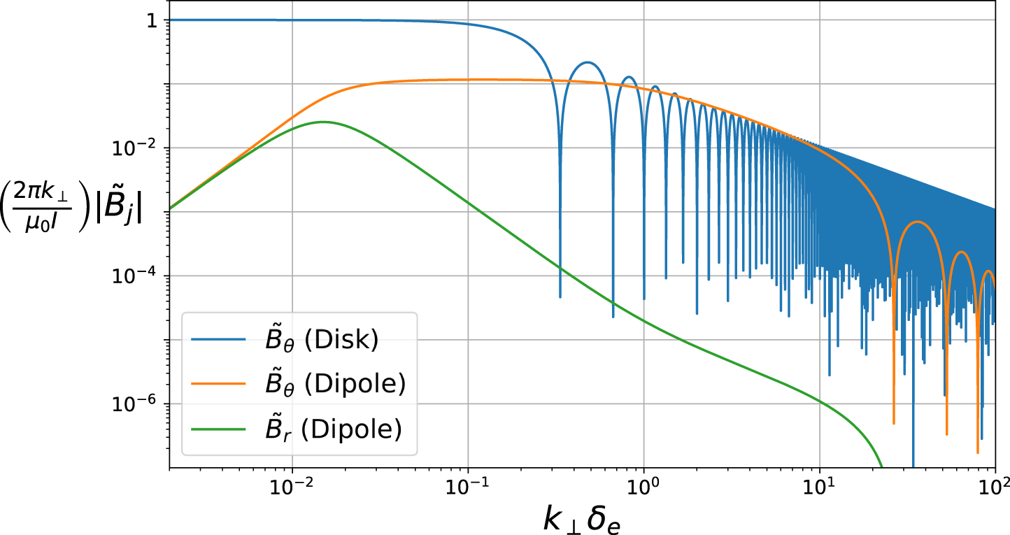
Figure 2. Magnitude of the magnetic field resulting from an electric dipole of length
 $\ell$
aligned along the background field, in a single-ion species plasma at frequency
$\ell$
aligned along the background field, in a single-ion species plasma at frequency
 $\unicode[STIX]{x1D714}=0.75\unicode[STIX]{x1D6FA}_{ci}$
. For comparison, we show the field resulting from a disk exciter with radius
$\unicode[STIX]{x1D714}=0.75\unicode[STIX]{x1D6FA}_{ci}$
. For comparison, we show the field resulting from a disk exciter with radius
 $\ell /2$
.
$\ell /2$
.

Figure 3. Comparison of the azimuthal field of the slow wave, fast wave and vacuum field, at a distance
 $z=v_{A}/\unicode[STIX]{x1D714}$
away from the electric dipole antenna. The same plasma and antenna conditions from figure 2 are assumed. The dashed line in the fast wave branch denotes where the wave is evanescent.
$z=v_{A}/\unicode[STIX]{x1D714}$
away from the electric dipole antenna. The same plasma and antenna conditions from figure 2 are assumed. The dashed line in the fast wave branch denotes where the wave is evanescent.
Equation (4.9) is commonly known as the inertial Alfvén wave. In the limit
 $k_{\bot }\rightarrow 0$
, the Alfvén wave is mediated entirely by the cross-field ion polarization and
$k_{\bot }\rightarrow 0$
, the Alfvén wave is mediated entirely by the cross-field ion polarization and
 $E\times B$
currents. When
$E\times B$
currents. When
 $k_{\bot }\neq 0$
, a parallel electron current is excited in order to satisfy current closure (i.e.
$k_{\bot }\neq 0$
, a parallel electron current is excited in order to satisfy current closure (i.e.
 $\unicode[STIX]{x1D735}\boldsymbol{\cdot }\boldsymbol{J}=0$
). When
$\unicode[STIX]{x1D735}\boldsymbol{\cdot }\boldsymbol{J}=0$
). When
 $n_{\bot }^{2}\gg |S|$
, the induced parallel electron current is so much larger than the cross-field currents that it becomes predominantly responsible for setting the perpendicular magnetic field of the wave – hence the dominant azimuthal magnetic field seen in the
$n_{\bot }^{2}\gg |S|$
, the induced parallel electron current is so much larger than the cross-field currents that it becomes predominantly responsible for setting the perpendicular magnetic field of the wave – hence the dominant azimuthal magnetic field seen in the
 $k_{\bot }\unicode[STIX]{x1D6FF}_{e}\gg 1$
regime. From inspection of (4.7) and (4.8), the coupled antenna power is zero when
$k_{\bot }\unicode[STIX]{x1D6FF}_{e}\gg 1$
regime. From inspection of (4.7) and (4.8), the coupled antenna power is zero when
 $\ell =n\unicode[STIX]{x1D706}_{\Vert }$
, for integer
$\ell =n\unicode[STIX]{x1D706}_{\Vert }$
, for integer
 $n$
, and greatest when
$n$
, and greatest when
 $\ell =({\textstyle \frac{1}{2}}+n)\unicode[STIX]{x1D706}_{\Vert }$
.
$\ell =({\textstyle \frac{1}{2}}+n)\unicode[STIX]{x1D706}_{\Vert }$
.
Previous analytic studies have been done on the spatial structure of Alfvén waves launched from a metal disk exciter, both in the inertial (Morales et al.
Reference Morales, Loritsch and Maggs1994) and kinetic (Morales & Maggs Reference Morales and Maggs1997) regimes. For a disk exciter of radius
 $a$
, maintained at a fixed AC voltage,
$a$
, maintained at a fixed AC voltage,
 $\tilde{B}_{\unicode[STIX]{x1D703}}(k_{\bot },z)$
was shown to have the following form:
$\tilde{B}_{\unicode[STIX]{x1D703}}(k_{\bot },z)$
was shown to have the following form:
 $$\begin{eqnarray}\tilde{B}_{\unicode[STIX]{x1D703}}(k_{\bot },z)={\displaystyle \frac{\unicode[STIX]{x1D707}_{0}I}{2\unicode[STIX]{x03C0}k_{\bot }}}{\displaystyle \frac{\sin k_{\bot }a}{k_{\bot }a}}.\end{eqnarray}$$
Figure 2 includes
 $\tilde{B}_{\unicode[STIX]{x1D703}}(k_{\bot },z)$
of a disk exciter antenna, with radius equal to half the dipole length, for comparison. The total integrated power of the disk exciter wave is much greater, which is due in part to the fact that the disk is in direct electrical contact with the plasma, whereas the dipole relies on capacitive coupling. In addition, the dipole experiences worse coupling at lower frequency, while the disk is unaffected.
$\tilde{B}_{\unicode[STIX]{x1D703}}(k_{\bot },z)$
of a disk exciter antenna, with radius equal to half the dipole length, for comparison. The total integrated power of the disk exciter wave is much greater, which is due in part to the fact that the disk is in direct electrical contact with the plasma, whereas the dipole relies on capacitive coupling. In addition, the dipole experiences worse coupling at lower frequency, while the disk is unaffected.
We previously asserted that the fast wave is evanescent for the plasma parameters being considered, as well as claiming that the vacuum field is much smaller than the radiative field far from the antenna. Figure 3 compares the magnitude of the slow wave to both the fast wave and vacuum field, at a distance
 $k_{A}z=1$
away from the dipole, where
$k_{A}z=1$
away from the dipole, where
 $k_{A}=\unicode[STIX]{x1D714}/v_{A}$
and
$k_{A}=\unicode[STIX]{x1D714}/v_{A}$
and
 $v_{A}$
is the Alfvén speed. The dashed line denotes evanescence. The fast wave is seen to be real and propagating at
$v_{A}$
is the Alfvén speed. The dashed line denotes evanescence. The fast wave is seen to be real and propagating at
 $k_{\bot }\unicode[STIX]{x1D6FF}_{e}\ll 1$
, but the vast majority of coupled power exists at values of
$k_{\bot }\unicode[STIX]{x1D6FF}_{e}\ll 1$
, but the vast majority of coupled power exists at values of
 $k_{\bot }$
where the fast wave is heavily evanescent. Additionally, the magnitude of the vacuum field is vanishingly small compared to that of the slow wave. We conclude that, given the assumed plasma conditions, the total magnetic field in the plasma far from the antenna (in the
$k_{\bot }$
where the fast wave is heavily evanescent. Additionally, the magnitude of the vacuum field is vanishingly small compared to that of the slow wave. We conclude that, given the assumed plasma conditions, the total magnetic field in the plasma far from the antenna (in the
 $\hat{z}$
direction) will be due entirely to propagating slow waves.
$\hat{z}$
direction) will be due entirely to propagating slow waves.
4.2 Near-field response
In the previous section we solved (3.6) for points far away from the antenna, which allowed us to drop the contribution due to backward propagating waves. We will now solve (3.6) everywhere in the plasma. In doing so, our goal is to see how near-field effects modify the resulting field for regions close to the antenna.
Ignoring the fast wave contribution as we did before, equation (3.6) can be written as the following:
 $$\begin{eqnarray}\tilde{B}_{\unicode[STIX]{x1D703}}(k_{\bot },z)=\tilde{B}_{\unicode[STIX]{x1D703}0}+{\displaystyle \frac{\text{i}(\unicode[STIX]{x1D714}^{4}/c^{4})}{2k_{\Vert }(k_{\Vert }^{2}-k_{\Vert -}^{2})}}\left[\int _{-\infty }^{z}\text{e}^{\text{i}k_{\Vert }(z-z^{\prime })}f(z^{\prime })\,\text{d}z^{\prime }+\int _{z}^{\infty }\text{e}^{-\text{i}k_{\Vert }(z-z^{\prime })}f(z^{\prime })\,\text{d}z^{\prime }\right].\end{eqnarray}$$
The interference between the forward and backward propagating waves, given by the first and second integrals respectively, is what will give rise to the near-field response. Note that we have included the vacuum field in the above solution. It was shown in the previous section that the vacuum field can be ignored far from the antenna, but we will show here that this is not the case in the near field.
The source term
 $f(z)$
can be found by inserting the (Hankel-transformed) vacuum field, given by (4.3), into (2.18)
$f(z)$
can be found by inserting the (Hankel-transformed) vacuum field, given by (4.3), into (2.18)
 $$\begin{eqnarray}f(z)={\displaystyle \frac{\unicode[STIX]{x1D707}_{0}I}{2\unicode[STIX]{x03C0}k_{\bot }}}\left\{\begin{array}{@{}ll@{}}-RL\text{e}^{-k_{\bot }z}\sinh k_{\bot }{\displaystyle \frac{\ell }{2}}\quad & \text{for }z>\ell /2,\\ Sn_{\bot }^{2}-RL(1-\text{e}^{-k_{\bot }(\ell /2)}\cosh k_{\bot }z)\quad & \text{for }-\ell /2<z<\ell /2,\\ -RL\text{e}^{k_{\bot }z}\sinh k_{\bot }{\displaystyle \frac{\ell }{2}}\quad & \text{for }z<-\ell /2.\end{array}\right.\end{eqnarray}$$
From here it is straightforward to insert the above expression for
 $f(z)$
into (4.11). Because our vacuum field is divided up into three distinct regions, equation (4.11) will have to be solved separately for the three different regions as well. For demonstrative purposes, we will consider the two outer regions first, defined by
$f(z)$
into (4.11). Because our vacuum field is divided up into three distinct regions, equation (4.11) will have to be solved separately for the three different regions as well. For demonstrative purposes, we will consider the two outer regions first, defined by
 $|z|>\ell /2$
. The solution to (4.11) for
$|z|>\ell /2$
. The solution to (4.11) for
 $z>\ell /2$
and
$z>\ell /2$
and
 $z<-\ell /2$
are given by the following:
$z<-\ell /2$
are given by the following:
 $$\begin{eqnarray}\displaystyle \tilde{B}_{\unicode[STIX]{x1D703}}(k_{\bot },z) & = & \displaystyle \underbrace{\text{i}{\displaystyle \frac{\unicode[STIX]{x1D707}_{0}I}{2\unicode[STIX]{x03C0}k_{\bot }}}\left(S-{\displaystyle \frac{RL}{n^{2}}}\right){\displaystyle \frac{n_{\bot }^{2}\text{e}^{\text{i}k_{\Vert }|z|}\sin k_{\Vert }{\displaystyle \frac{\ell }{2}}}{n_{\Vert }^{2}(n_{\Vert }^{2}-n_{\Vert -}^{2})}}}_{\mathit{Radiation\,\,field}}\nonumber\\ \displaystyle & & \displaystyle +\,\underbrace{{\displaystyle \frac{\unicode[STIX]{x1D707}_{0}I}{2\unicode[STIX]{x03C0}k_{\bot }}}\left(1+{\displaystyle \frac{RL}{n^{2}(n_{\Vert }^{2}-n_{\Vert -}^{2})}}\right)\text{e}^{-k_{\bot }|z|}\sinh k_{\bot }{\displaystyle \frac{\ell }{2}}}_{\mathit{Near}\text{-}\mathit{field\,\,response}}.\end{eqnarray}$$
The first term is identified as the radiation field, and is identical to the far-field response derived in the previous section, given by (4.7). The second term arises from the inclusion of the contribution from backward propagating waves in the general solution, and can be thought of as the near-field response. The near field in (4.13) is the sum of both the near-field plasma response as well as the vacuum field. The near field is observed to decay exponentially as one moves away from the antenna, dropping off much more rapidly for larger values of
 $k_{\bot }$
. Note that the near-field response does not propagate as a wave, like the radiation field, but rather is a region around the antenna which pulsates at frequency
$k_{\bot }$
. Note that the near-field response does not propagate as a wave, like the radiation field, but rather is a region around the antenna which pulsates at frequency
 $\unicode[STIX]{x1D714}$
.
$\unicode[STIX]{x1D714}$
.
The field in the region
 $-\ell /2<z<\ell /2$
is found from (4.11) to be the following:
$-\ell /2<z<\ell /2$
is found from (4.11) to be the following:
 $$\begin{eqnarray}\displaystyle \tilde{B}_{\unicode[STIX]{x1D703}}(k_{\bot },z) & = & \displaystyle {\displaystyle \frac{\unicode[STIX]{x1D707}_{0}I}{2\unicode[STIX]{x03C0}k_{\bot }}}{\displaystyle \frac{n_{\bot }^{2}}{n_{\Vert }^{2}(n_{\Vert }^{2}-n_{\Vert -}^{2})}}\left(S-{\displaystyle \frac{RL}{n^{2}}}\right)\left(\text{e}^{\text{i}k_{\Vert }(\ell /2)}\cos k_{\Vert }z-1\right)\nonumber\\ \displaystyle & & \displaystyle +\,{\displaystyle \frac{\unicode[STIX]{x1D707}_{0}I}{2\unicode[STIX]{x03C0}k_{\bot }}}\left(1+{\displaystyle \frac{RL}{n^{2}(n_{\Vert }^{2}-n_{\Vert -}^{2})}}\right)\left(1-\text{e}^{-k_{\bot }(\ell /2)}\cosh k_{\bot }z\right).\end{eqnarray}$$

Figure 4. Azimuthal magnetic field versus axial position
 $k_{A}z$
, due to an electric dipole antenna of length
$k_{A}z$
, due to an electric dipole antenna of length
 $\ell$
, for various values of
$\ell$
, for various values of
 $k_{\bot }$
. In the region
$k_{\bot }$
. In the region
 $|z|<\ell /2$
, near-field effects dominate. The near-field response decays exponentially with increasing
$|z|<\ell /2$
, near-field effects dominate. The near-field response decays exponentially with increasing
 $|z|$
, and far from the antenna only the radiation field remains.
$|z|$
, and far from the antenna only the radiation field remains.
Figure 4 shows how
 $\tilde{B}_{\unicode[STIX]{x1D703}}(k_{\bot },z)$
varies with
$\tilde{B}_{\unicode[STIX]{x1D703}}(k_{\bot },z)$
varies with
 $z$
, for several different values of
$z$
, for several different values of
 $k_{\bot }$
. The same plasma and antenna conditions as figures 2 and 3 were assumed. The field is peaked in the region
$k_{\bot }$
. The same plasma and antenna conditions as figures 2 and 3 were assumed. The field is peaked in the region
 $-\ell /2<z<\ell /2$
and drops off exponentially for
$-\ell /2<z<\ell /2$
and drops off exponentially for
 $|z|>\ell /2$
, with larger values of
$|z|>\ell /2$
, with larger values of
 $k_{\bot }$
experiencing a more abrupt drop off. The radiation zone for a given
$k_{\bot }$
experiencing a more abrupt drop off. The radiation zone for a given
 $k_{\bot }$
is defined as the region far enough from the antenna where the field exhibits wave-like motion, as the only remaining field out there is due to the propagating slow wave. In the limit
$k_{\bot }$
is defined as the region far enough from the antenna where the field exhibits wave-like motion, as the only remaining field out there is due to the propagating slow wave. In the limit
 $k_{\bot }\rightarrow \infty$
, the field in the vicinity of the antenna converges to a constant value of
$k_{\bot }\rightarrow \infty$
, the field in the vicinity of the antenna converges to a constant value of
 $\tilde{B}_{\unicode[STIX]{x1D703}}=\unicode[STIX]{x1D707}_{0}I/2\unicode[STIX]{x03C0}k_{\bot }$
, whereas the radiation field drops off more rapidly with increasing
$\tilde{B}_{\unicode[STIX]{x1D703}}=\unicode[STIX]{x1D707}_{0}I/2\unicode[STIX]{x03C0}k_{\bot }$
, whereas the radiation field drops off more rapidly with increasing
 $k_{\bot }$
.
$k_{\bot }$
.
4.3 Numerical results
The spatially resolved magnetic field is found from the inverse Hankel transform of
 $\tilde{B}_{\unicode[STIX]{x1D703}}(k_{\bot },z)$
. For the radiation field, this amounts to solving the following integral:
$\tilde{B}_{\unicode[STIX]{x1D703}}(k_{\bot },z)$
. For the radiation field, this amounts to solving the following integral:
 $$\begin{eqnarray}B_{\unicode[STIX]{x1D703}}(r,z,\unicode[STIX]{x1D714})=\text{i}{\displaystyle \frac{\unicode[STIX]{x1D707}_{0}I}{2\unicode[STIX]{x03C0}}}{\displaystyle \frac{\unicode[STIX]{x1D714}^{2}}{c^{2}}}\int _{0}^{\infty }\left(S-{\displaystyle \frac{\unicode[STIX]{x1D714}^{2}}{c^{2}}}{\displaystyle \frac{RL}{k^{2}}}\right){\displaystyle \frac{k_{\bot }^{2}\text{e}^{\text{i}k_{\Vert }z}\sin k_{\Vert }{\displaystyle \frac{\ell }{2}}}{k_{\Vert }^{2}(k_{\Vert }^{2}-k_{\Vert -}^{2})}}\text{J}_{1}(k_{\bot }r)\,\text{d}k_{\bot },\end{eqnarray}$$
where
 $k_{\Vert }$
and
$k_{\Vert }$
and
 $k_{\Vert -}$
are the slow and fast wave dispersions, respectively, and are given by (2.17). Equation (4.15) will, in general, need to be solved numerically. The time-resolved field is then found from the real part of
$k_{\Vert -}$
are the slow and fast wave dispersions, respectively, and are given by (2.17). Equation (4.15) will, in general, need to be solved numerically. The time-resolved field is then found from the real part of
 $B_{\unicode[STIX]{x1D703}}(r,z,\unicode[STIX]{x1D714})\text{e}^{-\text{i}\unicode[STIX]{x1D714}t}$
. Close to the antenna, the near-field solution given by (4.13) and (4.14) should be used. The results that follow in this section assume the same plasma conditions as before. Numerical integration of (4.15) was done using the algorithm devised by Ogata (Reference Ogata2005), which uses a quadrature formula with the zeros of the Bessel function as nodes.
$B_{\unicode[STIX]{x1D703}}(r,z,\unicode[STIX]{x1D714})\text{e}^{-\text{i}\unicode[STIX]{x1D714}t}$
. Close to the antenna, the near-field solution given by (4.13) and (4.14) should be used. The results that follow in this section assume the same plasma conditions as before. Numerical integration of (4.15) was done using the algorithm devised by Ogata (Reference Ogata2005), which uses a quadrature formula with the zeros of the Bessel function as nodes.

Figure 5. Time animation of the azimuthal magnetic field of the slow wave launched from an electric dipole, for frequencies (a)
 $0.25\unicode[STIX]{x1D6FA}_{ci}$
and (b)
$0.25\unicode[STIX]{x1D6FA}_{ci}$
and (b)
 $0.75\unicode[STIX]{x1D6FA}_{ci}$
. The
$0.75\unicode[STIX]{x1D6FA}_{ci}$
. The
 $z$
axis was normalized to the antenna length
$z$
axis was normalized to the antenna length
 $\ell$
to show how the parallel wavelength decreases with increasing frequency. The propagation angle of the cones emanating from either end of the dipole can be determined from the inertial Alfvén wave dispersion.
$\ell$
to show how the parallel wavelength decreases with increasing frequency. The propagation angle of the cones emanating from either end of the dipole can be determined from the inertial Alfvén wave dispersion.
Figure 5 shows the time evolution of the resulting waveform, for two different frequencies. Two conical structures are seen emanating from either end of the dipole, with an angle of propagation that increases with frequency. The cone’s propagation angle can be found from the ratio of the wave’s perpendicular and parallel group velocities. For antennae whose scale length is of the order of the electron skin depth
 $\unicode[STIX]{x1D6FF}_{e}\equiv c/\unicode[STIX]{x1D714}_{pe}$
, the majority of antenna power couples to large enough values of
$\unicode[STIX]{x1D6FF}_{e}\equiv c/\unicode[STIX]{x1D714}_{pe}$
, the majority of antenna power couples to large enough values of
 $k_{\bot }$
where the inertial Alfvén wave dispersion, given by (4.9), is valid. The ratio of the inertial wave’s perpendicular to parallel group velocities gives the propagation angle of the wave
$k_{\bot }$
where the inertial Alfvén wave dispersion, given by (4.9), is valid. The ratio of the inertial wave’s perpendicular to parallel group velocities gives the propagation angle of the wave
 $$\begin{eqnarray}\tan \unicode[STIX]{x1D703}=\left|{\displaystyle \frac{\unicode[STIX]{x2202}\unicode[STIX]{x1D714}/\unicode[STIX]{x2202}k_{\bot }}{\unicode[STIX]{x2202}\unicode[STIX]{x1D714}/\unicode[STIX]{x2202}k_{\Vert }}}\right|=\sqrt{{\displaystyle \frac{m_{e}}{m_{i}}}}{\displaystyle \frac{\unicode[STIX]{x1D714}}{\sqrt{\unicode[STIX]{x1D6FA}_{ci}^{2}-\unicode[STIX]{x1D714}^{2}}}}{\displaystyle \frac{k_{\bot }\unicode[STIX]{x1D6FF}_{e}}{\sqrt{1+k_{\bot }^{2}\unicode[STIX]{x1D6FF}_{e}^{2}}}},\end{eqnarray}$$
when
 $k_{\bot }\unicode[STIX]{x1D6FF}_{e}\gg 1$
, the propagation angle approaches an asymptotic limit that is independent of
$k_{\bot }\unicode[STIX]{x1D6FF}_{e}\gg 1$
, the propagation angle approaches an asymptotic limit that is independent of
 $k_{\bot }$
, resulting in a conical structure. The propagation angle
$k_{\bot }$
, resulting in a conical structure. The propagation angle
 $\unicode[STIX]{x1D703}_{c}$
of the cone is given by
$\unicode[STIX]{x1D703}_{c}$
of the cone is given by
 $$\begin{eqnarray}\tan \unicode[STIX]{x1D703}_{c}=\sqrt{{\displaystyle \frac{m_{e}}{m_{i}}}}{\displaystyle \frac{\bar{\unicode[STIX]{x1D714}}}{\sqrt{1-\bar{\unicode[STIX]{x1D714}}^{2}}}},\end{eqnarray}$$
where
 $\bar{\unicode[STIX]{x1D714}}=\unicode[STIX]{x1D714}/\unicode[STIX]{x1D6FA}_{ci}$
. The propagation angles observed in figure 5 are in close agreement with (4.17). Similar conical spreading was predicted to exist for Alfvén waves launched by a metal disk exciter in a cold plasma (Morales et al.
Reference Morales, Loritsch and Maggs1994), and was consequently observed in the laboratory (Gekelman et al.
Reference Gekelman, Vincena, Leneman and Maggs1994). The amplitude of the field is shown in figure 6 at various axial positions. At each
$\bar{\unicode[STIX]{x1D714}}=\unicode[STIX]{x1D714}/\unicode[STIX]{x1D6FA}_{ci}$
. The propagation angles observed in figure 5 are in close agreement with (4.17). Similar conical spreading was predicted to exist for Alfvén waves launched by a metal disk exciter in a cold plasma (Morales et al.
Reference Morales, Loritsch and Maggs1994), and was consequently observed in the laboratory (Gekelman et al.
Reference Gekelman, Vincena, Leneman and Maggs1994). The amplitude of the field is shown in figure 6 at various axial positions. At each
 $z$
position, the field is observed to increase with increasing
$z$
position, the field is observed to increase with increasing
 $r$
until it reaches the edge of the cone, where it exhibits a
$r$
until it reaches the edge of the cone, where it exhibits a
 $1/r$
drop-off. The
$1/r$
drop-off. The
 $1/r$
dependence outside the cone suggests that the parallel plasma current excited by the antenna is contained entirely within the conical region. Additionally, the magnitude of the field outside the cone is constant with
$1/r$
dependence outside the cone suggests that the parallel plasma current excited by the antenna is contained entirely within the conical region. Additionally, the magnitude of the field outside the cone is constant with
 $z$
in the radiation zone of the plasma, as the total parallel plasma current is conserved with
$z$
in the radiation zone of the plasma, as the total parallel plasma current is conserved with
 $z$
. The inclusion of electron collisionality, which we have omitted for demonstrative purposes, results in a field outside the cone which decays with
$z$
. The inclusion of electron collisionality, which we have omitted for demonstrative purposes, results in a field outside the cone which decays with
 $z$
. Far from the antenna, where
$z$
. Far from the antenna, where
 $k_{A}z\gg 1$
, diffraction patterns begin to emerge in the radial profile. All these results are consistent with countless previous experimental studies of inertial Alfvén waves in the LAPD (Gekelman et al.
Reference Gekelman, Vincena, Compernolle, Morales, Maggs, Pribyl and Carter2011). For a disk exciter antenna whose radius is of the order of the electron skin depth, the wave’s radial profile experiences a strong azimuthal magnetic field with an off-axis maximum that spreads out conically with increasing
$k_{A}z\gg 1$
, diffraction patterns begin to emerge in the radial profile. All these results are consistent with countless previous experimental studies of inertial Alfvén waves in the LAPD (Gekelman et al.
Reference Gekelman, Vincena, Compernolle, Morales, Maggs, Pribyl and Carter2011). For a disk exciter antenna whose radius is of the order of the electron skin depth, the wave’s radial profile experiences a strong azimuthal magnetic field with an off-axis maximum that spreads out conically with increasing
 $z$
, eventually producing a radial diffraction pattern far from the disk.
$z$
, eventually producing a radial diffraction pattern far from the disk.

Figure 6. Amplitude of the azimuthal magnetic field versus radius, at various distances from the antenna. The field increases with radius up until a certain point, where it exhibits a
 $1/r$
drop off.
$1/r$
drop off.
4.4 Fast wave considerations
In the previous section we asserted that the fast wave was evanescent for the assumed plasma conditions, and therefore focused exclusively on the spatial structure of the slow wave. While it is straightforward to prove the fast wave’s contribution is negligible in the far field, the same is not obvious in the vicinity of the antenna. For the relatively large values of
 $k_{\bot }$
imposed by our assumed antenna, it can be shown that the fast wave dispersion, given by the
$k_{\bot }$
imposed by our assumed antenna, it can be shown that the fast wave dispersion, given by the
 $\pm \rightarrow -$
branch of (2.17), can be approximated by the following:
$\pm \rightarrow -$
branch of (2.17), can be approximated by the following:
 $$\begin{eqnarray}n_{\Vert }^{2}=S-n_{\bot }^{2}.\end{eqnarray}$$
Since
 $n_{\bot }^{2}\gg |S|$
, equation (4.18) suggests the fast wave will be purely evanescent. We can find the fast wave’s magnetic field from (4.13) and (4.14), but with the fast and slow wave dispersions switched. Substituting the above dispersion into these two equations, we get the following approximate form of the field for the fast wave:
$n_{\bot }^{2}\gg |S|$
, equation (4.18) suggests the fast wave will be purely evanescent. We can find the fast wave’s magnetic field from (4.13) and (4.14), but with the fast and slow wave dispersions switched. Substituting the above dispersion into these two equations, we get the following approximate form of the field for the fast wave:
 $$\begin{eqnarray}\tilde{B}_{\unicode[STIX]{x1D703}}(k_{\bot },z)=-{\displaystyle \frac{\unicode[STIX]{x1D707}_{0}I}{2\unicode[STIX]{x03C0}k_{\bot }}}{\displaystyle \frac{S}{n_{\bot }^{2}}}\left\{\begin{array}{@{}ll@{}}\text{e}^{-k_{\bot }|z|}\sinh k_{\bot }{\displaystyle \frac{\ell }{2}}\quad & \text{for }|z|>\ell /2,\\ 1-\text{e}^{-k_{\bot }(\ell /2)}\cosh k_{\bot }z\quad & \text{for }|z|<\ell /2.\end{array}\right.\end{eqnarray}$$
Note that (4.19) ignores the small part of the
 $k_{\bot }$
spectrum which contributes propagating waves, as can be seen in figure 3. Comparing the above equation to the vacuum field, given by (4.2), we see that the fast wave is a factor of
$k_{\bot }$
spectrum which contributes propagating waves, as can be seen in figure 3. Comparing the above equation to the vacuum field, given by (4.2), we see that the fast wave is a factor of
 $S/n_{\bot }^{2}$
smaller than the vacuum field’s contribution. In the region
$S/n_{\bot }^{2}$
smaller than the vacuum field’s contribution. In the region
 $|z|>\ell /2$
, it is straightforward to show that the exponentially decaying near field is dominated by the vacuum field, followed by the evanescent fast wave and then the near-field part of the slow wave. Similarly, in the region
$|z|>\ell /2$
, it is straightforward to show that the exponentially decaying near field is dominated by the vacuum field, followed by the evanescent fast wave and then the near-field part of the slow wave. Similarly, in the region
 $|z|<\ell /2$
, the near field is again dominated by the vacuum field, followed by the slow wave and then the fast wave.
$|z|<\ell /2$
, the near field is again dominated by the vacuum field, followed by the slow wave and then the fast wave.
In plasmas with sufficiently high density to permit fast wave propagation, or alternatively at high enough frequencies where
 $n_{\bot }^{2}\gg |S|$
is no longer satisfied, the physics of the near field is expected to change drastically and may be dominated by the slow wave, fast wave or both. Looking at the slow wave solution given by (4.13), the slow wave’s near-field plasma response will be larger than the vacuum field when the following condition is satisfied:
$n_{\bot }^{2}\gg |S|$
is no longer satisfied, the physics of the near field is expected to change drastically and may be dominated by the slow wave, fast wave or both. Looking at the slow wave solution given by (4.13), the slow wave’s near-field plasma response will be larger than the vacuum field when the following condition is satisfied:
 $$\begin{eqnarray}\left|{\displaystyle \frac{RL}{n^{2}(n_{\Vert }^{2}-n_{\Vert -}^{2})}}\right|>1.\end{eqnarray}$$
Since the approximate form of the fast wave solution, given by (4.19), is predicated on the assumption
 $n_{\bot }^{2}\gg |S|$
, a deeper investigation of the fast wave is warranted in order to determine the conditions for fast wave dominance in the near field.
$n_{\bot }^{2}\gg |S|$
, a deeper investigation of the fast wave is warranted in order to determine the conditions for fast wave dominance in the near field.
5 Generalized solution to the antenna wave equation in Cartesian coordinates
In the preceding sections we found the solution to the antenna equation for an azimuthally symmetric antenna. While this solution was instructive in highlighting the underlying physics, it is useless for antennae which do not possess azimuthal symmetry. In this section we will derive the fully generalized solution to the antenna wave equation in Cartesian coordinates. We will again assume a cold, magnetized plasma and frequencies such that the vacuum displacement current can be ignored, but aside from that we will abstain from making any limiting assumptions about our system. Our starting point is (2.3), which can be separated into the following system of equations:
 $$\begin{eqnarray}\displaystyle & \displaystyle \text{i}n_{y}\left(\text{i}n_{x}\tilde{E_{y}}-\text{i}n_{y}\tilde{E}_{x}\right)-{\displaystyle \frac{\unicode[STIX]{x2202}}{\unicode[STIX]{x2202}\bar{z}}}\left({\displaystyle \frac{\unicode[STIX]{x2202}\tilde{E}_{x}}{\unicode[STIX]{x2202}\bar{z}}}-\text{i}n_{x}\tilde{E}_{z}\right)-S\tilde{E}_{x}+\text{i}D\tilde{E}_{y}=S\tilde{E}_{x0}-\text{i}D\tilde{E}_{y0}, & \displaystyle\end{eqnarray}$$
 $$\begin{eqnarray}\displaystyle & \displaystyle {\displaystyle \frac{\unicode[STIX]{x2202}}{\unicode[STIX]{x2202}\bar{z}}}\left(\text{i}n_{y}\tilde{E}_{z}-{\displaystyle \frac{\unicode[STIX]{x2202}\tilde{E}_{y}}{\unicode[STIX]{x2202}\bar{z}}}\right)-\text{i}n_{x}\left(\text{i}n_{x}\tilde{E}_{y}-\text{i}n_{y}\tilde{E}_{x}\right)-\text{i}D\tilde{E}_{x}-S\tilde{E}_{y}=\text{i}D\tilde{E}_{x0}+S\tilde{E}_{y0}, & \displaystyle\end{eqnarray}$$
 $$\begin{eqnarray}\displaystyle & \displaystyle \text{i}n_{x}\left({\displaystyle \frac{\unicode[STIX]{x2202}\tilde{E}_{x}}{\unicode[STIX]{x2202}\bar{z}}}-\text{i}n_{x}\tilde{E}_{z}\right)-\text{i}n_{y}\left(\text{i}n_{y}\tilde{E}_{z}-{\displaystyle \frac{\unicode[STIX]{x2202}\tilde{E}_{y}}{\unicode[STIX]{x2202}\bar{z}}}\right)-P\tilde{E}_{z}=P\tilde{E}_{z0}, & \displaystyle\end{eqnarray}$$
where we dropped the vacuum displacement current, and have defined
 $\bar{z}\equiv (c/\unicode[STIX]{x1D714})z$
.
$\bar{z}\equiv (c/\unicode[STIX]{x1D714})z$
.
 $\tilde{E}_{j}(k_{x},k_{y},z)$
is the Fourier transform of
$\tilde{E}_{j}(k_{x},k_{y},z)$
is the Fourier transform of
 $E_{j}(x,y,z)$
in the
$E_{j}(x,y,z)$
in the
 $x$
and
$x$
and
 $y$
directions, given by
$y$
directions, given by
 $$\begin{eqnarray}\tilde{E}_{j}(k_{x},k_{y},z)=\int _{-\infty }^{\infty }\int _{-\infty }^{\infty }E_{j}(x,y,z)\text{e}^{-\text{i}k_{x}x}\text{e}^{-\text{i}k_{y}y}\,\text{d}x\,\text{d}y.\end{eqnarray}$$
Equations (5.1)–(5.3) can be expressed in terms of the magnetic field
 $\boldsymbol{B}$
via the following transformations:
$\boldsymbol{B}$
via the following transformations:
 $$\begin{eqnarray}\left.\begin{array}{@{}c@{}}\displaystyle (\text{i}n_{y}S-n_{x}D)[\text{(}\text{5.1}\text{)}\text{}]-(\text{i}n_{x}S+n_{y}D)[\text{(}\text{5.2}\text{)}\text{}],\\ \displaystyle P{\displaystyle \frac{\unicode[STIX]{x2202}}{\unicode[STIX]{x2202}\bar{z}}}[\text{(}\text{5.1}\text{)}\text{}]-(\text{i}n_{x}S+n_{y}D)[\text{(}\text{5.3}\text{)}\text{}],\\ \displaystyle P{\displaystyle \frac{\unicode[STIX]{x2202}}{\unicode[STIX]{x2202}\bar{z}}}[\text{(}\text{5.2}\text{)}\text{}]-(\text{i}n_{y}S-n_{x}D)[\text{(}\text{5.3}\text{)}\text{}].\end{array}\right\}\end{eqnarray}$$
The resulting three equations are as follows:
 $$\begin{eqnarray}(\text{i}n_{x}S+n_{y}D){\displaystyle \frac{\unicode[STIX]{x2202}\tilde{B}_{x}}{\unicode[STIX]{x2202}\bar{z}}}+(\text{i}n_{y}S-n_{x}D){\displaystyle \frac{\unicode[STIX]{x2202}\tilde{B}_{y}}{\unicode[STIX]{x2202}\bar{z}}}-(RL-Sn_{\bot }^{2})\tilde{B}_{z}=RL\tilde{B}_{z0},\end{eqnarray}$$
 $$\begin{eqnarray}\displaystyle & & \displaystyle (-\text{i}n_{y}^{2}D+n_{x}n_{y}S+\text{i}DP)\tilde{B}_{x}+(-n_{x}^{2}S+\text{i}n_{x}n_{y}D+SP)\tilde{B}_{y}\nonumber\\ \displaystyle & & \displaystyle \quad -\,\text{i}n_{y}P{\displaystyle \frac{\unicode[STIX]{x2202}\tilde{B}_{z}}{\unicode[STIX]{x2202}\bar{z}}}+P{\displaystyle \frac{\unicode[STIX]{x2202}^{2}\tilde{B}_{y}}{\unicode[STIX]{x2202}\bar{z}^{2}}}=-\text{i}DP\tilde{B}_{x0}-SP\tilde{B}_{y0},\end{eqnarray}$$
 $$\begin{eqnarray}\displaystyle & & \displaystyle (-n_{y}^{2}S-\text{i}n_{x}n_{y}D+SP)\tilde{B}_{x}+(\text{i}n_{x}^{2}D+n_{x}n_{y}S-\text{i}DP)\tilde{B}_{y}\nonumber\\ \displaystyle & & \displaystyle \quad -\,\text{i}n_{x}P{\displaystyle \frac{\unicode[STIX]{x2202}\tilde{B}_{z}}{\unicode[STIX]{x2202}\bar{z}}}+P{\displaystyle \frac{\unicode[STIX]{x2202}^{2}\tilde{B}_{x}}{\unicode[STIX]{x2202}\bar{z}^{2}}}=-SP\tilde{B}_{x0}+\text{i}DP\tilde{B}_{y0}.\end{eqnarray}$$
Equation (5.6) can be inserted into (5.7) and (5.8) to eliminate
 $\tilde{B}_{z}$
, resulting in two coupled differential equations for
$\tilde{B}_{z}$
, resulting in two coupled differential equations for
 $\tilde{B}_{x}$
and
$\tilde{B}_{x}$
and
 $\tilde{B}_{y}$
 $$\begin{eqnarray}\displaystyle & & \displaystyle \left[{\displaystyle \frac{\text{i}n_{y}P(\text{i}n_{x}S+n_{y}D)}{RL-Sn_{\bot }^{2}}}\right]{\displaystyle \frac{\unicode[STIX]{x2202}^{2}\tilde{B}_{x}}{\unicode[STIX]{x2202}\bar{z}^{2}}}+\left[{\displaystyle \frac{\text{i}n_{y}P(\text{i}n_{y}S-n_{x}D)}{RL-Sn_{\bot }^{2}}}-P\right]{\displaystyle \frac{\unicode[STIX]{x2202}^{2}\tilde{B}_{y}}{\unicode[STIX]{x2202}\bar{z}^{2}}}\nonumber\\ \displaystyle & & \displaystyle \qquad +\,\left[\text{i}n_{y}(\text{i}n_{x}S+n_{y}D)-\text{i}DP\right]\tilde{B}_{x}+\left[-\text{i}n_{x}(\text{i}n_{x}S+n_{y}D)-SP\right]\tilde{B}_{y}\nonumber\\ \displaystyle & & \displaystyle \quad =\left[{\displaystyle \frac{\text{i}n_{y}PRL}{RL-Sn_{\bot }^{2}}}\right]{\displaystyle \frac{\unicode[STIX]{x2202}\tilde{B}_{z0}}{\unicode[STIX]{x2202}\bar{z}}}+\text{i}DP\tilde{B}_{x0}+SP\tilde{B}_{y0},\end{eqnarray}$$
 $$\begin{eqnarray}\displaystyle & & \displaystyle \left[{\displaystyle \frac{-\text{i}n_{x}P(\text{i}n_{x}S+n_{y}D)}{RL-Sn_{\bot }^{2}}}+P\right]{\displaystyle \frac{\unicode[STIX]{x2202}^{2}\tilde{B}_{x}}{\unicode[STIX]{x2202}\bar{z}^{2}}}+\left[{\displaystyle \frac{-\text{i}n_{x}P(\text{i}n_{y}S-n_{x}D)}{RL-Sn_{\bot }^{2}}}\right]{\displaystyle \frac{\unicode[STIX]{x2202}^{2}\tilde{B}_{y}}{\unicode[STIX]{x2202}\bar{z}^{2}}}\nonumber\\ \displaystyle & & \displaystyle \qquad +\,\left[\text{i}n_{y}(\text{i}n_{y}S-n_{x}D)+SP\right]\tilde{B}_{x}+\left[-\text{i}n_{x}(\text{i}n_{y}S-n_{x}D)-\text{i}DP\right]\tilde{B}_{y}\nonumber\\ \displaystyle & & \displaystyle \quad =\left[{\displaystyle \frac{-\text{i}n_{x}PRL}{RL-Sn_{\bot }^{2}}}\right]{\displaystyle \frac{\unicode[STIX]{x2202}\tilde{B}_{z0}}{\unicode[STIX]{x2202}\bar{z}}}-SP\tilde{B}_{x0}+\text{i}DP\tilde{B}_{y0}.\end{eqnarray}$$
Equations (5.9) and (5.10) can be decoupled to get a differential equation for either
 $\tilde{B}_{x}$
or
$\tilde{B}_{x}$
or
 $\tilde{B}_{y}$
, although the math is rather tedious. The final result is two fourth-order differential equations for
$\tilde{B}_{y}$
, although the math is rather tedious. The final result is two fourth-order differential equations for
 $\tilde{B}_{x}$
and
$\tilde{B}_{x}$
and
 $\tilde{B}_{y}$
, given by
$\tilde{B}_{y}$
, given by
 $$\begin{eqnarray}\left({\displaystyle \frac{\unicode[STIX]{x2202}^{2}}{\unicode[STIX]{x2202}z^{2}}}+k_{\Vert +}^{2}\right)\left({\displaystyle \frac{\unicode[STIX]{x2202}^{2}}{\unicode[STIX]{x2202}z^{2}}}+k_{\Vert -}^{2}\right)\left[\begin{array}{@{}c@{}}\tilde{B}_{x}\\ \tilde{B}_{y}\end{array}\right]={\displaystyle \frac{\unicode[STIX]{x1D714}^{4}}{c^{4}}}\left[\begin{array}{@{}c@{}}f(z)\\ g(z)\end{array}\right],\end{eqnarray}$$
where
 $k_{\Vert \pm }$
is given by the following dispersion relation:
$k_{\Vert \pm }$
is given by the following dispersion relation:
 $$\begin{eqnarray}\left({\displaystyle \frac{c^{2}}{\unicode[STIX]{x1D714}^{2}}}\right)k_{\Vert \pm }^{2}=S-{\displaystyle \frac{n_{\bot }^{2}}{2}}\left(1+{\displaystyle \frac{S}{P}}\right)\pm \sqrt{\left({\displaystyle \frac{n_{\bot }^{2}}{2}}\right)^{2}\left(1-{\displaystyle \frac{S}{P}}\right)^{2}+D^{2}\left(1-{\displaystyle \frac{n_{\bot }^{2}}{P}}\right)},\end{eqnarray}$$
where
 $n_{\bot }^{2}=n_{x}^{2}+n_{y}^{2}$
. Aside from the new definition of
$n_{\bot }^{2}=n_{x}^{2}+n_{y}^{2}$
. Aside from the new definition of
 $n_{\bot }^{2}$
, this dispersion relation is identical to the one derived in cylindrical coordinates in (2.17). The source terms
$n_{\bot }^{2}$
, this dispersion relation is identical to the one derived in cylindrical coordinates in (2.17). The source terms
 $f(z)$
and
$f(z)$
and
 $g(z)$
are given by the following:
$g(z)$
are given by the following:
 $$\begin{eqnarray}\displaystyle f(z) & = & \displaystyle -S{\displaystyle \frac{\unicode[STIX]{x2202}^{2}\tilde{B}_{x0}}{\unicode[STIX]{x2202}\bar{z}^{2}}}+\text{i}D{\displaystyle \frac{\unicode[STIX]{x2202}^{2}\tilde{B}_{y0}}{\unicode[STIX]{x2202}\bar{z}^{2}}}+\left[-\text{i}n_{y}(\text{i}n_{y}S+n_{x}D)-RL\left(1-{\displaystyle \frac{n_{x}^{2}}{P}}\right)\right]\tilde{B}_{x0}\nonumber\\ \displaystyle & & \displaystyle +\,\left[\text{i}n_{y}(\text{i}n_{x}S-n_{y}D)+n_{x}n_{y}{\displaystyle \frac{RL}{P}}\right]\tilde{B}_{y0},\end{eqnarray}$$
 $$\begin{eqnarray}\displaystyle g(z) & = & \displaystyle -\text{i}D{\displaystyle \frac{\unicode[STIX]{x2202}^{2}\tilde{B}_{x0}}{\unicode[STIX]{x2202}\bar{z}^{2}}}-S{\displaystyle \frac{\unicode[STIX]{x2202}^{2}\tilde{B}_{y0}}{\unicode[STIX]{x2202}\bar{z}^{2}}}+\left[\text{i}n_{x}(\text{i}n_{y}S+n_{x}D)+n_{x}n_{y}{\displaystyle \frac{RL}{P}}\right]\tilde{B}_{x0}\nonumber\\ \displaystyle & & \displaystyle +\,\left[-\text{i}n_{x}(\text{i}n_{x}S-n_{y}D)-RL\left(1-{\displaystyle \frac{n_{y}^{2}}{P}}\right)\right]\tilde{B}_{y0}.\end{eqnarray}$$
Alternatively, one can combine (5.7) and (5.8) with
 $\unicode[STIX]{x1D735}\boldsymbol{\cdot }\boldsymbol{B}=0$
, and they will arrive at the same fourth-order differential equation given by (5.11). Equation (5.11) is identical to the differential equation that was solved in § 3 for cylindrical coordinates, and so its general solution is the same
$\unicode[STIX]{x1D735}\boldsymbol{\cdot }\boldsymbol{B}=0$
, and they will arrive at the same fourth-order differential equation given by (5.11). Equation (5.11) is identical to the differential equation that was solved in § 3 for cylindrical coordinates, and so its general solution is the same
 $$\begin{eqnarray}\displaystyle \hspace{-24.0pt}\left[\begin{array}{@{}c@{}}\tilde{B}_{x}(k_{x},k_{y},z)\\ \tilde{B}_{y}(k_{x},k_{y},z)\end{array}\right] & = & \displaystyle {\displaystyle \frac{\unicode[STIX]{x1D714}^{4}}{c^{4}}}\int _{-\infty }^{z}\left[{\displaystyle \frac{\text{i}\text{e}^{\text{i}k_{\Vert +}\left(z-z^{\prime }\right)}}{2k_{\Vert +}(k_{\Vert +}^{2}-k_{\Vert -}^{2})}}+{\displaystyle \frac{\text{i}\text{e}^{\text{i}k_{\Vert -}(z-z^{\prime })}}{2k_{\Vert -}(k_{\Vert -}^{2}-k_{\Vert +}^{2})}}\right]\left[\begin{array}{@{}c@{}}f(z^{\prime })\\ g(z^{\prime })\end{array}\right]\text{d}z^{\prime }\nonumber\\ \displaystyle \hspace{-24.0pt} & & \displaystyle +\,{\displaystyle \frac{\unicode[STIX]{x1D714}^{4}}{c^{4}}}\int _{z}^{\infty }\left[{\displaystyle \frac{\text{i}\text{e}^{-\text{i}k_{\Vert +}\left(z-z^{\prime }\right)}}{2k_{\Vert +}(k_{\Vert +}^{2}-k_{\Vert -}^{2})}}+{\displaystyle \frac{\text{i}\text{e}^{-\text{i}k_{\Vert -}(z-z^{\prime })}}{2k_{\Vert -}(k_{\Vert -}^{2}-k_{\Vert +}^{2})}}\right]\left[\begin{array}{@{}c@{}}f(z^{\prime })\\ g(z^{\prime })\end{array}\right]\text{d}z^{\prime }.\end{eqnarray}$$
The Cartesian source terms given by (5.13) and (5.14) are lengthier than their azimuthally symmetric counterparts (equations (2.18) and (2.20)), but that is the trade-off we make in developing a fully generalized Cartesian solution. When
 $n_{y}=0$
, the variable substitutions
$n_{y}=0$
, the variable substitutions
 $x\rightarrow r$
and
$x\rightarrow r$
and
 $y\rightarrow \unicode[STIX]{x1D703}$
in (5.12)–(5.15) will return the general solution that was derived for the azimuthally symmetric case in § 3. A fully generalized solution to the homogeneous cold plasma wave equation in cylindrical coordinates is given by Ram & Hizanidis (Reference Ram and Hizanidis2016), and consists of an infinite summation of Bessel function eigenmodes. Depending on the geometry of a given antenna, it may be advantageous to use either the generalized Cartesian solution above or the generalized cylindrical solution.
$y\rightarrow \unicode[STIX]{x1D703}$
in (5.12)–(5.15) will return the general solution that was derived for the azimuthally symmetric case in § 3. A fully generalized solution to the homogeneous cold plasma wave equation in cylindrical coordinates is given by Ram & Hizanidis (Reference Ram and Hizanidis2016), and consists of an infinite summation of Bessel function eigenmodes. Depending on the geometry of a given antenna, it may be advantageous to use either the generalized Cartesian solution above or the generalized cylindrical solution.
6 Discussion and concluding remarks
In this paper we successfully developed a semi-analytic model for determining the electromagnetic field due to a current-driven antenna in a cold, magnetized plasma. We showed in § 2 that the vacuum electric field of the antenna couples to the plasma conductivity tensor and acts as a source that drives plasma waves. In § 3, we derived a general solution to the antenna wave equation for antennae with azimuthal symmetry. The general solution is a superposition of the fast and slow waves, which are the two fundamental modes of the cold plasma. It is typical in many laboratory plasmas for the fast wave to be evanescent, with only the slow wave being measurable far away from the antenna. In spite of this, it was shown that the fast wave physics cannot be ignored due to the fact that the antenna will always couple to both branches, even if one of them is evanescent. This is reflected in the general solution of (3.6), which shows that the amplitude of the slow wave is a function of the fast wave dispersion (and vice versa).
At every point in the plasma, the vacuum field of the antenna acts as an infinitesimal point source emitter that launches both forward and backward propagating waves. The total field is then found from the aggregate sum of all these infinitesimal point sources, which is the physical interpretation of the integral across the vacuum field in (3.6). For observation points close to the antenna, the interference of forward and backward propagating waves gives rise to what we refer to as the ‘near field’ of the antenna. Far away from the antenna, the field is shown to be a superposition of propagating plane waves (forward propagating for
 $z\gg 0$
, and backwards for
$z\gg 0$
, and backwards for
 $z\ll 0$
). Because of this, we define the radiation zone of the plasma as the region sufficiently far away from the antenna such that the near field and vacuum field are vanishingly small compared to the propagating part of the field. In deriving (3.6), we made the assumption that our plasma is infinite and unbounded, which allowed us to ignore possible complications due to reflected waves. Section 3 can be generalized to allow solutions which account for finite plasma boundaries, although this adds an additional layer of complexity that is outside the scope of the present discussion.
$z\ll 0$
). Because of this, we define the radiation zone of the plasma as the region sufficiently far away from the antenna such that the near field and vacuum field are vanishingly small compared to the propagating part of the field. In deriving (3.6), we made the assumption that our plasma is infinite and unbounded, which allowed us to ignore possible complications due to reflected waves. Section 3 can be generalized to allow solutions which account for finite plasma boundaries, although this adds an additional layer of complexity that is outside the scope of the present discussion.
In order to show how this model can be applied, we solved it for the case of an electric dipole antenna aligned along the background magnetic field. For plasma conditions that are typical of laboratory plasmas, such as those found in the LAPD, we showed that the magnetic field is almost entirely azimuthal with the majority of its power at large values of
 $k_{\bot }$
, where the slow wave is commonly known as the inertial Alfvén wave. The wave was shown to emit cones out of either end of the dipole, where the angle of propagation is given by (4.17). This is consistent with previous analytic studies of inertial Alfvén waves launched by a disk exciter in a cold plasma (Morales et al.
Reference Morales, Loritsch and Maggs1994).
$k_{\bot }$
, where the slow wave is commonly known as the inertial Alfvén wave. The wave was shown to emit cones out of either end of the dipole, where the angle of propagation is given by (4.17). This is consistent with previous analytic studies of inertial Alfvén waves launched by a disk exciter in a cold plasma (Morales et al.
Reference Morales, Loritsch and Maggs1994).
To summarize, this model provides a straightforward recipe for determining the plasma field excited by current-driven antennae, given the vacuum field of the antenna. For an azimuthally symmetric antenna, the steps are as follows:
-
(i) Calculate the first-order Hankel transform of the vacuum field, defined by (2.11).
-
(ii) Calculate the ‘source’ terms
 $f(z)$
and
$g(z)$
, given by (2.18) and (2.20).
$f(z)$
and
$g(z)$
, given by (2.18) and (2.20). -
(iii) Calculate the plasma response field, given by (3.6). The total field is then the sum of this solution plus the vacuum field.
-
(iv) Calculate the inverse Hankel transform of the above solution to get the radial and azimuthal fields of the plasma,
$B_{r}(r,z)$
and
$B_{\unicode[STIX]{x1D703}}(r,z)$
. -
(v)
$B_{z}(r,z)$
can then be found from
$\unicode[STIX]{x1D735}\boldsymbol{\cdot }\boldsymbol{B}=0$
, and everything else from the rest of Maxwell’s equations.


While the majority of this paper focused on antennae with azimuthal symmetry, mostly for demonstrative purposes, in § 5 we provided a fully generalized solution for Cartesian coordinates that is similar in format and methodology.
Appendix A. Hankel transform of the vacuum field of an electric dipole
Consider an infinitely thin wire element of length
 $\ell$
, carrying current
$\ell$
, carrying current
 $I\text{e}^{-\text{i}\unicode[STIX]{x1D714}t}$
, that is aligned parallel to the background magnetic field
$I\text{e}^{-\text{i}\unicode[STIX]{x1D714}t}$
, that is aligned parallel to the background magnetic field
 $B_{0}\hat{z}$
. We will assume a cylindrical coordinate system, with origin lying on the midpoint of the dipole. As the current has nowhere to go, charge conservation results in a point charge buildup of
$B_{0}\hat{z}$
. We will assume a cylindrical coordinate system, with origin lying on the midpoint of the dipole. As the current has nowhere to go, charge conservation results in a point charge buildup of
 $q=\pm (I/\text{i}\unicode[STIX]{x1D714})\text{e}^{-\text{i}\unicode[STIX]{x1D714}t}$
on either end of the wire element. The vacuum magnetic field is then equivalent to that of a current-carrying wire element, and in the quasi-magnetostatic limit (Zangwill Reference Zangwill2012) is given by the following:
$q=\pm (I/\text{i}\unicode[STIX]{x1D714})\text{e}^{-\text{i}\unicode[STIX]{x1D714}t}$
on either end of the wire element. The vacuum magnetic field is then equivalent to that of a current-carrying wire element, and in the quasi-magnetostatic limit (Zangwill Reference Zangwill2012) is given by the following:
 $$\begin{eqnarray}B_{\unicode[STIX]{x1D703}0}(r,z)={\displaystyle \frac{\unicode[STIX]{x1D707}_{0}I}{4\unicode[STIX]{x03C0}r}}\left[{\displaystyle \frac{z+\ell /2}{\sqrt{r^{2}+(z+\ell /2)^{2}}}}-{\displaystyle \frac{z-\ell /2}{\sqrt{r^{2}+(z-\ell /2)^{2}}}}\right],\end{eqnarray}$$
where an
 $\text{e}^{-\text{i}\unicode[STIX]{x1D714}t}$
time dependence is understood. Equation (A 1) can alternatively be obtained by finding the electric field due to the charge buildup on the ends, and then the magnetic field via Ampere’s law. The first-order Hankel transform of (A 1) is found from the following integral:
$\text{e}^{-\text{i}\unicode[STIX]{x1D714}t}$
time dependence is understood. Equation (A 1) can alternatively be obtained by finding the electric field due to the charge buildup on the ends, and then the magnetic field via Ampere’s law. The first-order Hankel transform of (A 1) is found from the following integral:
 $$\begin{eqnarray}\tilde{B}_{\unicode[STIX]{x1D703}0}(k_{\bot },z)={\displaystyle \frac{\unicode[STIX]{x1D707}_{0}I}{4\unicode[STIX]{x03C0}}}\int _{0}^{\infty }{\displaystyle \frac{(z+\ell /2)\text{J}_{1}(k_{\bot }r)\,\text{d}r}{\sqrt{r^{2}+(z+\ell /2)^{2}}}}-{\displaystyle \frac{\unicode[STIX]{x1D707}_{0}I}{4\unicode[STIX]{x03C0}}}\int _{0}^{\infty }{\displaystyle \frac{(z-\ell /2)\text{J}_{1}(k_{\bot }r)\,\text{d}r}{\sqrt{r^{2}+(z-\ell /2)^{2}}}}.\end{eqnarray}$$
In order to solve (A 2), we need to know how to solve integrals of the following form:
 $$\begin{eqnarray}\int _{0}^{\infty }{\displaystyle \frac{\text{J}_{1}(\unicode[STIX]{x1D6FC}x)\,\text{d}x}{\sqrt{1+x^{2}}}}.\end{eqnarray}$$
This can be solved, interestingly enough, by considering the Laplace transform of
 $\text{J}_{1}(t)$
(Oberhettinger & Badii Reference Oberhettinger and Badii1973)
$\text{J}_{1}(t)$
(Oberhettinger & Badii Reference Oberhettinger and Badii1973)
 $$\begin{eqnarray}\int _{0}^{\infty }\text{J}_{1}(t)\text{e}^{-st}\,\text{d}t=1-{\displaystyle \frac{s}{\sqrt{1+s^{2}}}}\quad \text{for }s>0.\end{eqnarray}$$
A change of variables allows (A 4) to be written in the following alternate form:
 $$\begin{eqnarray}\int _{0}^{\infty }{\displaystyle \frac{\text{e}^{-\unicode[STIX]{x1D6FC}}}{\unicode[STIX]{x1D6FC}}}\text{J}_{1}(\unicode[STIX]{x1D6FC}x)\unicode[STIX]{x1D6FC}\,\text{d}\unicode[STIX]{x1D6FC}={\displaystyle \frac{1}{x}}\left(1-{\displaystyle \frac{1}{\sqrt{1+x^{2}}}}\right)\quad \text{for }x>0.\end{eqnarray}$$
The left-hand side of (A 5) is readily identified as the first-order Hankel transform of
 $\text{e}^{-\unicode[STIX]{x1D6FC}}/\unicode[STIX]{x1D6FC}$
. It follows then that the inverse transform must also be true
$\text{e}^{-\unicode[STIX]{x1D6FC}}/\unicode[STIX]{x1D6FC}$
. It follows then that the inverse transform must also be true
 $$\begin{eqnarray}{\displaystyle \frac{\text{e}^{-\unicode[STIX]{x1D6FC}}}{\unicode[STIX]{x1D6FC}}}=\int _{0}^{\infty }{\displaystyle \frac{1}{x}}\left(1-{\displaystyle \frac{1}{\sqrt{1+x^{2}}}}\right)\text{J}_{1}(\unicode[STIX]{x1D6FC}x)x\,\text{d}x.\end{eqnarray}$$
The first term in the integral can be solved by noting that
 $\int \text{J}_{1}(x)\,\text{d}x=1$
. We then arrive at the following:
$\int \text{J}_{1}(x)\,\text{d}x=1$
. We then arrive at the following:
 $$\begin{eqnarray}\int _{0}^{\infty }{\displaystyle \frac{\text{J}_{1}(\unicode[STIX]{x1D6FC}x)\,\text{d}x}{\sqrt{1+x^{2}}}}={\displaystyle \frac{1}{\unicode[STIX]{x1D6FC}}}\left(1-\text{e}^{-\unicode[STIX]{x1D6FC}}\right)\quad \text{for }\unicode[STIX]{x1D6FC}>0.\end{eqnarray}$$
The requirement
 $\unicode[STIX]{x1D6FC}>0$
in (A 7) means that the full integral of (A 2) must be split up and solved separately for the following 3 regions:
$\unicode[STIX]{x1D6FC}>0$
in (A 7) means that the full integral of (A 2) must be split up and solved separately for the following 3 regions:
-
(i)
$z\geqslant \ell /2$
; -
(ii)
$-\ell /2<z<\ell /2$
; -
(iii)
$z\leqslant -\ell /2$
.


We will consider the region
 $z>\ell /2$
first. Defining the variables
$z>\ell /2$
first. Defining the variables
 $x_{\pm }=r/(z\pm \ell /2)$
and
$x_{\pm }=r/(z\pm \ell /2)$
and
 $\unicode[STIX]{x1D6FC}_{\pm }=k_{\bot }(z\pm \ell /2)$
, equation (A 2) can be rewritten as:
$\unicode[STIX]{x1D6FC}_{\pm }=k_{\bot }(z\pm \ell /2)$
, equation (A 2) can be rewritten as:
 $$\begin{eqnarray}\tilde{B}_{\unicode[STIX]{x1D703}0}(k_{\bot },z)={\displaystyle \frac{\unicode[STIX]{x1D707}_{0}I}{4\unicode[STIX]{x03C0}}}(z+\ell /2)\int _{0}^{\infty }{\displaystyle \frac{\text{J}_{1}(\unicode[STIX]{x1D6FC}_{+}x_{+})\,\text{d}x_{+}}{\sqrt{1+x_{+}^{2}}}}-{\displaystyle \frac{\unicode[STIX]{x1D707}_{0}I}{4\unicode[STIX]{x03C0}}}(z-\ell /2)\int _{0}^{\infty }{\displaystyle \frac{\text{J}_{1}(\unicode[STIX]{x1D6FC}_{-}x_{-})\,\text{d}x_{-}}{\sqrt{1+x_{-}^{2}}}}.\end{eqnarray}$$
The identity from (A 7) can then be used, giving us the following solution:
 $$\begin{eqnarray}\tilde{B}_{\unicode[STIX]{x1D703}0}(k_{\bot },z)={\displaystyle \frac{\unicode[STIX]{x1D707}_{0}I}{2\unicode[STIX]{x03C0}k_{\bot }}}\text{e}^{-k_{\bot }z}\sinh \left(k_{\bot }{\displaystyle \frac{\ell }{2}}\right)\quad \text{for }z>\ell /2.\end{eqnarray}$$
In the region
 $-\ell /2<z<\ell /2$
, we must choose our variable substitutions carefully such that (A 7) can still be used. We define the variables
$-\ell /2<z<\ell /2$
, we must choose our variable substitutions carefully such that (A 7) can still be used. We define the variables
 $x_{+}=r/(z+\ell /2)$
,
$x_{+}=r/(z+\ell /2)$
,
 $x_{-}=r/(\ell /2-z)$
,
$x_{-}=r/(\ell /2-z)$
,
 $\unicode[STIX]{x1D6FC}_{+}=k_{\bot }(z+\ell /2)$
and
$\unicode[STIX]{x1D6FC}_{+}=k_{\bot }(z+\ell /2)$
and
 $\unicode[STIX]{x1D6FC}_{-}=k_{\bot }(\ell /2-z)$
, and can rewrite (A 2) as the following:
$\unicode[STIX]{x1D6FC}_{-}=k_{\bot }(\ell /2-z)$
, and can rewrite (A 2) as the following:
 $$\begin{eqnarray}\tilde{B}_{\unicode[STIX]{x1D703}0}(r,z)={\displaystyle \frac{\unicode[STIX]{x1D707}_{0}I}{4\unicode[STIX]{x03C0}}}(z+\ell /2)\int _{0}^{\infty }{\displaystyle \frac{\text{J}_{1}(\unicode[STIX]{x1D6FC}_{+}x_{+})\,\text{d}x_{+}}{\sqrt{1+x_{+}^{2}}}}+{\displaystyle \frac{\unicode[STIX]{x1D707}_{0}I}{4\unicode[STIX]{x03C0}}}(\ell /2-z)\int _{0}^{\infty }{\displaystyle \frac{\text{J}_{1}(\unicode[STIX]{x1D6FC}_{-}x_{-})\,\text{d}x_{-}}{\sqrt{1+x_{-}^{2}}}}.\end{eqnarray}$$
We redefined our variable substitutions slightly differently in order to ensure that
 $\unicode[STIX]{x1D6FC}_{\pm }$
is positive–definite in the region of interest, so that identity (A 7) may be used. In the last region, defined by
$\unicode[STIX]{x1D6FC}_{\pm }$
is positive–definite in the region of interest, so that identity (A 7) may be used. In the last region, defined by
 $z<-\ell /2$
, we would use the variable substitutions
$z<-\ell /2$
, we would use the variable substitutions
 $x_{\pm }=-r/(z\pm \ell /2)$
and
$x_{\pm }=-r/(z\pm \ell /2)$
and
 $\unicode[STIX]{x1D6FC}_{\pm }=-k_{\bot }(z\pm \ell /2)$
to ensure that
$\unicode[STIX]{x1D6FC}_{\pm }=-k_{\bot }(z\pm \ell /2)$
to ensure that
 $\unicode[STIX]{x1D6FC}_{\pm }>0$
.
$\unicode[STIX]{x1D6FC}_{\pm }>0$
.
The full solution of (A 2) is then the following:
 $$\begin{eqnarray}\tilde{B}_{\unicode[STIX]{x1D703}0}(k_{\bot },z)=\left\{\begin{array}{@{}ll@{}}{\displaystyle \frac{\unicode[STIX]{x1D707}_{0}I}{2\unicode[STIX]{x03C0}k_{\bot }}}\text{e}^{-k_{\bot }z}\sinh k_{\bot }{\displaystyle \frac{\ell }{2}}\quad & \text{ for }z>\ell /2\\ {\displaystyle \frac{\unicode[STIX]{x1D707}_{0}I}{2\unicode[STIX]{x03C0}k_{\bot }}}\left(1-\text{e}^{-k_{\bot }(\ell /2)}\cosh k_{\bot }z\right)\quad & \text{ for}-\ell /2<z<\ell /2\\ {\displaystyle \frac{\unicode[STIX]{x1D707}_{0}I}{2\unicode[STIX]{x03C0}k_{\bot }}}\text{e}^{k_{\bot }z}\sinh k_{\bot }{\displaystyle \frac{\ell }{2}}\quad & \text{ for }z<-\ell /2.\end{array}\right.\end{eqnarray}$$


 Open access