On-Line Multi-Class Segmentation of Side-Scan Sonar Imagery Using an Autonomous Underwater Vehicle


Departament de Matemàtiques i Informàtica, Universitat de les Illes Balears, Carretera de Valldemossa Km. 7.5, 07122 Palma, Spain
*
Author to whom correspondence should be addressed.
†
These authors contributed equally to this work.
J. Mar. Sci. Eng. 2020, 8(8), 557; https://doi.org/10.3390/jmse8080557
Submission received: 8 July 2020
/
Revised: 21 July 2020
/
Accepted: 22 July 2020
/
Published: 24 July 2020
(This article belongs to the Special Issue Localization, Mapping and SLAM in Marine and Underwater Environments)
Abstract
:This paper proposes a method to perform on-line multi-class segmentation of Side-Scan Sonar acoustic images, thus being able to build a semantic map of the sea bottom usable to search loop candidates in a SLAM context. The proposal follows three main steps. First, the sonar data is pre-processed by means of acoustics based models. Second, the data is segmented thanks to a lightweight Convolutional Neural Network which is fed with acoustic swaths gathered within a temporal window. Third, the segmented swaths are fused into a consistent segmented image. The experiments, performed with real data gathered in coastal areas of Mallorca (Spain), explore all the possible configurations and show the validity of our proposal both in terms of segmentation quality, with per-class precisions and recalls surpassing the 90%, and in terms of computational speed, requiring less than a 7% of CPU time on a standard laptop computer. The fully documented source code, and some trained models and datasets are provided as part of this study.
1. Introduction
Even though cameras are gaining popularity in underwater robotics, computer vision still presents some problems in these scenarios [1]. The particularities of the aquatic medium, such as light absorption, back scatter or flickering, among many others, significantly reduce the visibility range and the quality of the image. Because of that, underwater vision is usually constrained to missions in which the Autonomous Underwater Vehicle (AUV) can navigate close to the sea bottom to properly observe it [2,3].
To the contrary, acoustic sensors or sonars [4] are particularly well suited for subsea environments not only because of their large sensing range, but also because they are not influenced by the illumination conditions and thus they can operate easily in a wider range of scenarios. Whereas underwater cameras can observe objects that are a few meters away, sonars reach much larger distances. For example, the Geological LOng-Range Inclined ASDIC (GLORIA) operation range exceeds the 20 km [5,6]. That is why sonar is still the modality of choice in underwater robotics, being used as the main exteroceptive sensor [7] or combined with cameras for close range navigation.
There is a large variety of sonars ready to be used by an AUV. For example, the Synthetic Aperture Sonar (SAS) [8] is known to provide high resolution echo intensity profiles by gathering several measurements of each spot and fusing them during post-processing. Thanks to that, SAS are able to scan the sea bottom with resolutions far better than other sonars, reaching improvements of one or two orders of magnitude in the along-track direction. This advantage has a cost. One the one hand, using SAS constrains the maximum speed at which the AUV can move, since the same spot has to be observed several times. On the other hand, the mentioned high resolution depends on the AUV moving in straight trajectories, since observing the same spot from different angles may jeopardize the post-processing. Moreover, SAS are particularly expensive and their deployment is more complex than other types of sonar.
Another example is the Mechanically Scanned Imaging Sonar (MSIS) [9], whose most distinctive feature is its rotating sensing head which provides 360 echo intensity profiles of the environment. Because of that, this sensor is used to detect and map obstacles in the plane where the AUV navigates, though a few studies exist showing their use to scan the sea bottom [10]. The main drawback of this sensor is, precisely, the mechanical rotation which is responsible for very large scan times, usually between 10 and 20 seconds and also leads to a high power consumption. This also constrains the speed at which the AUV can move since moving at high speed would lead to distorted scans. Additionally, installing an MSIS on an AUV is not simple as they have a preferential mounting orientation.
The Multi-Beam Sonars (MBS) [11] sample a region of the sea bottom by emitting ultrasonic waves in an fan shape. The distance to the closest obstacles within their field of view is obtained by means of Time of Flight (TOF) techniques, thus computing the water depth. In contrast to other sonars, directional information from the returning sound waves is extracted using beamforming [12], so that a swath of depth readings is obtained from each single ping. This behaviour constitutes the MBS main advantage, as well as their most distinctive feature: contrarily to the previously mentioned sonars, MBS provide true 3D information of the ocean floor and, thus, they are commonly used to obtain subsea bathymetry. That is why they have been successfully applied to underwater mapping [13] and Simultaneous Localization and Mapping (SLAM) [14]. Their main disadvantages are their price, as well as, usually, their size and weight.
The Side-Scan Sonar (SSS) [15,16] provides echo intensity profiles similar to those of SAS and MSIS. The spatial resolution of SSS [17] is usually below that of SAS and, since they are not mounted on a rotating platform, they do not provide 360 views of the environment but slices of the sea floor. Moreover, they do not provide true bathymetry like MBS. In spite of these limitations when compared to SAS or MSIS, SSS are still the sensor of choice to obtain sea floor imagery, and they will probably remain in the near future for two main reasons.
On the one hand, SSS are economic, thus being suitable even in low cost robotics. On the other hand, they are particularly easy to deploy. They do not require any special mounting such as MBS or MSIS and they are even available as a towfish so they can be used without any additional infrastructure in some AUV and Remotely Operated Vehicles (ROV), as well as in ships. Also, their power consumption is below that of SAS, MSIS and MBS, thus being well suited in underwater robotics where the power tends to be a problem.
The most common application of SSS is to produce acoustic images of the sea bottom which are analysed off-line by humans. These images make it possible to detect some geological features [18] or to explore and analyse archaeological sites [19], among others, but mainly involving human analysis of the SSS data. Unfortunately, SSS imagery has not been traditionally used to perform autonomous navigation since the obtained acoustic images have some particularities that jeopardize their automatic analysis.
For example, since SSS measurements are slices of the sea bottom usually perpendicular to the motion direction, they do not overlap between them and, thus, they provide no information to directly estimate the AUV motion. Also, similarly to other sonars, SSS unevenly ensonify the targets, thus leading to echoes that do not only depend on the structure of the sea bottom but also on the particular ensonification pattern [17]. Moreover, since the hydrophone and the ultrasonic emitter are very close, the acoustic shadows, which correspond to occluded areas, strongly depend on the AUV position with respect to the target. This means that the same target leads to very different acoustic images depending on its position relative to the AUV. Finally, raw SSS images are geometrically distorted representations of the sea bottom [20] and properly correcting this distortion is a complex task [21].
There are only few studies dealing with these problems and pursuing fully automated SSS imagery analysis. Most of them either are too computationally demanding to be used on-line [22] or focus on areas with clearly distinguishable targets [23], thus lacking generality. Performing SLAM using SSS data is an almost unexplored research field and, at the extent of the authors knowledge, there are no studies fully performing SLAM with this type of sonar. For example, [24] proposes a target detection method from SSS data, but focuses on very specific, man made, environments. Also, [25] performs SLAM with SSS data in generic environments but still relies on hand labelled landmarks.
Automatic, on-line, analysis of SSS imagery is crucial to perform SLAM, which is necessary to build truly autonomous vehicles. SLAM relies on on-line place recognition, which consists on deciding whether the currently observed region was already observed in the past and constitute a so called loop or not. This process, usually referred to as data registration, can be extremely time consuming and error prone. Because of that, it is usual to pre-select some candidate loops with some fast algorithm and then perform data registration only with those candidates. This candidate selection could strongly benefit from an on-line segmentation of SSS data.
Accordingly, the first step towards robust place recognition for a fully operational SLAM approach using SSS can be to properly segment acoustic images into different classes. In this way, candidate loops could be searched at regions with overlapping classes and they could be subsequently refined to detect actual loops.
Properly segmenting SSS images on-line could be used in many other applications aside of SLAM, such as geological or biological submarine studies or archaeological research among many others. For example, an AUV in charge of measuring the coverage of a certain algae could be guided towards the boundaries of the regions classified as algae using the on-line segmented data.
Research on acoustic image segmentation is scarce and, similarly to previously mentioned studies, usually targeted at very particular and constrained scenarios [26,27] requiring high-resolution acoustic data [28,29]. Most of these studies rely on hand-crafted descriptors, often being constrained to a specific kind of environment.
For example, [29] specifically searches for shadows and edges and performs texture segmentation by means of the texture energy, thus relying on pre-defined hand-crafted descriptors of the environment that may only be suitable for a reduced range of environments. A similar situation can be found in [30], where an ad-hoc morphological filter to detect shadows is combined with erosions and dilations, or in [28], where the concept of lacunarity is used to segment SAS and SSS images. In all these cases good segmentation results are achieved but the texture segmentation methods, either hand-crafted or borrowed from the computer vision community, lack generality and constrain the applicability to certain types of scenarios. Moreover, most of these methods require large images to properly operate, thus jeopardizing their on-line application.
General purpose acoustic image segmentation is still an open field particularly challenging when it comes to SSS because of the above mentioned problems. Among these problems, the one of shadows leading to radically different images depending on the viewpoint is arguably the most difficult. Having objects of the same class, even the same object, with completely different features strongly increases the difficulties of any segmentation process. That is why several studies, such as the previously mentioned [29] or [30] as well as other studies targeting acoustic image matching [31] intentionally focus on detecting and dealing with the shadows.
Recent trends on image segmentation make use of Neural Networks (NN) [32]. In particular, Convolutional Neural Networks (CNN) have shown to provide exceptional results in front of situations which were extremely difficult to solve for traditional approaches, also providing a general solution to the segmentation problem. Unfortunately, NN in general and CNN in particular are said to have one important problem: they require large quantities of data to be trained. In most cases, such a large quantity of data is already available [33] and in some others the problem can be avoided taking advantage of transfer learning [34].
Unfortunately, when dealing with SSS, neither large quantities of data are available nor pre-trained NN can be used since they are commonly trained with terrestrial optical images and not with acoustic underwater data. For example, [35] proposes a NN approach to segment SSS data and has to pay special attention to data augmentation techniques in order to alleviate the lack of large training datasets.
Moreover, although NN are not necessarily slow after training, their computational requirements, both in terms of space and speed, may be a problem when it comes to AUVs where limitations in space and power supply prevent the use of fast computers endowed with Graphics Processing Units (GPU) or Tensor Processing Units (TPU). As a matter of fact, the previously mentioned study [35], which uses a well known NN architecture, even though it to pre-processes the data to reduce the NN computational requirements cannot be executed on-line.
The proposal in this paper is to overcome these problems by defining a CNN to segment SSS imagery not requiring large amounts of data to be trained and being fast enough to be deployed on-line on an AUV. To accomplish these goals, and being the main contributions of this paper, we:
- Derive an acoustics based method [17] to pre-process the data so that the NN has to deal with less uncertainties, thus facilitating its training and on-line usage.
- Propose a sliding window approach that makes it possible, when combined with the pre-processing, to train the NN with a small amount of data and to use it on-line even on AUVs with reduced computational power.
- Propose a Convolutional Neural Network following an encoder-decoder architecture in charge of segmenting the acoustic data.
Aside of these novelties, we present an additional contribution by releasing the fully documented source code, as well as different pre-trained models and some of the datasets used in the paper. All this code and data is available at https://github.com/aburguera/NNSSS.
This paper is structured as follows. First, the basics of SSS sensing are presented in Section 2. Afterwards, Section 3 describes how the SSS data is pre-processed based on underwater acoustics. Section 4 focuses on the proposed CNN. Both training and on-line usage are described as well as the proposed sliding window approach. Section 5 shows the experimental results, both those aimed at tuning the system and those devoted at evaluating its quality both quantitatively and qualitatively. Finally, Section 6 shows the main conclusions and provides an insight for further work.
2. The Side-Scan Sonar
2.1. Overview
A SSS is composed of two sensing heads, which are symmetrically mounted on the AUV on port and starboard. These sensing heads point at opposite directions perpendicular to the AUV motion direction while they observe the sea floor at a specific angle . This angle, which is called the mounting angle, is shown in Figure 1 together with the nomenclature, the whole setup and the symbols used throughout the paper.
Since the operation of the two sensing heads is identical, let us focus on one of them. One sensing head emits an ultrasonic pulse called ping at regular time intervals. This ultrasonic pulse not only moves along the sensor acoustic axis but also expands perpendicularly to it. This expansion is usually modelled by two angles called openings. The horizontal opening models the sound expansion in the horizontal plane XY as it moves over the Y axis. The vertical opening models the sound expansion in the vertical plane YZ while it moves over the acoustic axis defined by .
The ultrasonic pulse will eventually collide with a region of the sea floor called the ensonified region (ER), which will partially scatter the pulse back to the sensor, where it will be analysed. The size of the ER depends, thus, on the openings and the altitude h at which the vehicle navigates. Typical SSS configurations involve large vertical openings , of tens of degrees, and small horizontal openings of only a few degrees. This means that it is usually assumed that a ER is a thin strip of the ocean floor perpendicular to the AUV motion direction.
2.2. Sensor Operation
After emitting each ultrasonic pulse, the sensing head records the received echo intensities at fixed time intervals into a vector until a new pulse is emitted and the process starts again. Let this recorded data vector be referred to as a swath. Thus, a swath vector is obtained for each sonar ping. Each component of the swath, which holds information about the received echo intensity at a particular time step, is called a bin. That is, each swath is composed of several bins that can be seen as pixels of a one dimensional acoustic image.
Since the slant range (see Figure 1) can be computed from the TOF of each bin, let us assume that each bin is associated to a particular distance from the sensor to the ocean floor. Changes in the speed of sound due to variations in water density, salinity or temperature, among others, are not taken into account in this paper. Accordingly, the speed at which bins are sampled is directly responsible for the slant range resolution and the time between emitted pulses determines the maximum sensor range .
In order to express the position in the YZ plane of a point p in the ER responsible for a particular bin in the swath, the polar coordinates are commonly used. The grazing angle can be easily computed as a function of the AUV altitude h, the point altitude and the slant range as follows:
The AUV altitude h can be obtained either by external sensors, such as a Doppler Velocity Log (DVL), or by properly analysing the SSS data, as it will be shown in Section 2.3. The slant range is already available since it is fully defined by the bin. Unfortunately, obtaining the point altitude solely from SSS data [36] is a complex and error prone task and the absence of such altitude information leads to the most serious difficulties in SSS data processing. Accordingly, if bathymetric data is not guaranteed by additional sensors, it is only possible to state that the grazing angle is within an interval defined by the mounting angle and the vertical opening as follows:
This is a large interval, since SSS are built with large . Because of that, most researchers perform the so called flat floor assumption. This means assuming that the ocean floor is flat within the ER and parallel to the XY plane. That is, a common approach is to assume that . As a matter of fact, without external bathymetry, this assumption is mandatory in order to make subsequent data processing tractable.
Even though this may seem a hard assumption, there are two aspects to emphasize. First, the flat floor assumption is local. The sensor altitude between the recording of consecutive swaths can change and so the ocean floor is not assumed to be flat along the AUV path. Second, the effects of assuming in Equation (1) decrease as the AUV altitude increases. In this way, the flat floor assumption has almost negligible effects when the AUV navigates at high altitudes . An in-depth analysis of the errors introduced by the flat floor assumption is available in [17].
A similar situation arises in the XY plane due to the horizontal opening . In this case, as shown in Figure 1, the point p can be anywhere within the arc q. Similarly to what happens in the vertical plane, this means that one or more objects within that arc may be responsible for the received echo intensity. Some studies [17] tackle this problem by fusing data from different swaths to remove the ambiguities. However, this problem is usually neglected by assuming a pencil-like thin beam in this plane. This assumption is reasonable given the small opening and the typical speeds at which AUVs move which prevent overlapping in the XY plane between the regions ensonified to grab consecutive swaths.
In order to represent the measurements with respect to a coordinate frame located at the sea floor, the coordinates of each point p in the ER must be properly placed in the sea floor plane. The slant ranges, which are distances from the sea floor to the sensor itself, cannot be directly used and the so called ground range is needed. The ground range of a point p is defined as the projection over the y axis of the vector joining the SSS origin of coordinates and the point p. From Figure 1 it is easy to obtain the following expression:
Computing the ground range is affected by the same problem that appeared when computing the grazing angle: the altitude of point p is required. Because of that, the flat floor assumption is also commonly applied and is assumed to be zero. Computing the ground ranges is known as slant range correction. Our proposal to achieve this goal is provided in Section 3.3.
2.3. Acoustic Image Formation
As stated previously, the SSS is composed of two sensing heads symmetrically mounted on the AUV. Since both sensing heads operate simultaneously, the swaths coming from them are usually joined into a single vector which is called a full swath. For the sake of simplicity, the term swath will be also used as synonym of full swath whenever there is no ambiguity.
Figure 2 shows an example of a swath gathered with a particular SSS that provides 500 bins. The x axis corresponds to the bin number and, so, the slant range can be computed from it. The first 250 bins have been provided by the port sensing head whilst the last 250 correspond to the starboard sensing head. The y axis represents the received echo intensity normalized to the interval [0,1].
The central region with very low echo intensities, known as blind zone, corresponds to time steps for which no sea floor was detected. The blind zone is due to the region below the AUV that has not been ensonified. Thus, the small echo intensity values in this zone are produced by a combination of internal sensor noise and small particles suspended in water.
The first significant echo outside the blind zone is called the First Bottom Return (FBR), and it corresponds to the point in the ER closest to the corresponding sensing head. Determining the bin and, thus, the slant range at which the FBR appears is not difficult since the blind zone has almost zero echo intensity values. This is extremely important since the AUV altitude h can be inferred from the slant range of the FBR.
Taking into account that the FBR is due to the portion of the ER closest to the SSS, it is reasonable to assume that the grazing angle of the FBR is . According to the SSS geometry shown in Figure 1, this means that the AUV altitude h is:
where , which is the altitude of the FBR, is the only unknown value. However, if we perform the aforementioned flat floor assumption then and so the AUV altitude can be computed. Conversely, if the AUV altitude is known by external means, the slant range of the FBR can be computed.
Figure 2 clearly shows another important feature of SSS that has to be taken into account to properly understand and process the data. As it can be observed, the regions surrounding the blind zone have significantly larger intensity values than those far from it. This is particularly visible in the starboard part of this Figure.
Aside of the reflectivity of the sea floor, which carries information about the environment, there are two other factors that influence the parts of the ER that will produce larger echo intensities. On of these factors in the ensonification pattern, which depends on the sonar configuration and is not homogeneous within the ER. The other factor is the sound attenuation with the travelled distance. In the particular case of SSS, these two factors combine constructively nearby the blind zone, being responsible for the above mentioned larger intensity values. Section 3.2 discusses this issue and proposes a method to reduce the negative effects of this trend in the received echo intensities.
Different swaths are grabbed by the SSS while the AUV moves. By aggregating swaths, an acoustic image is built. A common assumption to build these images is that the AUV moved following a straight line usually called transect. In this way, building the acoustic image is achieved by simply stacking the swaths one next to the other. This assumption is reasonable, since in most cases AUV equipped with SSS are programmed to follow a straight transect [16], go to surface, turn to the desired direction, submerse again and follow a new straight transect. This study will make this assumption, though some studies exist that make use of the AUV pose to properly account for the exact AUV motion [17].
Figure 3 shows an example of an acoustic image built by putting swaths together and mapping echo intensities to grayscale levels. Dark tonalities correspond to low echo intensities and light tonalities denote high echo intensities. Each column of pixels in the image shows the swath vector obtained from one ping while the AUV was moving from left to right. So, one can think about these images as being built from left to right by adding a new column of pixels at each time step.
The central dark strip is the blind zone. Changes in its height reflect changes in the AUV altitude so that the larger the height the larger the altitude, as already shown in Equation (4). The effects of the uneven ensonification and the sound attenuation with distance can also be observed in the bright regions surrounding the blind zone and the overall darkening with distance to the central bin.
3. Data Pre-Processing
3.1. Overview
Given the particularities of the SSS and the acoustic image formation, it is advisable to pre-process the data prior to segmenting the acoustic images. The pre-processing, which has to be performed locally as soon as a new swath arrives to make it possible on-line operation, is performed in two steps each one correcting one of the SSS characteristics mentioned previously.
The first step, called intensity correction, tackles the problem of the signal baseline, which is mostly due to the uneven SSS ensonification pattern and the sound attenuation with distance. The second step, called slant range correction deals with the problem of the unknown altitudes within the ER. Both steps are described next.
3.2. Intensity Correction
The received echo intensity is the combination of three components. First, the reflectivity of the sea floor. Depending on the characteristics of each point in the ER, different echoes will be produced. Second, the SSS ensonification pattern. Roughly speaking, the emitted sound intensity is much larger nearby the acoustic axis and decreases with the angular distance to the acoustic axis. Third, the sound attenuation with distance. The larger the distance the sound has to travel, the more the energy is lost and, thus, the smaller the received echo intensity. The only component that carries useful information about the environment is the reflectivity of the sea floor. Thus, it is desirable to compensate the other components.
As it can be observed in Figure 1 the SSS acoustic axis intersects the sea floor nearby the FBR, which is the point in the ER closest to the sensor. Thus, under this configuration, both the ensonification pattern and the sound attenuation with distance combine to produce larger echo intensities near the blind zone. This situation in which the ensonification pattern and the sound attenuation reinforce the signal in the same region is common to all SSS configurations, but it is not general to all sonar sensors. For example, in the MSIS described in [38], sound attenuation and ensonification pattern focus on different regions of the ER and the overall effect is that larger echo intensities appear far away from the sensor.
Since the combination of these three components depends on the specific sonar configuration, some researchers deal with it using some sensor and environment dependant heuristics [39]. To the contrary, the proposal in this paper is general, so it can be applied to different sonar configurations, and relies on a well founded theoretical basis. As a matter of fact, the same theory behing our proposal has been successfully applied to both SSS [17] and to MSIS [38].
Our proposal to model the echo intensity produced by a point in the ER follows the echo pressure amplitude model by Kleeman and Kuc [40] and is:
where f is the emitted pulse frequency, a is the transducer radius, is the Bessel function of the first kind of order 1 and is the emitted pulse wavelength. This Equation explicitly accounts for the uneven ensonification pattern, which depends on the angular position of p with respect to the acoustic axis, expressed by the term , and the sound attenuation with distance, expressed by the term .
The frequency f is usually provided by the SSS manufacturers. The wavelength is uniquely related to f given the speed of sound in water, which depends on the water conditions. Even though these conditions may be unknown or mutable, it is reasonable to assume [41] speed of 1560 m/s for SSS operating in sea water or 1480 m/s for SSS operating in freshwater to compute given f.
Unfortunately, the transducer radius may not be available. Moreover, the transducer may not even be circular. To alleviate this problem, we propose a method to compute a. If the transducer is actually circular, then the obtained a will represent the radius. To the contrary, if the transducer is not circular, the obtained a will not have a geometric interpretation but still could be used in Equation (5).
Given one sensing head, the blind zone corresponds to grazing angles equal or larger than , as it can be observed in Figure 1. This means that the echo intensity for these angles is zero. In particular, the echo intensity at is zero. Using this information, that is, the fact that , to rewrite Equation (5), the following expression is obtained:
For this equality to be true, either f or a must be zero, which is physically impossible, or . This Bessel function of the first kind has an infinite number of zeros. According to [40], the first zero corresponds to the boundary of the main ultrasonic lobe whilst subsequent zeros model the boundaries of the secondary side lobes. The energy of these side lobes is usually so small that they are often ignored. Since the first occurring zero of J1 appears at the boundary of the main lobe which is the one modeled by the opening our proposal is to focus, precisely, on that first zero though the effect of the other zeros could be explored. The first x that makes is approximately [42]. That is, we can rewrite Equation (6) as follows:
Thanks to that, we can express the transducer radius a as a function of the wavelength and the vertical opening:
Even though is the echo intensity produced by point p, this intensity is modulated by the incidence angle. That is, the echo intensity that will reach the SSS depends on the angle at which the sound collides with the sea bottom at point p. This angle is unknown, and cannot be computed unless external bathymetry is available, but it can be approximated by the grazing angle under the flat floor assumption. Accordingly, if we model the sea floor as a Lambertian surface [36,43] which scatters uniformly the incident energy in all directions, the component of that reaches the sensor is . Finally, the received echo also depends on the particular acoustic properties of point p. Let us model these properties as , which is called the reflectivity.
We can now represent the echo intensity received by the sensor and echoed by a sea floor point , with the following expression:
where K is a normalization constant. This Equation makes it possible to get the reflectivity, which carries information about the sea floor, as a function of the received echo intensity , which is the actual SSS output, and the sound ensonification intensity , which can be computed using Equation (5):
Since solely contains information about the sea floor, discarding the uneven ensonification and the attenuation with distance, the intensity correction consists, precisely, on applying Equation (10) to each bin provided by the SSS. An acoustic image built using this corrected data will be referred to as a intensity corrected image.
3.3. Slant Range Correction
The term slant range correction refers to the projection of each bin to the corresponding position in the sea floor. This can be achieved by means of Equation (3) if is known. If the point altitude is unknown, then the flat floor assumption can be applied.
However, from an algorithmic point of view, Equation (3) is not practical. Taking into account that the goal of the slant range correction is to create a new swath in which each bin corresponds to a ground range, it is more useful to have an Equation that, given a ground range, provides the corresponding slant range so that it can be used to query the original swath and, thus, provide the echo intensity at that particular ground range. That is, the equation that will be used is derived from Equation (3) and is the following:
In order to build the corrected swath there are two additional criteria to decide. The first one is the ground range resolution . That is, the slant corrected swath will be composed of bins of equal size, and that size needs to be defined. This resolution can be decided depending on the desired granularity or depending on the mounting angle and the openings, among other factors. However, in general, using the same resolution than the original swath is convenient. This is the approach used in this paper and, thus, .
The second criteria to decide is related to the fact that, when building the new swath we can evaluate Equation (11) for each ground range corresponding to one specific bin in the corrected swath but the resulting slant range may not correspond to one specific bin in the original swath but lie somewhere between two adjacent bins. In this case, our proposal is to perform linear interpolation.
As a result of this process, a slant corrected swath is obtained. The acoustic image obtained by means of these slant corrected swaths is the slant corrected image.
3.4. Data Selection
Figure 4 shows the intensity and slant corrected version of the acoustic image in Figure 3. There are two important features to be observed in this image. On the one hand, that the blind zone, outlined in red, carries no information about the sea bottom. On the other hand, that the echo intensity decreases with distance until there is almost no difference between the terrain types. Since this is an intensity corrected image, this means that there is almost no information about the sea bottom from one distance to the central bin onward. Let us call this region the low contrast zone.
Accordingly, if our goal is to segment the acoustic image depending on the kind of terrain it depicts, it is desirable to remove both the blind zone, which carries no information, and the low contrast zone, which carries almost no information and can lead to undesired effects when training a NN.
The blind zone will be located around central bin of each swath, though the exact size will change from swath to swath because it depends on the AUV altitude, and it will not be symmetrical with respect to the central bin since the FBR can be different for port and starboard sensing heads. These effects can be observed in Figure 4, where it is clear that the blind zone increases or decreases with time and that it is not symmetrical with respect to the central bin.
As for the AUV altitude, this study will assume that the robot navigates at constant altitude. This is not a hard assumption, since most AUV with SSS are programmed to navigate through straight transects at constant altitude. Under this assumption, changes in the blind zone size will only be due to different FBR for port and starboard. However, if we perform the flat floor assumption, which already plays an important role in this study, the FBR should be the same at both sides of the AUV.
Let denote an intensity and slant corrected acoustic image built from time step 0 to time step by stacking full swaths of bins, the first corresponding to the the port sensing head and the last corresponding to the starboard sensing head. Under the two aforementioned assumptions, it is possible to define a constant so that the blind zone lies within the bins and . Similarly, the constant can be defined so that the port low contrast zone lines between the bins 0 and and the starboard low contrast zone is located between and .
Figure 4 illustrates and . As it can be observed, there are two strips in the acoustic image that are considered to carry useful information. One of them, corresponding to the port, comprises bins from to and the other one, corresponding to the starboard, lies within bins and . Let the bins within these intervals be called the informative bins.
The exact values of and depend on the specific sensor being used, the average altitude and the environment and will be discussed in Section 5.1.
From now on, only the informative bins of the intensity and slant corrected image will be considered, leading to two informative strips of data per acoustic image. Let the two sets of informative bins within a swath be referred to as informative swaths and let the term informative image denote the image built by stacking informative swaths, so that two informative images are available for each original acoustic image.
4. Data Segmentation
4.1. Overview
The main goal of this study is to segment acoustic images in order to detect the existing terrain types. The segmentation is mainly meant to be used to provide loop candidates to a SLAM system, though many other applications can benefit from it. Because of that, the acoustic image has to be segmented on-line, ideally swath by swath. That is why standard image segmentation approaches, which require full images instead of swaths (i.e., columns of pixels), cannot be used or have to be adapted to achieve this goal.
Since the swaths provided by the SSS are affected by several sources of error, such as uneven ensonification patterns or geometric distortions, the segmentation will be performed over the informative swaths as described in Section 3.4. That is, the SSS output will be first intensity and slant corrected and then the blind and the low contrast zones will be removed. The remaining bins are those that will be used to feed the data segmentation process.
Our proposal to perform on-line SSS segmentation is based on a CNN. Roughly speaking, a sliding window of the most recently gathered informative swaths will be used to feed the CNN. By using a CNN and a sliding window, each informative swath will be segmented more than once. Thus, a method to combine several segmentations of a single swath is required.
The proposed CNN architecture, as well as its training and usage, are presented in Section 4.2. The method to combine the different proposed segmentations within the sliding window and build a consistent segmentation of the environment is described in Section 4.3.
4.2. The Neural Network
The proposed NN is a fully CNN that follows the encoder-decoder architecture shown in Figure 5, since this kind of architectures define a good compromise between quality and speed to segment small images [44]. Hyperparameters such as the number of layers and the convolutions, pooling and upsampling masks shapes and sizes have been tuned by means of a grid search method.
The input of this NN is a set of consecutively gathered informative swaths, which constitute a patch of the informative image. The patches, which come from a sliding window over one informative image, have to be joined back to build a segmented informative image. Also, joining the port and starboard segmented informative images to build a full segmented acoustic image is necessary. Both tasks have to be performed externally to the NN as it will be described in Section 4.3.
The encoder part of the NN reduces the dimensionality of the input patch to the so called latent space by means of a set of convolutional and max-pooling layers. The latent space is meant to learn the most important features of the input patch, so it can be expanded back to the original size by the decoder.
The decoder part of the NN is composed of couples of upsampling and convolutional layers, each one increasing the dimensionality of the previous one until the original size is reached. The last layer is built using a soft-max activation function, so that each of the C layers expresses the probability of each bin to belong to one of the C classes.
The specific value of C depends on the specific application where the NN is to be deployed and the environment particularities. In our case, as it will be described in Section 5, we used meaning that three classes, namely rock, sand and others, will be detected, though our proposal is neither targeted nor constrained to any specific number of classes.
4.2.1. Training
In order to train the NN, pairs of informative images and the corresponding ground truth are required. The ground truth images are matrices of the same size that the corresponding informative images where each cell holds a value between 0 and stating the class to which the corresponding bin in the informative image belongs. The ground truth has to be built manually, by hand-labelling each of the bins.
For each of these pairs of informative and ground truth images, the swaths separated time steps between them are selected. In order to reduce overfitting, the selected swaths can be randomly shuffled to remove any sense of order between them.
Then, one informative patch is built for each of these swaths by using the preceding and the subsequent swaths. That is, one informative patch is composed of swaths and it is guaranteed that the swath at the center of the patch is swaths away from any other central swath. The corresponding patch in the ground truth image is also selected. The informative patch is used to feed the NN and the ground truth patch is compared to the NN output to provide feedback during training by means of a cross-entropy loss function. Figure 6 illustrates this idea.
Thanks to the patch separation () and the patch margin () it is possible to define several NN training strategies. For example, a sliding window over the whole informative image can be used to train the NN by simply setting . Also, strictly non overlapping informative patches can be used just by setting .
The specific values of and , which should be selected taking into account the compromise between training time, training quality and possible overfitting, will be experimentally assessed in Section 5.3.
4.2.2. On-Line Usage
As shown in Figure 5, the input of the NN is an informative patch of M rows and N columns, M being the number of bins in each informative swath and N being .
Our proposal to perform on-line segmentation of the informative images, which is summarized in Figure 7, is as follows. First, every time steps, an informative patch is built containing the most recent N informative swaths. Then, the informative patch is used to feed the NN and the C output probability layers are obtained. Since each cell in each of the C output layers represent the probability of the corresponding bin to be of one class or another, this means that every time steps we have a segmented patch.
If , consecutively segmented patches will have swaths in common. In other words, each swath will be segmented more than once. Our proposal to combine these multiple segmentations per swath will be discussed in Section 4.3. Using is not advisable since will produce gaps in the segmented acoustic image.
Low values for lead to low latency segmentation. For example, means that every new swath is segmented as soon as it is gathered. However, low values of also lead to larger computational demand. So, deciding the specific value for this parameter depends on a compromise between latency and computational burden. An experimental assessment on this regard will be performed in Section 5.3.
4.3. Map Building
The goal of the Map Building (MB) is to join the segmented patches provided by the NN into a single, consistent, segmented image. If there will be overlapping between segmented patches and so the MB has to properly combine them, as illustrated in Figure 7. In this paper, two different methods to build the segmented image are presented: the single-class method (SCM) and the multi-class method (MCM).
The SCM assigns a single label to each bin in the segmented image stating its class. The process begins by assigning a single label to each bin in each segmented patch. The assigned label is the one corresponding to the class with the highest probability. If each swath took part in one and only one of the segmented patches and, so, the classes assigned to the segmented patches can be directly placed into the segmented image. However, if each swath was used to build more than one of the informative patches classified by the NN. In this case, the label assigned to each bin in the segmented image is the majority class of the corresponding bins in all the involved patches. As a result of this process, each bin in the segmented image is assigned to one and only one class.
The MCM keeps the same structure of the segmented patches in the segmented image. That is, the segmented image will be composed of C layers, each one stating the probability of each bin to belong to each of the C classes. If the C probability layers present in each segmented patch can be directly placed into the segmented image. If , the average probability of each class in all the overlapping patches is placed in the corresponding positions of the segmented image. Finally, all the probabilities are normalized to sum one.
As an example, Figure 8 shows the results of using SCM and MCM to build segmented images being the number of classes . In order to represent the classification, the three primary colors red, green and blue have been assigned to each class. As stated previously, is the specific number of classes that will be used in the experiments, though other values could be used depending on the target application and the sea floor structure.
Figure 8b shows the output of SCM when used to build the segmented image from the informative swaths in Figure 8a. As it can be observed, a single label is assigned to each bin, resulting in a clear red, green or blue color per pixel.
Figure 8c shows the corresponding MCM segmented image. In this case the probability layers are kept for each patch and combined to build the segmented image. As a result, the depicted colors are a combination of red, green and blue depending on the probability of the corresponding class. Because of that, it is easy to visualize uncertainties in the class contours and also appreciate some details that are not visible in the SCM, such as the small green gaps within the red blob in the left part of the image.
5. Experimental Results
5.1. Overview
The data used to perform the experiments has been obtained by an EcoMapper AUV equipped with an Imagenex SportScan SSS, whose main parameters are summarized in Table 1 using the notation presented in Section 2.
The AUV mission consisted of a sweeping trajectory along more than 4 Km in Port de Sóller (Mallorca, Spain). During the straight transects the AUV was underwater gathering SSS data at an approximate altitude of 5 m. At the end of every straight transect the AUV stopped recording SSS, surfaced, changed to the new orientation while correcting its pose estimate using GPS and submersed again to gather data along a new straight transect. Accordingly, the gathered SSS data correspond to straight transects at almost constant altitude.
The AUV was also equipped with a Doppler Velocity Log (DVL) sensor, providing instantaneous speed information as well as precise altitude and heading measurements. By combining DVL when the AUV was underwater and GPS when the AUV surfaced, the trajectory followed by the AUV can be computed [17]. This trajectory, shown in Figure 9 overlaid to a Google Maps satellite view, illustrates the mission performed by the AUV while gathering the data used in this paper.
The short transects in which the AUV just submersed and surfaced with almost no motion at constant altitude have been removed from the data used in this paper, leading to a dataset composed of five transects and, thus, ten informative images. These transects involve a total of 22438 swaths, distributed as shown in Table 2.
In order to test and evaluate our proposal, three different classes have been defined. Two of these classes actually correspond to geological structures: rock, exemplified in Figure 10a, and rippled sand or sand for short, exemplified in Figure 10b. The third class is called others and, even though it mostly corresponds to sand, it actually represents all the data whose texture is not sufficient for a human to properly identify the true sea floor structure. Figure 10c,d show two examples of this class.
A ground truth has been constructed, both to train our NN and to test it, by hand-labelling each bin in each of the acoustic images with the corresponding class.
These classes are not equally distributed along the transects. As it can be expected, the class others is the most frequent one, representing the 67.28% of the whole dataset. The other classes represent the 22.497% (rock) and the 10.223% (sand). The percentage of each class in each of the transects is detailed in Table 2. Since classes are unbalanced, the quality measures have to take into account that particularity.
Next, the experiments are presented and discussed. First, the system is calibrated in Section 5.2. Afterwards, a complete set of experiments and quantitative results is shown in Section 5.3. Finally, some qualitative results are provided in Section 5.4.
5.2. System Parametrization
The SSS data has been processed as described in Section 3. To this end, the ensonification pattern, modelled by Equation (5), has been computed for each emitted ping and, thus, for each gathered swath using the parametrization shown in Table 1. Figure 11a depicts the obtained values along a short transect. Changes along track are due to changes in altitude. As it can be observed, the ensonification pattern clearly reflects the two sensing heads and the blind zone. It also illustrates the two peaks showing the parts of the ER that will be ensonified with more energy. Figure 11b shows the same values in a 2D plane where the color intensity illustrates the ensonification intensity.
Figure 11c shows the SSS data gathered along the same short transect used to build the ensonification pattern. As it can be observed, the regions close to the blind zone are responsible for very large echo intensities, reaching a condition close to saturation and making it difficult to distinguish objects within these regions. This effect can be also observed in Figure 11d, which shows the same data in the bin-swath plane using color intensity to represent the echo intensity.
The ensonification pattern is used to correct the raw SSS data. Thanks to that, the echo intensity is homogenized, desaturating the regions close to the blind zone and thus emphasizing the existing objects in the acoustic image. Figure 11e shows the result of applying the ensonification pattern to the raw SSS data using Equation (10) and performing the slant range correction by means of Equation (11). The same data projected to a 2D plane is depicted in Figure 11f.
As it can be observed, the objects close to the blind zone are more distinguishable from the background that in the original data, revealing some small details that were not appreciable in the raw SSS swaths. This process can be seen as a physics based contrast enhancement that leads to an homogeneous contrast almost independently of the bin location, thus helping the operation of segmentation algorithms.
By observing the examples in Figure 11 it can be seen not only the blind zone but also that, from a certain bin onward, both on port and on starboard, the echo intensity is so small that is is difficult to clearly ascertain the structure of the ocean floor, even in the intensity corrected version. This is particularly clear in the starboard part of Figure 11d,f. These are, precisely, the low contrast zones mentioned in Section 3.4.
As mentioned in that section, to reduce the problems that the non informative blind and low contrast zones would induce in the subsequent segmentation, they are removed. To this end, the parameters and have been defined. In order to determine these parameters, we proceeded as follows.
First, we computed the average FBR using Equation (4), the average AUV altitude and performing the flat floor assumption. This obtained average FBR is 25 bins (both on port and starboard) and is directly related to . As a matter of fact, according to Figure 4, should twice the FBR. Thus, we determined in this way that .
Since the low contrast zone is mainly due to the low ensonification intensity for large distances, we used Equation (5) to determine . More specifically, given that , we have searched the that keeps the 90% of the ensonification intensity within each informative image. By using this procedure, we have found that .
Taking into account that the SSS used in the experiments provides 250 bins per sensing head, this means that each informative image, as defined in Section 3.4 and illustrated in Figure 4, is composed of 83 bins. This an approximation based on the assumption of a flat floor and a constant navigation altitude. Even though computing and on-line using instantaneous altitude measurements may seem a better option, that approach would lead to changes in size of the informative image which would be problematic in further segmentation steps. That is why this study uses the constant and approximation.
Finally, the value of the patch margin , presented in Section 4.2.1, has been set to so that the number of swaths in patch, which is , equals the number of bins, which is 83. Thanks to this, the NN will be fed with square patches.
5.3. Quantitative Results
After tuning , and we conducted some experiments to quantitatively evaluate our proposal and the effect of and . As explained in Section 4.2.1, the patch separation defines the number of swaths between the centers of the patches used to feed the NN during training. In this way, a value of means that a sliding window over the whole informative images is used to train the system and uses strictly non overlapping patches to train the NN. Values larger than N are not considered since that means that some input data is discarded. Figure 6 illustrates the meaning of . Independently of the value of , the order in which the patches are used to feed the NN is randomized in order to prevent overfitting.
The meaning of , which also lies in the interval [1,N], is similar to the one of but it refers to the separation between patches during the on-line usage of the NN. Its was explained in Section 4.2.2.
The tested values of are 1, and N. The tested values for are also 1, and N. In this way, we explore the effects of using small, medium and large values for both parameters. Given that in our case , this means that the explored values are 1, 41 and 83. Both the single class (SCM) and the multi class (MCM) methods have been evaluated using all the combinations of parameters mentioned before. This leads to eighteen tested configurations, nine being for SCM and nine for MCM.
For each of the mentioned eighteen combinations, a K-Fold cross validation with has been performed. To evaluate the quality, the resulting segmented image has been compared to the ground truth and the confusion matrix has been constructed. In the case of MCM, the most probable class for each bin in the resulting segmented image has been used to do the comparison.
Let the components of the confusion matrix be named , so that denotes the number of bins predicted to be of class x that actually are of class y, where x and y can be 0, 1 or 2, denoting the classes rock, sand and others respectively. Thus, the correct classifications are those where .
It is important to emphasize that the decision of a classification being correct or not is performed by comparing the classification itself to a hand labelled ground truth. This ground truth is, by definition, imperfect since it can be subject to human interpretation. Also, some regions may be difficult to classify even for a human, especially in the boundaries between classes and some subjective decisions have to be made in these cases. Thus, the presented results can be slightly influenced by these imperfections in the ground truth.
Confusion matrices are a useful tool to quantify and visualize how the segmentation errors are distributed among classes and what classes are more likely to be wrongly classified as another one. In order to provide a clear representation, these matrices are often normalized according to two methods. It is important to emphasize that these methods actually provide the same information but from a different point of view.
The first method is the column-wise normalization, which scales the columns down to sum one. Since columns depict the true classes, column-wise normalization means that the value in row r and column c represents the ratio of bins whose true class is c that have been classified as class r. Thus, this kind of normalization emphasizes the distribution of classes in which the bins of a specific class have been classified.
The second method is the row-wise normalization. In this case, the rows are scaled down to sum one. Rows representing the predicted classes, this format means that the value in row r and column c represents the ratio of bins classified as class r that actually are of class c. Thus, this normalization approach shows the ratio of each of the true classes given the bins predicted to belong to one specific class.
Since eighteen different configuration have been tested, considering these two normalization methods leads to a total of 36 confusion matrices. All these matrices are available at https://github.com/aburguera/NNSSS/tree/master/RESULTS. A summary is provided in Table 3 and Table 4.
More specifically, Table 3a shows the confusion matrix corresponding to all the configurations of and using SCM and normalized column-wise. It can be observed how the largest values appear in the diagonal, meaning that the ratio of bins correctly identified is the largest one. It can also be observed how classes are confused among themselves. For example, the matrix shows that the 16.25% and the 4.57% of the rocks have been classified as sand and other respectively, thus emphasizing that rocks are misclassified as sand about four times more than they are confused with other.
Table 3b shows the SCM row-wise normalized confusion matrix. It can be observed, for example, that the 88.03% of the bins classified as rock were actually rocks and that the 10.22% and the 1.74% were actually sand and other respectively. Thus, given one bin wrongly classified as rock it is about ten times more likely that it actually is sand than other.
Table 4a,b show the MCM confusion matrices normalized column-wise and row-wise respectively. By comparing them to their SCM counterparts it can be observed that the differences are really small, though suggesting that only minor improvements arise from the use of MCM.
Using the raw confusion matrices, different quality indicators have been computed. The first one is the accuracy A, defined as the ratio of correctly classified bins with respect to the total number of bins being classified:
The obtained results for SCM and MCM are shown in Table 5. There are no significant differences between the single class and the multi class approaches, independently of the values of and .
Also, it can be observed how, overall, the accuracy decreases as the value of or increases. In all cases, however, the accuracy is really high, ranging between an 87.7% in the worst case (SCM, and ) to a 91.0% in the best case (SCM and MCM, ).
The results also show that has less influence in the resulting accuracy that . This fact is particularly interesting because small values of or lead to larger computational requirements, as it will be shown later. Since is only used during training, a small value of will not influence the on-line usage of our system and a large value could be used for , allowing a fast segmentation without compromising the quality.
Since our proposal is multi-class, let us evaluate its performance for each of the three proposed classes. To this end, the multi-class versions of the precision, recall, fall-out and F1-score indicators will be used.
The precision of the class i is defined as the ratio between the number of bins correctly classified as being of class i and the total number of bins classified as class i, both correct and incorrect:
The recall , also known as sensitivity, of the class i is the ratio between the number of bins correctly classified as being of class i with respect to the total number of bins that actually are of class i, independently of how they have been classified:
The fall-out of class i is the ratio between the number of bins incorrectly classified as being of class i and the number the number of bins which are not of class i independently of how they have been classified.
Finally, the F1-Score is the harmonic mean of the precision and the recall and is computed as follows:
Overall, the precision measures how reliable are the segmentation results for each class. It can be seen as the probability of a bin classified in one particular class to actually be of that particular class. The recall measures how complete are the segmentation results for each class, since it measures the fraction of the existing bins in that class that have been properly detected. The fall-out is a measure of the errors when classifying each class. Finally, the F1-Score, which combines precision and recall, is said to be a particularly good indicator when it comes to unbalanced datasets, which is likely to happen in underwater scenarios such as the one where our dataset has been collected (see Table 2).
Accordingly, a good segmentation would result on large values () of , and and small values () of , and discrepancies between the indicators would provide valuable information.
Table 6 shows the obtained results when using SCM. Results are consistent between the indicators and they show how quality tends to decrease as and increase, though the effects of deserve further analysis.
Also, these results make it possible to observe the differences between classes. More specifically, the best precision, recall and F1-score appear with the sand class. This means that sand is reliably detected, with precisions larger than 90% in all cases except one ( and with ), and almost completely detected, with recalls larger than 92% in all cases and close to 95% in most of the cases. This is a reasonable result, since the class sand corresponds to rippled sand, which has the characteristic pattern shown in Figure 10b, whilst the other classes encompass different textures. Nevertheless, both the class rock and the class others also lead to large precisions, recalls and F1-Scores.
When it comes to fall-out, sand is the class responsible for the worst results. Rock and others have fall-outs below 5% in all cases but sand depicts fall-outs ranging from 13% to 18%. This is likely to be due to the particular shapes in which the sand regions appear in the sea bottom. Whereas rocks and others appear in large regions, usually filling several consecutive swaths both on port and starboard, sand tends to be present in small banks. This means that the perimeter of the sand regions is large within the dataset in comparison to the perimeter of the other classes. Since the perimeter is the most difficult region to segment, even for a human when building the ground truth, the effects of these errors is more noticeable for the sand class.
Figure 12 summarizes the obtained F1-Scores and facilitates the analysis of the effects of . In particular, it can be observed how, independently of , the differences in quality between and are really small and, in some cases, using seems to lead to a small improvement. This suggests that values of within the interval barely influence the segmentation quality.
By comparing Figure 12a–c it can be observed that the results are clearly affected by , getting worse as increases. It can also be observed how the quality differences between classes increases with . Whereas the F1-Score of the sand class remains almost unchanged with , the F1-Score of the class others is significantly affected. This suggests that using seems to be the best choice.
The results corresponding to MCM are shown in Table 7. These results are numerically similar to those obtained with SCM, and similar trends and patterns can be observed. Thus, the same analysis performed for SCM can be applied here.
However, interesting conclusions arise when observing the cases in which MCM surpasses SCM. These situations are those shown in gray cells in Table 7, which mark the cases in which precision, recall, fallout and F1-Score values are larger for MCM and fall-out is smaller. The first aspect to emphasize is that differences, in all cases, are small. So, even though MCM improves SCM in some cases and leads to worse results in some others, the overall quality is almost the same.
The second aspect to emphasize, and probably the most relevant, is related to how the cases in which MCM improves SCM are distributed. For the sake of simplicity, let us focus on the F1-Score, though similar patterns appear with the other indicators.
As it can be observed, the improvements mostly depend on and are almost uncorrelated wit , which is reasonable since the use SCM or MCM has no effect during training. It can also be observed that for , MCM never surpasses SCM. However, this does not mean that MCM is worse in this case since the scores are exactly the same, within the working precision, for SCM and MCM. This is also reasonable, because means that the segmented patches do not overlap. Since the differences between SCM and MCM are the way in which overlapping regions are fused, no differences should appear in this case. It is important to emphasize that results are exactly the same in that case because the same trained model was used both for SCM and MCM since the data fusion method does not affect training.
Thus, the two interesting cases are and . For , even though MCM surpasses SCM only in two of nine cases, it actually leads to the same or almost the same results in the remaining seven cases. This means that when segmentation is performed for every new ping when the corresponding swath vector is available, the way in which overlapping regions are fused is not particularly relevant, probably because there is so much information that the fusion method does not make the difference.
However, when it comes fo , MCM surpasses SCM in all cases. The differences in this case are very small, but it is very significant that MCM is better independently on the training step and the class. Actually, the differences between this configuration and are larger for MCM than for SCM, showing how MCM is able to take profit of partially overlapping patches.
The F1-Scores are summarized in Figure 13. Similarly to the SCM case (Figure 12), results get worse and the differences between classes increase with the value of , thus encouraging the use of . In this case, however, the effects of are perfectly clear, since in all cases the F1-Score gets worse with . This is due to the already mentioned improvement when using MCM with respect to the SCM case.
Previous discussion about the effects of and included the intuitive idea that small or would increase computational requirements. In order to quantify this intuition, both the training and the segmentation times have been measured on the provided Python implementation, which relies on Keras using TensorFlow as backend, executed on a standard laptop endowed with an i7 CPU at 3.1 GHz and without using neither GPU nor TPU.
Table 8 shows the results, which are graphically summarized in Figure 14. The times, expressed in milliseconds, are the mean time per swath. More specifically, for each fold in the K-Fold cross-validation the training time has been measured and divided by the number of swaths or emitted pings in the training data corresponding to that fold. This training time has been averaged for all folds and the result is the training time per swath shown in the table.
As for the segmentation time, a similar procedure has been used. In this case the measured time is not only the NN prediction time but also the times spent to build the patch to segment, to put the segmented patch into the segmented image and to compute the most probable class when necessary have also been measured.
Since training is not affected neither by the value of nor by the use of SCM or MCM, the NN was trained only once per value of . That is why the training times are the same independently of and the use of SCM or MCM, and that is the reason why a single plot of the training time as a function of is provided in Figure 14a. Results show how training time is particularly large when using and is drastically reduced by increasing the patch separation. However, since training has to be performed only once, it should not be an relevant criterion to select one configuration or another.
Figure 14b,c clearly show that the segmentation time is not influenced by . This is reasonable, since only takes part in the training process. These figures also show a huge reduction in the segmentation time when switching from to but an almost negligible reduction when going from to . This is particularly interesting, since it means that choosing one of these two values of can be done without taking the time into consideration.
By comparing SCM (Figure 14b) and MCM (Figure 14c) it is easy to see that, even though the segmentation times follow the same pattern, MCM is significantly more computationally demanding. For example, the smallest segmentation time when using SCM is 0.2148 ms whilst the smallest segmentation time with MCM is 0.6163 ms, which is almost three times larger.
Finally, it is important to emphasize that the segmentation times are really small in all cases. The worst situation, which happens when using MCM, and , requires 3.8411 ms per swath in average and the best one, which appears with SCM, and , uses 0.2145 ms per swath in average. This means that the system is able to process, depending on the configuration, between 260.342 and 4662.005 swaths per second in average. These frequencies are larger by far, in any case, to typical SSS sampling frequencies. For example, the used SSS provides 10 swaths per second, as shown in Table 1.
5.4. Qualitative Results
We conducted some experiments in order to visualize the effects of different and the use of SCM or MCM to build the segmented acoustic image.
Figure 15a shows a fragment of a transect overlaid to the corresponding hand labelled ground truth. The black strip in the middle represents the blind zone, though, as explained before, it has not taken part in the segmentation process. The strips on the top and the bottom of the black region correspond to the port and starboard informative images respectively. Both informative images have been processed separately, and are shown here together to provide a clear representation of a segmented transect. The colors used to draw the ground truth are red to denote the rock class, blue to denote rippled sand and green to denote the class others.
Figure 15b–f show the resulting segmentation under different configurations after training our system with all the transects in the dataset except the one to which this example belongs. During training, the parameter ha been set to the intermediate value of . The effects of have already experimentally assessed in Section 5.3.
More specifically, Figure 15b–f show the results corresponding to the SCM using , and respectively. Being these results single-class, each bin is assigned a single label and, thus, the class boundaries are perfectly defined. The tested values of range from performing a new segmentation every time a new swath is available () to segmenting patches with no overlap at all () as explained in Section 4.2.2. The qualitative effect of changing this parameter is a decrease in detail as increases. For example, most of the small others regions (green) surrounding the sand regions (blue), which appear in the ground truth and are almost perfectly detected with are not present when .
Figure 15c,e,g show the MCM results also using , and . Results are similar to SCM except that a gradation between classes can be observed, especially in the contours of each region. Also, the small others regions mentioned before are now appreciable even when using non overlapping patches ().
There is a final remark to be done with respect to these qualitative results. Even though MCM using seems to provide the best results, the time consumption has to be taken into account. Performing one segmentation every time a new swath is available may not be suitable depending on the computational capabilities of the on-board computer. As a matter of fact, the quantitative evaluation in Section 5.3 shows that the time consumption when using is really large. Moreover, although MCM seems to be able to preserve some small details even with a large , depending on the SLAM or mapping algorithm where this data has to be used, a single label per bin may be necessary and, thus, MCM may not be directly usable.
5.5. Discussion
Deciding the particular parametrization to use in real time operation has to take into account two factors that have been evaluated: the segmentation quality and the segmentation time. We believe that training time should not take part in the decision since training is performed only once. Also, it has been shown that the specific training has no effect on the segmentation time. Accordingly, since the best overall quality appears with our proposal is to use this particular patch separation during training.
In this case, the best quality appears with , both with SCM and MCM. However, this is also, with difference, the most computationally expensive case. Thus, if computational resources are limited, which is likely to happen in AUVs, larger values for are advisable. Since no significant differences appear, neither in quality nor in time consumption, between and when using SCM, both options seem to be equally interesting. MCM is more computationally demanding, but it surpasses SCM for . Actually, it leads to a quality similar to SCM with with much lower computational cost.
Additionally, MCM has shown to provide more visual detail than SCM before selecting the most probable class. This means that it can generate maps which are more meaningful for human inspection and also that some localization and SLAM algorithms could take profit of that feature.
Overall, even though the final decision depends on the computational power of the on-board computer, an advisable parametrization seems to be , and MCM. This means that, in our particular computer setup, an average of 0.6879 ms will be used to segment each swath, making it possible to process an average of 1453.7 swaths per second. Assuming a SSS similar to ours, which provides 10 swaths per second (see Table 1), this means that only a 0.69% of the CPU time will be spent segmenting the data, reaching an accuracy of 90.70% and F1-Scores of 0.85, 0.837 and 0.831 for classes rock, sand and others respectively.
Comparing our proposal to the results reported by other researchers is difficult, since the number of classes used as well as their meaning are different to ours and among them and also the provided quality measures are usually ad-hoc. However, the study by [35], which proposes a NN method, states accuracies ranging between the 58% and the 68%, thus accomplishing a hit ratio significantly below ours. Also, [29] reports the obtained confusion matrices showing that an 85.2% and a 93.53% of rock and floor bins, respectively, are properly detected. These two classes being similar to ours rock and other, it is safe to conclude that this NN behaves similarly to ours, being slightly inferior detecting rocks and slightly better when it comes to other.
However, contrarily to [29] and other the existing methods, our proposal has three additional advantages. On the one hand, our proposal is able to operate on-line, being responsible of an average CPU occupancy below 1%. On the other hand, our NN having less parameters it is trainable with less data, whereas the mentioned study has to deal with specific data augmentation techniques. Finally, our proposal is not only able to work with a relatively fast SSS, which operates at 10Hz whereas other approaches only deal with 1Hz SSS, but also tolerates low resolutions: our SSS only provides 500 bins, of which a significant part is discarded, whilst other approaches have only been tested with SSS which, at least, double the resolution of ours [28,29].
6. Conclusions and Future Work
In this paper we have presented a method to perform on-line segmentation of SSS data. The proposal performs three main steps. First, it pre-processes the data to take into account the particularities of SSS sensing. In this way, the main artifacts due to the uneven ensonification pattern and the sound attenuation with distance are reduced. Second, it uses a sliding window to group the most recently gathered swaths into overlapping patches. These patches are used to feed a CNN in charge of segmenting them. Third, it fuses the segmented patches into a consistent segmentation of the environment.
Thanks to that, each data bin provided by the SSS is assigned to one specific class. This segmentation has many applications, such as semantically mapping the environment, detecting archaeological or geological items or quantifying the presence of underwater algae or plants. Also, the segmented data is useful for a subsequent SLAM step, since having each bin classified into one specific class would make it easy to detect loops.
Several experiments have been conducted using real SSS data gathered in coastal areas of Mallorca (Spain). In these experiments different configurations of our proposal have been explored and quantitatively evaluated thus helping in the process of deciding the best setup. They show, for example, that accuracies larger than 90% can be achieved in a three-class scenario requiring less than the 7% of CPU on a standard laptop.
The documented source code as well as some datasets and trained models are publicly available at https://github.com/aburguera/NNSSS.
Future research pursues one main goal: to endow a SLAM system [25] with true loop detection capabilities with SSS data. Since data association using SSS is a difficult task due, among others, to significant changes in the received echoes depending on the viewpoint, including information about the classes of the existing sea floor parts will improve the ability to detect loops.
To this end, our proposal is to constrain the search for candidate loops to regions assigned to the same class. After that, a full and robust registration algorithm could be used to confirm or deny these loops. This would reduce the computational cost of data registration and, thus, help in achieving one of the main SLAM requirements, which is on-line operation.
Author Contributions
Both authors contributed equally to this work, including the Conceptualization, theoretical methodology, the implementation of the software, the validation with the datasets obtained in the sea, writing the original draft, and the final supervision. All authors have read and agreed to the published version of the manuscript
Funding
This work is partially supported by Ministry of Economy and Competitiveness under contract DPI2017-86372-C3-3-R (AEI, FEDER, UE).
Acknowledgments
The underwater equipment used to gather this dataset was provided by Unidad de Tecnología Marina-CSIC (http://www.utm.csic.es/). The authors wish to thank Pablo Rodríguez Fornes, from UTM-CSIC, and Yvan Petillot, from Heriot-Watt University, for sharing their expertise with us and providing the data used in the experiments presented in this article. The authors are also grateful to Daniel Moreno Linares for his help with the XTF format.
Conflicts of Interest
The authors declare no conflict of interest.
References
- Burguera, A.B.; Bonin-Font, F. A trajectory-based approach to multi-session underwater visual SLAM using global image signatures. J. Mar. Sci. Eng. 2019, 7, 278. [Google Scholar] [CrossRef] [Green Version]
- Köser, K.; Frese, U. Challenges in Underwater Visual Navigation and SLAM. In Intelligent Systems, Control and Automation: Science and Engineering; Springer: Cham, Switzerland, 2020; Volume 96, pp. 125–135. [Google Scholar] [CrossRef]
- Wu, Y.; Ta, X.; Xiao, R.; Wei, Y.; An, D.; Li, D. Survey of underwater robot positioning navigation. Appl. Ocean Res. 2019. [Google Scholar] [CrossRef]
- Marage, J.P.; Mori, Y. Sonar and Underwater Acoustics; John Wiley & Sons Ltd.: Hoboken, NJ, USA, 2013. [Google Scholar] [CrossRef]
- Le Bas, T.P.; Somers, M.L.; Campbell, J.M.; Beale, R. Swath bathymetry with GLORIA. IEEE J. Ocean. Eng. 1996, 21, 545–552. [Google Scholar] [CrossRef]
- Searle, R.C.; Le Bas, T.P.; Mitchell, N.C.; Somers, M.L.; Parson, L.M.; Patriat, P. GLORIA image processing: The state of the art. Mar. Geophys. Res. 1990, 12, 21–39. [Google Scholar] [CrossRef]
- Burguera, A. Underwater Localization using Probabilistic Sonar Registration and Pose Graph Optimization. In Proceedings of the 2018 IEEE/OES Autonomous Underwater Vehicle Workshop (AUV), Porto, Portugal, 6–9 November 2018. [Google Scholar] [CrossRef]
- Marx, D.; Nelson, M.; Chang, E.; Gillespie, W.; Putney, A.; Warman, K. Introduction to synthetic aperture sonar. IEEE Signal Process. Workshop Stat. Signal Array Process. SSAP 2000, 717–721. [Google Scholar] [CrossRef] [Green Version]
- Ribas, D.; Ridao, P.; Neira, J. Understanding Mechanically Scanned Imaging Sonars. In Underwater SLAM for Structured Environments Using an Imaging Sonar; Springer: Berlin, Germany, 2010; pp. 37–46. [Google Scholar] [CrossRef]
- Sousa-Sena, A.L. Shallow Water Remote Sensing Using Sonar Improved with Geostatistics and Stochastic Resonance Data Processing. Ph.D. Thesis, Universitat de les Illes Balears, Palma, Illes Balears, Spain, 2018. [Google Scholar]
- Ji, D.; Liu, J. Multi-Beam Sonar Application on Autonomous Underwater Robot. Mar. Geod. 2015, 38, 281–288. [Google Scholar] [CrossRef]
- Van Veen, B.D.; Buckley, K.M. Beamforming: A Versatile Approach to Spatial Filtering. IEEE ASSP Mag. 1988, 5, 4–24. [Google Scholar] [CrossRef]
- Mallios, A.; Vidal, E.; Campos, R.; Carreras, M. Underwater caves sonar data set. Int. J. Robot. Res. 2017, 36, 1247–1251. [Google Scholar] [CrossRef]
- Jiang, M.; Song, S.; Li, Y.; Jin, W.; Liu, J.; Feng, X. A Survey of Underwater Acoustic SLAM System. In Lecture Notes in Computer Science; Springer: Cham, Switzerland, 2019; Volume 11741 LNAI, pp. 159–170. [Google Scholar] [CrossRef]
- Sternlicht, D.D. Historical development of side scan sonar. J. Acoust. Soc. Am. 2017, 141, 4041. [Google Scholar] [CrossRef]
- Savini, A. Side-Scan Sonar as a Tool for Seafloor Imagery: Examples from the Mediterranean Continental Margin. In Sonar Systems; IntechOpen Ltd.: London, UK, 2011. [Google Scholar] [CrossRef] [Green Version]
- Burguera, A.; Oliver, G. High-resolution underwater mapping using Side-Scan Sonar. PLoS ONE 2016, 11. [Google Scholar] [CrossRef] [Green Version]
- Johnson, H.P.; Helferty, M. The geological interpretation of Side-Scan Sonar. Rev. Geophys. 1990. [Google Scholar] [CrossRef] [Green Version]
- Bava-De-Camargo, P.F. The use of side scan sonar in Brazilian Underwater Archaeology. In Proceedings of the IEEE/OES Acoustics in Underwater Geosciences Symposium, Rio de Janeiro, Brazil, 29–31 July 2016. [Google Scholar] [CrossRef]
- Cobra, D.T.; Oppenheim, A.V.; Jaffe, J.S. Geometric Distortions in Side-Scan Sonar Images: A Procedure for Their Estimation and Correction. IEEE J. Ocean. Eng. 1992, 17, 252–268. [Google Scholar] [CrossRef]
- Sheffer, T.; Guterman, H. Geometrical Correction of Side-scan Sonar Images. In Proceedings of the 2018 IEEE International Conference on the Science of Electrical Engineering in Israel, ICSEE 2018, Eilat, Israel, 12–14 December 2018. [Google Scholar] [CrossRef]
- Bikonis, K.; Moszynski, M.; Lubniewski, Z. Application of shape from shading technique for side scan sonar images. Pol. Marit. Res. 2013, 20, 39–44. [Google Scholar] [CrossRef] [Green Version]
- Reed, S.; Petillot, Y.; Bell, J. Mine detection and classification in side scan sonar. Sea Technol. 2004, 45, 35–39. [Google Scholar]
- Aulinas, J.; Lladó, X.; Salvi, J.; Petillot, Y.R. Feature based SLAM using side-scan salient objects. In Proceedings of the MTS/IEEE OCEANS, Seattle, WA, USA, 20–23 September 2010. [Google Scholar] [CrossRef]
- Moreno, D.; Burguera, A.; Oliver, G. SSS-SLAM: An Object Oriented Matlab Framework for Underwater SLAM using Side Scan Sonar. In Proceedings of the XXXV Jornadas de Automática, Valencia, Spain, 3–5 September 2014. [Google Scholar]
- Saini, K.; Dewal, M.L.; Rohit, M. Ultrasound Imaging and Image Segmentation in the area of Ultrasound: A Review. Int. J. Adv. Sci. Technol. 2010, 24, 41–60. [Google Scholar]
- Priyadharsini, R.; Sharmila, T.S. Object Detection in Underwater Acoustic Images Using Edge Based Segmentation Method. Procedia Comput. Sci. 2019, 165, 759–765. [Google Scholar] [CrossRef]
- Williams, D.P. Fast Unsupervised Seafloor Characterization in Sonar Imagery Using Lacunarity. IEEE Trans. Geosci. Remote Sens. 2015, 53, 6022–6034. [Google Scholar] [CrossRef]
- Khidkikar, M.; Balasubramanian, R. Segmentation and classification of side-scan sonar data. In Proceedings of the Lecture Notes in Computer Science (Including Subseries Lecture Notes in Artificial Intelligence and Lecture Notes in Bioinformatics), Montreal, QC, Canada, 3–5 October 2012; Volume 7506 LNAI, pp. 367–376. [Google Scholar] [CrossRef]
- Pinto, M.; Ferreira, B.; Matos, A.; Cruz, N. Side scan sonar image segmentation and feature extraction. In Proceedings of the MTS/IEEE Biloxi—Marine Technology for Our Future: Global and Local Challenges, OCEANS 2009, Biloxi, MS, USA, 26–29 October 2009. [Google Scholar]
- Daniel, S.; Le Léannec, F.; Roux, C.; Solaiman, B.; Maillard, E.P. Side-scan sonar image matching. IEEE J. Ocean. Eng. 1998, 23, 245–259. [Google Scholar] [CrossRef]
- Sultana, F.; Sufian, A.; Dutta, P. Evolution of Image Segmentation using Deep Convolutional Neural Network: A Survey. Knowl.-Based Syst. 2020, 201–202. [Google Scholar] [CrossRef]
- Alhasoun, F.; Gonzalez, M. Streetify: Using Street View Imagery and Deep Learning for Urban Streets Development. In Proceedings of the IEEE International Conference on Big Data, Los Angeles, CA, USA, 9–12 December 2019; pp. 2001–2006. [Google Scholar] [CrossRef] [Green Version]
- Van Opbroek, A.; Achterberg, H.C.; Vernooij, M.W.; De Bruijne, M. Transfer learning for image segmentation by combining image weighting and kernel learning. IEEE Trans. Med. Imaging 2019, 38, 213–224. [Google Scholar] [CrossRef] [Green Version]
- Yu, F.; Zhu, Y.; Wang, Q.; Li, K.; Wu, M.; Li, G.; Yan, T.; He, B. Segmentation of Side Scan Sonar Images on AUV. In Proceedings of the 2019 IEEE Underwater Technology (UT), Kaohsiung, Taiwan, 16–19 April 2019; pp. 1–4. [Google Scholar] [CrossRef]
- Coiras, E.; Petillot, Y.; Lane, D.M. Multiresolution 3-D reconstruction from side-scan sonar images. IEEE Trans. Image Process. 2007, 16, 382–390. [Google Scholar] [CrossRef] [PubMed] [Green Version]
- Burguera, A. Segmentation of Side-Scan Sonar Data—Source Code. Available online: https://github.com/aburguera/NNSSS (accessed on 16 July 2020).
- Burguera, A. A novel approach to register sonar data for underwater robot localization. In Proceedings of the Intelligent Systems Conference (IntelliSys 2017), London, UK, 7–8 September 2017; Volume 2018-January, pp. 1034–1043. [Google Scholar] [CrossRef]
- Chang, Y.C.; Hsu, S.K.; Tsai, C.H. Sidescan sonar image processing: Correcting brightness variation and patching gaps. J. Mar. Sci. Technol. 2010, 18, 785–789. [Google Scholar]
- Kleeman, L.; Kuc, R. Sonar Sensing. In Springer Handbook of Robotics; Springer: Berlin/Heidelberg, Germany, 2008; pp. 491–519. [Google Scholar] [CrossRef]
- Greenspan, M.; Tschiegg, C.E. Tables of the Speed of Sound in Water. J. Acoust. Soc. Am. 1959, 31, 75–76. [Google Scholar] [CrossRef]
- Abramowitz, M.; Stegun, I.A. Handbook of Mathematical Functions: With Formulas, Graphs, and Mathematical Tables; Applied Mathematics Series 55; U.S. Government Printing Office: Washington, DC, USA, 1964; pp. 591–592.
- Langer, D.; Hebert, M. Building qualitative elevation maps from side scan sonar data for autonomous underwater navigation. In Proceedings of the 1991 IEEE International Conference on Robotics and Automation, Sacramento, CA, USA, 9–11 April 1991; Volume 3, pp. 2478–2483. [Google Scholar] [CrossRef] [Green Version]
- Chollet, F. Deep Learning with Phyton; Manning Publications Co.: Shelter Island, NY, USA, 2018; p. 386. [Google Scholar]
Figure 1.
Side-scan sonar model. The x axis points to the AUV motion direction or along-track direction.
Figure 1.
Side-scan sonar model. The x axis points to the AUV motion direction or along-track direction.

Figure 2.
An example of a swath composed of 500 bins. Bins from 0 to 249 come from the port sensing head. Bins from 250 to 499 are provided by the starboard sensing head.
Figure 2.
An example of a swath composed of 500 bins. Bins from 0 to 249 come from the port sensing head. Bins from 250 to 499 are provided by the starboard sensing head.

Figure 3.
Example of acoustic image. Source: [37].
Figure 3.
Example of acoustic image. Source: [37].

Figure 4.
Example of intensity and slant corrected acoustic image. The blind zone as well as the central bins, separating port and starboard, are outlined. The blind and low contrast zones under constant altitude and flat floor assumption are also shown.
Figure 4.
Example of intensity and slant corrected acoustic image. The blind zone as well as the central bins, separating port and starboard, are outlined. The blind and low contrast zones under constant altitude and flat floor assumption are also shown.

Figure 5.
The Neural Network architecture.

Figure 6.
The training process.

Figure 7.
On-line usage of the NN and the Map Building (MB).

Figure 8.
Example of (a) a set of informative swaths and the corresponding segmented images using (b) SCM and (c) MCM.
Figure 8.
Example of (a) a set of informative swaths and the corresponding segmented images using (b) SCM and (c) MCM.

Figure 9.
Trajectory followed by the AUV.

Figure 10.
Examples of the three considered classes: (a) rock, (b) rippled sand and (c,d) other.

Figure 11.
Example of data processing. (a,b): Modelled echo intensity according to Equation (5). (c,d): Raw SSS data. (e,f): Intensity and slant corrected acoustic image.
Figure 11.
Example of data processing. (a,b): Modelled echo intensity according to Equation (5). (c,d): Raw SSS data. (e,f): Intensity and slant corrected acoustic image.

Figure 12.
F1-Scores for SCM training with (a) , (b) and (c) .

Figure 13.
F1-Scores for MCM training with (a) , (b) and (c) .

Figure 14.
Execution times for (a) training, (b) segmenting using SCM and (c) segmenting using MCM.

Figure 15.
Segmentation results. (a) Informative images corresponding to a small transect overlaid with the ground truth and segmented images using (b) SCM and , (c) MCM and , (d) SCM and , (e) MCM and , (f) SCM and and (g) MCM and .
Figure 15.
Segmentation results. (a) Informative images corresponding to a small transect overlaid with the ground truth and segmented images using (b) SCM and , (c) MCM and , (d) SCM and , (e) MCM and , (f) SCM and and (g) MCM and .


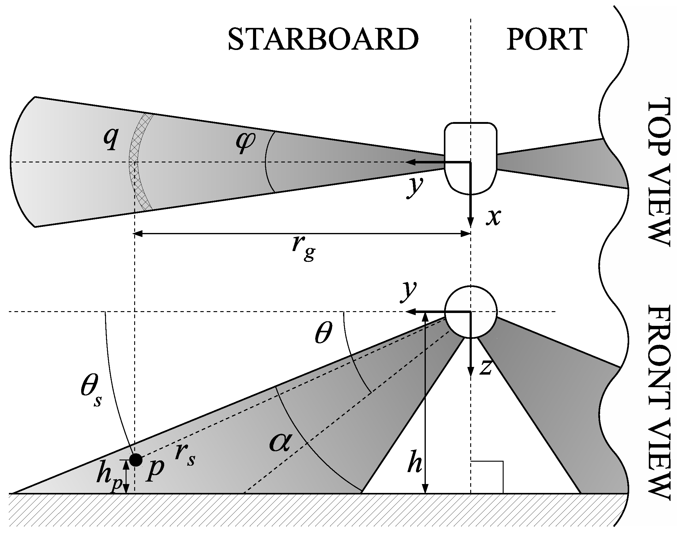
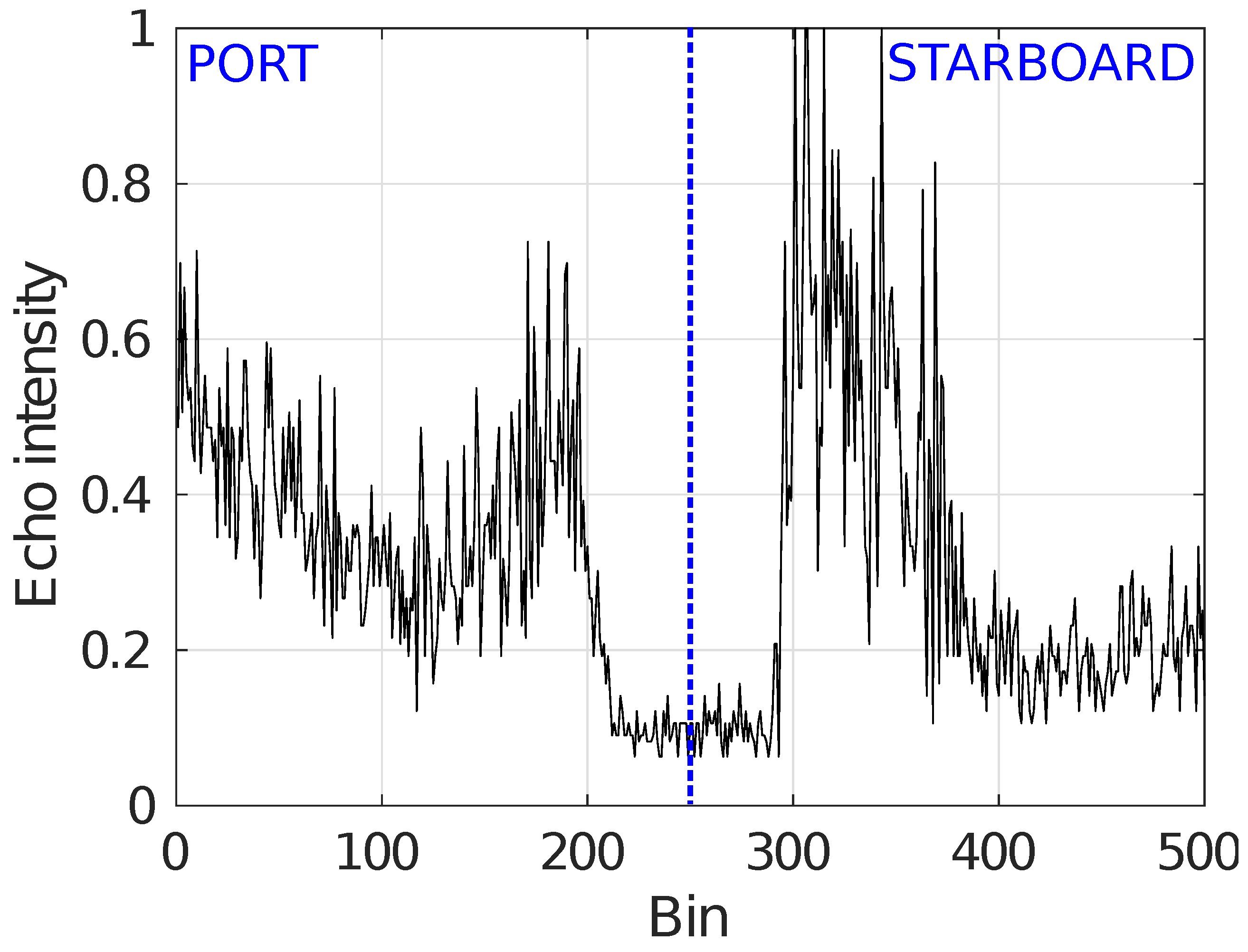
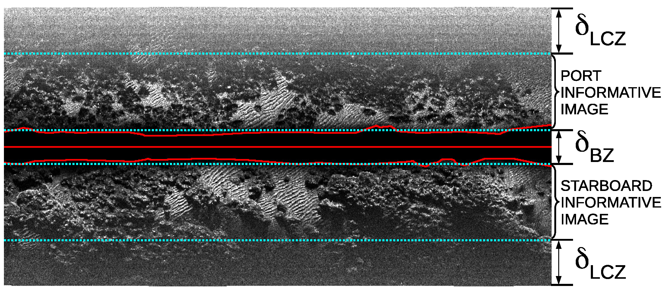
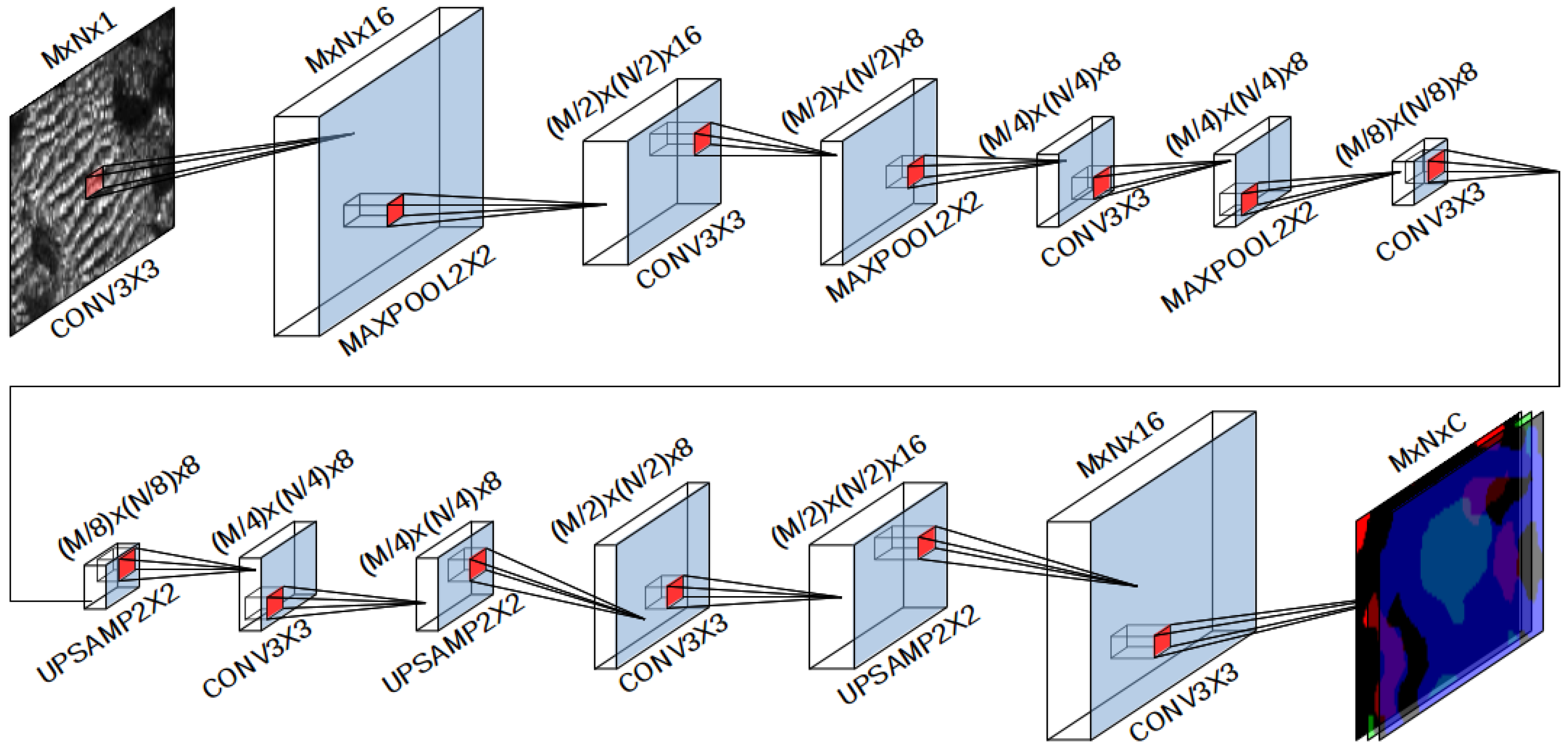
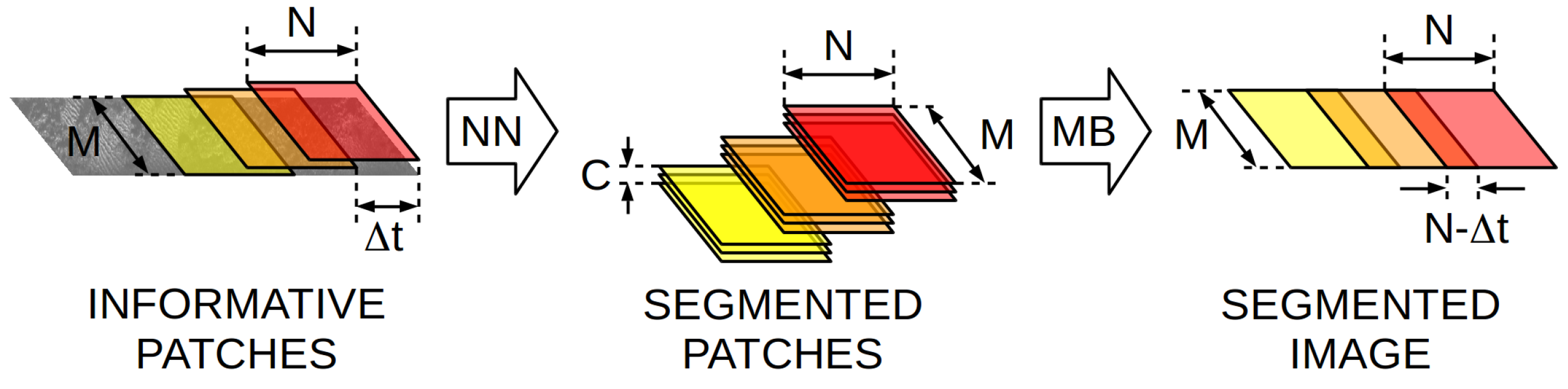
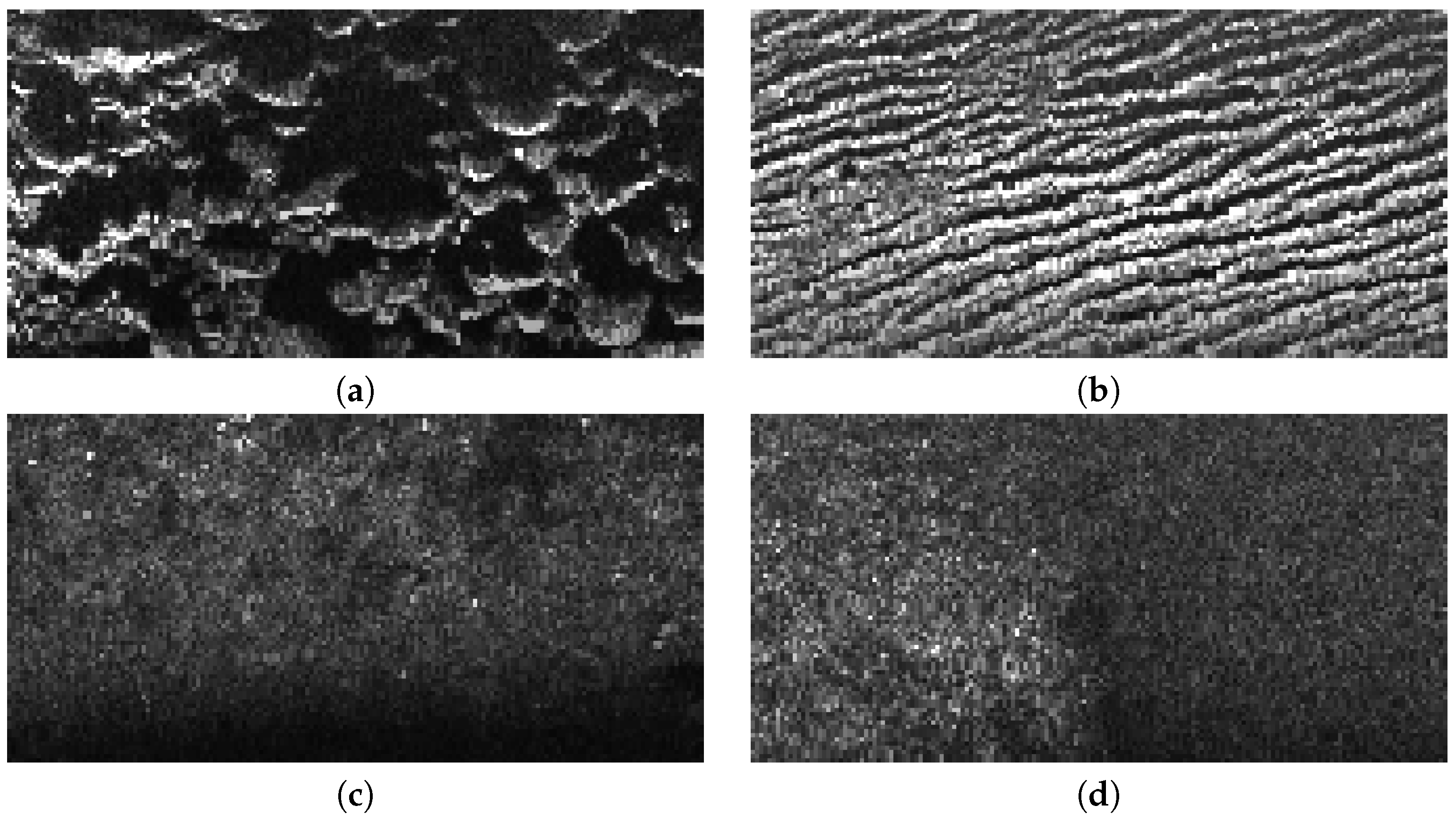
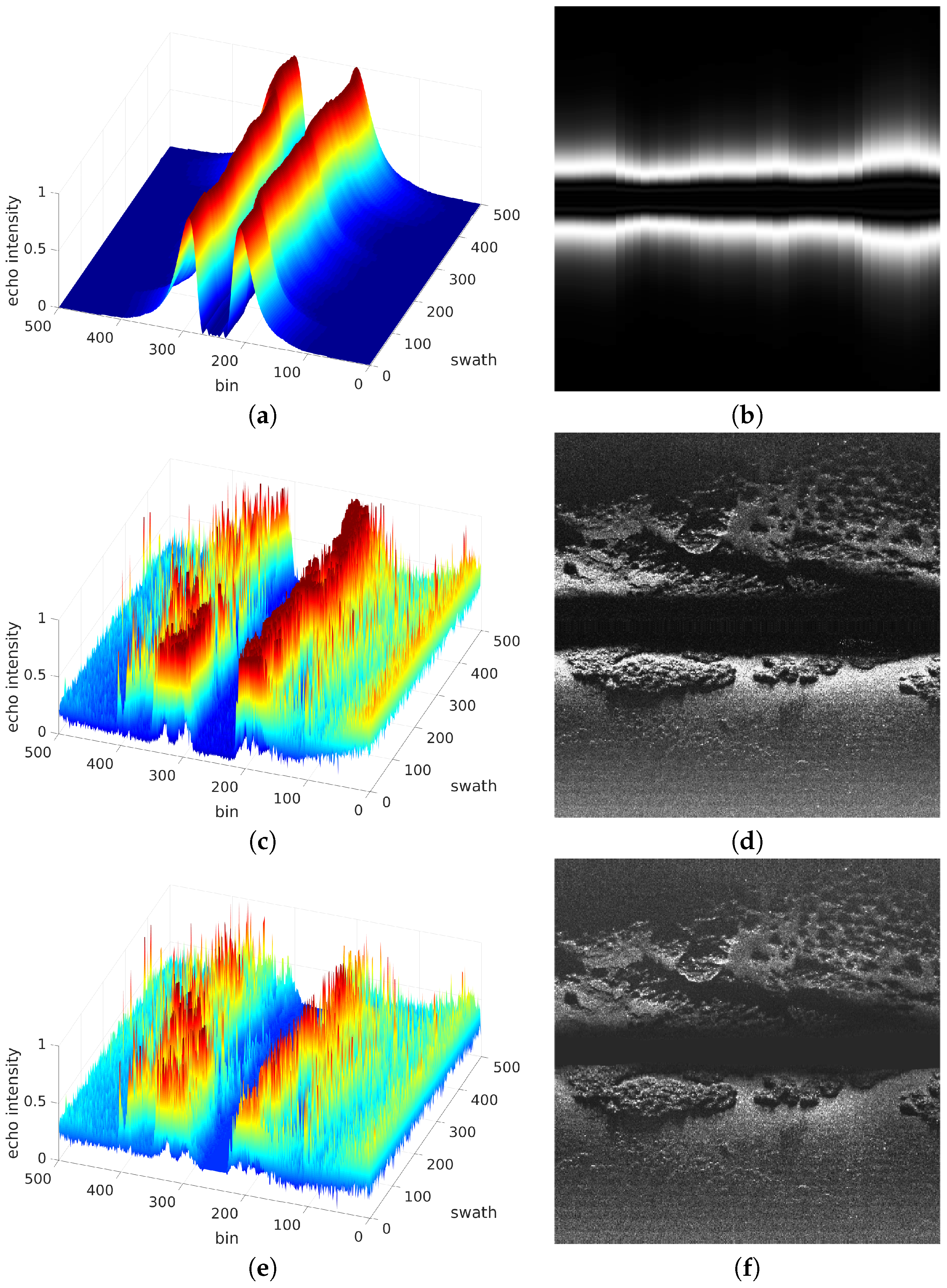
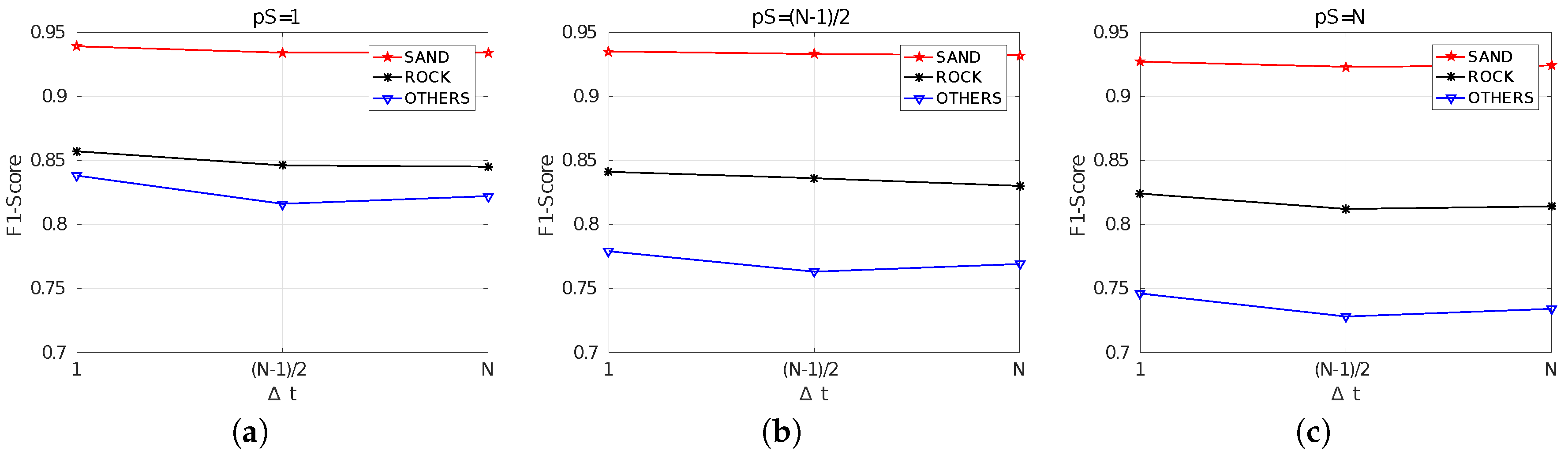
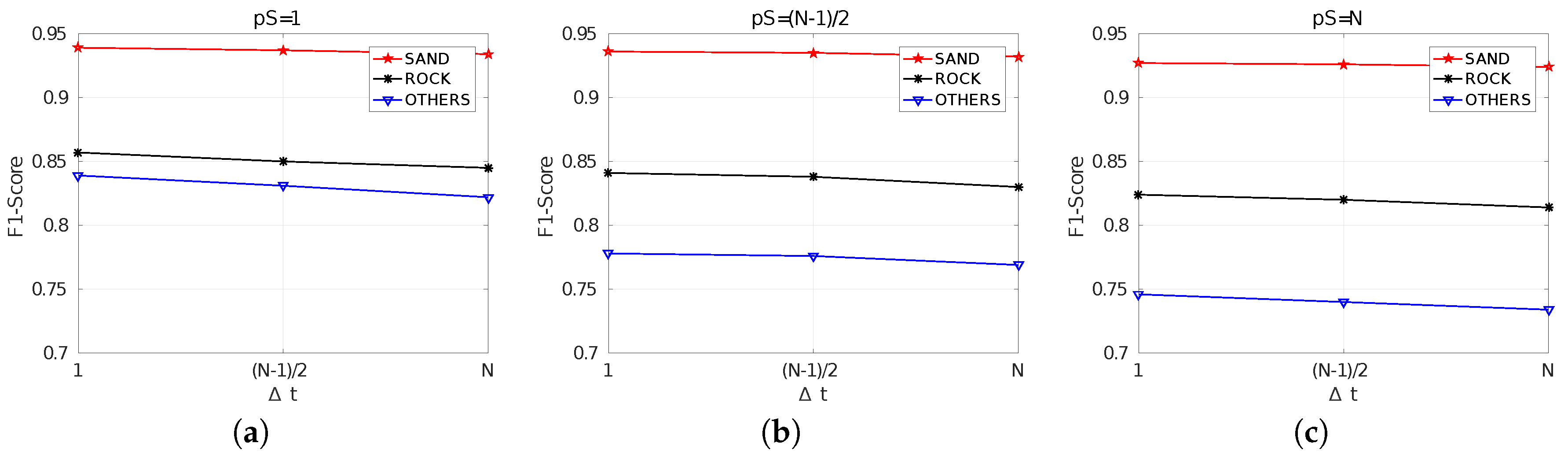
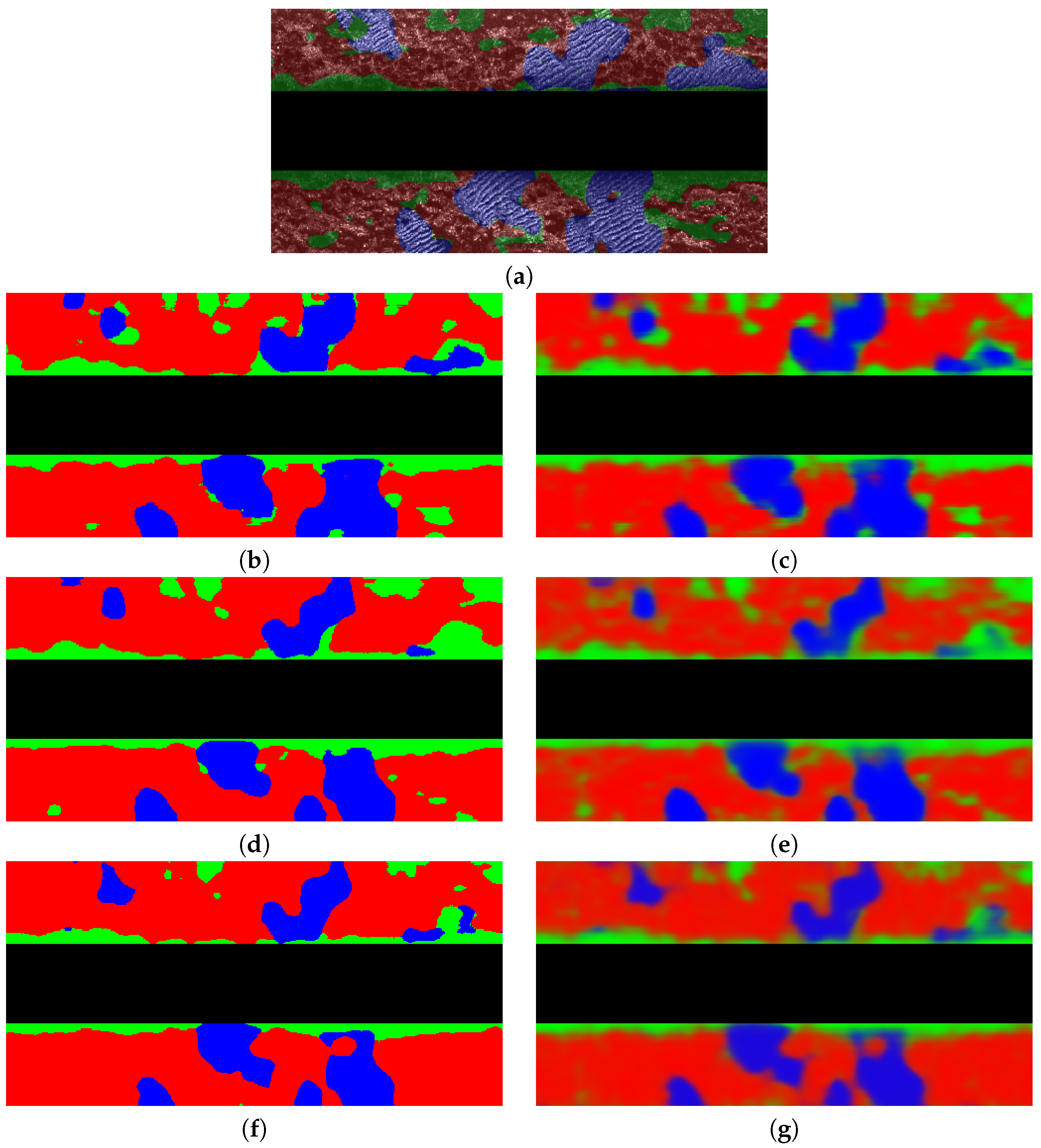
Table 1.
Parameters of the Imagenex SportScan SSS used in this paper.
| 30 | |
|---|---|
| 3 | |
| 20 | |
| f | 800 KHz |
| 1.95 mm | |
| 30 m | |
| 0.12 m | |
| Bins per swath | 250 port, 250 starboard |
| Sampling frequency | 10 swath/s |
Table 2.
Dataset specification. The number of informative bins of each class and the corresponding percentage, within parenthesis, are provided.
Table 2.
Dataset specification. The number of informative bins of each class and the corresponding percentage, within parenthesis, are provided.
| Transect | Swaths | Rock | Sand | Other |
|---|---|---|---|---|
| 1 | 5764 | 125,294 (13.095%) | 26,464 (2.766%) | 805,066 (84.139%) |
| 2 | 6800 | 107,706 (9.542%) | 133,665 (11.841%) | 887,429 (78.617%) |
| 3 | 3825 | 253,029 (39.850%) | 111,411 (17.546%) | 270,510 (42.603%) |
| 4 | 3517 | 215,148 (36.852%) | 70,604 (12.093%) | 298,070 (51.055%) |
| 5 | 2532 | 136,762 (32.538%) | 38,650 (9.196%) | 244,900 (58.266%) |
| GLOBAL | 22,438 | 837,939 (22.497%) | 380,794 (10.223%) | 2,505,975 (67.280%) |
Table 3.
Confusion matrices for SCM normalized (a) column-wise (b) row-wise.
| (a) | ||||
|---|---|---|---|---|
| True | Rock | Sand | Other | |
| Pred. | ||||
| Rock | 0.7917 | 0.0347 | 0.0428 | |
| Sand | 0.1625 | 0.9409 | 0.1308 | |
| Other | 0.0457 | 0.0242 | 0.8263 | |
| (b) | ||||
| True | Rock | Sand | Other | |
| Pred. | ||||
| Rock | 0.8803 | 0.1022 | 0.0174 | |
| Sand | 0.0602 | 0.9221 | 0.0177 | |
| Other | 0.1111 | 0.1558 | 0.7331 | |
Table 4.
Confusion matrices for MCM normalized (a) column-wise (b) row-wise.
| (a) | ||||
|---|---|---|---|---|
| True | Rock | Sand | Other | |
| Pred. | ||||
| Rock | 0.8015 | 0.0367 | 0.0461 | |
| Sand | 0.1554 | 0.9399 | 0.1358 | |
| Other | 0.0430 | 0.0233 | 0.8180 | |
| (b) | ||||
| True | Rock | Sand | Other | |
| Pred. | ||||
| Rock | 0.8721 | 0.1085 | 0.0193 | |
| Sand | 0.0563 | 0.9247 | 0.0189 | |
| Other | 0.1021 | 0.1502 | 0.7476 | |
Table 5.
Accuracy results for SCM and MCM.
| ACCURACY (SCM) | ||||
|---|---|---|---|---|
| 1 | ||||
| pS | ||||
| 1 | 0.9100 | 0.9020 | 0.9020 | |
| 0.8990 | 0.8950 | 0.8930 | ||
| 0.8830 | 0.8770 | 0.8790 | ||
| ACCURACY (MCM) | ||||
| 1 | ||||
| pS | ||||
| 1 | 0.9100 | 0.9070 | 0.9020 | |
| 0.8990 | 0.8970 | 0.8930 | ||
| 0.8840 | 0.8820 | 0.8790 | ||
Table 6.
Precision, recall, fall-out and F1-Score results when using SCM.
| Precision | ||||||||||
|---|---|---|---|---|---|---|---|---|---|---|
| 1 | ||||||||||
| PS | Rock | Sand | Other | Rock | Sand | Other | Rock | Sand | Other | |
| 1 | 0.8860 | 0.9350 | 0.7960 | 0.9050 | 0.9250 | 0.7430 | 0.8720 | 0.9320 | 0.7780 | |
| 0.8560 | 0.9370 | 0.7430 | 0.8770 | 0.9310 | 0.6960 | 0.8430 | 0.9360 | 0.7240 | ||
| 0.8950 | 0.9030 | 0.7290 | 0.9080 | 0.8970 | 0.6740 | 0.8810 | 0.9030 | 0.7150 | ||
| Recall | ||||||||||
| 1 | ||||||||||
| PS | Rock | Sand | Other | Rock | Sand | Other | Rock | Sand | Other | |
| 1 | 0.8300 | 0.9420 | 0.8850 | 0.7940 | 0.9430 | 0.9030 | 0.8190 | 0.9360 | 0.8710 | |
| 0.8270 | 0.9340 | 0.8190 | 0.8000 | 0.9360 | 0.8450 | 0.8170 | 0.9290 | 0.8190 | ||
| 0.7630 | 0.9510 | 0.7640 | 0.7340 | 0.9510 | 0.7910 | 0.7570 | 0.9470 | 0.7530 | ||
| Fall-Out | ||||||||||
| 1 | ||||||||||
| PS | Rock | Sand | Other | Rock | Sand | Other | Rock | Sand | Other | |
| 1 | 0.0340 | 0.1310 | 0.0230 | 0.0280 | 0.1480 | 0.0290 | 0.0380 | 0.1390 | 0.0250 | |
| 0.0420 | 0.1310 | 0.0290 | 0.0370 | 0.1410 | 0.0340 | 0.0460 | 0.1350 | 0.0310 | ||
| 0.0320 | 0.1810 | 0.0310 | 0.0280 | 0.1890 | 0.0370 | 0.0360 | 0.1830 | 0.0330 | ||
| F1-Score | ||||||||||
| 1 | ||||||||||
| PS | Rock | Sand | Other | Rock | Sand | Other | Rock | Sand | Other | |
| 1 | 0.8570 | 0.9390 | 0.8380 | 0.8460 | 0.9340 | 0.8160 | 0.8450 | 0.9340 | 0.8220 | |
| 0.8410 | 0.9350 | 0.7790 | 0.8360 | 0.9330 | 0.7630 | 0.8300 | 0.9320 | 0.7690 | ||
| 0.8240 | 0.9270 | 0.7460 | 0.8120 | 0.9230 | 0.7280 | 0.8140 | 0.9240 | 0.7340 | ||
Table 7.
Precision, recall, fall-out and F1-Score results when using MCM. The gray cells denote the configurations under which MCM surpasses SCM.
Table 7.
Precision, recall, fall-out and F1-Score results when using MCM. The gray cells denote the configurations under which MCM surpasses SCM.
| Precision | ||||||||||
|---|---|---|---|---|---|---|---|---|---|---|
| 1 | ||||||||||
| PS | Rock | Sand | Other | Rock | Sand | Other | Rock | Sand | Other | |
| 1 | 0.8870 | 0.9360 | 0.7950 | 0.8780 | 0.9340 | 0.7890 | 0.8720 | 0.9320 | 0.7780 | |
| 0.8550 | 0.9380 | 0.7400 | 0.8520 | 0.9370 | 0.7370 | 0.8430 | 0.9360 | 0.7240 | ||
| 0.8930 | 0.9040 | 0.7280 | 0.8880 | 0.9040 | 0.7230 | 0.8810 | 0.9030 | 0.7150 | ||
| Recall | ||||||||||
| 1 | ||||||||||
| PS | Rock | Sand | Other | Rock | Sand | Other | Rock | Sand | Other | |
| 1 | 0.8300 | 0.9420 | 0.8870 | 0.8240 | 0.9400 | 0.8780 | 0.8190 | 0.9360 | 0.8710 | |
| 0.8280 | 0.9340 | 0.8210 | 0.8260 | 0.9320 | 0.8190 | 0.8170 | 0.9290 | 0.8190 | ||
| 0.7650 | 0.9510 | 0.7650 | 0.7620 | 0.9490 | 0.7590 | 0.7570 | 0.9470 | 0.7530 | ||
| Fall-Out | ||||||||||
| 1 | ||||||||||
| PS | Rock | Sand | Other | Rock | Sand | Other | Rock | Sand | Other | |
| 1 | 0.0330 | 0.1310 | 0.0230 | 0.0360 | 0.1340 | 0.0240 | 0.0380 | 0.1390 | 0.0250 | |
| 0.0420 | 0.1300 | 0.0290 | 0.0430 | 0.1320 | 0.0300 | 0.0460 | 0.1350 | 0.0310 | ||
| 0.0330 | 0.1790 | 0.0310 | 0.0340 | 0.1800 | 0.0320 | 0.0360 | 0.1830 | 0.0330 | ||
| F1-Score | ||||||||||
| 1 | ||||||||||
| PS | Rock | Sand | Other | Rock | Sand | Other | Rock | Sand | Other | |
| 1 | 0.8570 | 0.9390 | 0.8390 | 0.8500 | 0.9370 | 0.8310 | 0.8450 | 0.9340 | 0.8220 | |
| 0.8410 | 0.9360 | 0.7780 | 0.8380 | 0.9350 | 0.7760 | 0.8300 | 0.9320 | 0.7690 | ||
| 0.8240 | 0.9270 | 0.7460 | 0.8200 | 0.9260 | 0.7400 | 0.8140 | 0.9240 | 0.7340 | ||
Table 8.
Training and segmentation time consumption when using SCM and MCM.
| Time consumption (SCM) | |||||||
|---|---|---|---|---|---|---|---|
| 1 | |||||||
| PS | Training | Segment. | Training | Segment. | Training | Segment. | |
| 1 | 1373.2110 ms | 3.2084 ms | 1373.2110 ms | 0.2174 ms | 1373.2110 ms | 0.2148 ms | |
| 36.0540 ms | 3.2304 ms | 36.0540 ms | 0.2295 ms | 36.0540 ms | 0.2294 ms | ||
| 18.0790 ms | 3.3044 ms | 18.0790 ms | 0.2323 ms | 18.0790 ms | 0.2145 ms | ||
| Time consumption (MCM) | |||||||
| 1 | |||||||
| PS | Training | Segment. | Training | Segment. | Training | Segment. | |
| 1 | 1373.2110 ms | 3.8411 ms | 1373.2110 ms | 0.6879 ms | 1373.2110 ms | 0.6580 ms | |
| 36.0540 ms | 3.8038 ms | 36.0540 ms | 0.6799 ms | 36.0540 ms | 0.6163 ms | ||
| 18.0790 ms | 3.7451 ms | 18.0790 ms | 0.6960 ms | 18.0790 ms | 0.6328 ms | ||
© 2020 by the authors. Licensee MDPI, Basel, Switzerland. This article is an open access article distributed under the terms and conditions of the Creative Commons Attribution (CC BY) license (http://creativecommons.org/licenses/by/4.0/).
Share and Cite
MDPI and ACS Style
Burguera, A.; Bonin-Font, F. On-Line Multi-Class Segmentation of Side-Scan Sonar Imagery Using an Autonomous Underwater Vehicle. J. Mar. Sci. Eng. 2020, 8, 557. https://doi.org/10.3390/jmse8080557
AMA Style
Burguera A, Bonin-Font F. On-Line Multi-Class Segmentation of Side-Scan Sonar Imagery Using an Autonomous Underwater Vehicle. Journal of Marine Science and Engineering. 2020; 8(8):557. https://doi.org/10.3390/jmse8080557
Chicago/Turabian StyleBurguera, Antoni, and Francisco Bonin-Font. 2020. "On-Line Multi-Class Segmentation of Side-Scan Sonar Imagery Using an Autonomous Underwater Vehicle" Journal of Marine Science and Engineering 8, no. 8: 557. https://doi.org/10.3390/jmse8080557
Note that from the first issue of 2016, this journal uses article numbers instead of page numbers. See further details here.