Energy Balances and Greenhouse Gas Emissions of Agriculture in the Shihezi Oasis of China

1
State Key Laboratory of Grassland Agro-Ecosystems, Key Laboratory of Grassland Livestock Industry Innovation, Ministry of Agriculture, Lanzhou 730020, Gansu, China
2
College of Pastoral Agriculture Science and Technology, Lanzhou University, Lanzhou 730000, Gansu, China
3
College of Information and Science Technology, Gansu Agricultural University, Lanzhou 730070, Gansu, China
4
Xinjiang Western Animal Husbandry Limited Company, Shihezi 832000, Xinjiang, China
*
Author to whom correspondence should be addressed.
Atmosphere 2020, 11(8), 781; https://doi.org/10.3390/atmos11080781
Submission received: 1 June 2020
/
Revised: 10 July 2020
/
Accepted: 12 July 2020
/
Published: 24 July 2020
(This article belongs to the Special Issue Greenhouse Gas Emission Mitigation: Feasibility and Economics)
Abstract
:The objective of this study was to evaluate the difference of crop and livestock products regarding energy balances, greenhouse gas (GHG) emissions, carbon economic efficiency, and water use efficiency using a life cycle assessment (LCA) methodology on farms in three sub-oases within the Shihezi Oasis of China. The three sub-oases were selected within the Gobi Desert, at Shizongchang (SZC), Xiayedi (XYD), and Mosuowan (MSW), to represent the various local oasis types: i. Oasis; ii. overlapping oasis-desert; and iii. Gobi oasis. The results indicated that crop production in XYD Oasis had higher energy balances (221.47 GJ/ha), and a net energy ratio (5.39), than in the other two oases (p < 0.01). The production of 1 kg CW of sheep in XYD Oasis resulted in significantly higher energy balances (18.31 MJ/kg CW), and an energy ratio (2.21), than in the other two oases (p < 0.01). The water use efficiency of crop production in the SZC Oasis was lower than that of the XYD and MSW oases (p < 0.05). Alfalfa production generated the lowest CO2-eq emissions (8.09 Mg CO2-eq/ha. year) and had the highest water use efficiency (45.82 MJ/m3). Alfalfa (1.18 ¥/kg CO2-eq) and maize (1.14 ¥/kg CO2-eq) had a higher carbon economic efficiency than other crops (p < 0.01). The main sources of GHG emissions for crop production were fertilizer and irrigation. The structural equation modelling (SEM) of agricultural systems in the Shihezi Oasis showed that the livestock category significantly influenced the economic income, energy, and carbon balances.
1. Introduction
The typical Shihezi meta-ecosystem of mountains, oases, and desert in northwest China consists of Tianshan Mountain, Shihezi Oasis, and the Gurbantunggut Desert. The areas of the mountain, oasis, and desert in this ecosystem are 2541 km2, 7681 km2, and 10,996 km2, respectively [1]. The Manasi River is the lifeblood of the Shihezi Oasis. It originates from Tianshan Mountain and runs dry in the Gurbantunggut Desert. Agricultural production in the Shihezi Oasis is located in three sub-oases: Shizongchang (SZC), Xiayedi (XYD), and Mosuowan (MSW). More than 95% of people, farm produce, and energy production are concentrated in these sub-oases. At present, many problems such as secondary salinization of cropland, desertification, chemical pollution, and climate change have seriously threatened the sustainability of oasis agriculture through a lack of knowledge and understanding of oasis agricultural management [2]. There exists a close relationship between agricultural production and energy use [3]. Agricultural production requires high human-applied energy inputs, of which a large proportion are imported (i.e., fertilizer, diesel, electricity, pesticide, etc.), the remaining being produced on farms as bio-energy (i.e., seed, manure, and animate energy provided by living plants in nature). Crop yields can be improved (i.e., at economic maximum) by increasing the net energy (outputs/inputs) of crops [4].
Since 1950, the average rate of increase in global temperatures has been 0.17 °C per decade due to agricultural practices [5]. Agriculture has been considered as a major contributor to GHG emissions [6]. Crop yields in developing countries are projected to decrease due to global climate change [7]. As elsewhere, there are enormous challenges of alleviating greenhouse gas (GHG) emissions from agricultural production due to the heterogeneous nature and biophysical complexity of farming systems in China [8].
Characterizing the energy balances and GHG emissions of agricultural practices in the Shihezi Oasis offer key information to mitigate carbon emissions and ensure food security [6]. Energy consumption and GHG emissions involve on-farm and off-farm inputs, which are carbon-based operations and products [8]. In this study, the system boundary and scope of calculating energy balances and GHG emissions only included farm agricultural production practices using the life cycle assessment (LCA) methodology. The objectives of this study were to calculate the differences of energy balances and GHG emissions from various oasis ecotypes (SZC vs. XYD vs. MSW) in the Shihezi Oasis associated with producing per unit of crop and livestock products using the LCA technique. Moreover, finding the difference in energy balance and GHG emissions between six crops and water use efficiency of crop production in the Shihezi Oasis was the other aim of this study.
2. Materials and Methods
2.1. Study Site
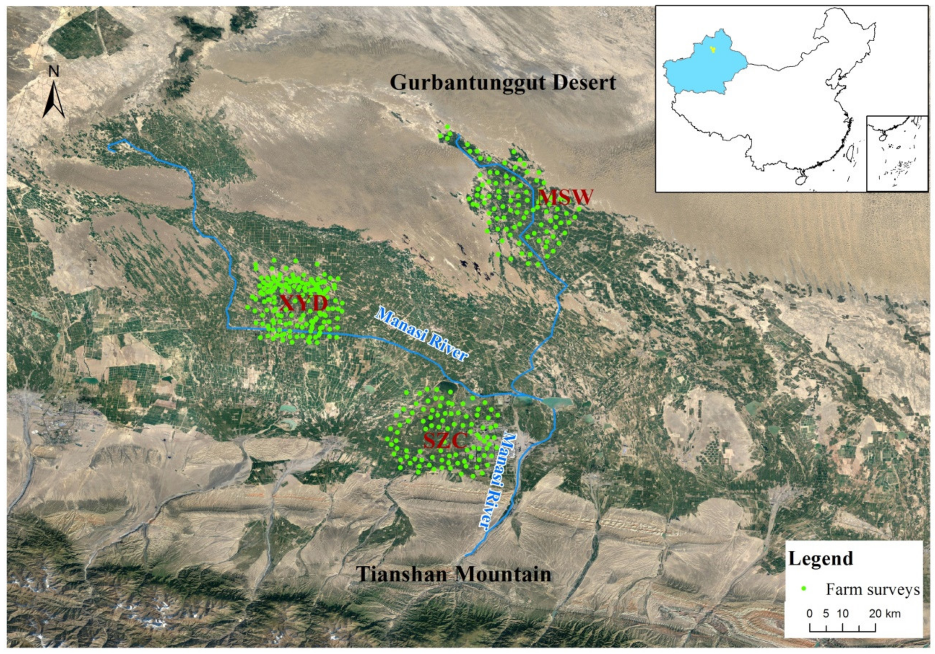
Shihezi Oasis, which is divided into the three sub-oases, the SZC, XYD, and MSW oases, is located in the center of the northern foothills of Tianshan Mountain in XinJiang, China (84°58′–86°64′ E, 43°26′–45°20′ N, Figure 1 and Figure S1). Agricultural production in the Shihezi Oasis is divided geographically into three contrasting systems (Figure 1 and Figure S1):
- (a)
- SZC sub-oasis, with a total area of 37.58 × 10³ ha, of which 20.5 × 10³ ha is cultivated, sits on an inclined piedmont plain. The Manasi River winds its way through the northeast of the sub-oasis; other surface and groundwater sources are abundant, and in a rural zone of Shihezi City, a freshwater spring overflow is used for flood (border dyke) irrigation;
- (b)
- XYD sub-oasis, with a total area of 300 × 103 ha, of which 61 × 103 ha is cultivated, lies where the Manasi River downstream oasis system and Gurban Tunggut Desert overlap;
- (c)
- MSW sub-oasis, with a total area of 137 × 103 ha, of which 44 × 103 ha is cultivated, lies where the Manasi River allows the sub-oasis to cut through the Gurban Tunggut Desert for a distance of 60 km.
2.2. Data Collection
Data were collected from official records, published literature, and farm survey data. The farm surveys were carried out from 2015 to 2016 with a selection of a random 354 farmers in this study (Tables S1 and S2). Inputs of crop production comprised of labor, seed, fertilizer, pesticide, fuel and electricity consumption, plastic film, and the life and working hours of farm machines. Outputs of crop production accounted as crop products including grain, straw, and roots. Inputs of livestock production were comprised of labor, feed (intake, source, and processing), and fuel and electricity consumption. Outputs of livestock production only included livestock products (carcass weight, milk, and wool). To quantify the GHG emissions from livestock production, data from livestock production included categories, livestock numbers, age, feed sources, and feed usage. Structural equation modelling (SEM) can evaluate direct and indirect effects between variables by expected statistical relationships. An SEM analysis program named AMOS 19.0 (IBM Corporation, New York, USA) was used to evaluate the direct and indirect effects of predictor variables on net income, energy balances, and carbon balances. A good fit for that model is 0 ≤ χ2/df ≤ 2 and 0.05 < p ≤ 1 [9].
2.3. Goal and Scope Definition
Based on the ISO standard, the overall goal and scope of this study was to evaluate energy balances and GHG emissions on farms [10]. The specific aim was to quantify the sustainability impacts associated with energy balances and GHG emissions per ha of cropland and kg of livestock products between three sub-oases in Shihezi of China. The target audience included the farm and its stakeholders, consumers, and the public.
2.4. Functional Unit
The functional unit was defined for the purposes of this study, with GJ/ha for carbon balances of crop production and MJ/kg of carcass weight (CW) and milk for carbon balances of livestock. Based on information from the global warming potential for a 100-year period, the data of CH4 and N2O emissions were converted into CO2 equivalents, with 34 for CH4 and 298 for N2O. The units of GHG emissions were kg CO2-eq/ha for cropland, kg CO2-eq/kg for crop products, and kg CO2-eq/kg CW and milk for livestock products.
2.5. Calculation of Energy Balances
The human-applied energy inputs of crop production are calculated as Equation (1).
where EIcrop is the unit area of total energy inputs for crop production (MJ/ha), CI is the unit area of energy input for crop production, and EC is the energy coefficient (Table 1). In regards to indexing, l, s, f, p, ie, pm, dc, and md are inputs of human labor (h), seed (kg), fertilizers (kg), pesticides (kg), electricity consumption for irrigation (kwh), and plastic films (kg), respectively. The energy outputs for each category of crop including the grain, straw, and roots are calculated as Equation (2).
where EOcrop is the unit area of total energy outputs from crop products (MJ/ha) and CY is the unit area of yield. In regards to indexing, grain, straw, and root are grain (kg), straw (kg), and roots (kg) of crop products, respectively.
The energy inputs of livestock production are calculated as Equation (3).
where EIlivestock is the unit carcass (milk) weight of total energy inputs for livestock production (MJ/kg CW and milk), LI is the unit livestock of energy input for livestock production, and CWlivestock is the unit livestock of carcass weight (i.e., the weight of meat with bone except for fur, viscera, head, hooves, and blood). In regards to indexing, feed, drug, labor, elec, coal, j, and m are feed inputs (kg), veterinary drugs (kg), human labor (h), electricity consumption for lighting of livestock housing (kwh), coal consumption for heating of livestock housing in winter (kg), feed classified j, and feed types, respectively.
The energy outputs of livestock products are calculated as Equation (4).
where EOlivestock is the unit carcass (milk) weight of total energy outputs from livestock products (MJ/kg CW and milk) and LY is the unit livestock of yield. In regards to indexing, carcass, milk, and wool are carcass weight (kg), milk (kg), and wool of livestock (kg), respectively.
The energy indices of balances and ratios are calculated as follows:
where EBcrop&livestock represents the energy balances of crops (MJ/ha) or livestock (MJ/CW and milk). NERcrop&livestock represents the net energy ratio (output/input) of crop or livestock production. EOcrop&livestock and EIcrop&livestock represent the same parameters of the above equation, respectively.
2.6. Calculation of GHG Emissions
The GHG emissions for each category of crop production input are calculated as Equation (7).
where CEcrop is the unit area of GHG emissions (kg CO2-eq/ha) and EF is the emission factor (Table 2). SOILres is the unit area of GHG emissions from soil respiration (kg CO2-eq/ha) using the following, Equation (8) [17].
where T, P, and SOC are the annual mean temperature (°C), the annual rainfall (m), and soil organic carbon between a 0 and 20 cm depth (kg C.m−2), respectively [10].
Carbon stocks of crop production are calculated using Equation (9) [28].
where CScrop, CSgain, CSstem, and CSroot represent the unit area of carbon values accumulated in crops (kg CO2-eq/ha), grain (kg CO2-eq/ha), stems (kg CO2-eq/ha), and roots (kg CO2-eq/ha), respectively.
Carbon balances of crop production are calculated as Equation (10).
where CBcrop represents the unit area of carbon balances (kg CO2-eq/ha).
The yearly GHG emissions from each livestock species are calculated using Equation (11).
where CElivestock is the unit carcass (milk) weight of GHG emissions from livestock (kg CO2-eq/kg CW and milk), TCO2 is the emissions of carbon dioxide, TCH4 is the emissions of methane, and TN2O is the emissions of nitrous oxide. In regards to indexing, enteric and manure are ruminant enteric fermentation (kg CO2-eq/kg CW and milk) and manure management (kg CO2-eq/kg CW and milk), respectively.
The carbon stock and carbon balances of livestock production are calculated as the following, Equations (12) and (13) [29].
where CSlivestock is the carbon stock of livestock (kg CO2-eq/kg CW and milk) and LW is the live weight of livestock. CBlivestock is the carbon balance (kg CO2-eq/kg CW and milk).
2.7. Calculation of Carbon Economic Efficiency
Based on emissions per one kilogram of carbon dioxide equivalence from agricultural products, the total carbon economic efficiency associated with the mean market price of these products in 2015 and 2016 (Table S3) is calculated using Equation (14) [28].
where CEE is the carbon economic efficiency (¥/kg CO2-eq), YP is the yield of agricultural products (kg), PRICE is the price of agricultural products (¥), and CE is the GHG emissions from agricultural production (kg CO2-eq).
2.8. Calculation of Water Use Efficiency
The analysis of energy balance per 1 cubic meter of water can find the relationship between irrigation and the net energy of crop production in the Shihezi Oasis. The water use efficiency of crop production is calculated using Equation (15):
where WUEcrop, EBcrop, and WUcrop represent the water use efficiency of crops grown (MJ/m3), energy balances (MJ/ha), and the water use of crops grown (m3/ha), respectively.
2.9. Statistical Analyses
We used the statistical program named Genstat17.0 (VSNI Corporation, Hemel Hempstead, UK) to analyze differences in energy indices (energy balances and net energy ratio), carbon indices (GHG emissions, carbon stock, carbon balances, and carbon economic efficiency), water use, and water use efficiency using inline linear models.
3. Results
3.1. Yield and Water Use of Crop Production
The results of the yield and water use of crop production in three sub-oases of the Shihezi Oasis are presented in Table 3. The yields (kg DM/ha) of maize and cotton in SZC Oasis were significantly higher than in the other two oases (p < 0.05). The water use for wheat (spring) and maize production in SZC Oasis was higher than in the other two oases (p < 0.05).
3.2. Energy Balances, Net Energy Ratio, and Water Use Efficiency of Agricultural Production
The results of energy balances, the net energy ratio, and water use efficiency in three sub-oases of Shihezi Oasis are presented in Table 4 and Table S4. For crop production, the output energy (308.69 GJ/ha), energy balances (221.47 GJ/ha), and net energy ratio (5.39) in the XYD Oasis were the highest among the three production systems; the corresponding values of MSW Oasis were higher than in the SZC Oasis, respectively (Table 4). However, the input energy (42.58 GJ/ha) in the MSW Oasis was lower than in the other two oases (p < 0.01). The net energy ratio (6.45) and energy balances (309.46 MJ/ha) of maize in the XYD Oasis were significantly higher than that of the SZC and MSW oases (Table 4). Alfalfa (12.71) and maize (6.27) had higher net energy ratios than other crops (p < 0.01) (Table S4). For livestock production, the production of 1 kg CW of sheep in XYD Oasis resulted in significantly higher energy balances than in the other two oases. Similarly, the net energy ratio (2.21) of sheep in the XYD Oasis was significantly higher than that of the SZC and MSW oases (Table 4).
3.3. GHG Emissions and Carbon Economic Efficiency of Agriculture Production
Carbon indices to evaluate agriculture production are presented in Table 5 and Table S4. Carbon balances (−1.12 Mg CO2-eq/ha) of crop production in SZC Oasis were lower than in the other two oases (p < 0.05) (Table 5). GHG emissions (17.72 Mg CO2-eq/ha) from cotton production were significantly higher than for the other five crops (p < 0.01) (Table S4). Alfalfa had higher carbon stocks (23.76 Mg CO2-eq/ha) and carbon balances (15.97 Mg CO2-eq/ha) than other crops (p < 0.01) (Table S4). According to the price of agricultural products (Table S3) and carbon input for farm production, SZC Oasis had a lower carbon economic efficiency (0.34 ¥/kg CO2-eq) of crop production than the other two oases (p < 0.05) (Table 5). The carbon economic efficiency of maize (1.14 ¥/kg CO2-eq) and alfalfa (1.18 ¥/kg CO2-eq) were significantly higher than other crops (p < 0.01) (Table S4).
3.4. Water Use Efficiency Based on Energy
Water use and the water use efficiency of crop production in the Shihezi Oasis are presented in Table 3 and Table 4. Among the three sub-oases in the Shihezi Oasis, the water use of crop production in the MSW Oasis is lower than the corresponding value of the SZC and XYD oases (p < 0.05). However, the water use efficiency of crop production in the SZC Oasis is lower than that of the XYD and MSW oases (p < 0.05). The water use (4590 m3/ha) for alfalfa production in the Shihezi Oasis is the lowest, with the highest water use efficiency (45.82 MJ/m3) (Table S4).
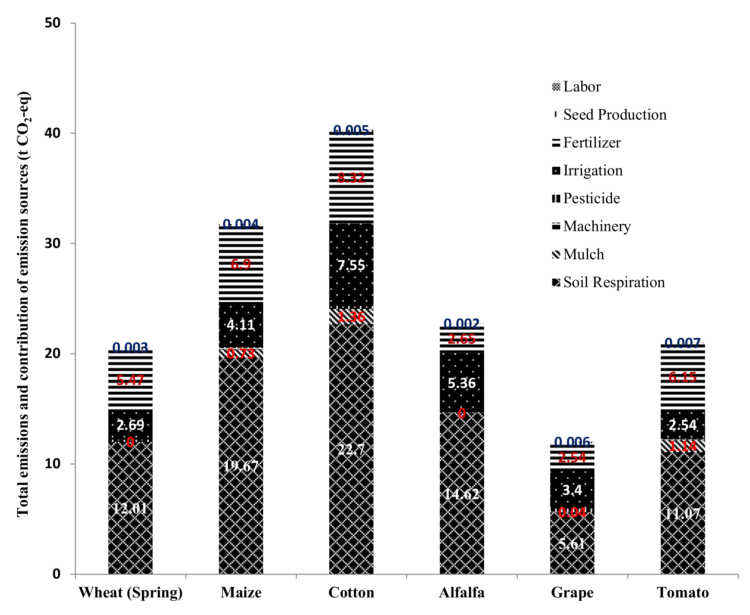
3.5. Contribution of Carbon Emissions
To further illustrate the relationship between GHG emissions and other factors, Figure 2 shows the contribution of GHG emissions from inputs of crop production. The major GHG emission sources within the crop production system are fertilizer and irrigation.
3.6. Effect Analysis of Structural Equation Modelling (SEM)
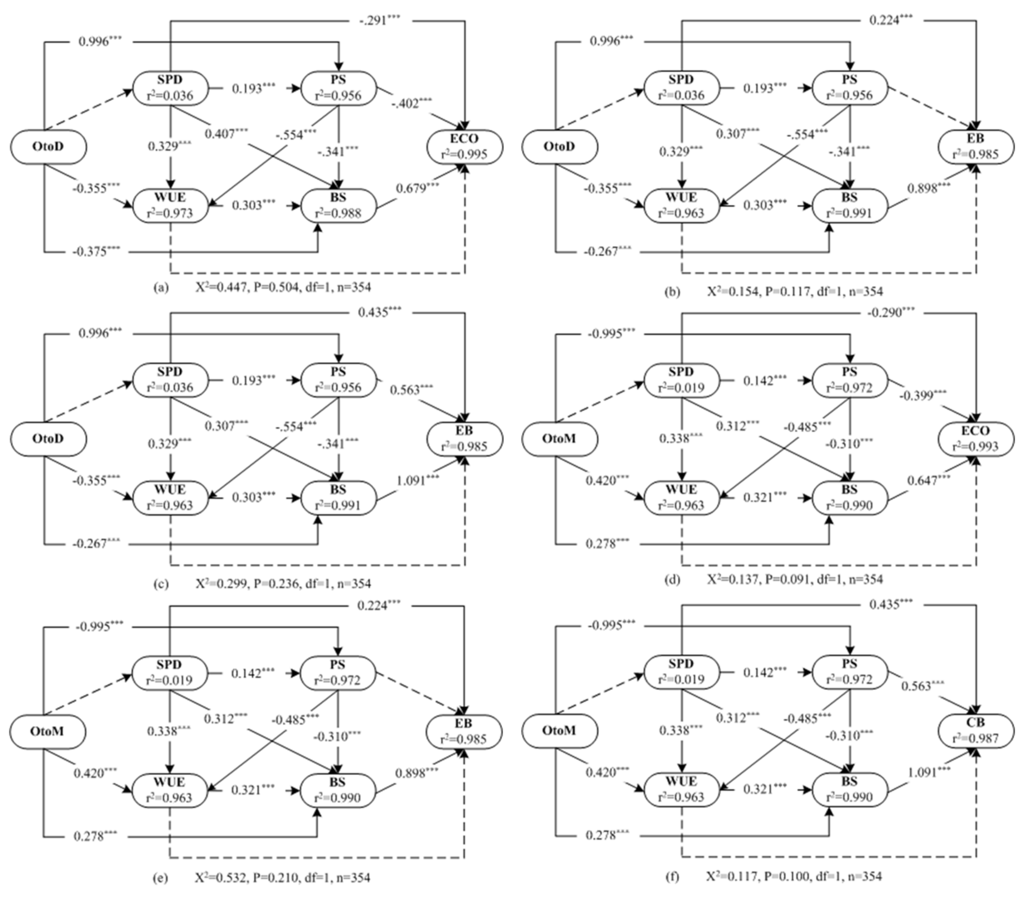
The effect analysis of SEM is presented in Table S5. The path modes show that the direct and total effects of the livestock breeding structure on predicted variables (farm net income, energy, and carbon balances) are much stronger than other dependent variables (Figure 3a, total effects = 0.647; Figure 3b, total effects = 0.898; Figure 3c, total effects = 1.091; Figure 3d, total effects = 0.980; Figure 3e, total effects = 0.898; and Figure 3f, total effects = 0.1.091). Similarly, the path modes show that the indirect effects of water use efficiency on economy income, energy, and carbon balances are much stronger than those of other variables (Figure 3a, indirect effects = 0.196; Figure 3b, indirect effects = 0.297; and Figure 3c, indirect effects = 0.430).
4. Discussion
4.1. Energy Balances and Net Energy Ratio
The present energy balances of agricultural production in the Shihezi Oasis are comparable to those published elsewhere in the world using the similar methodology of calculating the input and output energy values on farms. For example, the input energy of cotton production (58.80 GJ/ha) in the Shihezi Oasis is much higher than that (31.237 GJ/ha) in Iran [30]. This difference refers to the low energy input of weed controlling and harvesting operations using human labor instead of applying machinery in Iran. Nevertheless, Shihezi’s input energy for maize production (49.71 GJ/ha) is close to that reported in Iran (50.458 GJ/ha) due to similar intensive and high input crop production systems [31]. However, our output energy including grain, straw, and roots of maize production (341.21 GJ/ha) is much higher than that only related to grain estimated in Iran (134.946 GJ/ha) [30]. The net energy ratios of wheat and maize production in the research area are much higher than that (3.95 vs. 2.13, 6.27 vs. 2.67, respectively) in Iran [31,32]. The reason for the lower output energy and net energy ratio of crop production estimated in Iran is that the outputs included only grain. However, the net energy ratio of wheat production in this study is higher than that (3.95 vs. 1.59) in Pakistan due to less wheat yield as output energy [33]. The corresponding value of maize production in the research area is also higher than that (6.87 vs. 5.52) in Turkey due to less crop yields [34].
The flow of energy and matter is the driving force of agricultural development [35]. Agricultural production in the Shihezi Oasis is a high inputs and outputs system. With the rapid development of agriculture, high inorganic energy inputs can satisfy people’s expectations of living standards, but at the cost of environmental sustainability. From data in this research study (cf. Table S1), a more sustainable approach for Shihezi Oasis farmers would be to increase both alfalfa acreage and sheep numbers, in tandem.
4.2. GHG Emissions from Agricultural Systems
Similarly, GHG emissions from agricultural systems in the Shihezi Oasis are comparable to those evaluated in other places. For example, GHG emissions for maize production (12.1 MgCO2-eq/ha) in this study are similar to those reported in Iran (12.9 Mg CO2-eq/ha) due to similar energy inputs of maize production [31]. As the effective value of economic output produced by the unit carbon input, the signals of carbon economic efficiency can explain the benefits of carbon cost to society. The present carbon economic efficiency for wheat production ($0.027/kg CO2-eq) is higher than that ($0.023/kg CO2-eq) in the USA [36]. The most significant reason for this difference is GHG emissions from wheat production, ranging from 0.14–0.38 CO2-eq per kg of wheat produced on farms in the USA. Apart from this paper, there is no other related research on carbon balances in China which is significant enough to suggest adjusting the balance of crops with livestock production. As already stated, in the Shihezi Oasis, high inputs such as fertilizer, mulch, and machinery resulted in high outputs in crop production, but also in high GHG emissions. In addition, if GHG emissions are to be related to climate policy framework in the future, similar to legislation introduced in some other countries, it will be essential to know the impact of those polices on crop and livestock production costs.
4.3. Balance between Livestock and Forage Crops
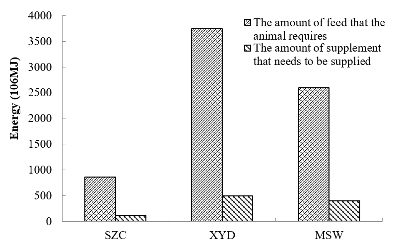
There exists an imbalance between livestock and forage crop energy inputs vs. outputs in the Shihezi Oasis (Figure 4). Livestock numbers in the Shihezi Oasis are far greater than can be supported by the forage crop supply. For example, the current forage crop supply in XYD Oasis could not meet the feed demand of livestock, which had the largest number of livestock among the three sub-oases in the Shihezi Oasis. Livestock feedstuff prices in the Shihezi Oasis, whether bought or sold, are the same (Table S2), indicating that the cost of growing feedstuff “on farm” is less than the cost of buying it from outside. This is good reason for oasis forage maize and alfalfa acreage to be greatly increased, and thus bringing the demand and supply into balance.
Similarly, the revenue (13,976 ¥/ha) of alfalfa production in 2014 was higher than that (10,275 ¥/ha) of cotton production in the oasis of the Manasi River. The differences of net income per 100 sheep in 2014 were ¥29,492 between proposed crop-livestock production compared to the current practices of Nileke County of the Xinjiang Autonomous Region in China [37]. The revenue per hectare of maize production in Dingxi City of Gansu Province in China was much higher than that (¥14,070 vs. ¥3315) of wheat production in 2018. The net income of integrated crop-livestock production in 2018 was 3.19 times that of intensive crop production [38].
4.4. Uncertainty of Energy Balances and GHG Emissions Assessment
As a basic assessment of energy balances and GHG emissions from agricultural systems in the Shihezi Oasis, there still existed many factors of uncertainty. Firstly, there were differences in data of arable land area, livestock numbers, and inputs of agricultural production within each sub-oasis. Secondly, the statistical method of partial data in China’s literature is different from that in developed countries. Thirdly, the coefficient for calculation of carbon balances and GHG emissions in the Shihezi Oasis were estimated using overseas data reported by Zeng et al. [39], and Cheng et al. [6]. In addition, the other factors such as energy consumption and GHG emissions from plastic mulch were only associated with plastic production. In this study, we only used the Tier 1 method of IPCC 2013 to evaluate GHG emissions from livestock production [11]. Nevertheless, the basic estimation of energy balances and GHG emissions in the Shihezi Oasis may offer fundamental information for the Chinese government to develop long-term agricultural policies on food security, energy conservation, and GHG emissions reduction in northwest China.
5. Conclusions
The models of energy balances, carbon balances, carbon economic efficiency, and water use efficiency developed in this study were used to calculate the differences of energy balances and GHG emissions from the three various local oasis ecotypes in the Shihezi Oasis. The evaluation indicated that crop production in the XYD Oasis had higher energy balances (221.47 GJ/ha) and an energy ratio (5.39) than in the SZC and MSW oases. The sheep production per kg of CW in the XYD Oasis had higher energy balances (18.31 MJ/kg CW) and an energy ratio (2.21) than in the other two oases. The water use efficiency of crop production in the SZC Oasis was lower than that of the other two oases (p < 0.05). These evaluation models in the present study were also used to calculate the differences of energy balances, GHG emissions, and carbon economic efficiency from local main crops in the Shihezi Oasis. We found one hectare of forage crops (i.e., alfalfa and maize) generated fewer emissions than any of the other four crops (wheat, cotton, grapes, and tomatoes). Alfalfa production in the Shihezi Oasis had the lowest water use (4594.0 m3/ha) and highest water use efficiency (45.82 MJ/m3) compared with all other five crops (wheat, maize, cotton, grapes, and tomatoes). The carbon economic efficiency of maize, relative to its market value, was significantly higher than that for each of the other five crops. Fertilizer and irrigation were the two main GHG emission sources from crop production in all three sub-oases together. Analysis of SEM showed that the livestock breeding structure and water use efficiency significantly influenced farm income, and energy and carbon balances in the Shihezi Oasis. The agro-system of Shihezi Oasis was dominated by crop production derived by high energy inputs (e.g., irrigation, fertilizer, and pesticide). The present production model of Shihezi Oasis will bring high risk to the environment and market. However, integrated crop-livestock production will increase energy use efficiency and decrease GHG emissions from the agriculture system in the Shihezi Oasis. A more sustainable approach for the agricultural development of Shihezi Oasis would be to increase both forage crop (i.e., alfalfa and maize) acreage and sheep numbers, in tandem.
Supplementary Materials
The following are available online at https://www.mdpi.com/2073-4433/11/8/781/s1, Figure S1: Longitudinal section of Shihezi study site to show Mountain-Oasis-Desert coupling ecological system (84°58′–86°64′ E), Table S1: Average data of climate, crop, and livestock of the three sub-oases in the Shihezi Oasis (2015–2016), Table S2: The structured questionnaire of farm survey, Table S3: Average market price of inputs and outputs for agricultural production (2015–2016), Table S4: Energy balances, carbon balances, carbon economic efficiency, water use, and water use efficiency of crop grown in the Shihezi Oasis, Table S5: The standardized direct, indirect and total effects between dependent variables and predict variables.
Author Contributions
F.H. (Fujiang Hou) and Z.Y. conceived and designed the experiments; F.H. (Fuqin Hou) and Z.Y. performed the experiments and farm survey; Z.Y. and F.H. (Fuqin Hou) analyzed the data; Z.Y. wrote the main manuscript text; and F.H. (Fujiang Hou) reviewed the manuscript. All authors have read and agreed to the published version of the manuscript.
Funding
This research was funded by the National Natural Science Foundation of China (No. 31660347 and 31172249), the National Key Project of Scientific and Technical Supporting Programs (No. 2014CB138706), and Programme for Changjiang Scholars and University Innovation and Research Teams (No. IRT13019).
Acknowledgments
The authors thank Roger Davies (NZCFS) for his support in fruitful discussion.
Conflicts of Interest
The authors declare no conflict of interest.
References
- Ren, J.Z.; He, D.H.; Wang, N.; Zhu, X.Y.; Li, Z.Q. Models of coupling agro-grassland systems in desert-oasis region. Acta Prataculturae Sin. 1995, 2, 11–19. (In Chinese) [Google Scholar]
- Kramer, K.J.; Moll, H.C.; Nonhebel, S. Total greenhouse gas emissions related to the Dutch crop production system. Agric. Ecosyst. Environ. 1999, 72, 9–16. [Google Scholar] [CrossRef]
- Ozkan, B.; Akcaoz, H.; Fert, C. Energy input–output analysis in Turkish agriculture. Renew. Energy 2004, 29, 39–51. [Google Scholar] [CrossRef]
- Khoshnevisan, B.; Rafiee, S.; Omid, M.; Mousazadeh, H.; Rajaeifar, M.A. Application of artificial neural networks for prediction of output energy and GHG emissions in potato production in Iran. Agric. Syst. 2014, 123, 120–127. [Google Scholar] [CrossRef]
- Lal, R. Carbon emission from farm operations. Environ. Int. 2004, 30, 981–990. [Google Scholar] [CrossRef] [PubMed]
- Cheng, K.; Pan, G.; Smith, P.; Luo, T.; Li, L.; Zheng, J.; Zhang, X.; Han, X.; Yan, M. Carbon footprint of China’s crop production—An estimation using agro-statistics data over 1993–2007. Agric. Ecosyst. Environ. 2011, 142, 231–237. [Google Scholar] [CrossRef]
- Broad, K.; Agrawala, S. The ethiopia food crisis-uses and limits of climate forecasts. Science 2000, 289, 1693–1694. [Google Scholar] [CrossRef]
- Marland, G.; West, T.; Schlamadinger, B.; Canella, L. Managing soil organic carbon in agriculture: The net effect on greenhouse gas emissions. Tellus B 2003, 613–621. [Google Scholar] [CrossRef]
- Yan, Z.G.; Li, W.; Yan, T.H.; Chang, S.H.; Hou, F.J. Evaluation of energy balances and greenhouse gas emissions from different agricultural production systems in Minqin Oasis, China. PeerJ 2019, 7, e6890. [Google Scholar] [CrossRef] [Green Version]
- International Organization for Standardization. ISO14044: Environmental Management—Life Cycle Assessment—Requirements and Guidelines; ISO: Geneva, Switzerland, 2006; pp. 1–16. [Google Scholar]
- Intergovernmental Panel on Climate Change (IPCC). Climate Change 2014: Mitigation of Climate Change. Available online: http://www.ipcc.ch/report/ar5/wg3/ (accessed on 21 July 2020).
- Wen, D.; Pimentel, D. Energy flow through an organic agroecosystem in China. Agric. Ecosyst. Environ. 1984, 11, 145–160. [Google Scholar] [CrossRef]
- Pimentel, D. Handbook of Energy Utilization in Agriculture; Bender, M., Ed.; CRC Press: Boca Raton, FL, USA, 1980; pp. 155–161. [Google Scholar]
- Huang, Z.W.; Yang, D.G.; Li, X.P.; Refu, K.T. Analysis on the energy flow of the farmer households and the characteristics of the eco-economic fractals in the middle and lower reaches of the Tarim river. Arid Zone Res. 2004, 21, 308–312. (In Chinese) [Google Scholar]
- Lu, F.B. Energy flow in the agroecosystem of farming-livestock-fruit. Ecol. Agric. Res. 1994, 2, 40–46. (In Chinese) [Google Scholar]
- Steve, M. How much carbon dioxide does the human breathe out every day in the world? China Sci. Tech. Panor. Mag. 2005, 6, 176–177. (In Chinese) [Google Scholar]
- Chen, S.T.; Huang, Y.; Zou, J.; Shen, Q.; Hu, Z.; Qin, Y.; Chen, H.; Pan, G. Modeling interannual variability of global soil respiration from climate and soil properties. Agric. For. Meteorol. 2010, 150, 590–605. [Google Scholar] [CrossRef]
- West, T.O.; Marland, G.A. Synthesis of carbon sequestration, carbon emissions, and net carbon flux in agriculture: Comparing tillage practices in the United States. Agric. Ecosyst. Environ. 2002, 91, 217–232. [Google Scholar] [CrossRef]
- Shi, L.G.; Chen, F.; Kong, F.L.; Fan, S.C. The carbon footprint of winter wheat-summer maize cropping pattern on north China plain. China Popul. Resour. Environ. 2011, 21, 93–98. (In Chinese) [Google Scholar]
- Blook, H.; Kool, A.; Luske, B.; Ponsioen, T.; Scholten, J. Methodology for Assessing Carbon Footprints of Horticultural Products. Available online: https://www.researchgate.net/publication/285690888 (accessed on 21 July 2020).
- Lu, F.; Wang, X.K.; Han, B. Assessment on the availability of nitrogen fertilization in improving carbon sequestration potential of China’s cropland soil. Chin. J. App. Ecol. 2008, 19, 2239–2250. (In Chinese) [Google Scholar]
- Dubey, A.; Lal, R. Carbon footprint and sustainability of agricultural production systems in Punjab, India, and Ohio, USA. J. Crop Improv. 2009, 23, 332–350. [Google Scholar] [CrossRef]
- Adom, F.; Maes, A.; Workman, C.; Clayton-Nierderman, Z.; Thoma, G.; Shonnard, D. Regional carbon footprint analysis of dairy feeds for milk production in the USA. Int. J. Life Cycle Assess. 2012, 17, 520–534. [Google Scholar] [CrossRef]
- Lal, R. Enhancing crop yields in the developing countries through restoration of the soil organic carbon pool in agricultural lands. Land Degrad. Dev. 2010, 17, 197–209. [Google Scholar] [CrossRef]
- Wang, J.Q. Agricultural Standards—Feeding Standard of Meat Producting Sheep and Goats (NY/T 816-2004); Ministry of Agriculture of China, Ed.; China Agriculture Press: Beijing, China, 2004; pp. 17–20.
- Dyer, J.A.; Desjardins, R.L. Carbon dioxide emissions associated with the manufacturing of tractors and farm machinery in Canada. Biosyst. Eng. 2006, 93, 107–118. [Google Scholar] [CrossRef]
- Meng, X.H.; Cheng, G.Q.; Zhang, J.B.; Wang, Y.B.; Zhou, H.C. Analyze on the spatialtemporal characteristics of GHG estimation of livestock’s by life cycle assessment in China. China Environ. Sci. 2014, 34, 2167–2176. (In Chinese) [Google Scholar]
- Shi, L.G.; Fan, S.G.; Kong, F.L.; Chen, F. Preliminary study on the carbon efficiency of main crops production in north China plain. Acta Agron. Sin. 2011, 37, 1485–1490. (In Chinese) [Google Scholar] [CrossRef]
- Wu, C.C.; Gao, X.Y.; Hou, F.J. Carbon balance of household production system in the transition zone from the loess plateau to the Qinghai-Tibet Plateau, China. Chin. J. Appl. Ecol. 2017, 28, 3341–3350. (In Chinese) [Google Scholar]
- Pishgarkomleh, S.H.; Sefeedpari, P.; Ghahderijani, M. Exploring energy consumption and CO2 emission of cotton production in Iran. J. Renew. Sustain. Energy 2012, 4, 427–438. [Google Scholar]
- Yousefi, M.; Damghani, A.M.; Khoramivafa, M. Energy consumption, greenhouse gas emissions and assessment of sustainability index in corn agroecosystems of Iran. Sci. Total Environ. 2014, 493, 330–335. [Google Scholar] [CrossRef] [PubMed]
- Khoshroo, A. Energy use pattern and greenhouse gas emission of wheat production: A case study in Iran. Agric. Commun. 2014, 2, 9–14. Available online: https://www.researchgate.net/publication/262105641 (accessed on 21 July 2020).
- Abbas, A.; Yang, M.L.; Ahmad, R.; Yousaf, K.; Iqbal, T. Energy use efficiency in wheat production, a case study of Paunjab Pakistan. Fresenius Environ. Bull. 2017, 26, 6773–6779. Available online: https://www.prt-parlar.de/download_feb_2017/ (accessed on 21 July 2020).
- Baran, M.F.; Gokdogan, O. Comparison of energy use efficiency of different tillage methods on the secondary crop corn silage production. Fresenius Environ. Bull. 2016, 25, 3808–3814. Available online: https://www.prt-parlar.de/download_afs_2016/ (accessed on 21 July 2020).
- Sere, C.; Steinfeld, H.; Groenewold, J. Food and Agricultural Organization of the United Nations (FAOUN). Available online: http:/www.fao.org/WAIRDOCS/LEAD/X6101E/X6101E00.HTM (accessed on 21 July 2020).
- Soussana, J.F.; Tallec, T.; Blanfort, V. Mitigating the greenhouse gas balance of ruminant production systems through carbon sequestration in grasslands. Animal 2010, 4, 334–350. [Google Scholar] [CrossRef] [PubMed] [Green Version]
- Zhang, Y.H. The Research of Grassland Agricultural Development Model in Xinjiang. Ph.D. Thesis, Shihezi University, Xinjiang, China, 2015. (In Chinese). [Google Scholar]
- Zhang, P.P. Comparison of Pastoral Agriculture and Traditional Agricultural Production Pattern in Dingxi City. Master’s Thesis, Lanzhou University, Gansu, China, 2019. (In Chinese). [Google Scholar]
- Zeng, X.F.; Zhao, S.W.; Li, X.X.; Li, T.; Liu, J. Main crops carbon footprint in pingluo county of the Ningxia Hui autonomous region. Bull. Soil Water Conserv. 2012, 32, 61–65. (In Chinese) [Google Scholar]
Figure 1.
Satellite map of the study site in Xinjiang, China.

Figure 2.
Total GHG emissions from crop production and the contribution of emission sources.

Figure 3.
Path models showing the direct and indirect effects of predictor variables on farm net income, energy balances, and carbon balances. The path models with significant correlations are presented as solid lines. The values on solid lines represent standardized regression weights. Interrupted lines indicate no significant correlation between two variables. Black arrows indicate positive effects. For each endogenous variable, the relative amount of explained variance is given. Shading indicates the greatest positive direct effect, indirect effect, and total effect between dependent and independent variables. OtoD: The distance from the oasis to the desert (km); SPD: Soil particle diameter (μm); PS: Planting structure (planting crop type); WUE: Water use efficiency (MJ/m3); BS: Livestock breeding structure (breeding livestock category); ECO: Net income (1000 ¥/ha); EB: Energy balance (GJ/ha); CB: The difference value of carbon stock minus GHG emissions from agricultural production inputs (Mg CO2-eq/ha); and OtoM: The distance from the oasis to the desert (km). χ2: Chi-square. p: Probability level. df: Degrees of freedom. n: Sample size.

Figure 4.
Feed demand compared to supplemental feed in the research site.


Table 1.
Factors used for the calculation of energy inputs and energy outputs.
| Energy Factors of Agricultural Production Inputs | |||
|---|---|---|---|
| Seed (MJ/kg seed) | Wheat (spring) | 17.9 | [11] |
| Maize | 104.65 | [12] | |
| Cotton | 22.024 | [13] | |
| Alfalfa | 108.82 | [11] | |
| Grape | 15.16 | [13] | |
| Tomato | 16.33 | [14] | |
| Fertilizer (MJ/kg fertilizer) | N | 78.1 | [12] |
| P | 17.4 | [12] | |
| K | 13.7 | [12] | |
| Farmyard manure (MJ/kg manure) | Animal manure | 14.63 | [12] |
| Pesticide (MJ/kg pesticide) | Herbicides | 278 | [12] |
| Insecticides | 233 | [12] | |
| Fungicides | 121 | [12] | |
| Mulch (MJ/kg mulch) | Plastic mulch | 51.9 | [6] |
| Fuel (MJ/kg fuel) | Diesel | 47.78 | [6] |
| Electricity (MJ/kwh electricity) | Electricity for irrigation | 12 | |
| Transportation (MJ/kg truck) | Truck | 8.8 | [11] |
| Maintenance of machinery (MJ/kg tractor) | Tractor | 5.21 | [15] |
| Human labor (MJ/h) | Male | 0.68 | [12] |
| Female | 0.52 | [12] | |
| Forage feed (MJ/kg feed) | Wheat hay | 15.05 | [16] |
| Maize hay | 15.22 | [16] | |
| Alfalfa hay | 18.8 | [16] | |
| Concentrate feed (MJ/kg feed) | Maize | 18.26 | [16] |
| Soybean | 18.83 | [16] | |
| Wheat husk | 13.72 | [16] | |
| Energy Factors of Agricultural Products | |||
| Grain (MJ/kg grain) | Wheat (spring) | 12.56 | [16] |
| Maize | 18.26 | [16] | |
| Cotton | 22.024 | [16] | |
| Grape | 2.341 | [16] | |
| Tomato | 1.258 | [13] | |
| Hay (MJ/kg hay) | Wheat (spring) | 15.05 | [16] |
| Maize | 15.22 | [16] | |
| Alfalfa | 18.8 | [16] | |
| Cotton | 17.37 | [16] | |
| Livestock products (MJ/kg product) | Lamb | 12.877 | [13] |
| Beef | 13.88 | [13] | |
| Milk | 2.889 | [13] | |
| Wool | 23.41 | [11] | |
Table 2.
Factors used for the calculation of GHG emissions.
| Item | Sub-Item | Factors | References |
|---|---|---|---|
| Emission Factors of GHG for Agricultural Production | |||
| Seed 1 (kg CO2-eq/kg seed) | Wheat (spring) | 0.477 | [18] |
| Maize | 3.85 | [19] | |
| Cotton | 2.383 | [18] | |
| Alfalfa | 9.643 | [18] | |
| Grape | 2.35 | [2] | |
| Tomato | 1.63 | [20] | |
| Fertilizer (kg CO2-eq/kg fertilizer) | N | 6.38 | [21] |
| P | 0.733 | [22] | |
| K | 0.55 | [22] | |
| Soil emissions CO2 after N application | 0.633 | [11] | |
| Soil emissions N2O after N application | 6.205 | [23] | |
| Pesticide (kg CO2-eq/kg pesticide) | Herbicides | 23.1 | [5] |
| Insecticides | 18.7 | [5] | |
| Fungicides | 13.933 | [24] | |
| Mulch (kg CO2-eq/kg mulch) | Plastic mulch | 18.993 | [6] |
| Electricity (tCO2-eq/kwh electricity) | Electricity for irrigation | 0.917 | [25] |
| Fuel (kg CO2-eq/L fuel) | Diesel | 2.629 | [6] |
| Tractor depreciation (kg CO2-eq/year) | Tractor 7810 | 14.07 | [26] |
| Tractor 55/60 | 0.49 | [26] | |
| Tractor 1002/1202 | 1.32 | [26] | |
| Tractor 250 | 0.16 | [26] | |
| Harvester 1200 | 0.66 | [26] | |
| Harvester 154 | 1.34 | [26] | |
| Feed processing (kg CO2-eq/kg feed) | Maize | 0.0102 | [27] |
| Soybean | 0.1013 | [27] | |
| Wheat | 0.0319 | [27] | |
| CH4 emissions from enteric fermentation (kg CO2-eq/head/year) | Sheep | 125 | [11] |
| Beef cattle | 1175 | [11] | |
| Dairy cattle | 1525 | [11] | |
| CH4 emissions from manure management (kg CO2-eq/head/year) | Sheep | 2.75 | [11] |
| Beef cattle | 25 | [11] | |
| Dairy cattle | 250 | [11] | |
| N2O emissions from manure management kg CO2-eq/head/year) | Sheep | 62.3 | [11] |
| Beef cattle | 120.4 | [11] | |
| Dairy cattle | 106.7 | [11] | |
1 Including seed production, cleaning, and packaging; 2 Including exhaled carbon dioxide of adult labor.
Table 3.
Yield and water use of crop production in the Shihezi sub-oases.
| SZC 1 | XYD 2 | MSW 3 | SED 4 | p-Value | |
|---|---|---|---|---|---|
| Crop products (Mg DM/ha) | |||||
| Wheat (spring) | 15.65 a | 16.44 a | 10.67 b | 0.379 | <0.05 |
| Maize | 60.00 a | 45.45 b | 48.89 b | 0.218 | <0.05 |
| Cotton | 13.42 a | 15.68 b | 15.53 c | 0.157 | <0.05 |
| Alfalfa | - | 14.81 | 13.62 | - | - |
| Grape | - | 30.34 | 30.67 | - | - |
| Tomato | 8175 | - | - | - | - |
| Water use (1000 m3/ha) | |||||
| Wheat (spring) | 6.77 a | 5.59 c | 6.39 b | 0.176 | <0.001 |
| Maize | 9.06 a | 7.59 b | 7.623 b | 0.244 | <0.05 |
| Cotton | 8.32 a | 8.23 a | 6.30 b | 0.33 | <0.05 |
| Alfalfa | - | 4.17 | 5.06 | - | - |
| Grape | - | 7.39 | 5.96 | - | - |
| Tomato | 6.56 | - | - | - | - |
| Farmland | 7.67 a | 7.53 a | 6.501 b | 0.202 | <0.05 |
1 SZC: Shizongchang; 2 SZC: Xiayedi; 3 SZC: Mosuowan; 4 SED: Standard error of differences; a, b, and c represent means, with different letters in a row differing significantly (p < 0.05).
Table 4.
Energy balances, net energy ratio, and water use efficiency of agricultural production in the Shihezi sub-oases.
Table 4.
Energy balances, net energy ratio, and water use efficiency of agricultural production in the Shihezi sub-oases.
| SZC 3 | XYD 4 | MSW 5 | SED 6 | p-Value | |
|---|---|---|---|---|---|
| Energy input | |||||
| Crop production (GJ/ha) | |||||
| Wheat (spring) | 63.19 a | 60.01 a | 55.39 b | 3.239 | <0.05 |
| Maize | 56.93 a | 42.17 c | 50.03 b | 1.913 | <0.001 |
| Cotton | 76.91 a | 58.37 b | 41.12 c | 5.166 | <0.001 |
| Alfalfa | - | 19.09 | 23.61 | - | - |
| Grape | - | 35.58 | 37.54 | - | - |
| Tomato | 49.55 | - | - | - | - |
| Farmland | 69.33 a | 58.47 b | 42.58 c | 4.416 | <0.001 |
| Livestock production (MJ/kg CW and milk) | |||||
| Sheep | 14.96 a | 10.96 b | 11.97 b | 1.225 | <0.05 |
| Beef cattle | 38.84 a | 30.32 b | 30.01 b | 5.230 | <0.05 |
| Dairy cattle | 1.44 a | 1.30 b | 1.32 b | 0.040 | <0.05 |
| Energy output (GJ/ha) | |||||
| Crop production (GJ/ha) | |||||
| Wheat (spring) | 255.82 b | 268.81 a | 174.36 c | 14.779 | <0.001 |
| Maize | 313.63 | 360.01 | 350.24 | 7.048 | 0.317 |
| Cotton | 99.72 b | 116.49 a | 115.41 a | 2.709 | <0.05 |
| Alfalfa | - | 278.48 | 255.97 | - | |
| Grape | - | 101.28 | 101.9 | - | - |
| Tomato | 204.15 | - | - | - | - |
| Farmland | 230.69 c | 308.69 a | 247.64 b | 16.517 | <0.001 |
| Livestock production (MJ/kg CW and milk) | |||||
| Sheep | 29.23 | 29.26 | 29.29 | 0.010 | 0.35 |
| Beef cattle | 87.04 | 87.01 | 87.02 | 0.002 | 0.561 |
| Dairy cattle | 2.56 | 2.54 | 2.54 | 0.001 | 0.570 |
| Energy balances (GJ/ha) | |||||
| Crop production (GJ/ha) | |||||
| Wheat (spring) | 195.63 b | 205.8 a | 118.97 c | 13.699 | <0.001 |
| Maize | 257.07 b | 309.46 a | 269.97 b | 8.519 | <0.05 |
| Cotton | 22.82 c | 58.12 b | 74.29 a | 7.598 | <0.001 |
| Alfalfa | - | 255.39 | 236.36 | - | - |
| Grape | - | 265.7 | 264.36 | - | - |
| Tomato | 154.6 | - | - | - | - |
| Farmland | 161.12 c | 221.47 a | 207.95 b | 11.452 | <0.001 |
| Livestock production (MJ/kg CW and Milk) | |||||
| Sheep | 17.11 b | 18.31 a | 17.18 b | 1.035 | <0.05 |
| Beef cattle | 48.13 | 49.01 | 48.22 | 0.924 | 0.125 |
| Dairy cattle | 1.10 | 1.12 | 1.08 | 0.051 | 0.214 |
| Net energy ratio 1 | |||||
| Crop production | |||||
| Wheat | 4.05 a | 4.27 a | 3.15 b | 0.185 | <0.05 |
| Maize | 6.09 c | 6.45 a | 6.20 b | 0.225 | <0.001 |
| Cotton | 1.30 c | 2.03 b | 2.81 a | 0.219 | <0.001 |
| Alfalfa | - | 12.06 | 13.05 | - | - |
| Grape | - | 8.47 | 8.04 | - | - |
| Tomato | 4.12 | - | - | - | - |
| Farmland | 3.32 c | 5.39 a | 4.63 b | 0.625 | <0.001 |
| Livestock production | |||||
| Sheep | 1.95 b | 2.21 a | 1.97 b | 0.167 | <0.05 |
| Beef cattle | 2.29 b | 2.43 a | 2.31 b | 0.256 | <0.05 |
| Dairy cattle | 1.78 | 1.80 | 1.77 | 0.004 | 0.524 |
| Water use efficiency 2 | |||||
| Crop production (MJ/m3) | |||||
| Wheat (spring) | 28.92 a,b | 36.84 a | 18.61 b | 3.196 | <0.05 |
| Maize | 7.57 c | 14.42 a | 11.80 b | 1.102 | <0.001 |
| Cotton | 2.73 c | 6.99 b | 11.79 a | 1.321 | <0.001 |
| Alfalfa | - | 27.85 | 23.50 | - | - |
| Grape | - | 25.57 | 24.38 | - | - |
| Tomato | 23.59 | - | - | - | - |
| Farmland | 9.90 b | 13.99 a | 14.15 a | 0.812 | <0.05 |
1 net energy ratio = output energy/input energy; 2 water use efficiency: Water use based on energy balances; 3 SZC: Shizongchang; 4 SZC: Xiayedi; 5 SZC: Mosuowan; 6 SED: Standard error of differences; a, b, and c represent means, with different letters in a row differing significantly (p < 0.05).
Table 5.
GHG emissions, carbon stocks, carbon balances, and the carbon economic efficiency of agricultural production in the Shihezi sub-oases.
Table 5.
GHG emissions, carbon stocks, carbon balances, and the carbon economic efficiency of agricultural production in the Shihezi sub-oases.
| SZC 2 | XYD 3 | MSW 4 | SED 5 | p-Value | |
|---|---|---|---|---|---|
| GHG emissions | |||||
| Crop production (Mg CO2-eq/ha. year) | |||||
| Wheat (spring) | 8.58 b | 8.60 b | 8.99 a | 0.065 | <0.05 |
| Maize | 12.45 a | 12.12 b | 12.09 b | 0.057 | <0.05 |
| Cotton | 17.72 | 17.75 | 17.69 | 0.137 | 0.981 |
| Alfalfa | - | 8.09 | 8.10 | - | - |
| Grape | - | 12.26 | 12.19 | - | - |
| Tomato | 17.02 | - | - | - | - |
| Farmland | 13.22 | 12.94 | 12.27 | 0.377 | 0.534 |
| Livestock production (kg CO2-eq/kg CW and milk) | |||||
| Sheep | 9.23 a | 8.35 a,b | 7.62 b | 0.305 | 0.072 |
| Beef cattle | 22.95 b | 24.19 a | 22.87 b | 0.237 | <0.05 |
| Dairy cattle | 0.67 | 0.70 | 0.71 | 0.013 | 0.639 |
| Carbon stocks | |||||
| Crop production (Mg CO2-eq/ha year) | |||||
| Wheat (spring) | 10.44 b | 10.40 b | 10.86 a | 0.075 | 0.069 |
| Maize | 23.52 a | 22.84 b | 22.83 b | 0.107 | <0.05 |
| Cotton | 13.13 | 13.10 | 13.11 | 0.101 | 0.995 |
| Alfalfa | - | 23.83 | 23.74 | - | - |
| Grape | - | 10.98 | 11.00 | - | - |
| Tomato | 10.35 | - | - | - | - |
| Farmland | 12.10 b | 15.94 a | 17.33 a | 0.582 | <0.001 |
| Livestock production (kg CO2-eq/kg CW and milk) | |||||
| Sheep | 1.06 a | 1.76 a,b | 1.93 b | 0.061 | 0.610 |
| Beef cattle | 3.57 | 3.22 | 3.54 | 0.097 | 0.287 |
| Dairy cattle | 0.10 | 0.11 | 0.11 | 0.003 | 0.593 |
| Carbon balances | |||||
| Crop production (Mg CO2-eq/ha year) | |||||
| Wheat (spring) | 1.85 | 1.80 | 1.87 | 0.012 | 0.160 |
| Maize | 11.06 a | 10.72 b | 10.75 b | 0.050 | <0.05 |
| Cotton | −4.59 | −4.64 | −4.56 | 0.037 | 0.601 |
| Alfalfa | - | 15.74 | 15.63 | - | - |
| Grape | - | −1.28 | −1.18 | - | - |
| Tomato | −6.68 | - | - | - | - |
| Farmland | −1.12 b | 2.99 a | 5.06 a | 0.798 | <0.05 |
| Livestock production (kg CO2-eq/kg CW and milk) | |||||
| Sheep | −7.63 b | −6.60 a,b | −5.69 a | 0.330 | <0.05 |
| Beef cattle | −19.39 a | −20.97 b | −19.32 a | 0.298 | <0.05 |
| Dairy cattle | −0.53 | −0.59 | −0.57 | 0.011 | 0.653 |
| Carbon economic efficiency (¥/kg CO2-eq) | |||||
| Crop production | |||||
| Wheat | 0.17 | 0.18 | 0.17 | 0.001 | 0.185 |
| Maize | 1.16 | 1.17 | 1.14 | 0.016 | 0.802 |
| Cotton | 0.70 | 0.72 | 0.70 | 0.015 | 0.872 |
| Alfalfa | - | 1.18 | 1.17 | - | - |
| Grape | - | 0.41 | 0.42 | - | - |
| Tomato | 0.32 | - | - | - | - |
| Farmland | 0.34 b | 0.75 a | 0.82 a | 0.042 | <0.001 |
| Livestock production | |||||
| Sheep | 0.24 a | 0.22 a,b | 0.20 b | 0.008 | 0.063 |
| Beef cattle | 0.38 b | 0.40 a | 0.38 b | 0.004 | <0.05 |
| Dairy cattle | 0.17 | 0.18 | 0.18 | 0.609 | 0.524 |
1 net energy ratio = output energy/input energy; 2 SZC: Shizongchang; 3 SZC: Xiayedi; 4 SZC: Mosuowan; 5 SED: Standard error of differences; a, b, and c represent means, with different letters in a row differing significantly (p < 0.05).
© 2020 by the authors. Licensee MDPI, Basel, Switzerland. This article is an open access article distributed under the terms and conditions of the Creative Commons Attribution (CC BY) license (http://creativecommons.org/licenses/by/4.0/).
Share and Cite
MDPI and ACS Style
Yan, Z.; Hou, F.; Hou, F. Energy Balances and Greenhouse Gas Emissions of Agriculture in the Shihezi Oasis of China. Atmosphere 2020, 11, 781. https://doi.org/10.3390/atmos11080781
AMA Style
Yan Z, Hou F, Hou F. Energy Balances and Greenhouse Gas Emissions of Agriculture in the Shihezi Oasis of China. Atmosphere. 2020; 11(8):781. https://doi.org/10.3390/atmos11080781
Chicago/Turabian StyleYan, Zhengang, Fuqin Hou, and Fujiang Hou. 2020. "Energy Balances and Greenhouse Gas Emissions of Agriculture in the Shihezi Oasis of China" Atmosphere 11, no. 8: 781. https://doi.org/10.3390/atmos11080781
Note that from the first issue of 2016, this journal uses article numbers instead of page numbers. See further details here.