The Precipitation Imaging Package: Assessment of Microphysical and Bulk Characteristics of Snow

Abstract

Remote-sensing observations are needed to estimate the regional and global impacts of snow. However, to retrieve accurate estimates of snow mass and rate, these observations require augmentation through additional information and assumptions about hydrometeor properties. The Precipitation Imaging Package (PIP) provides information about precipitation characteristics and can be utilized to improve estimates of snowfall rate and accumulation. Here, the goal is to demonstrate the quality and utility of two higher-order PIP-derived products: liquid water equivalent snow rate and an approximation of volume-weighted density called equivalent density. Accuracy of the PIP snow rate and equivalent density is obtained through intercomparison with established retrieval methods and through evaluation with colocated ground-based observations. The results confirm the ability of the PIP-derived products to quantify properties of snow rate and equivalent density, and demonstrate that the PIP produces physically realistic snow characteristics. When compared to the National Weather Service (NWS) snow field measurements of six-hourly accumulation, the PIP-derived accumulations were biased only +2.48% higher. Additionally, this work illustrates fundamentally different microphysical and bulk features of low and high snow-to-liquid ratio events, through assessment of observed particle size distributions, retrieved mass coefficients, and bulk properties. Importantly, this research establishes the role that PIP observations and higher-order products can serve for constraining microphysical assumptions in ground-based and spaceborne remotely sensed snowfall retrievals.

1. Introduction

Remote-sensing observations, principally radar, and passive microwave measurements, provide essential information for estimating and forecasting the impacts of precipitation, and relevant observing platforms provide coverage both nationally and globally [1,2,3]. However, these observations contain incomplete information about the precipitation, therefore assumptions about hydrometeor properties are required in order to retrieve accurate estimates of mass and rate. This is especially true for snow, as more complicated physical properties drive estimation uncertainties [4,5,6]. These uncertainties primarily result from variability in microphysical characteristics of the populations of particles, i.e., particle size distributions (PSDs) [7,8]. Further uncertainties arise due to variations in individual particle properties and how they are fundamentally related to the remote-sensing detector response [9,10,11,12]. A video disdrometer instrument, such as the Precipitation Imaging Package (PIP), provides information about hydrometer characteristics (e.g., PSDs, particle fall speed, and higher-order-derived products, such as density and rate), and can be utilized to reduce uncertainty and greatly improve estimates of snowfall rate and accumulation. For example, these in situ observations can be applied to constrain microphysical snow particle modeling and through forward-modeling address the challenges inherent to remote-sensing retrievals [13,14].

Investigations of PIP-derived products, coupled with colocated remote-sensing instrumentation and surface meteorology measurements, are active areas of research. Specifically, Tiira et al. [15] employed the PIP to examine connections between snow density and PSDs and fall velocities to better constrain relationships of mass and particle dimensions. Additionally, studies have used observations from the PIP (and its predecessor, the Snowflake Video Imager [16]) to produce mass-dimensional relationships of snow particles to assess the quality of radar reflectivity-derived snowfall rate relationships [13,17,18]. PIP-derived products of snow properties in conjunction with meteorological measurements and reanalysis products have been used to illuminate microphysical characteristics associated with specific types of snowfall events [19,20], and to generate parameterizations to improve space-based retrievals of precipitating snow properties [8,21].

The ability of spaceborne remote-sensing instruments to detect surface snowfall events and provide accurate snow rate retrievals is complicated by various factors, including inherent instrument limitations, microphysical variability, environmental conditions, and surface type [22,23,24]. Seasonal ground-based and spaceborne radar snow estimate comparisons are reasonable when averaged over relatively large spatial domains [4]. However, other studies have indicated 30–40% spaceborne radar overestimates compared to ground measurements, with results strongly geographically and latitudinally dependent [9]. Additionally, the presence of orography adversely impacts both ground and space-based radars, resulting in underestimation biases >70% [25,26]. In situ ground-based observations of snowfall accumulation also suffer from relatively large uncertainties, as intercomparisons have shown that gauges are biased low, with as much as 50% of the accumulation missed when unshielded and 12–27% with a single perimeter fence [27,28,29].

In this work, we demonstrate the quality and utility of two higher-order PIP-derived products: liquid water equivalent snow rate and an approximate measure of volume-weighted density called equivalent density. These derived products demonstrate the ability of the PIP to obtain accurate estimates of snow accumulation when compared to proven ground-based observation methods and established retrievals of mass. The PIP snow rate and equivalent density retrievals are assessed through intercomparison with established retrieval methods by von Lerber et al. [17] and Wood et al. [30] and through evaluation with colocated ground-based observations. We achieve quality intercomparisons of snow events by leveraging the unique and comprehensive dataset collected at the National Weather Service Marquette, Michigan office [19]. The presented work separates snow events into categories of low or high snow-to-liquid ratio (SLR) and will examine the differences using observations from the PIP and bulk snow characteristics from the PIP higher-order-derived products and the von Lerber et al. [17] and Wood et al. [30] retrievals. We will first describe the data used in this work, as well as the methods employed to obtain estimates of mass and snow rates (Section 2). PIP-derived data products will also be described, with a focus on the empirically derived equivalent density parameterization, as it has not before been published (Section 2.2.1). Section 3 will outline and discuss intercomparison results for the low and high SLR snow events, starting with microphysical and mass characteristics, then focusing on the snow rate and density results.

2. Data and Methods

2.1. Location and Instrumentation

This study utilizes an enhanced precipitation instrument suite located at the Marquette, Michigan (MQT) National Weather Service (NWS) office [19]. This long-duration dataset consists of colocated remotely sensed and in situ observations of precipitation from January 2014 through the present. This region receives approximately 250 to 500 cm of measured snow accumulation per year, half of which is produced by Lake-effect Snow (LeS) processes [19]. Because this area receives both synoptically and surface-forced (e.g., LeS and orographic) snowfall, there is a wide range of observed snow event environmental conditions and snow-to-liquid ratios (SLRs).

2.1.1. Precipitation Imaging Package

The Precipitation Imaging Package (PIP) is a NASA-developed video disdrometer, which evolved from the Snowflake Video Imager (SVI) [16]. The PIP is inexpensive and easily deployable and plays a major role in the NASA Global Precipitation Measurement (GPM) mission ground validation (GV) campaigns [3]. The instrument consists of a high-speed video camera (380 frames per second) with a charge-coupled device image sensor. This camera is aimed at a bright halogen lamp at 2 m distance, with a focal plane at 1.3 m distance. The PIP has a field of view of 64 by 48 mm, an image resolution of 0.1 by 0.1 mm, and a depth of field dependent on the particle diameter. The PIP setup is unique in that precipitation particles are relatively unimpeded by the instrument itself, as the design provides an open volume between the camera and the lamp [16]. This is particularly important for accurately observing and quantifying snowfall, as measurements from other widely used precipitation gauges, i.e., Pluvio, Geonor, etc., will be adversely impacted by even moderate winds [27,28,29,30,31].

The PIP camera records videos of the hydrometeor shadows as they fall through the observation volume in front of the light source. Image processing software then identifies each particle individually and is able to discern associated characteristics from these observations (see Newman et al. [16] for details). For example, the PIP records shape characteristics, such as the particle equivalent area diameter, which is the diameter of a circle for which the area equals that of the particle projected upon the plane of view. Additionally, for particles that are observed in more than one frame, both the horizontal and vertical motion is measured. These observations are then used to create particle size distributions (PSDs) and fall speed estimates at a one-minute resolution [16,19]. The images are subsampled by a factor of 25 to prevent repeatedly counting the same particle when calculating the PSD. The PIP camera images have an extremely low noise level, which enables a particle detection threshold of 0.3 mm equivalent area diameter. The PIP software makes computations for all diameter bins that contain at least one particle. Recent advancements in computer processing capabilities and expanded software since the development of the SVI enable the PIP to produce higher-order-derived data products, such as density and precipitation estimates and enable additional capabilities such as phase-separated rain and snow rate estimates [8,14,19,31]. These high-order data products are further described in Section 2.2.1. PIP-Derived Data Products. This work primarily focuses on the PIP measurements (e.g., PSDs, fall speeds, particle dimensions) and high-order-derived products.

2.1.2. Snow Field Observations

The NWS MQT office maintains an adjacent open field that is used for snow accumulation measurements. The seasonal snowpack depth is measured using a flat parcel of land 36 m² with four 150 cm snow stakes evenly distributed. New accumulations of snow are obtained five times per day by NWS MQT meteorologists at 0000, 0459 (one minute prior to local midnight), 0600, 1200, and 1800 UTC during ongoing precipitation events. A plastic, white snow board is placed adjacent to the open field and cleared off between each measurement [32]. The liquid water equivalent (LWE) precipitation is also collected and determined using a 20.32 cm diameter standard rain gauge. Snow from the gauge is melted to obtain the LWE accumulation and calculate the snow-to-liquid ratios (SLRs) for the 6-hourly periods (combining accumulation from the 0459 and 0600 UTC measurements). Observations from the snow field will be compared to the PIP-derived products and the retrievals in this work.

2.1.3. Accumulation Gauge

An OTT Pluvio 200 weighing precipitation gauge is also adjacent to the snow field. The Pluvio has an opening of a 16 cm diameter that is surrounded by a heated ring to prevent icing and snow build up. The Pluvio gauge is encircled by an Alter-type windshield of diameter 106 cm containing 24 lamellas to mitigate the impacts of wind on particle collection, thus improving catching efficiency of the gauge [31]. Accumulation observations are output at one-minute intervals with a resolution of 0.1 mm/min.

2.1.4. MicroRain Radar

The METEK Micro Rain Radar 2 (MRR) is a vertically profiling, 24-GHz frequency-modulated, continuous-wave Doppler radar [33]. The MRR has been used in field campaigns for observations of snow (i.e., [10,19,34,35,36]). The MRR at the NWS MQT site is configured to profile up to 3000 m above ground level (AGL) with a vertical resolution of 100 m and 1 min temporal resolution. The MRR dish contains a heater to keep the antenna free of snow and subsequent attenuation. However when snowfall is particularly dense, and/or the ambient temperature is near 0 °C, and/or the snow rate is very high, the melting from the heater can result in residual layers of water that attenuate the signal and impede the data. It is important to be aware of the impact of the heater during warm, heavy, and extremely dense snowfall events.

2.1.5. Surface Meteorological Observations

The surface meteorological data are obtained from the automated Davis Vantage Pro2 weather station, which is mounted on a tower (10 m AGL) adjacent to the NWS MQT office and snow field. Observations of surface temperature, dew point, and wind speed are recorded at one-minute intervals (instrument details can be found in Pettersen et al. [19]). The surface meteorological data are used to help choose the events used in this work, as low wind speed snow events will provide the best conditions for comparisons.

2.2. Methods for Estimating Snow Properties

Three methods of estimating bulk snow properties will be compared in this work. All three methods use the PSD and fall speed information from the PIP to produce an LWE snow rate (R):

$$R=\frac{1}{{\rho }_{liq}}\int m\left(D_e\right) \mathrm{V}\left(D_e\right) N\left(D_e\right) d{D}_e$$

(1)

where m(D_e) is the mass, V(D_e) is the fall speed, N(D_e) is the size distribution, and ${\rho }_{liq}$ is the density of water (note: all parameters discussed within this section are summarized in

Table A1. This table described the parameters for the PIP-derived data products in Section 2.2.1.

Parameter Symbol	Parameter Description	Units
De	area-equivalent diameter	mm
DVe	volume-equivalent diameter	mm
Dm	mass-weighted mean diameter	mm
${\rho }_e$	particle distribution equivalent density	g cm−3
$\overline{{\rho }_e}$	bulk equivalent density	g cm−3
${\rho }_{size}$	size-averaged density	g cm−3
${\rho }_{liq}$	water density	g cm−3
${\rho }_{min}$	minimum density boundary condition	g cm−3
R	liquid water equivalent precipitation rate	mm h−1
m(De)	mass distribution	g
V(De)	velocity distribution	m s−1
Vmax(De)	maximum fall speed for rain drop of De	m s−1
Vref	minimum fall speed boundary condition	m s−1
N(De)	size distribution	m−3 mm−1

in Appendix A). As part of the higher-order products created by the PIP processing software, the PIP method parameterizes particle density, herein referred to as equivalent density, to obtain the mass (see Section 2.2.1). The other two methods, von Lerber et al. [17] and Wood et al. [30], outlined in Section 2.2.2 and Section 2.2.3, respectively, retrieve mass directly. The von Lerber and Wood retrievals determine the parameters α and β of a power law, which describes particle mass as a function of the area-equivalent diameter (D_e) of the particle:

$$m\left(D_e\right)=\alpha D_e^{\beta }$$

(2)

Given the retrieved parameters and the PSD observed by the PIP, the results are then used to calculate mass-weighted mean diameter (D_m) and bulk equivalent density, the equivalent density averaged over the PSD. With information about particle fall speed as a function of size (observed by the PIP and handled differently by the two retrievals as described below), snowfall rates and corresponding accumulations can also be calculated.

2.2.1. PIP-Derived Data Products

As mentioned previously, the PIP provides higher-order data products estimating density and LWE precipitation rates. These products are derived using PIP observations of particle sizes and fall speeds in conjunction with an empirically determined parameterization of an equivalent density. Equivalent density, hereafter ${\rho }_e$, is the ratio of the mass of a nonrain particle to its apparent volume as determined from its area-equivalent diameter (D_e the diameter of a circle with the same area as that projected by a particle in the observed plane of view). The concept is similar to the snow particle bulk densities derived by Brandes et al. [37] and Huang et al. [38] from 2D Video Disdrometer (2DVD) imagery. The ${\rho }_e$ formulation is a data-guided parameterization that is determined by the D_e and size-resolved fall speed V(D_e) values observed by the PIP and is constrained by empirically derived physical limitations of ${\rho }_e$ and V(D_e). The ${\rho }_e$ parameterization includes assumptions about how density varies with particle size (D_e), and a fall speed-based interpolation between limiting values for density. The formulation can be written as:

$${\rho }_e(D_e, V\left(D_e\right))={\rho }_{liq}-\frac{{\rho }_{liq}-{\rho }_{min}\left({\mathrm{D}}_e\right)}{{\mathrm{V}}_{max}\left({\mathrm{D}}_e\right)-V_{ref}} \left({\mathrm{V}}_{max}\left(D_e\right)-V\left(D_e\right)\right).$$

(3)

The boundary condition of minimum density, ${\rho }_{min}\left(D_e\right)$, is derived based on previous work suggesting power law relationships for particle density. For example, Huang et al. [38] analyzed fall speeds of individual particles obtained from a 2DVD in Finland during light snowfall. They found that averaged size-resolved density (${\rho }_{size}$) as a function of volume-equivalent diameter (D_Ve; as opposed to the PIP use of area-equivalent diameter) was well represented by the following power law:

$${\rho }_{size}=0.15D_{Ve}^{-0.86}.$$

(4)

The PIP ${\rho }_e$ empirical parameterization boundary condition employs a similar power law model, as this approach is consistent with the use of power laws for particle mass and particle volume. The ${\rho }_e$ parameterization therefore uses the relation:

$${\rho }_{min}\left({\mathrm{D}}_e\right)=c{D}_e^x$$

(5)

where D_e is observed by the PIP, the gain (c) is based on empirical observations from a snow event (described below), and the exponent (x) is –0.86 following Huang et al. [38]. The boundary condition of the maximum density is simply the density of water, ${\rho }_{liq}$ (1 g cm⁻³).

The interpolation of density with fall speed of the ${\rho }_e$ parameterization is derived from physically based models for particle terminal velocity (e.g., Böhm [39]), which show, given a particular particle volume and shape, the particle terminal velocity increases as mass increases. This is also consistent with the particle density increasing, thus the PIP adopts a similar approach with which to extend the ${\rho }_e$ parameterization to higher-density (e.g., melting) precipitation events. If we assume for each D_e that the observed fall speed is the terminal velocity, as the density increases the terminal velocity increases up to the limiting case of the terminal velocities of raindrops. When precipitation falls as rain, the fall speeds should approximate those determined by Atlas and Ulbrich [40] terminal velocity of rain as a function of D_e. The Atlas and Ulbrich model is valid for raindrops up to 5 mm D_e. Therefore, the maximum fall speed as a function of particle size, ${\mathrm{V}}_{max}\left(D_e\right)$, is taken to be that of a raindrop of the same size and is estimated from expressions for raindrop fall speed by Atlas and Ulbrich [40]. The minimum boundary condition for the fall speed-based interpolation, V_ref, is empirically derived from PIP snow observations (detailed below).

The constants c, x, and V_ref were determined empirically from high-quality reference cases of snowfall event accumulations with data obtained from the PIP and snow field observations from the NWS MQT during the 2014–2015 winter. These events had SLRs ranging from low (10:1) to high (50:1) values, corresponding roughly to events with high and low snow particle densities, respectively. The snow event chosen to constrain the low-density end of the ${\rho }_e$ parameterization was a high SLR event with a mean ratio of 50:1, which had uniform snowfall and occurred under ideal meteorological conditions for accumulation accuracy (surface temperatures <−5 °C and wind speeds <5 m s⁻¹) to obtain estimates of ${\rho }_{min}\left(D_e\right)$. The event accumulation was determined using the following relationship:

$${\sum }_{event}{\left(R\Delta t\right)}_i={\sum }_{event} {[\frac{\pi }{6}\int c D_e^{-0.86} D_e^3 V\left(D_e\right) N\left(D_e\right)d{D}_e \Delta \mathrm{t}]}_i,$$

(6)

where ${\sum }_{event}{\left(R\Delta t\right)}_i$ is the total LWE accumulation summed over the duration of the event as determined by the NWS MQT snow field observations and the summation on the right is over all the discrete samples ($i$) observed by the PIP during the event. The right side of the equation is represented by variables obtained by the colocated PIP observations (D_e, the size-resolved velocity distribution $V\left(D_e\right)$, and the number concentration, $N\left(D_e\right)$). The gain (c) was then adjusted so that the resulting accumulation from the 50:1 SLR event matched that of the NWS MQT snow field (represented as ${\sum }_{event}{\left(R\Delta t\right)}_i$ in Equation (6)). The PIP observations of particle fall speeds during this high SLR (50:1) event also informed the minimum boundary condition for fall speed in the ${\rho }_e$ parameterization, resulting in the constant value for V_ref. The resulting ${\rho }_{e }$ parameterization was then tested and found to reproduce accumulations for both the low (10:1) and high (50:1) SLR NWS MQT observations. Additionally, the analyses in this work will further evaluate the performance of the ${\rho }_e$ parameterization more quantitatively.

The ${\rho }_e$ parameterization therefore allows for discrete, time-resolved precipitation rates for snowfall events, which are obtained from the PIP observations as:

$$R\left(t\right)=\frac{\pi }{6} \int \rho \left(D_e, V\left(D_e\right),c,x,V_{ref}\right) D_e^3 V\left(D_e\right) N\left(D_e\right) d{D}_e.$$

(7)

We have omitted the time dependence on the right side of the equation for clarity, and show explicitly the dependence of the ${\rho }_e$ parameterization on the described constants, as well as on observations of $D_e$ and $V\left(D_e\right)$. The three-dimensional shape of the surface of the ${\rho }_e$ parameterization as it relates to both D_e and fall speed is illustrated in Figure 1.

The PIP method uses the ${\rho }_e$ parameterization and observations of D_e and fall speeds ($V\left(D_e\right)$) to create a data product of ${\rho }_e$ (in g cm⁻³) resolved by particle size and time. Additionally, a one-minute bulk equivalent density, hereafter $\overline{{\rho }_e}$, is produced, which is the volume-weighted average of the ${\rho }_e$ distribution as shown in Equation (8):

$$\overline{{\rho }_e}=\frac{\frac{\pi }{6}\int {\rho }_e\left(D_e,\mathrm{V}\left({\mathrm{D}}_e\right)\right)D_e^{3}N\left(D_e\right)d{D}_e}{\frac{\pi }{6}\int D_e^{3}N\left(D_e\right)d{D}_e}$$

(8)

A single $\overline{{\rho }_e}$ value represents the equivalent density of all the snow that falls in the one-minute period. The value of $\overline{{\rho }_e}$ is approximately related to SLR. The ratio of $\overline{{\rho }_e}$ to the density of water (${\rho }_{liq}$) is unitless, and since the value of ${\rho }_{liq}$ is 1 g cm⁻³, the inverse of the $\overline{{\rho }_e}$ represents an SLR. Note that the equivalence of the PIP $\overline{{\rho }_e}$-derived SLR to the NWS-measured SLR depends on the PIP acquired volume accumulation being consistent with the resulting volume of the snow as it lies on the ground [41]. It is important to note that the ${\rho }_e$ parameterization was developed and tested on only a few snow events with SLRs ranging from 10:1 to 50:1 (the limiting case). The presented work examines a larger sample size of snow events and includes a broader range of SLRs and will assess the ${\rho }_e$ parameterization for snow conditions outside of the initial training events. The snowfall events selected for comparison in this work have a range of NWS SLRs from 7:1 (wet, dense snow) to 70:1 (ultralow density) and therefore span $\overline{{\rho }_e}$ values of 0.14 to 0.014 g cm⁻³, respectively. These values are typical for precipitation events at MQT that are classified as snow, but do not approach the expected ${\rho }_e$ values for moderately melted snow, as would be found in mixed-phase precipitation, and for rain, which is an area for future study. In this work, we will compare the PIP-derived data products of the bulk density ($\overline{{\rho }_e}$) and LWE precipitation rate against results from two previously established snow mass retrievals: von Lerber et al. [17] and Wood et al. [30] described in the following sections, as well as compared to observations from the NWS MQT snow field 6-hourly accumulation measurement.

2.2.2. von Lerber Mass Retrieval

The mass retrieval process, described in more detail in von Lerber et al. [17], is based on the hydrodynamic theory [39], in which, the gravitational force related to the particle mass is equalized with the atmospheric drag influencing the falling particle. In this method, the mass is retrieved for a single particle utilizing the observations of fall velocity, dimensions, and environmental variables, such as the temperature, relative humidity (obtained from the ERA 5 reanalysis), and pressure. In the literature, there exist several parameterizations to describe particle flow characteristics (i.e., the relation between the Best and Reynolds numbers), and in the method used here four of these parameterizations are computed: Böhm [39], Mitchell and Heymsfield [42], Khvorostyanov and Curry [43], Heymsfield and Westbrook [44]. The parameterization that best represents the estimated snow accumulation is selected for each individual snow event. The choice is based on scaling performed by comparing the estimated total LWE accumulation of the mass retrieval process with a total observed accumulation for each snowfall event. Whenever a significant difference between the estimated and observed accumulation is seen, a simple correction factor, ranging from 1.0 to 1.42 is applied to the particle maximum diameter (diameter of the circumscribing sphere) when calculating the Reynolds number. Typically, this factor has a value of 1.0 and no correction is performed. The idea behind this correction factor is to balance the error in the irregular-shaped particle dimensions introduced by the observation from a single projection plane perpendicular to the fall direction [7,45]. In addition, this correction factor is also seen implicitly to compensate truncation of the observed PSD [17]. Thus, the uncertainties of this mass retrieval process are mostly related to observations of the dimensions (as they are performed from the side and not from the fall direction), PSD truncation in observations, selection of the used parameterization, and impacts from gauge undercatchment used for scaling. In this study, the scaling is performed against the Pluvio gauge adjusted by the NWS MQT snow field observations.

Prior to the scaling, between the estimated and observed LWE accumulation, the PIP obtained one-minute PSDs are filtered. First, by applying a threshold in a total number concentration of 20 m⁻³; second, by removing the isolated observations of large particles (excluding outliers if four smaller size bins are not containing any particles, i.e., Tiira et al. [15]); and third, by taking a 5 min mean. The coefficients of $m\left({\mathrm{D}}_e\right)$ in power-law are derived through a linear regression fit to the 5 min retrieved masses in log-scale, requiring at least 30 observed particles, and outliers are filtered utilizing Gaussian kernel density estimation (KDE; [46]) to find the most probable mass for each diameter bin, and considering only mass observations within half-width at half maximum from the bin peak KDE value [15]. The $\overline{{\rho }_e}$ is then determined every 5 min as a function of ${\mathrm{D}}_e$ with the coefficients of $m\left({\mathrm{D}}_e\right)$ and the averaged observed PSD.

2.2.3. Wood Mass Retrieval

To leverage the information provided by multiple sources of snowfall observation during intensive precipitation ground validation experiments, Wood et al. [13,30] devised an optimal estimation method to retrieve the parameters described above for snow particle mass (Equation (2)), as well as the parameters of a power law describing horizontally projected area and a shape parameter relating the observed particle maximum dimension to its likely true dimension. The retrieval uses measurements of snow PSD, radar reflectivity, particle fall speeds, and precipitation rate along with an a priori probability density function for the parameters to be retrieved. This combination of observations was found to effectively constrain the mass parameters and provide less robust constraints on the area and shape parameters [30]. Given the mass and projected areas, fall speeds are forward-modeled using hydrodynamic balance [39] as implemented by Mitchell and Heymsfield [42]. The retrieved shape parameter compensates for differences between the PIP-observed particle size and the actual particle maximum dimensions [7]. As diagnostics, the retrieval fits the observed PSDs to a negative exponential function using orthogonal distance regression [47] to obtain PSD slopes and intercepts.

The PIP provides both PSDs and size-resolved fall speeds, reflectivities are from the MRR, and precipitation rates are from the combined Pluvio and snow stake field observations as described in Section 2.1. As in Wood et al. [13,30], the size-resolved falls speeds are composed into mean fall speeds over three size ranges, which for this work were set to D_e values of 2.75 ± 0.25 mm, 1.5 ± 0.125 mm, and 0.75 ± 0.125 mm. These ranges are intended to provide information about how fall speed varies with size without overemphasizing the importance of the fall speed information in the retrieval. If no fall speeds are observed in one or more of the size ranges, the retrieval is not performed for that time step. For this work, 1261 retrievals out of 4632 samples were not performed, leaving 3371 samples for retrieval. This was most frequently due to observing no particles in the largest size range. Radar reflectivities are taken from the fourth range bin above the surface, approximately 120 m above the surface, to avoid contamination by ground clutter. As in Wood et al. [13,30], observed, not fitted, PSDs are used for the retrieval.

Uncertainties in observed PSD, observed and forward-modeled fall speed, and observed and forward-modeled precipitation rate follow Wood et al. [7,13,30]. For reflectivity at the MRR frequency, the combined model-measurement uncertainties involve not only measurement errors, but also model errors due primarily to unknown particle shape. These uncertainties were modeled assuming a constant 1 dB measurement uncertainty and a reflectivity-varying model uncertainty based on an analysis of a higher-frequency (W-band) radar [48], which would exhibit somewhat more shape sensitivity compared to the MRR. During light snowfall (high SLR) conditions, the variances for the reflectivity model-measurement were inflated by a factor of 2 to account for the vertical separation between the observations. During heavy snow (low SLR), a factor of 40 was used so that the measurements from the Pluvio were emphasized by the retrieval.

The nature of the retrieval requires reasonable physical consistency among the observations. If not, the retrieval may fail to converge or converge to unphysical results. For these observations, the principal concern is the relatively weak sensitivity of the Pluvio to lighter snowfall compared to the PIP and snow field observations. The most common manifestation of this inconsistency involved samples for which the PIP detected nontrivial concentrations of snow particles and the radar reflectivity was consistent with precipitation, but the Pluvio detected no accumulation during the sample. The MRR reflectivity was often substantial for these samples, with a mean value of 8.2 dBZ (figure not shown). For such samples, the retrieval typically gave results that produced a small snowfall accumulation well below the 0.1 mm detection limit of the Pluvio. Though some of these samples may represent valid retrievals during very light snowfall, a conservative filter was applied to the output that removed any samples in which the Pluvio reported no accumulation. The Pluvio failed to detect precipitation in 2062 samples out of the 3371 samples for retrieval, with most of the failures (1561) occurring during the high SLR events.

2.3. Snow Event Selection

In selecting the snow events to use in this work, we purposely set thresholds to limit uncertainties originating from environmental conditions. Accurate comparisons of bulk snow characteristics, such as LWE precipitation rate, mass, and density, can be impeded by environmental factors, such as moderate to high wind speeds and surface temperatures nearing the melting point. We therefore set limits of surface temperatures <0 °C (slightly more conservative than the <2 °C limit that were used in previous studies of snowfall at the site [19]) and wind speeds <5 m s⁻¹ for the event duration. Additionally, we selected snow events that had continuous snowfall for at least six hours, so that we could compare the outputs to at least one snow field accumulation measurement. Finally, we partitioned the events into low versus high SLR snow categories by using the 6-hourly NWS MQT SLR observations. By using the NWS observed SLR values to categorize the snow events, we partition only on differences in the density of snow on the ground and not by information about the particle densities, in which number density, size, and riming will all have impacts [49]. The low SLR snow events are those where the SLR is 15:1 or less, and the high SLR snow events are where the SLR is greater than 15:1. Using these criteria, we acquired 11 low and 8 high SLR snow events from the NWS MQT site between January 2017 and April 2019.

3. Results and Discussion

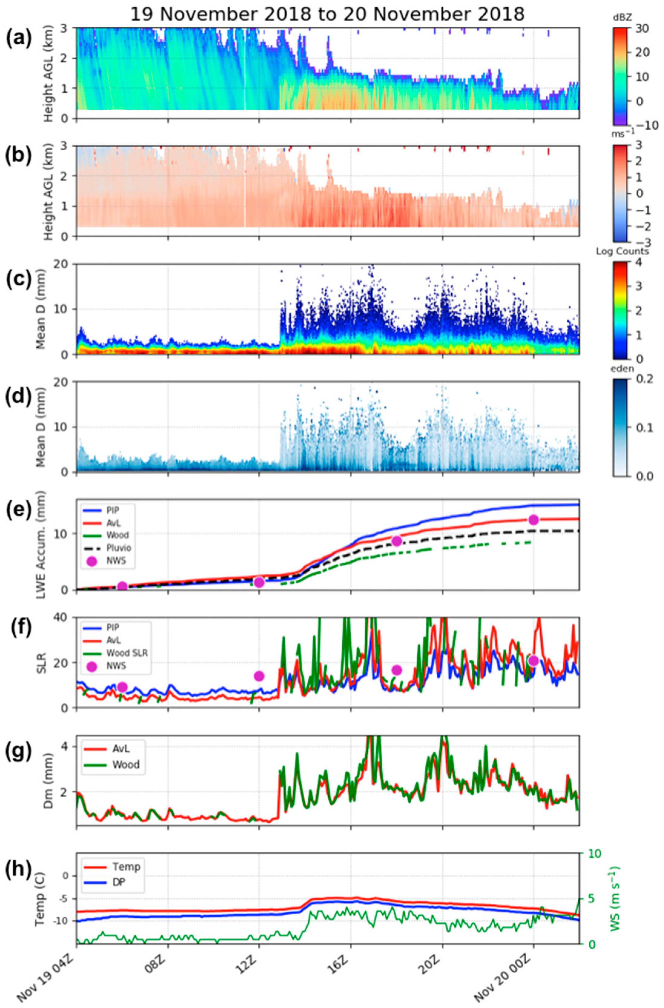
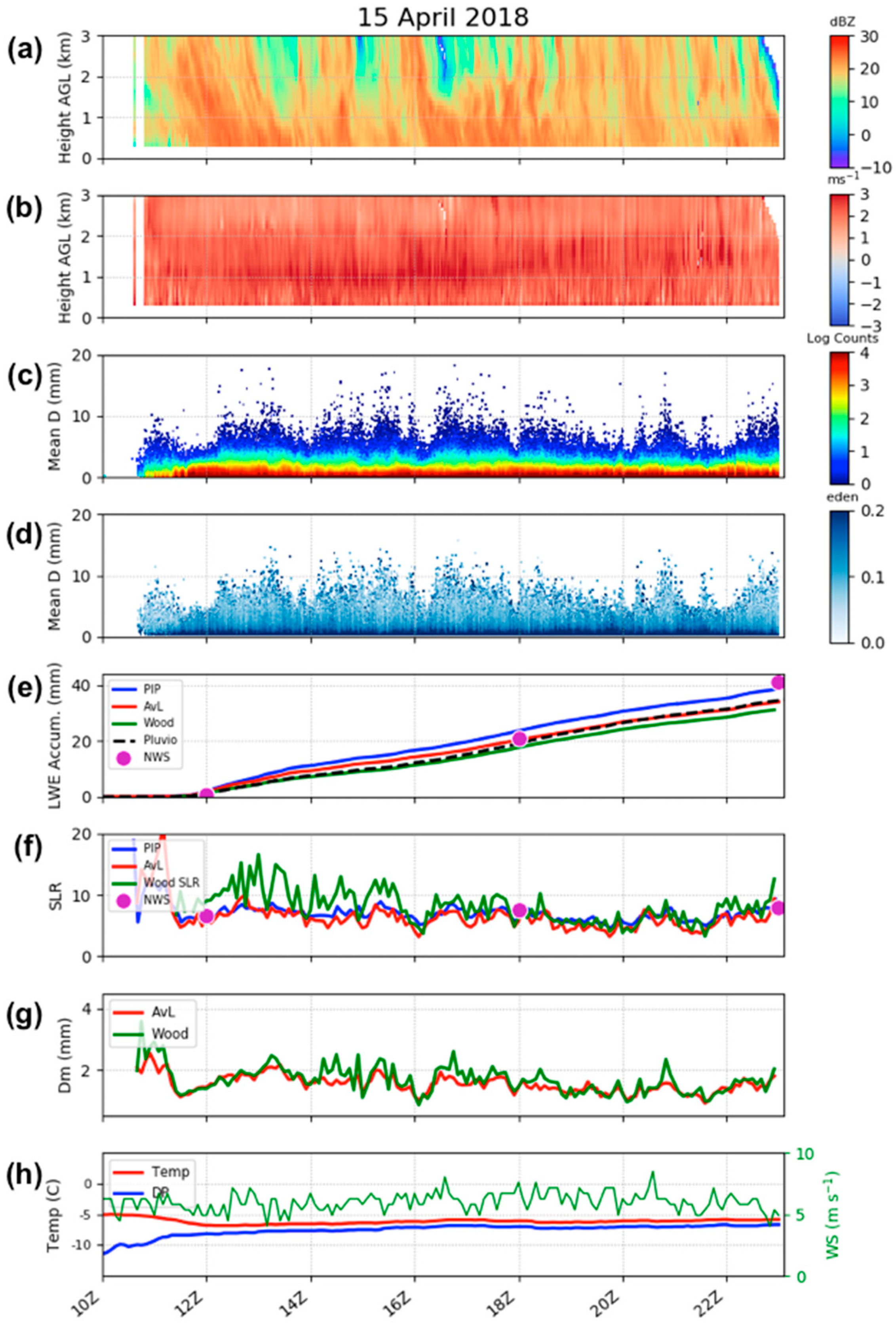
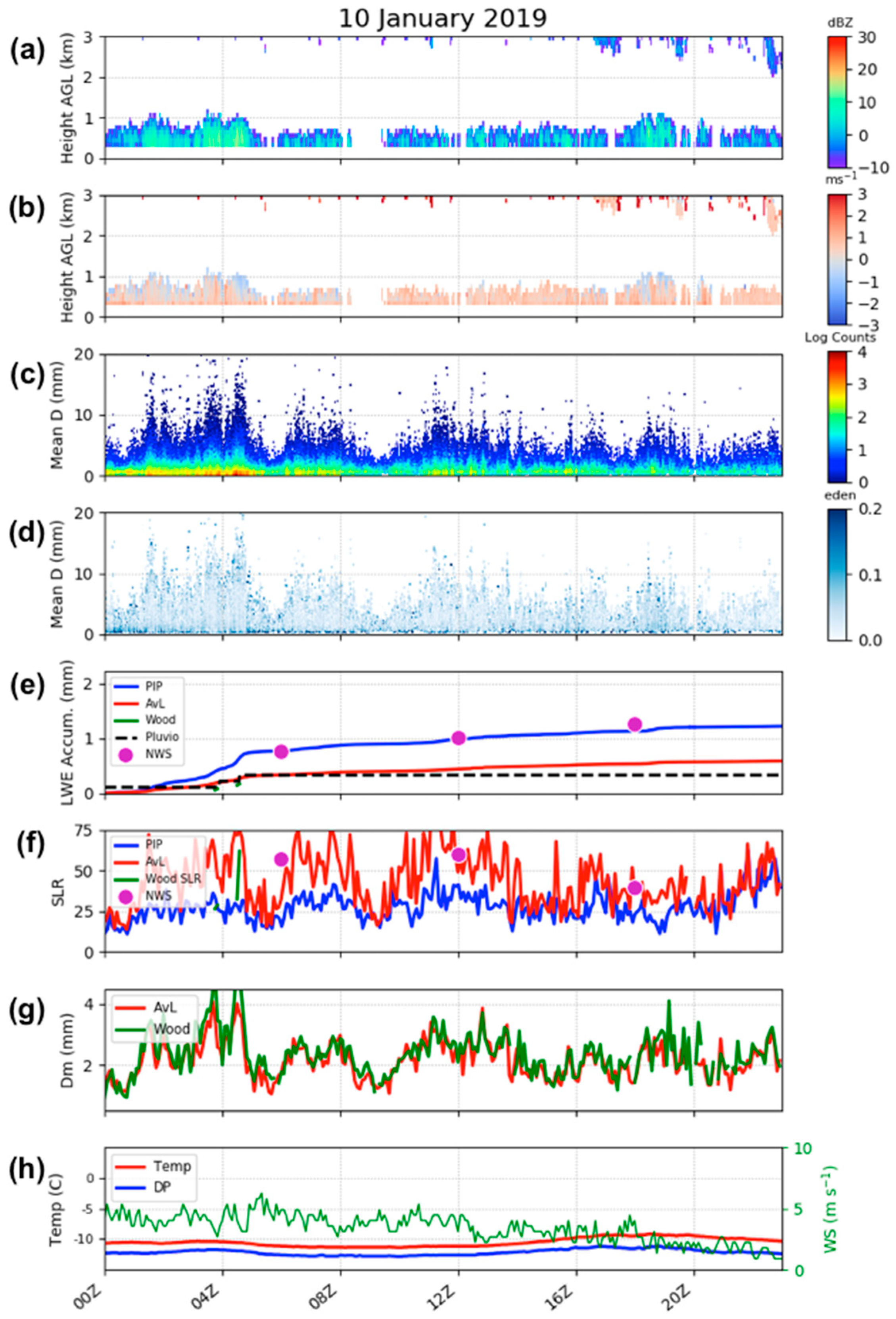
3.1. Low and High SLR Snow Event Characteristics

The low SLR snow events are shown in

Table 1. This is a table of the 11 low SLR snow events used in this work. Listed are the start and end times used for the analyses, as well as mean values of snow-to-liquid ratio (SLR), snow rate (here abbreviated as SR), wind speed (here abbreviated as WS), and temperature for the duration of each event.

Start (Date/Time)	End (Date/Time)	Mean SLR NWS	Mean SR PIP (mm h−1)	Mean WS (m s−1)	Mean Temp (°C)
11 November 2017 0600 UTC	11 November 2017 1200 UTC	12.14	0.899	3.33	−5.25
11 December 2017 1300 UTC	11 December 2017 1900 UTC	15	0.095	3.28	−8.95
13 December 2017 1000 UTC	13 December 2017 1800 UTC	13	0.278	1.55	−11.49
4 January 2018 0000 UTC	6 January 2018 1600 UTC	15.03	0.137	3.42	−17.16
22 January 2018 1800 UTC	23 January 2018 0300 UTC	7.5	3.751	3.96	−3.53
3 February 2018 1800 UTC	4 February 2018 0400 UTC	12	0.316	1.83	−12.88
12 April 2018 0800 UTC	12 April 2018 1600 UTC	10.45	1.672	0.88	−0.46
15 April 2018 1000 UTC	15 April 2018 2300 UTC	7.34	3.134	6.00	−6.41
2 December 2018 0600 UTC	3 December 2018 0300 UTC	9.11	2.455	4.73	−1.74
7 January 2019 0700 UTC	7 January 2019 2300 UTC	12.65	1.035	3.47	−2.22
20 January 2019 0600 UTC	21 January 2019 0600 UTC	14.89	0.274	2.87	−16.89

. These snow events have mean SLR values ranging from approximately 7.5:1 (extremely wet, dense snow) to 15:1 (commonly specified relationship for synoptically forced snowfall [50,51]). The mean PIP-derived snow rates vary widely from 0.095 to 3.75 mm h⁻¹. The observed event mean surface temperatures also have a large spread, ranging from −17 to −0.5 °C. There is a tendency for the warmer low SLR events (those with mean temperatures closer to 0 °C) to have higher mean snow rates. Generally speaking, the majority of these low SLR snow events are produced by synoptically forced, deep precipitation (figures not shown). However, two of the low SLR events would be categorized as shallow LeS: 4 January through 6 January 2018 and 20 January through 21 January 2019. Both of these low SLR LeS events have extremely cold temperatures (event means of −17 °C), which likely indicates that boundary layer temperatures were colder than the dendritic growth zone (DGZ) and would not be an environment conducive to large particle growth [52]. This is consistent with the characteristics of a secondary mode of LeS snow identified at MQT in previous work [19,20].

Characteristics of the high SLR snow events are shown in

Table 2. This is a table of the eight high SLR snow events used in this work. Organization follows that of Table 1.

Start (Date/Time)	End (Date/Time)	Mean SLR NWS	Mean SR PIP (mm h−1)	Mean WS (m s−1)	Mean Temp (°C)
14 December 2017 0000 UTC	14 December 2017 0800 UTC	32.75	0.259	2.59	−10.21
15 January 2018 2200 UTC	16 January 2018 2000 UTC	36.39	0.351	1.00	−9.76
28 January 2018 0800 UTC	28 January 2018 2300 UTC	70	0.054	2.48	−8.86
6 March 2018 1800 UTC	7 March 2018 2300 UTC	27.58	0.511	3.24	−7.26
13 March 2018 0400 UTC	7 March 2018 2300 UTC	30.33	0.132	3.94	−7.78
17 November 2018 0000 UTC	17 November 2018 2100 UTC	29.62	0.148	3.14	−6.04
25 November 2018 1200 UTC	26 November 2018 2000 UTC	30	0.079	3.49	−5.43
10 January 2019 0000 UTC	10 January 2019 2300 UTC	59	0.053	3.39	−10.50

. The high SLR snow events have mean SLRs from 28:1 (lower density snowfall) to greater than 50:1 (very low density), which are consistent with SLRs seen in previous studies of LeS [20,53,54]. Originally, we identified two additional ultralow density snow cases (SLR > 80:1); however, the Pluvio did not record any data during these events, which makes it difficult for the von Lerber and Wood methods to accurately retrieve mass. The mean PIP-derived snow rates are much lower than the low SLR events and a narrower range of values, from 0.079 to 0.511 mm h⁻¹. The event mean surface temperatures ranged from −10 to −5 °C, again a much smaller distribution than that of the low SLR snow events. All of the high SLR events were a product of surface and air interactions, namely LeS, orographic forcing, or both, as supported by the precipitation radar profiles (figures not shown).

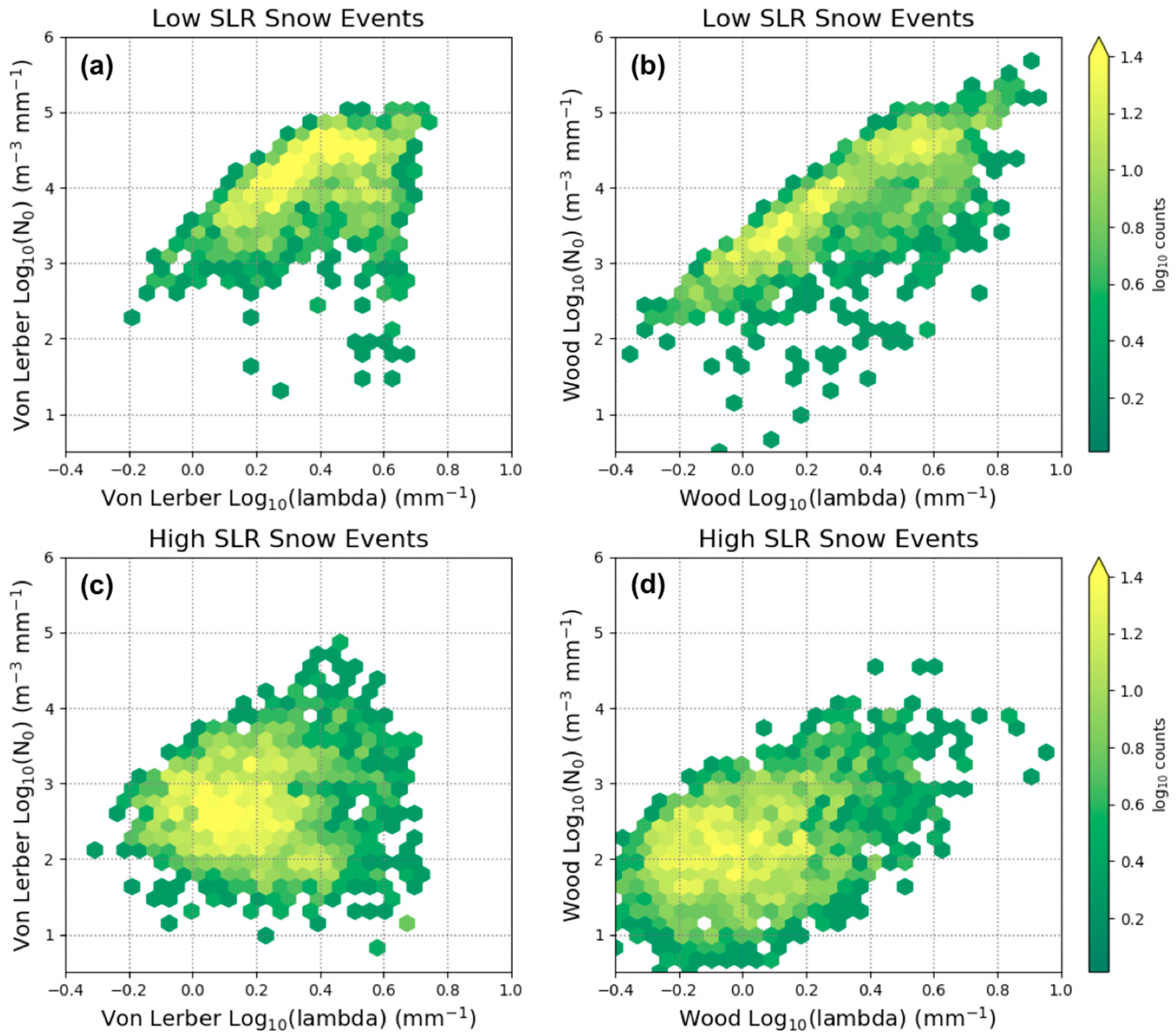
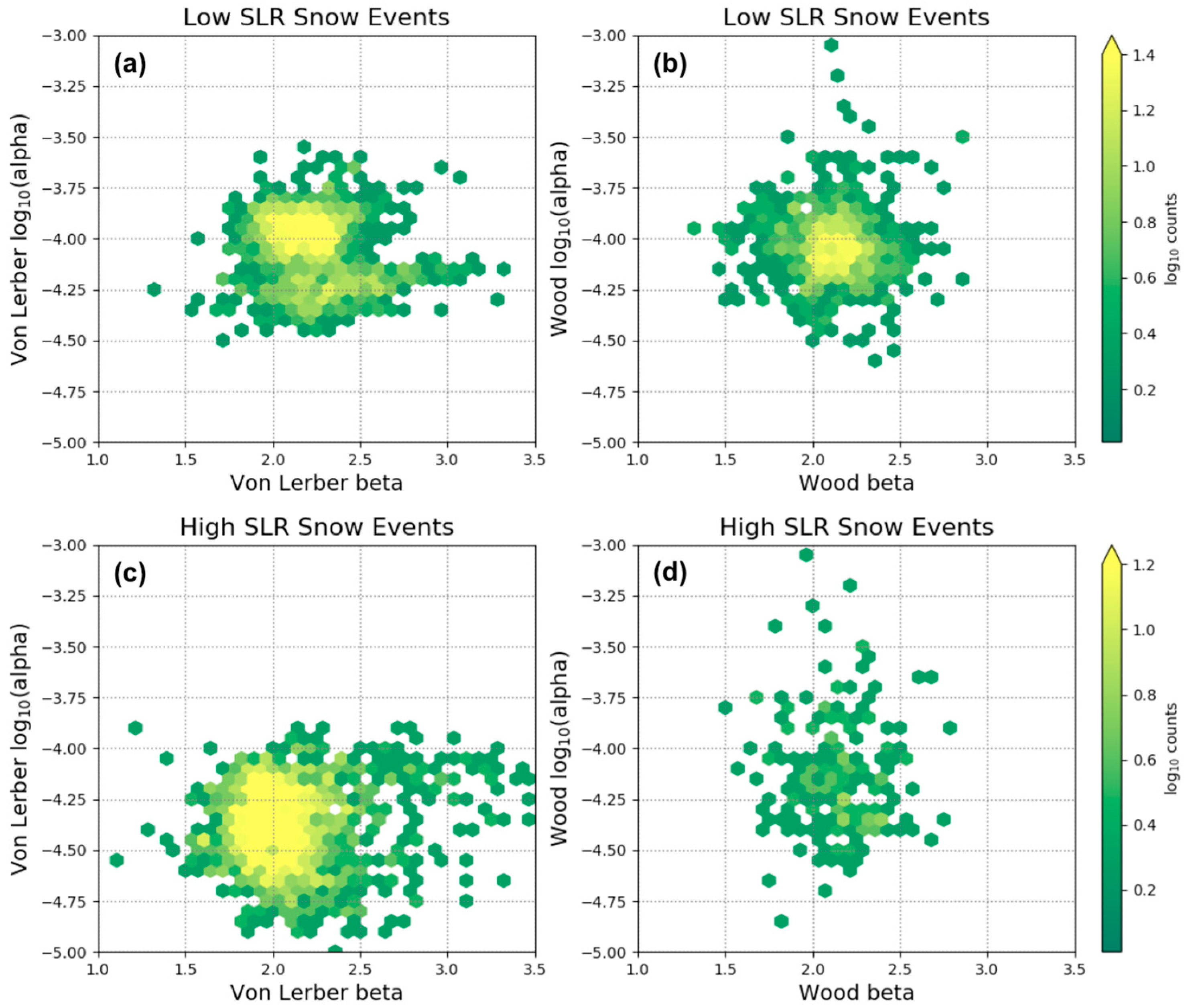
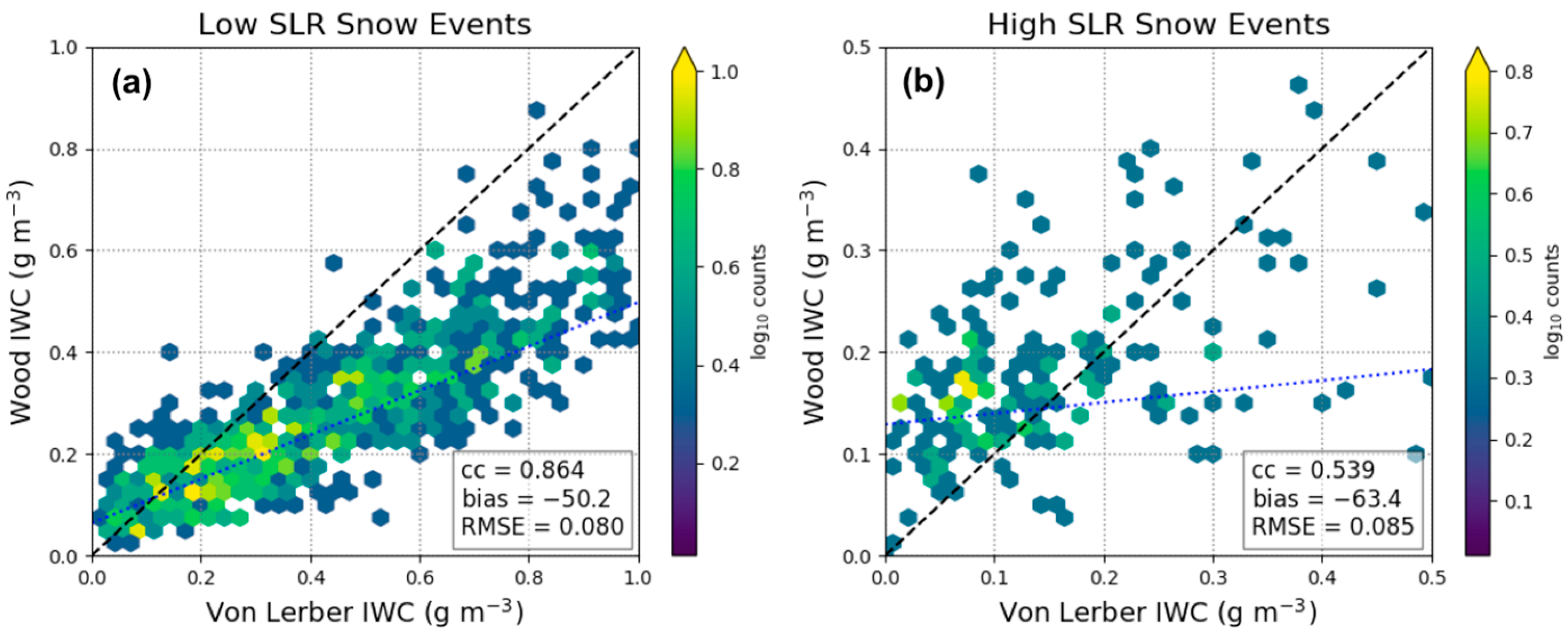
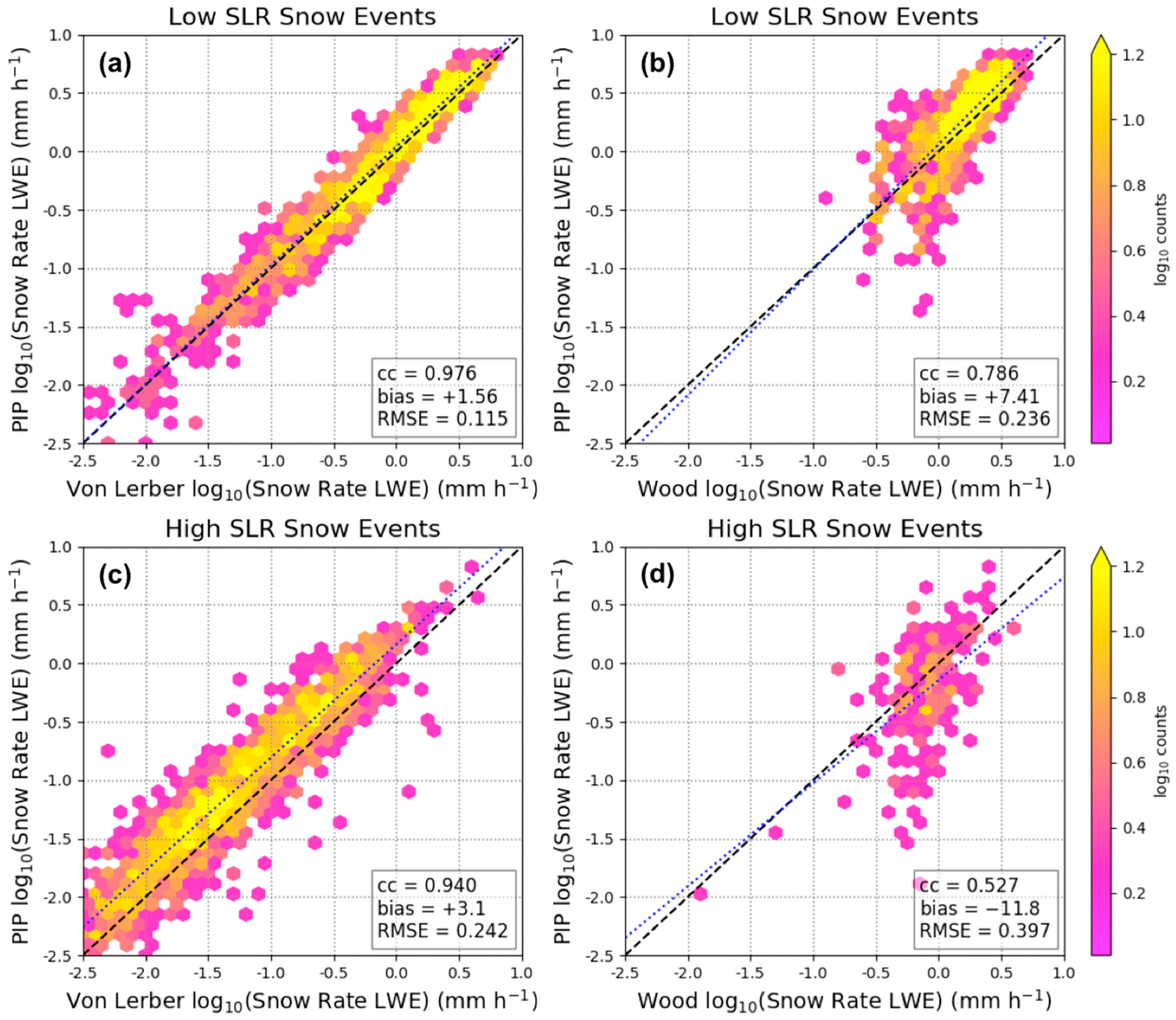
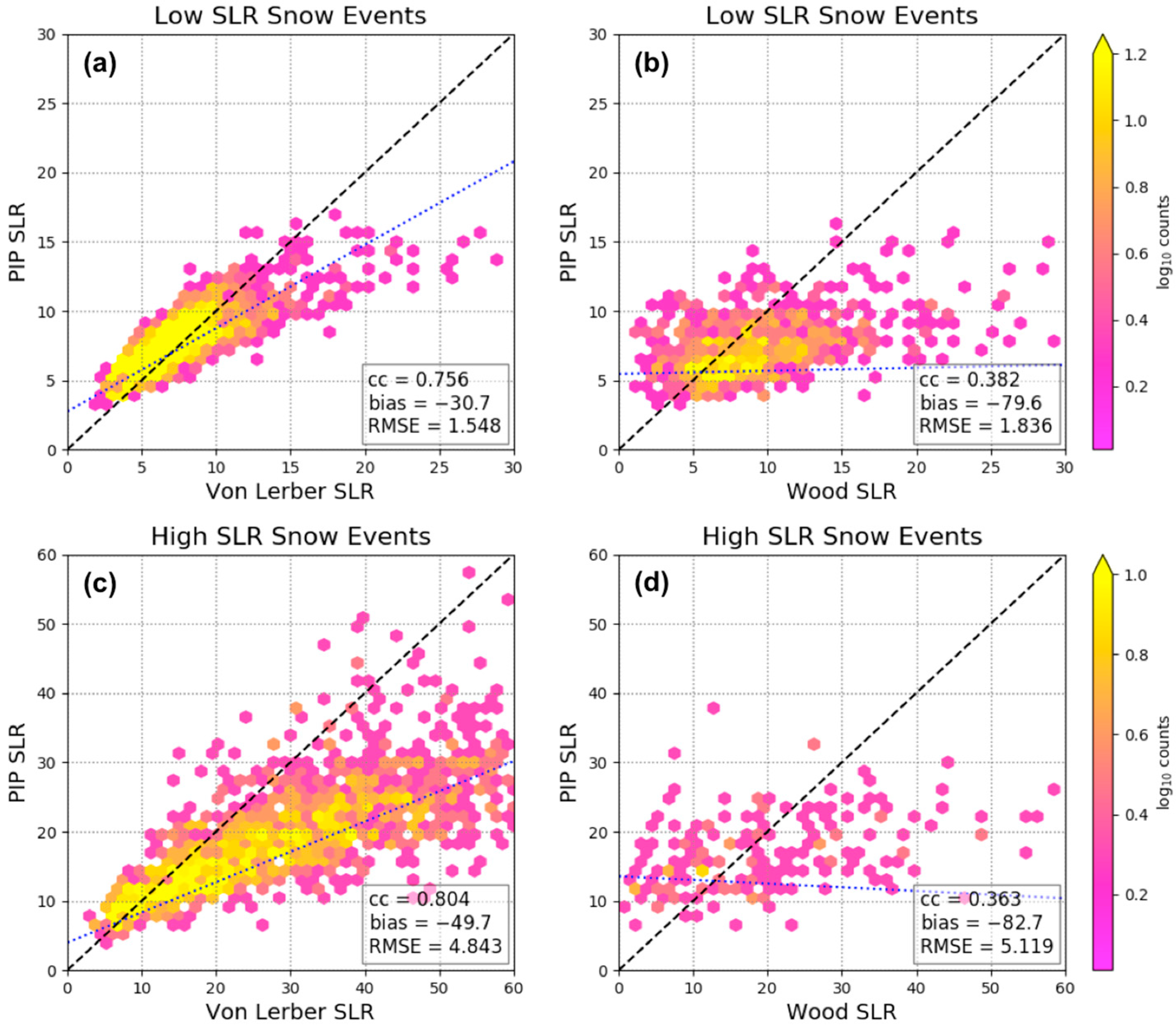
3.2. Snow Microphysical Characteristics

The PIP produces end-user products such as PSDs and size-resolved particle fall speeds, which illustrate microphysical characteristics of the snow. Figure 2 shows the PIP-derived PSDs for the low and high SLR events presented as two-dimensional histograms (Figure 2a,c, respectively). The low SLR snow events have large particle concentrations (>10³ m⁻³ mm⁻¹) at small D_e (<1 mm), while the high SLR snow events demonstrate a broader range of PSDs with an order of magnitude fewer small particles (most values <10³ m⁻³ mm⁻¹). These PSD results are consistent with prior studies of snowfall regimes [19]. The composite fall speed distributions also indicate differences between the low and high SLR events (Figure 2b,d, respectively). The low SLR snow composite implies generally higher fall speeds as a function of D_e compared to the high SLR snow composite, which has a flatter relationship and smaller particle fall speeds (<1 m s⁻¹). The mean fall speeds for the low SLR snow events are 30–45% larger than those for the high SLR snow events as a function of D_e for those D_e values <5 mm.

We also can examine the microphysical characteristics of the low and high SLR cases through differences between the shape of the size distributions for each category. Previous studies have applied the following inverse exponential relation to measured snow particle concentrations:

$$N\left(D_e\right)=N_0 \exp \left(-\mathsf{\Lambda } D_e\right)$$

(9)

where $N\left(D_e\right)$ is the particle concentration per particle size, D_e. N₀ and Λ are the PSD intercept and the slope parameter, respectively [19,55,56,57,58]. Both the von Lerber and Wood retrieval methods applied the relation in Equation (9) to 5 min intervals of the PIP data and each obtained N₀ and Λ for the low and high SLR events. There are differences in the resulting N₀ and Λ derived by the von Lerber and Wood methods due to differences in fitting methods and preprocessing of the PIP PSD data (see Section 2.2.2 and Section 2.2.3 for details).

Figure 3 illustrates composites of the derived von Lerber and Wood N₀ and Λ for the low SLR events (Figure 3a,b, respectively) and the high SLR events (Figure 3c,d, respectively). In general, the low SLR composites from the two methods show similar ranges, with N₀ ranging from 10² to 10⁵ m⁻³ mm⁻¹ and Λ values of 0.5 to 6.5 mm⁻¹ in a seemingly linear structure (see Figure 3a,b). The von Lerber shows fewer small values of both N₀ and Λ, which could be due to preprocessing that applies the threshold for total concentration and removes single occurring particle counts prior to the fitting routine (see Section 2.2.2). In both the von Lerber and Wood outputs, the high SLR events N₀ and Λ values are much smaller than that for the low SLR events, with N₀ ranging from 10 to 10⁴ m⁻³ mm⁻¹ and Λ ranging from 0.4 to 1.6 mm⁻¹, and no apparent relationship between the intercept and slope parameter. These results clearly show there are different shapes to the PSDs as a function of events that are low versus high SLR, which align with the results illustrated in Figure 2a,c. The median von Lerber values of both N₀ and Λ are 66% smaller for the high versus the low SLR snow events, while the median Wood value of N₀ is 58% smaller and Λ is 49% smaller for the high versus low SLR snow events. The N₀ and Λ results from the low SLR composite imply that these snowfall events have narrow PSDs with large amounts of small particles, similar to what has been observed for previous synoptically forced snow [19,55,58,59,60]. While the high SLR composite indicates the opposite: that these snow events tend to have broad PSDs with an order of magnitude fewer small particles and a tendency towards containing more large particles. The N₀ and Λ are similar to values seen in previous studies of LeS [19,56,61].

Additionally, we examined and compared the retrieved values of mass-weighted mean diameter for each SLR snow regime and the von Lerber and Wood methodologies. Mass-weighted mean diameter (D_m) is:

$$D_m=\frac{{\int }_{D_{min}}^{D_{max}}m\left(D_e\right)N\left(D_e\right)D_{e}dD}{{\int }_{D_{min}}^{D_{max}}m\left(D_e\right)N\left(D_e\right)dD}$$

(10)

There is good agreement (correlation coefficients (cc) of 0.945 and 0.883) between the von Lerber and Wood-derived values for D_m (see Figure 4). The high SLR event composite of D_m indicates a larger spread between the von Lerber and Wood values versus the low SLR, with the Wood D_m values generally higher for both categories (biases of +13.7% and +10.1%, respectively). In the low SLR event composite, both methods indicate that the majority of D_m values are smaller than 2 mm. However, in the case of the high SLR events, the range of values of D_m is much larger, extending from 1 to 4 mm, with a concentration towards larger values of D_m mostly between 1.5 and 3 mm. The median von Lerber value of D_m is 51% larger and the median Wood value of D_m is 56% larger for the high versus the low SLR snow events. The GPM Dual Precipitation Radar (DPR) algorithm has prescribed relationships for precipitation and D_m for stratiform and convective rainfall [21,62], and it is important to also examine these relationships for snowfall. Figure 4 illustrates that there are clear D_m differences for the low versus high SLR snowfall events. The SLR event types occur under different environmental conditions that should be therefore an additional factor that is considered when examining precipitation and D_m relations.

In addition, we investigated the output of the mass parameters, α and β, described in Equation (2), from the von Lerber retrieval (Figure 5a,c) and the Wood retrieval (Figure 5b,d). Note that the Wood retrieval outputs are fewer due to Pluvio limitations and filtering detailed in Section 2.2.3. (especially true for the high SLR cases). The low SLR events have scaling factor values, α, slightly larger than 10⁻⁴ and exponent, β, between 2 and 2.5 as produced by the von Lerber retrieval, while the Wood retrieval has a lower range of α (between 10^−4.25 and 10⁻⁴) and similar β (2–2.5). The von Lerber high SLR event composite shows much lower values for α (between 10^−4.75 and 10⁻⁴) and β (between 1.75 and 2.25). Though there are few points, the Wood retrieval also indicates lower α values, whereas the β range is similar to the low SLR output. Similar to the N₀ and Λ comparisons, we see that the low and high SLR snow event composite relations for α and β exhibit a clear separation, as illustrated in the von Lerber retrievals (Figure 5a,c). The values of both α and β are larger for the snow particles observed by the PIP during the low SLR events, which indicates that the mass increases faster as the area-equivalent diameter of the particle increases compared to the high SLR particles. The median of the von Lerber α values for the low SLR snow events is twice that of the high SLR, while the medians of the von Lerber β values are approximately the same for the low and high SLR (difference of 6%). The differences seen between the low versus high SLR events imply that snowfall retrieval algorithms, which rely on a priori assumptions of α and β either explicitly [48] or implicitly (e.g., Kulie and Bennartz [63], Liu [4], and Table 1, Braham et al. [64]), might benefit by adjusting to variations in snow type.

Finally, we compare the ice water content (IWC) retrieved by both the von Lerber and the Wood methods, for the low and high SLR snow events (see Figure 6a,b, respectively). Figure 6a evaluates the respective retrieved IWC values for the low SLR events. Though the IWC retrieved values are correlated (cc of 0.864) for the low SLR snow events, the Wood retrieval calculates much smaller IWC values versus the von Lerber retrieval, with a bias of –50%, and spread of 0.08 g m⁻³ as determined by the Root Mean Square Error (RMSE). In general, low SLR snow events produce more IWC values below 0.6 g m⁻³ for the von Lerber and 0.4 g m⁻³ for the Wood retrievals, respectively. The high SLR event composite has far fewer values to compare and there is a wide spread in the retrieval comparison and reduced correlation (cc of 0.539). There is an indication that the Wood output retrieves larger values of IWC matched to that of the von Lerber output; however, with so few points we can only suggest this is a possibility. There is evidence that the low SLR events produce more integrated mass as the median von-Lerber-retrieved value of IWC is more than an order of magnitude larger for the low SLR versus the high SLR snow events.

In general, the low SLR snow events have an order of magnitude more small particles and 30 to 45% higher fall speeds than the high SLR snow events. Both the von Lerber and Wood-derived values of N₀ and Λ are smaller (66% and ~50%, respectively) for the high versus low SLR snow events, which is consistent with findings from Pettersen et al. [19]. The D_m values for the high SLR snow events are larger for von Lerber (51%) and Wood (56%) versus the low SLR events. The median von-Lerber-retrieved value of α was two times larger for the low SLR versus the high SLR snow events, while the β values were approximately the same. The von-Lerber-retrieved IWC was more than an order of magnitude larger for the low versus the high SLR snow events. In terms of comparisons between the retrievals, the Wood D_m values were between 10% and 14% larger than the von Lerber D_m values, regardless of snow event type, and the D_m values for the retrievals were highly correlated (cc values of 0.88 and 0.95). The Wood-retrieved values of IWC were biased 50% lower than the von Lerber IWC values for the low SLR snow events; however, the retrieved values were highly correlated between the retrieval methods (cc of 0.86).

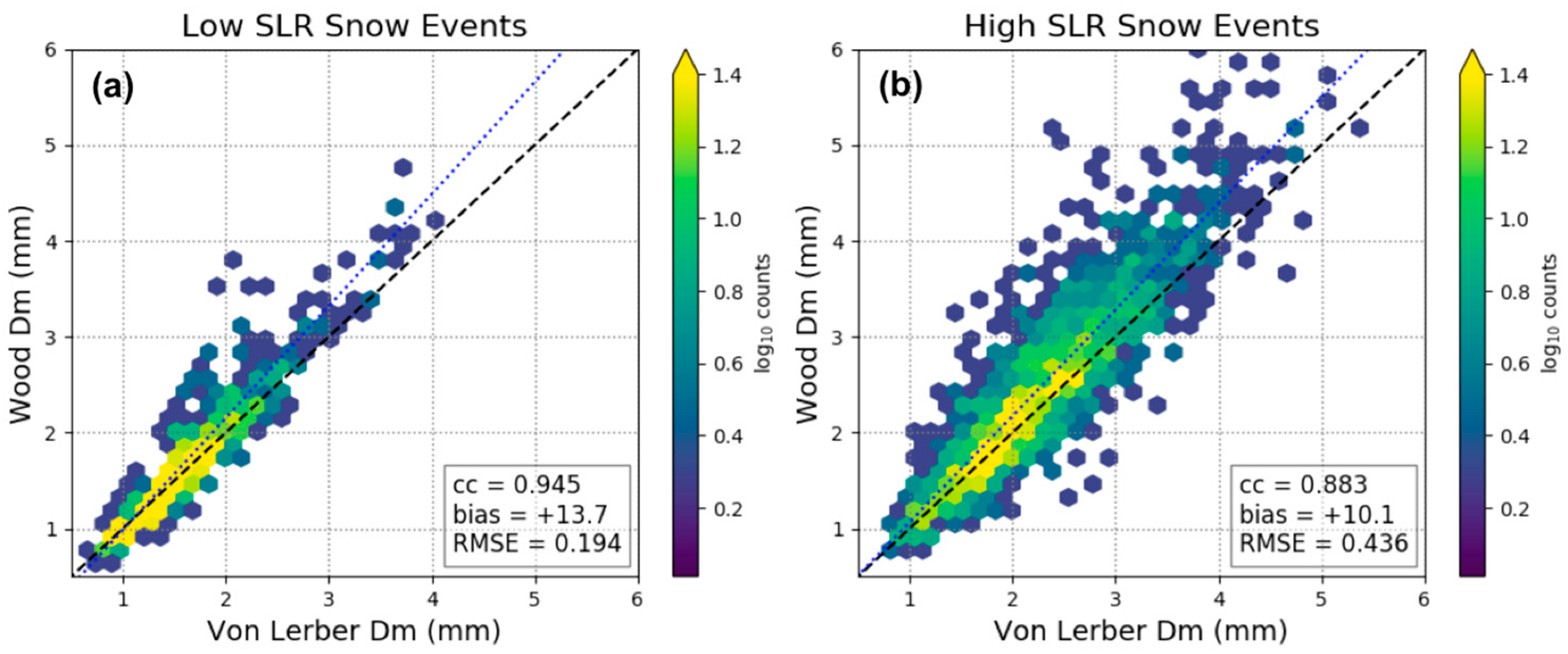
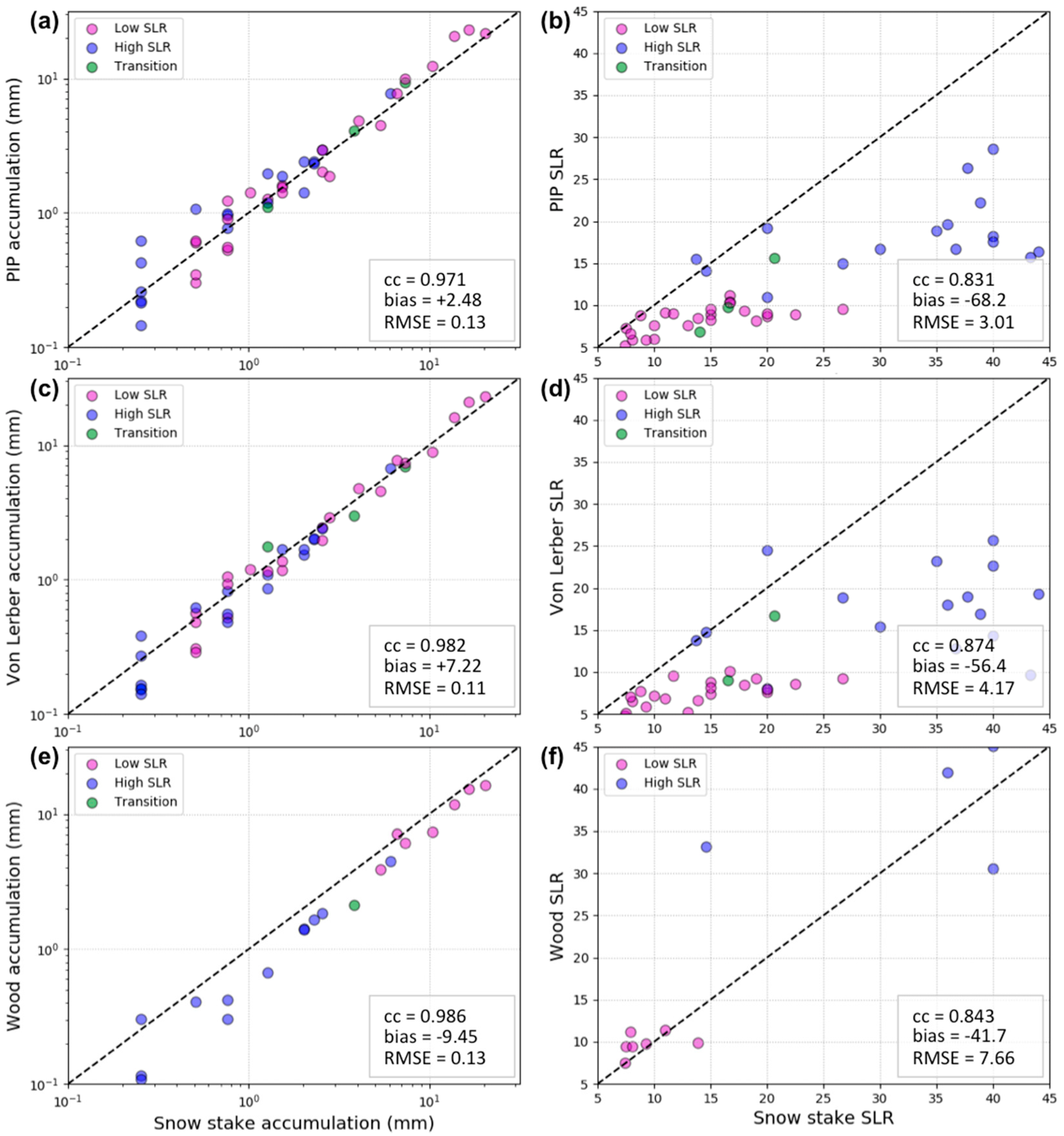
3.3. Bulk Snowfall Characteristics

We have shown that using snow observations from the PIP the von Lerber and Wood-retrieved microphysical characteristics compared well and showed consistent differences between the low and high SLR events. Additionally, the values of α, β, and mass were physically reasonable and again illustrated distinct relationships for the low and high SLR snow events. Here, we examine and intercompare the bulk characteristics of the low and high SLR snow events from the PIP higher-order-derived data products and the von Lerber and Wood retrievals. The intercomparison focuses on the produced values of snow rate and $\overline{{\rho }_e}$.

Figure 7 highlights comparisons of the PIP-produced LWE precipitation rates (on the y-axes) with those from the von Lerber (Figure 7a,c) and Wood (Figure 7b,d) methods for the low (Figure 7a,b) and high (Figure 7c,d) SLR snow events. For the low SLR event composites, we see LWE precipitation rates up to 6 mm h⁻¹ with a very high correlation between the PIP-derived snow rates and the output from von Lerber (cc of 0.976), while less correlated with the snow rates retrieved from Wood (cc of 0.786). In general, the LWE precipitation rates are less than 2 mm h⁻¹, but there are indications of repeated instances of higher rate values. The PIP LWE precipitation rates tend to be in good agreement with those of von Lerber, a bias of +1.56%, but biased high with respect to Wood (+7.41%) for the low SLR snow events. For high SLR snow events, the PIP and von Lerber retrievals compare well (cc of 0.940), with a linear relationship as LWE precipitation rates increase. There is again good agreement between the produced snow rates, with the PIP is biased slightly high (+3.1%) compared to the von Lerber values. Many of the high SLR snow event samples provided physically inconsistent inputs for the Wood method and were so excluded (see Section 2.2.3), so it is difficult to compare. However, we can compare the differences between the low and high SLR snow events by examining the PIP and von Lerber produced values of snow rate. Though the RMSE between the PIP and von Lerber values of snow rate is 0.115 mm h⁻¹ for the low SLR and 0.242 mm h⁻¹ for the high SLR snow events, the median values for the event regimes agree very well, with a 4% difference for the low SLR and a 9% difference for the high SLR snow events. Unsurprisingly, the low SLR snow events have much larger LWE precipitation rates, with median rates more than 20 times higher compared to the high SLR snow events for both the PIP and von Lerber outputs.

We also assess the respective values of $\overline{{\rho }_e}$ (g cm⁻³) for the low and high SLR snow events (see Figure 8). As discussed in Section 2.2.1, the SLR output from the three methods is roughly the inverse of the ratio $\overline{{\rho }_e}$ to the density of water (1 g cm⁻³); however, it is important to note that this conversion does not account for compaction effects. Here, we compare the $\overline{{\rho }_e}$ values by inverting them to produce bulk SLR values for each time step. The low and high SLR events were defined using SLR observations from the NWS MQT snow field, and therefore we expect the comparisons in Figure 8 to have different ranges of PIP, von Lerber, and Wood produced SLRs as a function of event category, regardless of method. We see for the low SLR snow event composites (Figure 8a,b) that the vast majority of SLR values are less than 10:1 for the PIP, von Lerber, and Wood retrievals. The SLR output from the PIP and the von Lerber retrievals have a correlation of 0.756. There is a shift for SLR of >15 where von Lerber reports larger values compared to the PIP, which results in the PIP values biased 30% lower than output from von Lerber. However, the median values of the PIP and von-Lerber-derived SLR are within 6%. The low SLR composite for the PIP and Wood-derived SLR have a low correlation (cc of 0.382), and an inclination for the PIP SLR to be much lower than that of the Wood output (bias of –79.6%). The high SLR event composite between the PIP and von Lerber SLRs (Figure 8c) show a similar correlation to the low SLR composite (cc of 0.804); however, with more variability (RMSE of 4.843), and a low bias of almost 50%. Additionally, the median PIP-produced SLR value is 60% smaller than that of von Lerber for the high SLR snow events. There are too few values of the Wood method for the high SLR snow events to conclude similarities or differences with the PIP output (Figure 8d).

The PIP and von Lerber low (Figure 8a) and high (Figure 8c) SLR event composites illustrate that the majority of the prescribed low SLR snow event values are <10:1, whereas the high SLR snow event SLRs range from 8:1 to 30:1, with some of the von Lerber values extending to 60:1 (note different x and y limits). Additionally, the median PIP value for the high SLR snow events is twice that of the low SLR snow events, while the corresponding von Lerber median values are 3.6 times larger. The range of SLRs values for the high SLR snow events is much larger than that of the low SLR snow events.

Though much of the focus of this work is an intercomparison of the bulk snow products from the PIP higher-order products and the von Lerber and Wood retrievals, we additionally wanted to assess each method against an established means of acquiring accumulation to produce uncertainty estimates. Here, we examine the six-hourly accumulation and SLR values from NWS MQT snow field measurements for all the presented snow events against corresponding intervals of accumulation. These accumulation comparisons are presented in Figure 9 with the NWS MQT snow accumulation observations on the respective x-axes (left panels). There is a high correlation between the six-hourly accumulations from the respective methods and the snow field observations, with PIP cc of 0.971, von Lerber cc of 0.982, and Wood cc of 0.986. The PIP-produced and von-Lerber-retrieved accumulations show excellent agreement with the snow field observations, where each is biased slightly high at +2.48% and +7.22%, respectively, The Wood-retrieved accumulations also agree very well; however, are biased slightly lower than the snow field at −9.45%. The accumulations for all three methods RMSE range from 0.11 to 0.13 mm per 6 h interval. The PIP (Figure 9a) and von-Lerber-derived (Figure 9c) accumulation comparisons have 46 and 44 6 h interval matches, respectively, while the Wood accumulation only had 22 6 h accumulation comparison points due to the Pluvio filtering method (see Section 2.2.3).

Additionally, we compare the six-hourly observations of SLR from the NWS MQT snow field (x-axes in Figure 9b,d,f) and the median SLR produced by each method. The PIP, von Lerber, and Wood median SLR tended to be lower than that measured by the snow field with biases of −68.2%, −56.4%, and −41.7%, respectively; however, all are well correlated (cc of 0.831, 0.874, and 0.843, respectively). The high SLR snow event median SLRs (purple circles) tend to have much more spread, which is unsurprising given the large variability in LeS and orographic snow events. There is less agreement between the snow field and the Wood SLR values; however, there are also fewer points (22) to compare. In general, the Wood median SLRs for the low SLR events agree better with the snow field than the retrieved values for the high SLR events. Additionally, the Wood median SLRs for the same time periods as the PIP and von Lerber median SLRs correspond well for the low SLR event samples; however, they do not for the high SLR events (figure not shown).

The results imply fundamental differences in the bulk snow characteristics between the low and high SLR snow regimes. The low SLR snow events produced much larger LWE snow rates, as both the PIP and von Lerber indicated 20 times higher values compared to the high SLR snow events. The differences in snow rates seen between the low SLR (primarily synoptically forced snow events) and high SLR (LeS and orographically forced snow events) are consistent with differences observed in previous studies [19,20,37]. Unsurprisingly, the PIP and von Lerber determined median values of SLR were 2 and 3.6 times larger, respectively, for the high versus the low SLR snow events. The high SLR snow events tended to have a much larger spread of values of PIP and von Lerber determined SLR, which could be due to the large variability inherent in surface-based processes by different forcing mechanisms (LeS versus orographic) and boundary-layer conditions [19,20]. In terms of intercomparisons of snow rates, there was excellent agreement between the three methods for the low SLR snow events, with the PIP values biased +1.58% compared to the von Lerber retrieval and +7.41% compared to the Wood retrieval. For the high SLR snow events, there was again excellent agreement with the PIP values biased +3.1% compared to the von-Lerber-retrieved values. When compared to the NWS snow field measurements of six-hourly accumulation, the retrievals all showed consistent results: The PIP accumulations were only biased +2.48% higher with an RMSE of 0.13 mm per 6 h time interval; the von Lerber retrievals of accumulation had a high bias of +7.22% and RMSE of 0.11 mm; and the Wood retrievals were biased −9.45% lower than the snow field accumulation with an RMSE of 0.13 mm per 6 h period. It is important to note that the PIP-produced accumulations agreed best with the NWS snow field and, unlike the Wood and von Lerber retrievals, do not use any information from the snow field to calculate the event accumulations. Although the scatter shown in Figure 7 suggests the fractional uncertainties in high-time resolution snow rates have larger spread (especially when compared to the Wood retrievals), Figure 9 indicates that 6 h PIP estimates of accumulation or mean snowfall rate appear to have uncertainties smaller than 5%.

3.4. Detailed Example of a Snow Transition Event

Throughout this analysis, we have presented the output from the PIP, von Lerber, and Wood methods using a composited approach that highlights the differences between the low and high SLR snow events, while simultaneously showing that the PIP higher-order-derived products accurately represent the bulk snow conditions. We additionally want to emphasize the utility of these methods to examine the snow characteristics as a function of individual events. In this subsection, we present a snow event that transitions from low to high SLR snowfall under changing environmental conditions. Detailed examples of low and high SLR events can be found in Appendix B (Figure A1 and Figure A2, respectively). The event is presented with ancillary data from the profiling radar (MRR), the Pluvio, and snow field accumulations, the surface meteorological conditions, and the output from the von Lerber and Wood retrievals to give further context and support to the PIP-derived data products.

We examine an event that started as synoptically forced snow and transitioned to lake-enhanced snowfall [20,65] from 19 November (0400 UTC) to 20 November 2018 (0200 UTC), shown in Figure 10. During the beginning of the event (prior to 1300 UTC), the MRR profile indicates a deep precipitation column of light snowfall (reflectivities <10 dBZ; Figure 10a) and comparatively slow fall speeds (<1 m s⁻¹; Figure 10b). We also see that the PIP PSDs are very narrow during this time period with particles smaller than 5 mm D_e (Figure 10c). Additionally, the PIP ${\rho }_e$ distribution values are greater than 0.1 g cm³ (10:1 SLR) during the early part of the snow event (Figure 10d). At 1300 UTC, we see an abrupt change in the observations with increasing reflectivity and Doppler velocity values with decreasing precipitation height (~1.5 km AGL). At this same time, the PIP PSDs respond with an immediate broadening (particles ranging up to 15 mm D_e), while still maintaining a high concentration of small particles (>10⁴ particles smaller than 1 mm D_e). We also see that the ${\rho }_e$ distribution shifts to lower values, generally less than 0.1 g cm⁻³ (Figure 10d). The accumulation (Figure 10e) is gradual during the low SLR period of the snow event, but the snow rate increases directly following the transition at 1300 UTC, with ~9 mm accumulation in 6 h (in agreement with the von Lerber accumulation). Overall, the von Lerber total accumulation exactly matched the NWS MQT snow field, while the PIP recorded a relatively higher amount (120%) and the Wood retrieval much less (67%). Unsurprisingly, we see an instantaneous response from the values of SLR and D_m at 1300 UTC as well (Figure 10f,g, respectively), and both increase rapidly, with SLR values from 10:1 to greater than 20:1 and average D_m growing from ~0.5 to more than 2 mm. During the transition period, winds shift to slightly higher speeds (Figure 10h) and more northerly direction.

4. Conclusions

The primary goal of this work was to define and demonstrate the quality and efficacy of the PIP higher-order products. The results detailed in this work confirm the ability of the PIP-derived products to quantify properties of LWE snow rate, ${\rho }_e$, and SLR. Specifically, through comparisons with established mass retrieval methods from von Lerber et al. [17] and Wood et al. [30], we have shown that the PIP produces physically consistent bulk snow characteristics and produces LWE snow rates that agree with these methods within 1.5 to 12% depending on snow type and retrieval. Additionally, the PIP-derived LWE accumulations over 6 h periods match the NWS MQT snow field measurements for both the low and high SLR events, suggesting that the PIP LWE snow rates are accurate for the examined snowfall. The PIP accumulations were within 2.48% of those for the NWS snow field observations and, unlike the von Lerber and Wood retrievals which made use of the snow stake field observations directly or indirectly, were produced with no ancillary information of precipitation rate or accumulation. The von Lerber and Wood-derived six-hourly accumulations also showed consistent results with the NWS MQT snow field measurements, agreeing within 10%. Furthermore, the results from this work indicate that the PIP is much better at detecting small accumulations of snow compared to the unfenced Pluvio gauge. The large number of samples for which the Pluvio detected no accumulations and the PIP (and MRR) indicated significant snowfall, particularly prevalent for the high SLR events, underscores this point. These results imply that the PIP is less impacted by wind and therefore has less or no undercatch. This may be due to the advantage that the PIP is able to sample in a large and unimpeded volume, where the Pluvio has only a small opening for which to receive falling particles. The PIP is therefore well suited to providing time series of snowfall rates and SLR at a high-time resolution, as is exhibited in the detailed analysis of specific snow events (see Figure 10, Figure A1, and Figure A2).

We also found that there are distinct microphysical and bulk characteristics for the low and high SLR snow events, as illustrated by the three retrieval methods. The PIP-produced PSDs, fall speeds, and relationships of N₀ and Λ were very different for the low versus high SLR and consistent with values found in previous studies of synoptically forced and lake-effect snowfall. In general, the D_m values for the high SLR snow events are larger and more variable than those for the low SLR snow events. Similar to the N₀ and Λ comparisons, we see that the low and high SLR snow event composite relations for α and β exhibit a clear separation, with lower values of both for the high SLR snow events. There were too few IWC values for the high SLR snow events to compare the von Lerber and Wood methods, but low SLR IWC values are generally larger. In general, the PIP LWE snow rates compared well to those produced by the retrieval methods for the high and low (von Lerber only) density events. The PIP and von-Lerber-retrieved values of SLR were consistent for both low and high SLR snow events, with the von Lerber method producing consistently larger values. Finally, accumulation comparisons between all three methods and the six-hourly snow field were excellent for both the low and high SLR snow events.

Future work will focus on a few key areas. First, to develop a means to produce real-time uncertainty estimates for the PIP LWE snow rate and ${\rho }_e$ products. Second, to enhance the current PIP ${\rho }_e$ parameterization. As outlined in Section 2.2.1, the PIP ${\rho }_e$ parameterization is currently constrained and tested by empirical observations from only three events with a limited range of SLRs. Further analysis of extreme high SLR, higher density (<10:1), and mixed-phase snow events, as well as those containing a majority of graupel and rimed particles will help to improve the ${\rho }_e$ parameterization. Third, continue to expand our understanding of the meteorological and environmental factors on the retrieved snow micro- and macrophysical characteristics. This work indicates that there are specific microphysical relations and bulk characteristics that are connected to the ambient environment, and further analysis could illuminate key snow processes.

The PIP has been used in several field campaigns and long-term deployments all over the world, and these data are available for continued examination of snow. The PIP observations and higher-order products serve as valuable constraints on microphysical assumptions in ground-based and spaceborne remotely sensed snowfall retrievals. Additionally, this work illustrates that the higher-order PIP-derived LWE snow rate and ${\rho }_e$ values are physically consistent and valid when compared to several retrieval methods and measurements. Furthermore, the PIP captures accumulation during snow conditions under which traditional precipitation gauges are unable, due to the unique open volume design. The PIP data and higher-order products are an invaluable resource to the snow and precipitation communities.

5. Data Availability

All data used in this study can be acquired from the NASA Global Hydrology Research Center data archive (https://ghrc.nsstc.nasa.gov/home/).

References

1. Klazura, G.E.; Imy, D.A. A description of the initial set of analysis products available from the NEXRAD WSR-88D system. Bull. Am. Meteorol. Soc. 1993, 74, 1293–1312. [Google Scholar] [CrossRef] [Green Version]
2. Stephens, G.L.; Vane, D.G.; Tanelli, S.; Im, E.; Durden, S.; Rokey, M.; Reinke, D.; Partain, P.; Mace, G.G.; Austin, R.; et al. CloudSat mission: Performance and early science after the first year of operation. J. Geophys. Res. Atmos. 2008, 113. [Google Scholar] [CrossRef]
3. Hou, A.Y.; Kakar, R.K.; Neeck, S.; Azarbarzin, A.A.; Kummerow, C.D.; Kojima, M.; Oki, R.; Nakamura, K.; Iguchi, T. The global precipitation measurement mission. Bull. Am. Meteorol. Soc. 2014, 95, 701–722. [Google Scholar] [CrossRef]
4. Liu, G. Deriving snow cloud characteristics from CloudSat observations. J. Geophys. Res. Atmos. 2008, 113. [Google Scholar] [CrossRef] [Green Version]
5. Kulie, M.S.; Bennartz, R.; Greenwald, T.J.; Chen, Y.; Weng, F. Uncertainties in microwave properties of frozen precipitation: Implications for remote sensing and data assimilation. J. Atmos. Sci. 2010, 67, 3471–3487. [Google Scholar] [CrossRef] [Green Version]
6. Skofronick-Jackson, G.M.; Johnson, B.T.; Munchak, S.J. Detection thresholds of falling snow from satellite-borne active and passive sensors. IEEE TGRS 2013, 51, 4177–4189. [Google Scholar] [CrossRef] [Green Version]
7. Wood, N.B.; L’Ecuyer, T.S.; Bliven, F.L.; Stephens, G.L. Characterization of video disdrometer uncertainties and impacts on estimates of snowfall rate and radar reflectivity. Atmos. Meas. Tech. 2013, 6, 3635–3648. [Google Scholar] [CrossRef] [Green Version]
8. Von Lerber, A.; Moisseev, D.; Marks, D.A.; Petersen, W.; Harri, A.M.; Chandrasekar, V. Validation of GMI Snowfall Observations by Using a Combination of Weather Radar and Surface Measurements. J. Appl. Meteorol. Climatol. 2018, 57, 797–820. [Google Scholar] [CrossRef]
9. Hiley, M.J.; Kulie, M.S.; Bennartz, R. Uncertainty analysis for CloudSat snowfall retrievals. J. Appl. Meteorol. Climatol. 2011, 50, 399–418. [Google Scholar] [CrossRef]
10. Kneifel, S.; Kulie, M.S.; Bennartz, R. A triple-frequency approach to retrieve microphysical snowfall parameters. J. Geophys. Res. 2011, 116, D11203. [Google Scholar] [CrossRef] [Green Version]
11. Johnson, B.T.; Petty, G.W.; Skofronick-Jackson, G. Microwave properties of ice-phase hydrometeors for radar and radiometers: Sensitivity to model assumptions. J. Appl. Meteorol. Climatol. 2012, 51, 2152–2171. [Google Scholar] [CrossRef] [Green Version]
12. Olson, W.S.; Tian, L.; Grecu, M.; Kuo, K.S.; Johnson, B.T.; Heymsfield, A.J.; Bansemer, A.; Heymsfield, G.M.; Wang, J.R.; Meneghini, R. The Microwave Radiative Properties of Falling Snow Derived from Nonspherical Ice Particle Models. Part II: Initial Testing Using Radar, Radiometer and In Situ Observations. J. Appl. Meteorol. Climatol. 2016, 55, 709–722. [Google Scholar] [CrossRef]
13. Wood, N.B.; L’Ecuyer, T.S.; Heymsfield, A.J.; Stephens, G.L. Microphysical constraints on millimeter-wavelength scattering properties of snow particles. J. Appl. Meteorol. Climatol. 2015, 54, 909–931. [Google Scholar] [CrossRef] [Green Version]
14. Tyynelä, J.; von Lerber, A. Validation of Microphysical Snow Models Using In Situ, Multifrequency, and Dual-Polarization Radar Measurements in Finland. J. Geophys. Res. Atmos. 2019, 124, 13273–13290. [Google Scholar] [CrossRef]
15. Tiira, J.; Moisseev, D.N.; von Lerber, A.; Ori, D.; Tokay, A.; Bliven, L.F.; Petersen, W. Ensemble mean density and its connection to other microphysical properties of falling snow as observed in Southern Finland. Atmos. Meas. Tech. 2016, 9. [Google Scholar] [CrossRef] [Green Version]
16. Newman, A.J.; Kucera, P.A.; Bliven, L.F. Presenting the snowflake video imager (SVI). J. Atmos. Ocean. Technol. 2009, 26, 167–179. [Google Scholar] [CrossRef]
17. von Lerber, A.; Moisseev, D.; Bliven, L.F.; Petersen, W.; Harri, A.M.; Chandrasekar, V. Microphysical properties of snow and their link to Ze–S relations during BAECC 2014. J. Appl. Meteorol. Climatol. 2017, 56, 1561–1582. [Google Scholar] [CrossRef]
18. Falconi, M.T.; Lerber, A.V.; Ori, D.; Marzano, F.S.; Moisseev, D. Snowfall retrieval at X, Ka and W bands: Consistency of backscattering and microphysical properties using BAECC ground-based measurements. Atmos. Meas. Tech. 2018, 11. [Google Scholar] [CrossRef] [Green Version]
19. Pettersen, C.; Kulie, M.S.; Bliven, L.F.; Merrelli, A.J.; Petersen, W.A.; Wagner, T.J.; Wolff, D.B.; Wood, N.B. A composite analysis of snowfall modes from four winter seasons in Marquette, Michigan. J. Appl. Meteorol. Climatol. 2020, 59, 103–124. [Google Scholar] [CrossRef]
20. Kulie, M. Upper Great Lakes Snowfall: Lessons Learned from a Multi-Sensor Snowfall Observatory; BAMS: Boston, MA, USA, submitted.
21. Chase, R.J.; Nesbitt, S.W.; McFarquhar, G.M. Evaluation of the microphysical assumptions within GPM-DPR using ground-based observations of rain and snow. Atmosphere 2020, 11, 619. [Google Scholar] [CrossRef]
22. Adhikari, A.; Liu, C.; Kulie, M.S. Global distribution of snow precipitation features and their properties from 3 years of GPM observations. J. Climatol. 2018, 31, 3731–3754. [Google Scholar] [CrossRef]
23. Casella, D.; Panegrossi, G.; Sanò, P.; Marra, A.C.; Dietrich, S.; Johnson, B.T.; Kulie, M.S. Evaluation of the GPM-DPR snowfall detection capability: Comparison with CloudSat-CPR. Atmos. Res. 2017, 197, 64–75. [Google Scholar] [CrossRef]
24. Panegrossi, G.; Rysman, J.F.; Casella, D.; Marra, A.C.; Sanò, P.; Kulie, M.S. CloudSat-based assessment of GPM Microwave Imager snowfall observation capabilities. Remote Sens. 2017, 9, 1263. [Google Scholar] [CrossRef] [Green Version]
25. Bennartz, R.; Fell, F.; Pettersen, C.; Shupe, M.D.; Schuettemeyer, D. Spatial and temporal variability of snowfall over Greenland from CloudSat observations. ACP 2019, 19, 8101–8121. [Google Scholar] [CrossRef] [Green Version]
26. Wen, Y.; Behrangi, A.; Lambrigtsen, B.; Kirstetter, P.E. Evaluation and uncertainty estimation of the latest radar and satellite snowfall products using SNOTEL measurements over mountainous regions in western United States. Remote Sens. 2016, 8, 904. [Google Scholar] [CrossRef] [Green Version]
27. Kochendorfer, J.; Rasmussen, R.; Wolff, M.; Baker, B.; Hall, M.E.; Meyers, T.; Landolt, S.; Jachcik, A.; Isaksen, K.; Brækkan, R.; et al. The quantification and correction of wind-induced precipitation measurement errors. Hydrol. Earth Syst. Sci. 2017, 21, 1973. [Google Scholar] [CrossRef] [Green Version]
28. Wolff, M.A.; Isaksen, K.; Petersen-Øverleir, A.; Ødemark, K.; Reitan, T.; Brækkan, R. Derivation of a new continuous adjustment function for correcting wind-induced loss of solid precipitation: Results of a Norwegian field study. Hydrol. Earth Syst. Sci. 2015, 19, 951. [Google Scholar] [CrossRef]
29. Kochendorfer, J.; Nitu, R.; Wolff, M.; Mekis, E.; Rasmussen, R.; Baker, B.; Earle, M.E.; Reverdin, A.; Wong, K.; Smith, C.D.; et al. Testing and development of transfer functions for weighing precipitation gauges in WMO-SPICE. Hydrol. Earth Syst. Sci. 2018, 22, 1437. [Google Scholar] [CrossRef] [Green Version]
30. Wood, N.B.; L’Ecuyer, T.S.; Heymsfield, A.J.; Stephens, G.L.; Hudak, D.R.; Rodriguez, P. Estimating snow microphysical properties using collocated multisensor observations. J. Geophys. Res. Atmos. 2014, 119, 8941–8961. [Google Scholar] [CrossRef]
31. Rasmussen, R.; Baker, B.; Kochendorfer, J.; Meyers, T.; Landolt, S.; Fischer, A.P.; Black, J.; Thériault, J.M.; Kucera, P.; Gochis, D.; et al. How well are we measuring snow: The NOAA/FAA/NCAR winter precipitation test bed. Bull. Am. Meteorol. Soc. 2012, 93, 811–829. [Google Scholar] [CrossRef] [Green Version]
32. Goodison, B.E.; Louie, P.Y.; Yang, D. WMO Solid Precipitation Measurement Intercomparison. 1998. Available online: https://globalcryospherewatch.org/bestpractices/docs/WMOtd872.pdf (accessed on 1 June 2020).
33. Bliven, L.F.; Pettersen, C.; Kulie, M.S.; von Lerber, A.; Wood, N.B.; Langlieb, N.; Mateling, M.E.; Moisseev, D.N.; Munchak, S.J.; Petersen, W.A.; et al. The Precipitation Imaging Package: Precipitation phase partitioning. Atmosphere. in preparation.
34. Klugmann, D.; Heinsohn, K.; Kirtzel, H.J. A low cost 24 GHz FM-CW Doppler radar rain profiler. Contrib. Atmos. Phys. 1996, 61, 247–253. [Google Scholar]
35. Maahn, M.; Kollias, P. Improved Micro Rain Radar snow measurements using Doppler spectra post-processing. Atmos. Meas. Tech. 2012, 5, 2661–2673. [Google Scholar] [CrossRef] [Green Version]
36. Skofronick-Jackson, G.M.; Hudak, D.; Petersen, W.; Nesbitt, S.W.; Chandrasekar, V.; Durden, S.; Gleicher, K.J.; Huang, G.J.; Joe, P.; Kollias, P.; et al. Global Precipitation Measurement Cold Season Precipitation Experiment (GCPEX): For measurement’s sake, let it snow. Bull. Amer. Meteorol. Soc. 2015, 96, 1719–1741. [Google Scholar] [CrossRef]
37. Brandes, E.A.; Ikeda, K.; Zhang, G.; Schönhuber, M.; Rasmussen, R.M. A statistical and physical description of hydrometeor distributions in Colorado snowstorms using a video disdrometer. J. Appl. Meteorol. Climatol. 2007, 46, 634–650. [Google Scholar] [CrossRef]
38. Huang, G.J.; Bringi, V.N.; Moisseev, D.; Petersen, W.A.; Bliven, L.F.; Hudak, D. Use of 2D-video disdrometer to derive mean density–size and Ze–SR relations: Four snow cases from the light precipitation validation experiment. Atmos. Res. 2015, 153, 34–48. [Google Scholar] [CrossRef]
39. Böhm, H.P. A general equation for the terminal fall speed of solid hydrometeors. J. Atmos. Sci. 1989, 46, 2419–2427. [Google Scholar] [CrossRef]
40. Atlas, D.; Ulbrich, C.W. Path-and area-integrated rainfall measurement by microwave attenuation in the 1–3 cm band. J. Appl. Meteorol. 1977, 16, 1322–1331. [Google Scholar] [CrossRef] [Green Version]
41. Milbrandt, J.A.; Glazer, A.; Jacob, D. Predicting the snow-to-liquid ratio of surface precipitation using a bulk microphysics scheme. Mon. Weather Rev. 2012, 140, 2461–2476. [Google Scholar] [CrossRef]
42. Mitchell, D.L.; Heymsfield, A.J. Refinements in the treatment of ice particle terminal velocities, highlighting aggregates. J. Atmos. Sci. 2005, 62, 1637–1644. [Google Scholar] [CrossRef]
43. Khvorostyanov, V.I.; Curry, J.A. Fall velocities of hydrometeors in the atmosphere: Refinements to a continuous analytical power law. J. Atmos. Sci. 2005, 62, 4343–4357. [Google Scholar] [CrossRef]
44. Heymsfield, A.J.; Westbrook, C.D. Advances in the estimation of ice particle fall speeds using laboratory and field measurements. J. Atmos. Sci. 2010, 67, 2469–2482. [Google Scholar] [CrossRef] [Green Version]
45. Szyrmer, W.; Zawadzki, I. Snow studies. Part II: Average relationship between mass of snowflakes and their terminal fall velocity. J. Atmos. Sci. 2010, 67, 3319–3335. [Google Scholar] [CrossRef] [Green Version]
46. Silverman, B.W. Density Estimation for Statistics and Data Analysis; CRC Press: Boca Raton, FL, USA, 1986. [Google Scholar]
47. Boggs, P.T.; Byrd, R.H.; Rogers, J.E.; Schnabel, R.B. User’s Reference Guide for ODRPACK Version 2.01 Software for Weighted Orthogonal Distance Regression; NISTIR 92-4834; US. Department of Commerce, National Institute of Standards and Technology: Gaithersburg, MD, USA, 1992; p. 99.
48. Wood, N.B.; L’Ecuyer, T.S. What millimeter-wavelength radar reflectivity reveals about snowfall: An information-centric analysis. Atmos. Meas. Tech. Disc. submitted.
49. Moisseev, D.; von Lerber, A.; Tiira, J. Quantifying the effect of riming on snowfall using ground-based observations. J. Geophys. Res. Atmos. 2017, 122, 4019–4037. [Google Scholar] [CrossRef] [Green Version]
50. Potter, J.G. Water Content of Freshly Fallen Snow; CIR-4232, TEC-569; Meteorology Branch, Dept. of Transport: Toronto, ON, Canada, 1965; p. 12.
51. Ware, E.C.; Schultz, D.M.; Brooks, H.E.; Roebber, P.J.; Bruening, S.L. Improving snowfall forecasting by accounting for the climatological variability of snow density. Weather Forecast. 2006, 21, 94–103. [Google Scholar] [CrossRef] [Green Version]
52. Hallett, J. Field and laboratory observations of ice crystal growth from the vapor. J. Atmos. Sci. 1965, 22, 64–69. [Google Scholar] [CrossRef] [Green Version]
53. Ellis, A.W.; Johnson, J.J. Hydroclimatic analysis of snowfall trends associated with the North American Great Lakes. J. Hydrometeorol. 2004, 5, 471–486. [Google Scholar] [CrossRef]
54. Baxter, M.A.; Graves, C.E.; Moore, J.T. A climatology of snow-to-liquid ratio for the contiguous United States. Weather Forecast. 2005, 20, 729–744. [Google Scholar] [CrossRef]
55. Lo, K.K.; Passarelli, R.E. The growth of snow in winter storms: An airborne observational study. J. Atmos. Sci. 1982, 39, 697–706. [Google Scholar] [CrossRef] [Green Version]
56. Braham, R.R., Jr. Snow particle size spectra in lake effect snows. J. Appl. Meteorol. 1990, 29, 200–207. [Google Scholar] [CrossRef] [Green Version]
57. Heymsfield, A.J.; Field, P.; Bansemer, A. Exponential size distributions for snow. J. Atmos. Sci. 2008, 65, 4017–4031. [Google Scholar] [CrossRef]
58. Woods, C.P.; Stoelinga, M.T.; Locatelli, J.D. Size spectra of snow particles measured in wintertime precipitation in the Pacific Northwest. J. Atmos. Sci. 2008, 65, 189–205. [Google Scholar] [CrossRef]
59. Atlas, D.; Matrosov, S.Y.; Heymsfield, A.J.; Chou, M.D.; Wolff, D.B. Radar and radiation properties of ice clouds. J. Appl. Meteorol. 1995, 34, 2329–2345. [Google Scholar] [CrossRef] [Green Version]
60. Matrosov, S.Y.; Korolev, A.V.; Heymsfield, A.J. Profiling cloud ice mass and particle characteristic size from Doppler radar measurements. J. Atmos. Ocean. Tech. 2002, 19, 1003–1018. [Google Scholar] [CrossRef]
61. Barthold, F.E.; Kristovich, D.A. Observations of the cross-lake cloud and snow evolution in a lake-effect snow event. Mon. Weather Rev. 2011, 139, 2386–2398. [Google Scholar] [CrossRef]
62. Seto, S.; Shimozuma, T.; Iguchi, T.; Kozu, T. Spatial and temporal variations of mass-weighted mean diameter estimated by GPM/DPR. In Proceedings of the 2016 IEEE International Geoscience and Remote Sensing Symposium (IGARSS), Beijing, China, 10–15 July 2016; pp. 3938–3940. [Google Scholar]
63. Kulie, M.S.; Bennartz, R. Utilizing spaceborne radars to retrieve dry snowfall. J. Appl. Meteorol. Climatol. 2009, 48, 2564–2580. [Google Scholar] [CrossRef] [Green Version]
64. Braham, R.R., Jr.; Kristovich, D.A.R.; Dungey, M.J. Comparison of lake-effect snow precipitation rates determined from radar and aircraft measurements. J. Appl. Meteorol. 1992, 31, 237–246. [Google Scholar] [CrossRef] [Green Version]
65. Owens, N.D.; Rauber, R.M.; Jewett, B.F.; McFarquhar, G.M. The Contribution of Lake Enhancement to Extreme Snowfall within the Chicago–Milwaukee Urban Corridor during the 2011 Groundhog Day Blizzard. Mon. Weather Rev. 2017, 145, 2405–2420. [Google Scholar] [CrossRef]
Figure 1. Three-dimensional visualization of the relation of ρ e parameterization. The vertical axis illustrates the ρ e values, while horizontal plane axes represent the fall speed and De.
Atmosphere 11 00785 g001
Figure 2. Composite two-dimensional histograms of Precipitation Imaging Package (PIP) observations of PSD as a function of mean diameter of the particles for the low and high SLR snow events ((a,c), respectively), and composite two-dimensional histograms of PIP observations of fall speed as a function of mean diameter of the particles for the low and high SLR snow events ((b,d), respectively). Note: the discretization of the PIP measured values of PSD and mean diameter is due to the finite measurement volume of the PIP.
Atmosphere 11 00785 g002
Figure 3. The N0 and Λ relationships as calculated for the low SLR snow events are shown in (a) (von Lerber) and (b) (Wood). The N0 and Λ relationships as calculated for the high SLR snow events are shown in (c) (von Lerber) and (d) (Wood). Note that both variables are shown as log10 scaled.
Atmosphere 11 00785 g003
Figure 4. Shown are comparisons of calculated mass-weighted diameter (Dm) from the von Lerber and Wood retrievals for the low SLR (a) and high SLR (b) snow events. The von Lerber Dm is plotted on the x-axes and the Wood Dm on the y-axes. The black dashed line represents a 1:1 relationship, while the blue dotted line is the linear regression fit to the data.
Atmosphere 11 00785 g004
Figure 5. The α and β output as calculated for the low SLR snow events are shown in (a) (von Lerber) and (b) (Wood). The α and β output as calculated for the high SLR snow events are shown in (c) (von Lerber) and (d) (Wood). Note that α values are shown as log10 scaled. There are fewer points in the Wood-retrieved output due to the filtering of times when the Pluvio does not report any accumulation.
Atmosphere 11 00785 g005
Figure 6. Shown are comparisons of five-minute values of IWC from the von Lerber and Wood retrievals for the low SLR (a) and high SLR (b) snow events. The von Lerber IWC is on the x-axes and the Wood IWC on the y-axes. There are fewer points in the Wood-retrieved output due to the filtering of times when the Pluvio does not report any accumulation, resulting in fewer comparisons of retrieved mass overall, but particularly in the high SLR events. The black dashed line represents a 1:1 relationship, while the blue dotted line is the linear regression fit to the data.
Atmosphere 11 00785 g006
Figure 7. Shown are comparisons of the respective retrievals of snow rate (note: shown in log10). The PIP-derived snow rate product is plotted along the y-axes in each panel, where the von Lerber and Wood-retrieved snow rates are plotted along the x-axes ((a,c) and (b,d), respectively). (a,b) illustrate the results from the low SLR snow events and (c,d) illustrate the results from the high SLR snow events. The black dashed line represents a 1:1 relationship, while the blue dotted line is the linear regression fit to the data.
Atmosphere 11 00785 g007
Figure 8. Shown are comparisons of the respective ρ e ¯ inverted into SLR. The PIP-derived SLRs are plotted along the y-axes in each panel, whereas the von Lerber and Wood-retrieved SLRs are plotted along the x-axes ((a,c) and (b,d), respectively). (a,b) illustrate the results from the low SLR snow events and (c,d) illustrate the results from the high SLR snow events. The black dashed line represents a 1:1 relationship, while the blue dotted line is the linear regression fit to the data.
Atmosphere 11 00785 g008
Figure 9. Displayed are comparisons of the 6-hourly accumulations from the PIP, von Lerber, and Wood output to corresponding times from the National Weather Service (NWS) Marquette, Michigan (MQT) snow field observations (x-axes). (a) shows the PIP accumulations (46 6 h periods), (c) shows the von Lerber accumulations (44 6 h periods), and (e) shows the Wood accumulations (22 6 h periods). Shown also are the 6-hourly NWS MQT calculations of SLR (x-axes) matched to the median values for the same time periods for the three retrievals (right panels). (b) shows the PIP median SLR, (d) shows the von Lerber median SLR, and (f) shows the Wood median SLR. The black dashed line represents a 1:1 relationship. Low SLR samples are in magenta, high SLR samples are in blue, and transition events are in green.
Atmosphere 11 00785 g009
Figure 10. Example of a snow event that transitions from low to high SLR snowfall from 19 to 20 November 2018. (a) Shown is data from the MRR reflectivity, (b) MRR Doppler velocity, (c) PIP-produced PSDs, (d) PIP-derived ρ e distribution as a function of De, liquid water equivalent (LWE) accumulation for all three retrievals, (e) the Pluvio, and the NWS 6-hourly snow field, (f) calculated SLR from all three retrievals and the NWS 6-hourly snow field observations, (g) the mass-weighted diameter (Dm) from von Lerber and Wood, (h) and the surface meteorological conditions. All variables are presented as a function of time from 19 November at 0400 UTC to 20 November at 0200 UTC. The transition from low to high SLR occurs at approximately 1300 UTC.
Atmosphere 11 00785 g010