The Mössbauer Effect: A Romantic Scientific Page

Industrial Engineering Department, Padova University, 35131 Padova, Italy
Metals 2020, 10(8), 992; https://doi.org/10.3390/met10080992
Submission received: 24 June 2020
/
Revised: 7 July 2020
/
Accepted: 9 July 2020
/
Published: 23 July 2020
(This article belongs to the Special Issue Mössbauer Analysis Applied to Metals, Alloys and Compounds)
Abstract
:This article is focused firstly on the basic physics and some historical aspects concerning the discovery of the Mössbauer effect. Then, elements of the spectroscopic methods utilizing this physical phenomenon are given, with some examples of applications to the field of metallurgy.
1. Introduction
In 1958, while working at his doctorate thesis, Rudolph Mössbauer (1929–2011) discovered the physical phenomenon known later as the “Mössbauer effect”: the emission and subsequent resonant absorption of nuclear gamma rays by the nuclei of certain atoms embedded in a solid material. It seemed at first that this scientific novelty had to remain unremarked, but the physical effect named after its discoverer, as we will illustrate in the following, turned shortly after the publication to be the basis of a refined spectroscopic technique. It is used today as a powerful research tool in many areas of natural sciences and technology, being able to enlighten phenomena occurring at the atomic level in physics, chemistry, biology, metallurgy, geology, mineralogy, and other disciplines. Rudolph Mössbauer was awarded the Nobel prize for physics in 1961 at the age of 32.
2. The Resonance Phenomena
2.1. Acoustic Waves
The acoustic resonance is easily probed using two diapasons tuned into the same vibration frequency; if one of them is struck, the other starts vibrating owing to the acoustic waves transmitted by the first through the air. This does not occur if the tuning is not sufficiently precise.
2.2. Optical (Atomic) Photons
The resonance between atomic systems has been demonstrated by Wood in the early 20th century [1]. He used the light emitted by a sodium lamp, focalized on a bulb containing sodium vapors. The sodium atoms in the bulb act in a manner analogous to that of the second diapason, absorbing energy from the incident yellow light and, subsequently, irradiating it in all directions.
From a quantum mechanical point of view (roughly represented by atoms made up of a central nucleus surrounded by electrons occupying precise orbital levels, part of them being instable excited levels), the characteristic light emitted by the sodium atoms is the result of an electronic transition between an excited state and one of lower energy (which can even be the ground state), as illustrated in Figure 1. The energy resulting from the difference between that of the two states is irradiated as a photon or quantum light. Its value is E = hν, where h is the Planck constant (~4.1 eV ) and ν is the characteristic frequency of light radiation (in this case, ~5.1 , the mean value for the D lines of sodium). The resonant absorption occurs because the incident photon has exactly the energy to excite the sodium atom of the bulb.
We see from the above that the typical energy of optical photons is of few eV and that the resonance of light radiation may be satisfactorily described on the basis of the Bohr atomic theory (https://en.wikipedia.org/wiki/Bohr_model).
2.3. Gamma (Nuclear) Photons
Because even the energy transitions in atomic nuclei occur between quantum levels, it is obvious to wonder if the resonance fluorescence is also possible for nuclear photons (gamma rays). The research began in 1929 with Kuhn [2], but without satisfactory results. The experimentation in this case is in fact more difficult than that with light radiation owing to marked differences depending on the following factors.
2.3.1. Effect of Recoil
The energy of a photon emitted when a nucleus decays from an excited state to one of lower energy is not exactly equal to the energy difference E0 between the two energy levels, because a fraction of it is lost as recoil energy. With a simple calculation based on momentum and energy conservation laws (for details, see, for example, Wertheim [3]), one gets
where = recoil energy, = energy of gamma photon, M = mass of nucleus, and c = velocity of light. In practical calculations, because, in nuclear transitions, the recoil energy is very small compared with the energy of emitted gamma, this may be substituted in the previous equation by the energy of transition. For a gamma photon of 100 keV and a nucleus of mass 100, the energy fraction lost for recoil is only 5 parts on . Before the Mössbauer work, it was impossible to measure the energy of a gamma ray with sufficient precision to detect such small differences. The energy lost for recoil, however, becomes significant if compared with the inherent uncertainty of energy of the excited state, namely the precision by which its energy is defined by the properties of the nucleus.
2.3.2. Linewidth of the Excited State
On the basis of the Heisenberg uncertainty principle relative to conjugated variables such as energy and time, position and momentum, the precision by which the energy of the excited state is defined, and then that of the emitted gamma ray, obeys the relation
where Γ is the natural width of the emission line (energy uncertainty), τ is the mean life of the excited state, and h is the Planck constant. Substantially, the photons emitted by the transition between the excited and fundamental states present a distribution of energy intensity I(E) having a bell shape centered on the value and a width at half height equal to Γ, as shown in Figure 2. By symmetry, the absorption line is centred on the value . According to the previous relations, a lifetime τ = s (typical value for a nuclear excited state) results in a linewidth Γ = 4.6 eV, which is far lower than the energy loss due to recoil. Table 1 shows the orders of magnitude in play, from which one deduces that, in the case of optical photons, the resonant absorption occurs easily as the linewidth greatly exceeds the recoil energy, while this does not occur for nuclear photons.
A way to compensate for energy recoil may be the utilization of the Doppler effect with a high velocity relative motion between the emitter and absorber. This possibility has been verified by Moon for the case of 411 keV photons of Hg198 [5], with the radioactive source placed at the extremity of the rotor of an ultracentrifuge to reach the extremely high tangential velocity of 7 cm/s. These are evidently extreme experimental conditions.
2.3.3. Effect of Temperature
The systems emitter and absorber are subjected to a thermal motion, which produces a higher broadening of emission and absorption lines (Doppler broadening) the higher the temperature. For the optical radiation, this broadening (which contributes to the relatively high value of corresponding Γ in Table 1) is generally higher than the recoil energy, for which the emission and absorption lines overlap, giving rise to the resonant absorption, as we have seen. For the nuclear gamma rays, this happens in only a few cases. As an example, for the 129 keV transition of isotope Ir191 (from the lowest excited state to the stable ground state), a partial overlap between emission and absorption lines occurs even at room temperature. For cases less favourable than this, a study of line broadening and then of a partial overlap has been conducted for the first time by Malmfors with experiments at high temperatures [6].
3. The Mössbauer Work
Rudolf Mössbauer was working in 1957 on his doctoral thesis at the Max-Planck Institute in Hidelberg, where he was moved from the Laboratorium für Technische Physik in Munich by suggestion of the director Heinz Maier-Leibnitz, who was also his tutor. The reason was that Heidelberg at that time was provided with better research facilities than Munich. The subject of the thesis concerned the already mentioned 129 keV transition of Ir191. This choice was due, as Mössbauer itself relates in a chapter of the volume dedicated to the celebration of the golden jubilee of his discovery [7], to the following reasons:
- (a)
- The energy of the transition, and then that of recoil, appeared low sufficiently to allow a thermal experiment as that of Malmfors;
- (b)
- The radioisotope was available in the catalogue of English Harwell, from which it was possible to be purchased, not without some difficulty (Germany, at that time even under the military control of allied forces, did not have a nuclear reactor suitable to produce the necessary radioisotope);
- (c)
- The mean life of the 129 keV excited state was not known and its determination might have been the result of the thesis.
Firstly Mössbauer decided to use, contrary to the opinion of Maier-Leibnitz, scintillation radiation counters (made by a NaI (Tl) crystal coupled with a photomultiplier) because they were more efficient even if with less resolution and stability compared with the proportional counters built up by him and utilized for previous experiments. However, the crucial choice was to carry up measurements at low instead of high temperatures, considering that, in the specific case of iridium 129 keV radiation, not only an increase, but also a decrease of temperature would have led to measurable changes of nuclear absorption. Moreover, building a liquid nitrogen cryostat (cryogenic medium available in Heidelberg) was easier than building a furnace.
The experimental arrangement used by Mössbauer for these experiments is shown schematically in Figure 3 [8]. In a first series of tedious measurements, carried out by gradually cooling only the source and paying close attention to the stability of the instruments, he recorded a small decrease in absorption compared with the value at room temperature. The result was consistent with the expectation, and Mössbauer was then able to determine the average life of the excited state, as planned.
In a second series of measurements, carried out by progressively cooling also the absorber, the relative intensity of the temperature counts decreased considerably, as shown in Figure 3: the radiation absorption was increased rather than decreased. This was inexplicably in complete contradiction with the expectations, but control measurements led to discarding any spurious effect.
Mössbauer returned to Munich and asked his thesis supervisor Maier-Leibnitz for help, who advised him to take the train and visit some theoretical physics institutes in Germany for consultation. Mössbauer agreed, but first wanted to make a further attempt on his own and concentrated on studying an article by Lamb [9], of which Maier-Leibnitz himself had previously given him a copy, on the absorption of slow neutrons into a crystalline solid. Lamb had predicted theoretically that, owing to the effect of the bonds between the atoms of the solid, neutron absorption could occur even without recoil. Adapting Lamb’s theory to the gamma photons studied in his experiment, Mössbauer realized that, under the selected experimental conditions, there was a non-negligible probability of nuclear transitions without a simultaneous change in the vibrational modes of the crystalline lattice of both emitter and absorber, and thus of recoil-free processes.
In fact, even the vibrational modes of a crystal are characterized by quanta (phonons) of energy 0, ±hν, ±2hν, … (a phonon represents an excited state in the quantization of the vibrational modes of a solid, seen as consisting of elastic structures of interacting particles). If the recoil energy of Equation (1) is lower than that of the vibrational quantum of the solid (characterized, according to Einstein’s simplified model, by vibrational modes having the same frequency ν and then energy quantized in discrete units of hν) is the entire crystalline grain that absorbs the recoil. In this situation, a very large value for M must be inserted in the Equation (1), so that the recoil energy becomes negligible and the gamma maintains all the energy of the transition, giving rise to the effect observed by Mössbauer. The situation has been effectively well represented by Gonser [10] with Figure 4.
The theoretical treatment carried out by Mössbauer from Lamb’s work led him to identify two incredibly narrow lines (emission and absorption), positioned on the energy value of the gamma transition. However, he had no idea on how he could measure their width. With this result he finished his thesis work, culminating in the publication of a long article in a German scientific journal, containing both the experimental data and their theoretical interpretation [8]. Rereading the print version three months later, he realized that he had not performed the crucial measure; that is, to use, as Moon had done, the Doppler effect, but with essential differences: while in Moon’s experiment, the resonance conditions destroyed by the loss of recoil energy were achieved by applying a very high source-absorber relative speed (of the order of cm/s), here the start was from the resonance conditions to destroy them with a relative speed of up to five orders of magnitude less.
Mössbauer quickly returned to Heidelberg, fearing that some concurrent might precede him in the experiment, and reused the first equipment with only a variant. Because he had to move the source relative to the absorber with a small variable velocity, he did not wait for the fabrication of the necessary mechanical parts by the workshop of the institute, but used a turntable modified with pieces bought in a toy store. Figure 5 shows the result of the measurement, which is the first experimental observation of the emission and subsequent resonant absorption without recoil of nuclear gamma rays, that is, the first Mössbauer spectrum. From it, one obtains for the linewidth of the transition of 129 keV of Ir191 a value of eV, several orders of magnitude lower than previously observable. The result is a resolution power in energy , a value that has been subsequently improved by some orders of magnitude with the use of other isotopes. It is this amazing property that has made it possible to measure energy differences between two systems so extraordinarily small, opening the way to a wide range of possible applications.
This result was sent as a brief note to a journal of modest diffusion [11], because the author wanted to settle down the results of his work. Nevertheless, in the first week after the publication, he received 260 requests of reprint. He later published a more complete article with the same experimental data accompanied by a comprehensive theoretical interpretation [12].
4. Get the Guy
Felix Bohm, a Swiss-American researcher resident at the California Institute of Technology, was on sabbatical in 1959 at Heidelberg and attended a seminar of Mössbauer. Intrigued, he asked him for reprints that he then sent to Caltech, where they came to the hands of two prestigious theoretical physicists, Robert Christie and Richard Feynman. They agreed to separately read the article in the evening and to talk about it in the following morning. Feynman’s comment was, “the whole thing is crazy, but I cannot find any error in mathematics”.
A famous telegram ensued, which, with a simple text of three short words, indirectly and informally invited Mössbauer to move to Pasadena, where he actually came in 1960 as a research fellow, and then was appointed “full professor” after the Nobel Prize in 1961.
5. The Dawn of the Mössbauer Era
The aforementioned articles by Mössbauer, which appeared in 1958 and early 1959, at first generated scepticism. A few months passed and then the experiment was repeated and confirmed with some improved variants at Los Alamos based on the bet of a nickel [13] and at Argonne on the initiative of John Schiffer [14]. Both articles arrived to the journal Physical Review Letters (PRL) on 3 August 1959, and appeared in the same September 1 issue one after each other (at the time, the delay between receiving and publishing an article in this prestigious magazine was less than a month!).
Scepticism was replaced by curiosity, which became a frenzy interest when new isotopes, and in particular the Fe57, exhibited the possibility of achieving a much more conspicuous effect than for Ir191. Schiffer recalls in his chapter of the aforementioned 50th anniversary volume [15] that, when he moved to Harwell as bursary, he had an enlightening conversation with the young theorist Walter Marshall, who hinted at the importance of the Debye–Waller factor. This was derived by Debye to explain the dependence from the temperature, owing to the thermal motion of atoms, of the diffraction (coherent diffusion) of X-rays by a crystal [16]. The phenomenon had already been observed by von Laue and Bragg, the fathers of X-ray diffraction. The same physical basis could have been applied to photons emitted and absorbed by atomic nuclei to lead to the definition of a similar f factor, then called the Lamb–Mössbauer factor or also the recoil-free factor, which can be expressed in a simplified form as
where k is the wave number of the gamma ray, proportional to its energy , and is the average quadratic displacement of the crystal atoms, which is temperature-dependent. The factor f is then the greater the lower the energy of gamma and the temperature.
Schiffer, after the interview with Marshall, immediately went to the library to consult the nuclear data compilations and rapidly found that the first excited state of 14 keV of Fe57 (an isotope of Fe with a natural abundance of 2%) was an ideal candidate. He talked about it with his colleagues at Harwell and, very quickly, they produced a gamma source of Co57 with the van de Graaf accelerator available at the headquarters, the radioactive isotope that decays into Fe57, mounted it on the axis of a loudspeaker to produce the adequate source-absorber Doppler movement, and arranged the necessary electronics, so that, within two weeks they could observe a resonant absorption one order of magnitude greater than that for iridium and evident at room temperature even with a foil of natural Fe as absorber. The very narrow line (three orders of magnitude smaller than for iridium) and the intensity of the effect opened up the extraordinary possibility of many applications.
Schiffer and Marshall sent a note with these results to the PRL [17], to which a similar note from Pound and Rebka of Harward University came on the same day (23 November 1959) [18]. Both were published in the issue of 15 December 1959. However, researchers at Argonne had also started working with Fe57 and sent their first results to the PRL on 2 December 1959, then published on 1 January 1960 [19].
6. The Apparent Weight of Photons
In their article, Schiffer and Marshall proposed, among other things, to follow up on the suggestion of Ted Cranshaw, a Harwell physicist specialized in cosmic rays, to use the strong resonant absorption and very small line width observed with Fe57 to measure the gravitational shift towards the red of photons, as predicted by Einstein on the basis of mass-energy equivalence. In fact, the same idea was launched by Pound and Rebka in a note received by PRL on 15 October and published on 1 November 1959 [20]. The experiment, unthinkable until then that it could possibly be carried out in a terrestrial laboratory, consisted of placing the source and the absorber at a d vertical distance such that to obtain, compared with d = 0, a measurable displacement of the resonance line, in accordance with the relation
where E is the energy of gamma, g is the acceleration of gravity, and c is the speed of light. With the source located at a height d with respect to the absorber, the photon falls into the gravitational field and reaches the absorber with an energy increase of with respect to the situation with d = 0 (in fact, from this point of view, it undergoes a shift towards violet instead of towards red).
The experiment was difficult because, with a value of d of about twenty meters (using for the installation a tower or an equivalent structure, a particular instrumental arrangement, and a radioactive source necessarily very intense), it was required to measure a shift of the resonance line one-thousandth lower than its width, carefully controlling each cause of error. Harwell’s researchers first sent their findings to the PRL on 27 January 1960 [21], which were published on 15 February, but the subsequent paper of Pound and Rebka [22], received on 9 March and published on 1 April, where the procedure used to obtain a convincing result was described very strictly, was highly critical towards the results of the colleagues.
Pound and Rebka’s criticisms were corroborated by an article of Josephson that came to the PRL almost simultaneously, on March 11 [23]. As related by Frauenfelder in his excellent first book published on the Mössbauer effect [24], Josephson was a only twenty-year-old physics student at Trinity College, Cambridge, and was given as an exercise to calculate the frequency variation of an oscillator that suddenly changes its mass. He had read about the Mössbauer effect and realized that there was a connection: when the excited state decays by emission of a gamma ray, the nucleus loses energy and its mass is reduced by a quantity , with effects on lattice vibrations. Therefore, even a small difference in temperature between the source and the absorber can lead to a shift of the resonance line, which is very slight, but can be significant in delicate measurements such as those in question. Josephson wrote a letter to Harwell, where it arrived along with a great number of bizarre letters. However, Marshall realized the importance of Josephson’s observation, invited him to Harwell, and helped him to publish his note (a little more than half page). Josephson later devoted himself to studies of superconductivity, which earned him the Nobel Prize for physics.
The Mössbauer effect has been used since the early days to elucidate other problems of general physics, for which we refer to Chapter 5 of the mentioned Frauenfelder’s book [24].
7. From a Physical Effect to a Spectroscopy
The widespread interest that then surrounded the Mössbauer effect is owing to the wealth of information that the spectroscopy based on it can be obtained, as we will see later, in a wide range of applications, especially thanks to the favourable experimental conditions of some isotopes, primarily Fe57. Table 2, suggested by Lipkin [25], playfully well defines the “historical phases” concerned.
It has been found that more than 80 isotopes are characterized by physics parameters, including the energies at play as illustrated in Figure 6, for which a Mössbauer effect is measurable, but only few of them present conditions favourable to a practical and extensive use. Figure 7 shows how these isotopes are distributed in the periodic system. For applications, the Fe57 is followed in order of importance by the Sn119.
Figure 8 shows a simplified scheme of a typical Mössbauer spectrometer for measurements in transmission mode on a sample (which acts as absorber) containing iron atoms [26]. The Co57 radioactive source, with a mean life of 270 days, decays by electron capture to the excited state of 136.5 keV of Fe57, from which it jumps with a high probability to the ground state by successive emission of a photon of 123 keV and one of 14.4 keV (a low percentage of transitions occurs directly from the 136.5 keV level to ground). Is the 14.4 keV transition, shown with a bold arrow for emission and absorption, responsible for the nuclear recoilless resonance. The source is moved by a suitable drive system back and forth with respect to the absorber, generally based on a triangular velocity function.
8. The Hyperfine Parameters
The discovery of recoil-free gamma resonance was, as we have seen, very interesting by itself, being able to elucidate basic physical phenomena. However, the greatness of the applicability of the Mössbauer effect lies in the possibility of measuring the hyperfine interactions. A Mössbauer spectrum is a single resonance line positioned on zero velocity, such as that of Figure 5, only if the nuclear levels are not modified by hyperfine interactions in the source and in the absorber, that is, if the electronic charge density of resonant nuclei is the same in the source and absorber. The extreme sharpness of the line makes it possible to measure even very small shifts and splittings owing to the coupling between nuclear and electronic (atomic) properties that has the effect of displacing and dividing the degenerate nuclear energy levels. The hyperfine coupling mechanisms are of great importance because they provide information about the chemical environment in which the resonant nucleus is located. There are three principal hyperfine interactions, illustrated in Figure 9, which produce measurable effects on the related spectral components.
8.1. Isomer Shift
Isomer shift occurs as a result of the electrostatic interactions between the distribution of nuclear charge and the density of electronic charge at the nucleus of the emitter and the absorber. Such interactions may be different for the source and for the absorber, and a change in energy levels and their separation can occur, as shown in Figure 9 for (source) and (absorber), with the result of moving the centre of the spectrum from the zero velocity by an amount denoted as isomer shift (IS). As zero velocity is generally assumed, the centroid of the spectrum of alpha iron (the well known characteristic sextet). IS clearly differentiates, for example, Fe (II) from Fe (III) and Sn (II) from Sn (IV). For this reason, it is often also called chemical shift.
8.2. Quadrupole Splitting
Quadrupole splitting occurs for electronic configurations that produce an electric field gradient in the position of the nucleus followed by the separation of the excited nuclear layer into two sublevels, giving rise in the spectrum to two peaks in different velocity positions. This happens when, for example, the iron atom is located in a site with non-cubic lattice symmetry. The resulting spectrum is called “quadrupolar doublet”, with lines separated by an amount QS = v2 − v1, denoted as quadrupole splitting, and isomer shift IS = (v1 + v2)/2.
8.3. Magnetic Hyperfine Splitting
This occurs in the presence of a magnetic order, even of short range, that separates degenerate nuclear energy levels. The result, for Fe as an example, is a six-line spectrum whose intensity ratios, in the absence of polarization, are 3:2:1 = 1:2:3. The value of the magnetic hyperfine splitting H is proportional to the v6 − v1 separation between the outer lines of the sextet. Isomer shift and quadrupole splitting are defined in this case in terms of velocity values as IS = (v1 + v2 + v5 + v6)/4 and as QS = [(v6 − v5) − (v2 − v1)]/4, respectively.
Magnetically ordered ferrous materials are not always characterized by a sextet as the inherent Mössbauer spectrum. When the average size of the crystals that make up the solid descends below a critical value dependent on the nature of the material, each crystallite comes to constitute a magnetic microdomain with a single collective magnetic moment, but randomly oriented with respect to that of the others. The result is the collapse of the sextet to a doublet or a singlet (superparamagnetism).
Frequently, there is a combination of the interactions described, so the spectral profile can be very complex. The resulting spectrum is currently studied using computational programmes (based on the minimization of squares of deviation between experimental and calculated values), which allow the “fitting” of experimental data from a previously hypothesized model for each individual case. The use of these programs is necessary, even with simple spectral profiles, in order to calculate the relative areas of spectral components, essential for quantitative evaluations of the sample component phases. The relative quantity of the Mössbauer atom in the various phases is obtained by the areas of the individual subspectra and from the f factors using the relation , where the f factors come from tables or from standards containing phases in known proportions.
A spectrum can be obtained in transmission, as shown in Figure 8, accumulating gamma-ray counts that pass through a sample of optimal thickness (electronically selecting those that give rise to resonant absorption, obviously for iron those of 14.4 keV), by advancing a multichannel analyser in synchronism with the movement typically carried out with a motor driven by a velocity function with triangular symmetrical shape. Each individual channel of the analyser has an opening time corresponding to a small range of velocity.
When there are problems with thinning the sample or it is desired to analyse the surface layers (non-destructive application of the method), the measurements are performed in backscattering. This operational variant is based on the fact that, after the absorption of a photon, the nucleus emits with a certain probability electrons and X-rays of a particular energy through an internal conversion process. Using special counters, it is possible to selectively reveal the radiation emitted by obtaining reversed spectra compared with those in transmission, but containing the same information. Because of the different escape depths of the two radiations, this information is mediated, in the case of iron, on a surface layer of about 25 μm if X-rays are revealed with the CXMS (conversion X-ray Mössbauer spectroscopy) technique, or about 0.3 μm, if electrons are revealed using the CEMS (conversion electron Mössbauer spectroscopy) technique. For this purpose, proportional counters with flowing gas and appropriate geometry are currently used.
9. The Great Expansion
The relative simplicity and the consequent low cost of basic equipment to carry out measurements of Mössbauer spectroscopy (MS) immediately made this analytical technique very “popular”. The number of publications has been growing regularly for at least thirty years, and has since stabilized and started declining. The numerous conferences on applications to a wide range of fields have taken on a regular cadence and it should be noted that, for a long time, the main one (the biennial ICAME = International Conference on the Applications of the Mössbauer Effect) took place alternately in a Western country and in an Eastern country, proving the scarce influence of political divisions with respect to the universal scientific interest.
Soon, the Mössbauer literature, what with scientific articles and monographs, became overwhelming. A journal, Hyperfine Interactions, has been dedicated almost exclusively to applications of this analytical technique. On the 50th anniversary of the discovery in 2008, there were more than 60,000 articles, which had appeared until then, containing MS data. The management of this huge amount of information for the benefit of the interested researchers has been well carried out since the late 1960s by John Stevens, founder of the Mössbauer Effect Data Centre at the University of North Carolina in Asheville, USA. Since 2010, the responsibility for this service has been assumed by researchers at Dalian University, China (www.medc.dicp.ac.cn/).
10. Applications in Metallurgy
It is difficult, given the vastness of the available scientific literature, to extract examples that adequately illustrate the contribution of MS to the advancement of the many disciplines to which it has been applied. Metallurgy, in particular, is a field where the use of this analytical technique has been particularly fruitful, because that iron, by a fortunate coincidence, is on one hand the most common constituent of many metallurgical materials and, on the other hand, the most favourable Mössbauer element. Tin, the second most used Mössbauer element, being an important constituent of several alloys and compounds, has also been widely used even if to a lesser extent than iron.
The applicability of MS to materials science and in particular to metallurgy is shown schematically in Table 3. It is evident as the Mössbauer information is connected to many of the microstructural aspects of metals and alloys containing a Mössbauer element as constituent or probe.
This makes possible the study of, inter alia, the following:
- -
- electronic structure of alloys;
- -
- phase transformations;
- -
- bonds in intermetallic compounds;
- -
- magnetic structures and transformations, also connected to grain size effects;
- -
- symmetries in lattice structures and effect of impurities and defects;
- -
- surface structures;
- -
- highly defective microcrystalline phases;
- -
- complex systems and their quantitative analysis.
MS is in particular fruitfully utilized for the evaluation of austenite in steels and of delta ferrite in welding, to measure low Fe concentrations in solid solutions, to study martensite and deformation induced transformations, precipitation and decomposition, order–disorder transition, diffusion, defects, grain boundary segregation, effect of high pressure, corrosion, conventional and special surface treatments, amorphous alloys, and so on. In particular, MS has been widely used in phase analysis, which is possible in a multiphase system if the contribution to the spectrum of the various phases is distinguishable for differences in at least one of the hyperfine parameters. We will mention, in the following, some earlier and also more recent examples of applications of MS to metallurgical problems.
10.1. Determination of Austenite Content in Steels
Traditional methods are based on magnetic properties and X-ray diffraction. The first one consists of the measurement of saturation magnetization. Absolute measurements of this magnitude are difficult to interpret if the material to be tested is a multiphase alloy and the magnetic properties of individual phases are not well known. Diffractometric measurements have a sensitivity threshold of about 2%. Moreover, in the case of retained austenite (RA) in alloy steels, it is necessary to take into account several factors such as the partial overlap of austenite signal with that of carbides, the modification of line profile owing to quenching microstrains and the alteration of peak intensity ratio owing to preferred orientation.
Almost all these drawbacks are overcome with MS, which takes advantage from the properties of austenite (normally paramagnetic at room temperature) different to those of ferrite and martensite (ferromagnetic). Early systematic studies at US Steel Co. by Huffman and Huggins [27] have shown that backscattering Mössbauer techniques are preferred in this case, also because they do not require the time-consuming step of sample thinning. In principle, the RA fraction is obtained from the relative area by which the central peak of austenite contributes to the total area of the spectrum, as shown in Figure 10a for a CXMS profile of a dual-phase steel (typically containing 0.060.15 wt.% C and 1.53 wt.% Mn) with 8.1% of RA. The central peak is composed as a matter of fact by a singlet and a doublet , owing to Fe atoms in austenite having 0 and 1 carbon atoms as nn. The ferromagnetic components of the spectrum are the addition of three contributions (as is clear from the asymmetry of the external lines of the sextet) owing to Fe atoms in martensite/ferrite having 0, 1, and 2 Mn atoms as nn, respectively. While the central peak of austenite is easily identifiable, the contributions of the ferromagnetic phases ferrite and martensite are more complex and depend on the alloying element content.
A possible complication, on the basis of works by, among others, Principi et al. [28] and Schaaf et al. [29], can derive from the presence of other paramagnetic phases as carbides or intermediate phases containing Fe, whose spectral contribution, as occurs for XRD, overlaps that of austenite. Even so, MS is highly reliable for the determination of RA in steels, as shown in Figure 10b, where the percent values of RA measured on several samples with the CXMS technique as a function of those obtained by XRD are reported. The data are satisfactorily fitted by a straight line with angular coefficient close to unity. The intercept different from zero indicates that MS is able to reveal fractions of austenite lower than the sensitivity limit of the diffractometric method.
In a critical comparison of the three methods, Ikhlef et al. [30] have found concordant results in the case of cast iron, but strong discrepancies in the case of tool steels with small austenite fractions. Anyway, they point out that MS has the advantage of higher sensitivity especially in steels with low austenite content, lower influence of texture, residual stresses, and grain size, and, moreover, low effect of alloying elements, which otherwise severely influence the magnetic measurements.
The ability of MS in evaluating the RA content in steels has been exploited in many other studies. Figure 11, reproduced from a recent work by Besoky et al. [31], shows the transmission spectrum of a foil of a 9Cr─1Mo steel slowly cooled from the austenitization temperature. The complex magnetic contribution is owing to the matrix phases, namely Fe atoms with zero, one, two, three, and four nearest neighbours Cr atoms, plus a lower field sextet owing to alloyed cementite C. The spectral contribution of the central singlet and doublet, owing to the RA, is anyway clearly measurable. Also in this case MS was more sensitive and accurate than XRD in detecting the RA content.
A work by Schwartz and Kim [32] on the behaviour of a low alloy carbon steel, austenitized and quenched in oil, should also be mentioned. They observed by CEMS that the amount of RA was about 15–17% at the surface and about 27–29% greater inside. This situation persisted after electrochemical removal of a 0.1 cm thick layer of material, indicating that the martensitic transformation proceeds spontaneously to the new surface exposed. This kind of measurement points out the influence of the surface energy on the transformation.
A method for rapid determination of RA in steels has been recently proposed by Pechousek et al. [33] using a toroidal gas-flow X-ray counter for CXMS measurements, making possible a basic evaluation in 10–20 min with a detection lower limit of 2–3%.
10.2. Deformation Induced Transformations
A typical example is the transformation, induced by cold working, of Fe metastable precipitates in Cu matrix into the thermodynamically stable phase. This has been suggested by Gonser [26,34,35] as an instructive experience in a laboratory course to demonstrate the ease of quantitative phase analysis by means of MS. It consists of the following steps:
- -
- Obtain a solid solution of Fe (0.2–3.0 at.%) in Cu with rapid water cooling from the solubilisation temperature. The corresponding spectrum consists in a single line with IS = 0.225 mm/s, owing to Fe atoms in substitutional solid solution in the fcc lattice of Cu.
- -
- Induce precipitation of Fe coherently with the Cu matrix by annealing at a temperature in the range of 875–1030 °C. The spectrum is again a single line, as shown in Figure 12a, now owing to Fe precipitates, with IS = −0.088 mm/s.
- -
- Cold-work reducing the thickness by one half to induce the transformation and give rise to the spectrum of Figure 12b, with the six-line of -Fe besides the central line corresponding to the phase not transformed, Fe in solid solution, clusters, and very small particles of Fe with superparamagnetic behaviour.
The contribution of the central line will depend on the temperature and annealing time, so the transformation may be followed quantitatively with the phase analysis of the spectra.
The austenite to martensite transformation in cold worked stainless steel has been utilized by Longworth [36] to show how MS in backscattering geometry, well described here, can be used for non-destructive testing. Figure 13 shows the CEMS and CXMS profiles of a sample of AISI 321 (18%Cr, 10% Ni) steel after various degrees of deformation. As shown in Table 4, the relative amount of martensite (the rather broad sextet) increases with the deformation percent and is higher in conversion electron spectra than in conversion X-ray spectra. This says that, because the escape depth of X-rays is about 100 times higher than that of electrons, there is a negative concentration gradient of martensite from the surface to the inner part of the samples. It has been also found that, when surface layers of a deformed sample are chemically removed, the martensite concentration at the surface remains high. This indicates that, according to the above mentioned findings by Schwartz and Kim [32], the martensitic transformation proceeds spontaneously to the new surface, bringing out the influence of the surface energy on the transformation.
10.3. Corrosion Processes of Ferrous Alloys
MS is particularly useful in the study of corrosion products of iron alloys, consisting of mixtures of oxides and hydroxides of Fe(II) and Fe(III) present in various allotropic forms. The interpretation of the often very complex spectral profile is made easier by comparison with the spectra of reference pure compounds, such as those published by Graham and Cohen [37] and shown in Figure 14.
The spectra of -, (hematite), and (maghemite) are made of ferromagnetic sextets and differ by the values of H and IS. The spectrum of (magnetite) is made (at T > 110120 K) by two sextets partially resolved (only ten lines are distinguished). In the stoichiometric magnetite, the sextet with more separated lines (,, etc.) is owing to Fe(III) in sites with tetrahedral coordination of oxygen; the second sextet (,, etc.) is in effect owing to the superposition of two sextets corresponding to Fe(II) and Fe(III) in sites with octahedral coordination, which are, at room temperature, practically indistinguishable because of the rapid electronic exchange between the two ions. Because, in the stoichiometric magnetite, the octahedral sites are twice the tetrahedral sites, the relative intensity of the B and A sextets, corrected by the corresponding recoilless fractions, is 2:1. Deviations from the stoichiometric composition or presence of other ions in substitutional solid solution alter the position and the intensity ratio of spectral lines. MS allows to distinguish easily between and , which is otherwise difficult by means of XRD.
We may observe in Figure 14 that MS displays different spectral profiles for maghemite and magnetite, which are indistinguishable by XRD, being oxides with cubic structure and nearly identical lattice parameters at room temperature. This is because of their different magnetic and electric properties. Moreover, the spectrum of goethite, , is as a rule a magnetic sextet, while lepidocrocite, , appears as a paramagnetic doublet in all its field of existence. The same type of spectrum is characteristic of siderite, , present in the corrosion products of common steels and easily distinguished from lepidocrocite owing to the different IS and QS.
Wustite, O, is commonly present in the mill scale formed as adherent oxide on steel during hot rolling and forging. Owing to its non-stoichiometric properties, the corresponding Mössbauer spectrum is a not well precisely defined asymmetric doublet and, following Gohy et al. [38], is currently analysed as the superposition of two doublets and a singlet.
According to Cook [39], MS is the most accurate and sensitive analytical technique for identifying and quantifying the corrosion products of steel in different environments. Regarding magnetite, for instance, it is possible to evidence deviations from stoichiometry altering the area ratio of the A and B sextets and broadening the spectral profile of B sextet. It is then possible to distinguish the different environments characterizing the high temperature magnetite that forms by high temperature oxidation in the mill scale (almost stoichiometric) from the magnetite that forms for atmospheric exposure (rather defective).
Of interest are the composition and morphology of the protective corrosion coating formed on weathering steel by atmospheric exposure. The CXMS profile (non destructive test) (Figure 15a) of the intact 40 μm thick coating, as well as the transmission spectrum of the same removed (Figure 15b), both taken at 300 K, show the presence of a small fraction of magnetic goethite, -(m), corresponding to a particle size >15 nm. Most of the spectral area is located in the central doublet, identifiable by lepidocrocite -, and superparamagnetic goethite -(s), having a particle size <15 nm. The steel substrate signal, -, is also present in each spectrum. As the electric and magnetic properties of corrosion products are often temperature-dependent, spectra taken at different temperatures allow a very precise characterization and a better understanding of the environmental and chemical factors controlling their formation. The transmission spectrum recorded at 77 K (Figure 15c) shows a much larger component of magnetic goethite resulting from the reduced magnetic relaxation rate at the lower temperature. This component is labelled - (m s1) and is comprised of the magnetic component and part of the superparamagnetic component seen in the doublet at 300 K. The doublet remaining at 77 K is mainly attributed to lepidocrocite plus a small fraction of superparamagnetic goethite -(s2), estimated to have a particle size ˂8 nm.
A more recent study by Diaz et al. [40] concerns the rust formed on weathering steel exposed to a marine atmosphere. As shown in Figure 16, its room temperature spectrum is composed of an intense doublet and a low intensity broad component of magnetic goethite G. The doublet may be decomposed into two unresolved contributions attributed to lepidocrocite L and superparamagnetic goethite Gs. The situation becomes clearer with the measurement taken at 15 K, which allows the quantitative evaluation of lepidocrocite and superparamagnetic goethite. This work recalls the beneficial function of nanophase goethite in the rust formed on weathering steel exposed to marine atmosphere, whose formation, favoured by the presence of nickel, increases the compactness of the protective layer.
10.4. Surface Treatments of Steels
It is of high practical importance to study the effects of surface treatments of steels against corrosion (galvanization, aluminizing, painting with oxide, formation of a protective coating) and those (nitriding, boronizing, carburizing) to improve the technological characteristics of the surface as wear resistance. MS in backscattering is ideal for this kind of studies, as it often allows the easy identification and even quantification of the microstructures, enhancing the effect of the treatment and then the best operative conditions.
The first studies by Jones and Denner [41,42] and Graham et al. [43] on the kinetics of hot dipping galvanization and aluminizing of steels have shown that, in both processes, Fe reacts with the molten metal to form intermetallic phases magnetically not ordered. Reaction kinetics are then easily determined by measuring the area of the nonmagnetic component in transmission Mössbauer spectra of treated thin samples. Even if these determinations are possible via metallography or other analytical techniques, MS is a valid alternative method, especially if the interest is on the first stages of the process.
The effect of plasma nitriding, one of the commonly utilized treatments for improving the technological properties of steel surfaces, may be conveniently analysed by MS. An example is the case, reported by De Souza et al. [44], of the austenitic stainless steel ASTM F138 plasma nitrided in a medium of 80% and 20% at 400 °C, for 4 h, at pressures between 3 and 7 torr. Nitrided surfaces were characterized by X-ray diffraction, scanning electron microscopy, Vickers microhardness, and CEMS. A modified layer, with depth ranging from 5.4 and 6.6 µm, was observed for all the treated samples and the sample treated at the highest pressure showed the best result of hardness. As shown in Figure 17, the CEMS profiles may be interpreted as the sum of several components. The sample treated at 3 torr exhibits a broad singlet interpreted as the sum of austenite , paramagnetic nitrided austenite , and a small fraction of ferric oxide. The spectra of samples nitrided at higher pressure are rather broad and complex and have been interpreted as owing to the contributions of non-magnetic and magnetic cubic (), and hexagonal phase N, both paramagnetic (p) and magnetic (m).
It is known that, in addition to the traditional gas, salt bath, and plasma nitriding processes, nitrogen ion beam implantation is also effective in improving the tribological properties of steels. From the many early works reviewed by Marest [45], it has been seen that hardness increase, owing to formation at the treated surface of nitrides and carbonitrides in the about 200 nm thick near surface layer of the steel, is responsible for better wear behaviour. For the Mössbauer characterization of nitrides and carbonitrides, the work by Firrao et al. [46] is currently taken as a reference. In Figure 18a the CEMS profiles obtained by Moncoffre et al. [47] of a low alloy AISI 52100 steel implanted with a 40 keV nitrogen dose of 2 at different temperatures are shown. A marked change in the spectra occurs with implantation at 200 °C, owing to the disappearance of the doublet attributed to , as a consequence of nitrogen diffusion to the bulk. Moreover, one should notice the regular trend found by Principi et al. [48], parametrically with the Cr content of various treated steels, between the amount of the (carbo)nitride formation and the dose of 100 keV implanted nitrogen, as shown in Figure 18b. These last findings may be summarized as follows:
- -
- the Cr atoms of the matrix tend to trap the implanted nitrogen;
- -
- when the amount of implanted nitrogen exceeds the solubility limit of the matrix, the formation of Cr nitrides precedes that of Fe nitrides;
- -
- the composition of the matrix coexisting with N in the implanted layer undergoes important variations, including a more or less pronounced decrease of Cr concentration;
- -
- the threshold value of N dose necessary for the formation of Fe nitrides increases with the Cr content and with the defect concentration in the matrix.
Besides those mentioned above, many other studies have been carried out regarding the effect of nitrogen implantation on different kinds of steels. Noteworthy are the works by Ozturk et al. [49] and Narojczyk et al. [50], who have confirmed the usefulness of CEMS characterization of nitrogen implanted mould steels and cutting tools, respectively. In the first case, it has been ascertained that the surface formation of the ε-nitride phase with both magnetic and paramagnetic characteristics leads to enhanced wear and corrosion behaviour of the steel. In the second case, the recognition by CEMS of the formation at the implanted surface of iron nitrides, associated with nanohardness measurements and glow discharge optical emission spectroscopy (to obtain N concentration vs. depth), confirmed the validity of this particular surface treatment of steels.
10.5. Amorphous and Quasicrystalline Alloys
According to the excellent even if not recent review works by Pankurst [51] and Stadnik [52], MS is useful in the study of amorphous and quasicrystalline alloys, respectively, materials all largely disordered and defective with respect to the traditional crystalline ones. While X-ray and neutron diffraction directly measure the radial distribution function, MS may give information on the short range order and on the arrangement of nearest neighbours to the resonant atom. As a first approximation, the Mössbauer spectrum can be considered as owing to the summation of a number of individual slightly different spectra, each one associated with a single atom in the sample and having a sharp line.
This is well evidenced in Figure 19a, by the rather broad lines of the amorphous alloy, obtained by the rapid quenching method of melt spinning, compared with the sharp profile of crystalline α-Fe. The resultant spectrum then depends on the nature of the probability distribution in atomic environments, and on how this translates into probability distributions of the hyperfine parameters. Caution must be used with this kind of analysis. In the present case, for instance, the electric quadrupole signal is masked by the ferromagnetic nature of the alloy. Heating the alloy above its Curie temperature, , could allow to measure its paramagnetic spectrum; unfortunately, however, this is impossible for many amorphous alloys because they crystallise at or below . A way out is to induce the collapse of the magnetic hyperfine splitting by a radio-frequency magnetic field applied to the material investigated, as probed by Kopcewicz et al. [53]. Such a condition can be fulfilled in many soft ferromagnets, including amorphous alloys. Then, the distributions of the quadrupole splittings and the related information can be readily and reliably obtained.
The information embodied in the Mössbauer data gets light on short range order, crystallization processes, and structural relaxation. As the short range order present in the as quenched material will determine which crystalline products will nucleate and grow, the study of the first stages of crystallization may help to understand the structure of the amorphous state. Careful annealing is needed to ensure that only the initial crystallization products are obtained. An example is illustrated in Figure 19b, drawn from the work of Gondro et al. [54] on NANOPERM type (x = 0 or 5) alloys partially crystallized by cumulative annealing. The spectrum of the sample in the as quenched state is characteristic of an amorphous ferromagnet with a broad hyperfine field distribution. After the annealing at 750 K for 15 min, traces of the crystalline –Fe phase appear and, after the subsequent annealing at 780 K for other 15 min, the crystalline phase is clearly evident. From magnetic measurements on the same samples it was deduced that, after partial crystallization, the magnetic entropy change decreases and reaches its maximum in the vicinity of the Curie temperature of the residual amorphous matrix.
It is known that quasicrystals are characterized by a structure and an order quasiperiodic, associated to axes of symmetry incompatible with the translation operators of crystalline networks. The main problem in the structural study of these materials is to determine how the presence of quasiperiodicity is related to physical properties different from these of both amorphous and crystalline materials. The contribution of MS consists of the possibility of deriving the local atomic structure from the distribution of hyperfine parameters, which must be analysed with due care, for example, also with the analysis of the so-called residuals (the difference between data points and fitting curve). The spectrum of the metastable i- in Figure 20a may be rather well approximated by a QS distribution (designated here with Δ) of Gaussian shape, but an accurate consideration of the residuals suggests the presence of a minor contribution owing to a crystalline phase, represented by a weak doublet, whose inclusion leads to the disappearance of residuals. The inclusion of the impurity doublet in this case does not lead to significant changes in the QS distribution, but in other cases, it does.
At a fist glance, it could seem that the Mössbauer spectra and corresponding QS distributions of metastable icosahedral alloys could be very similar to those of the corresponding amorphous counterparts. That this is not the case is illustrated in Figure 20b for the alloy, which can be produced in both an amorphous (a) and icosahedral state ((b) and (c)). The spectrum of the amorphous is well fitted by a QS distribution (solid line in d) plus an impurity component. The spectrum of the icosahedral sample fitted in (b) with a distribution (dashed line in (d)) plus an impurity does not produce structureless residuals, while the fitting as in (c) with two distributions (dash-dot plus dash-double dot in (d)) is a good approximation. This means that there must be two different classes of transition metal environments in the considered icosahedral alloy.
Recently (see, for instance, Nejadsattari et al. [55]), the attention has been addressed to the study of the so-called approximants, structurally complex crystalline compounds whose composition and structural units are very similar to those of the quasicrystals. In particular, it has been shown that the approximant to a decagonal Al-Ni-Fe quasicrystal is paramagnetic down to 2.0 K, and that the corresponding Mössbauer spectrum is the superposition of two quadrupole doublets originating from Fe atoms located at two inequivalent crystallographic sites.
11. Conclusive Observations
The above matter is only a first approach to the physical basis (with an outline of historical development) and to the applications, particularly to metallurgical problems, of the Mössbauer effect. The overwhelming published literature containing Mössbauer data testifies that this particular analytical technique alone or often combined with other research tools may be used as a routine method in certain cases or to face still unresolved problems in others.
Funding
This research received no external funding.
Conflicts of Interest
The author declare no conflict of interest.
References
- Wood, R.W. The fluorescence of sodium vapour and the resonance radiation of electrons. Philos. Mag. Sci. 1905, 10, 513–525. [Google Scholar] [CrossRef]
- Kuhn, W. Scattering of thorium C″ γ-radiation by radium G and ordinary lead. Philos. Mag. 1929, 8, 625–636. [Google Scholar] [CrossRef]
- Wertheim, G.K. The Mössbauer Effect, Principles and Applications; Academic Press: New York, NY, USA, 1964; pp. 1, 3–5. [Google Scholar]
- Gutlich, P.; Bill, E.; Trautwein, A.X. Mössbauer Spectroscopy and Transition Metal Chemistry; Springer: Berlin/Heidelberg, Germany, 2011; p. 12. [Google Scholar]
- Moon, P.B. Resonant nuclear scattering of gamma rays: Theory and preliminary experiments. Proc. Phys. Soc. A 1951, 64, 76–82. [Google Scholar] [CrossRef]
- Malmfors, K.G. Resonant scattering of gamma rays. In Beta and Gamma Ray Spectroscopy; Siegbahn, K., Ed.; ch. 18; North Holland: Amsterdam, The Netherlands, 1955. [Google Scholar]
- Mössbauer, R. The discovery of the Mössbauer effect. In The Rudolph Mössbauer Story; Kalvius, M., Kienle, P., Eds.; Springer: New York, NY, USA, 2012; pp. 37–48. [Google Scholar]
- Mössbauer, R. Kernresonanzfluoreszenz von Gammastrahlung in Ir191. Z. Phys. 1958, 151, 124–143. [Google Scholar] [CrossRef]
- Lamb, W.E., Jr. Capture of neutrons by atoms in a crystal. Phys. Rev. 1939, 55, 190–197. [Google Scholar] [CrossRef]
- Gonser, U. From a strange effect to Mössbauer spectroscopy. In Mössbauer Spectroscopy; Gonser, U., Ed.; Springer-Verlag: Berlin/Heidelberg, Germany, 1975; p. 4. [Google Scholar]
- Mössbauer, R. Kernresonanzabsorption von Gammastrahlung in Ir191. Naturwissenschaften 1958, 45, 538–539. [Google Scholar] [CrossRef]
- Mössbauer, R. Kernresonanzabsorption von γ-Strahlung in Ir191. Z. Nat. 1958, 14, 211–216. [Google Scholar] [CrossRef]
- Craig, P.P.; Dash, J.G.; McGuire, A.D.; Nagle, D.; Reiswig, R.R. Nuclear resonance absorption of gamma rays in Ir191. Phys. Rev. Lett. 1959, 3, 221–223. [Google Scholar] [CrossRef]
- Lee, L.L., Jr.; Meyer-Schutzmeister, L.; Schiffer, J.P.; Vincent, D. Nuclear resonance absorption of gamma rays at low temperature. Phys. Rev. Lett. 1959, 3, 223–225. [Google Scholar] [CrossRef]
- Schiffer, J.P. The early period of the Mössbauer effect and the beginning of the iron age. In The Rudolph Mössbauer Story; Kalvius, M., Kienle, P., Eds.; Springer: New York, NY, USA, 2012; pp. 49–68. [Google Scholar]
- Debye, P. Interferenz von Röntgenstrahlen und Wärmebewegung. Ann. Phys. 1913, 348, 49–92. [Google Scholar] [CrossRef] [Green Version]
- Schiffer, J.P.; Marshall, W. Recoilless resonance absorption of gamma rays in Fe57. Phys. Rev. Lett. 1959, 3, 556–557. [Google Scholar] [CrossRef]
- Pound, R.V.; Rebka, G.A. Resonant absorption of the 14.4– keV γ-ray from 0.10-μsec Fe57. Phys. Rev. Lett. 1959, 3, 554–556. [Google Scholar] [CrossRef]
- Hanna, S.S.; Heberle, J.; Littlejohn, C.; Perlow, G.J.; Preston, R.S.; Vincent, D.H. Observations on the Mössbauer effect in Fe57. Phys. Rev. Lett. 1960, 4, 28–29. [Google Scholar] [CrossRef]
- Pound, R.V.; Rebka, G.A. Gravitational red-shift in nuclear resonance. Phys. Rev. Lett. 1959, 3, 439–441. [Google Scholar] [CrossRef] [Green Version]
- Cranshaw, T.E.; Schiffer, J.P.; Whitehead, A.B. Measurement of the gravitational red shift using the Mössbauer effect in Fe57. Phys. Rev. Lett. 1960, 4, 163–164. [Google Scholar] [CrossRef]
- Pound, R.V.; Rebka, G.A. Apparent weight of photons. Phys. Rev. Lett. 1960, 4, 337–341. [Google Scholar] [CrossRef] [Green Version]
- Josephson, B.D. Temperature-dependent shift of γ-rays emitted by a solid. Phys. Rev. Lett. 1960, 4, 341–342. [Google Scholar] [CrossRef]
- Frauenfelder, H. The Mössbauer Effect, a Review with Collection of Reprints; Benjamin: New York, NY, USA, 1962; p. 64. [Google Scholar]
- Lipkin, H.J. Private Communication. In The Mössbauer Effect, a Review with Collection of Reprints; Frauenfelder, H., Ed.; Benjamin: New York, NY, USA, 1962; p. 13. [Google Scholar]
- Gonser, U. Basis of Mössbauer spectroscopy. In Proceedings of the School on Applications of Nuclear Gamma Spectroscopy; Eissa, N.A., De Nardo, G., Eds.; World Scientific: Trieste, Italy, 1988. [Google Scholar]
- Huffman, G.P.; Huggins, F.E. The use of Mössbauer spectroscopy in the analysis of the raw materials and products of the steel industry. AIP Conf. Proc. 1982, 84, 149–198. [Google Scholar]
- Principi, G.; Frattini, R.; Magrini, M. Mössbauer analysis of carbides extracted from heat-treated alloy-steels. Gazz. Chim. Ital. 1983, 113, 281–284. [Google Scholar]
- Schaaf, P.; Kramer, A.; Wiesen, S.; Gonser, U. Mössbauer study of iron carbides: Mixed carbides M7C3 and M23C6. Acta Metall. Mater. 1994, 42, 3077–3081. [Google Scholar] [CrossRef]
- Ikhlef, A.; Vieira, T.; Vilar, R.; Cizeron, G. The Quantitative Determination of Residual Austenite by Mossbauer Spectrometry. Mem. Etud. Sci. Rev. Metall. 1983, 80, 377–384. [Google Scholar]
- Besoky, J.I.; Danon, C.A.; Ramos, C.P. Retained austenite phase detected by Mössbauer spectroscopy in ASTM A335 P91 steel submitted to continuous cooling cycles. J. Mater. Res. Tech. 2019, 8, 1888–1896. [Google Scholar] [CrossRef]
- Schwartz, L.H.; Kim, K.J. A Mössbauer study of the surface martensite in 1095 steel. Metall. Trans. 1976, 7, 1567–1570. [Google Scholar] [CrossRef]
- Pechousek, J.; Kouril, L.; Novak, P.; Kaslik, J.; Navarik, J. Austenitemeter—Mössbauer spectrometer for rapid determination of residual austenite in steels. Measurement 2019, 131, 671–676. [Google Scholar] [CrossRef]
- Gonser, U.; Grant, R.W.; Muir, A.H.; Wiedersich, H. Precipitation and oxidation studies in the Cu-Fe system using the Mössbauer effect. Acta Metall. 1966, 14, 259–264. [Google Scholar] [CrossRef]
- Gonser, U. Mössbauer spectroscopy in physical metallurgy. Hyperfine Interact. 1983, 13, 5–23. [Google Scholar] [CrossRef]
- Longworth, G. The use of Mössbauer spectroscopy in non-destructive testing. NDT Int. 1977, 10, 241–246. [Google Scholar] [CrossRef]
- Graham, M.J.; Cohen, M. Analysis of iron corrosion products using Mössbauer spectroscopy. Corrosion 1976, 32, 432–438. [Google Scholar] [CrossRef]
- Gohy, C.; Gerard, A.; Grandjean, F. Mössbauer study of wustite and manganese wustite. Phys. Stat. Sol. 1982, 74, 583–591. [Google Scholar] [CrossRef]
- Cook, D.C. Spectroscopic identification of protective and non-protective corrosion coatings on steel structure in marine environments. Corros. Sci. 2005, 47, 2550–2570. [Google Scholar] [CrossRef]
- Diaz, I.; Cano, H.; de le Fuente, D.; Chico, B.; Vega, J.M.; Morcillo, M. Atmospheric corrosion of Ni-advanced weathering steels in marine atmosphere of moderate salinity. Corros. Sci. 2013, 76, 348–360. [Google Scholar] [CrossRef]
- Jones, R.D.; Denner, S.G. Interface alloying during hot-dip galvanizing studied by Mössbauer spectroscopy. Scr. Metall. 1974, 8, 175–180. [Google Scholar] [CrossRef]
- Denner, S.G.; Jones, R.D. The use of transmission 57Fe Mössbauer spectroscopy to study the kinetics of hot dip aluminizing of iron. J. Mater. Sci. 1976, 11, 1777–11778. [Google Scholar] [CrossRef]
- Graham, M.J.; Beaubien, P.E.; Sproule, G.I. A Mössbauer study of Fe-Zn phases on galvanized steel. J. Mater. Sci. 1980, 15, 626–630. [Google Scholar] [CrossRef]
- de Souza, S.D.; Olzon-Dionysio, M.; Basso, R.L.O.; de Souza, S. Mössbauer spectroscopy study on the corrosion resistance of plasma nitride ASTM F138 stainless steel in chloride solution. Mater. Charact. 2010, 61, 992–999. [Google Scholar] [CrossRef]
- Marest, G. Nitrogen implantation in iron and steels. Defect Diffus. Forum 1988, 57, 273–326. [Google Scholar] [CrossRef]
- Firrao, D.; Rosso, M.; Principi, G.; Frattini, R. The influence of carbon in nitrogen substitution in iron ε-phases. J. Mater. Sci. 1982, 17, 1773–1788. [Google Scholar] [CrossRef]
- Moncoffre, N.; Marest, G.; Hiadsi, S.; Tousset, J. Mössbauer and nuclear reaction spectroscopy study of XC06 and 100C6 nitrogen implanted steels at various temperatures. Nucl. Instr. Meth. Phys. Res. 1986, 15, 620–624. [Google Scholar] [CrossRef]
- Principi, G.; Lo Russo, S.; Tosello, C. Surface nitride formation in N-implanted Cr-steels. J. Phys. F Met. Phys. 1985, 15, L207–L211. [Google Scholar] [CrossRef]
- Öztürk, O.; Onmuş, O.; Williamson, D.L. Microstructural, mechanical and corrosion characterization of nitrogen implanted plastic injection mould steel. Sci. Coat. Technol. 2005, 196, 333–340. [Google Scholar] [CrossRef] [Green Version]
- Narojczyk, J.; Werner, Z.; Piekoszewski, J.; Szymczyk, W. Effects of nitrogen implantation on lifetime of cutting tools made of SK5M tool steel. Vacuum 2005, 78, 229–233. [Google Scholar] [CrossRef]
- Pankhurst, Q.A. Iron-based amorphous ribbons and wires. In Mössbauer Spectroscopy Applied to Magnetism and Materials Science; Long, G.J., Grandjean, F., Eds.; Plenum Press: New York, NY, USA; London, UK, 1996; Volume 2, pp. 59–83. [Google Scholar]
- Stadnik, Z.M. Quasicrystalline materials. In Mössbauer Spectroscopy Applied to Magnetism and Materials Science; Long, G.J., Grandjean, F., Eds.; Plenum Press: New York, NY, USA; London, UK, 1996; Volume 2, pp. 125–152. [Google Scholar]
- Kopcewicz, M.; Wagner, H.G.; Gonser, U. Mössbauer investigations of ferromagnetic amorphous metals in radio frequency fields. J. Magn. Magn. Mater. 1983, 40, 139–146. [Google Scholar] [CrossRef]
- Gondro, J.; Swierczek, J.; Bloch, K.; Zbroszczyk, J.; Ciurzynska, W.; Olszewski, J. Microstructure and some thermomagnetic properties of amorphous and partially crystallized Fe-(Pt)-Zr-Nb-Cu-B alloys. Phys. B 2014, 445, 37–41. [Google Scholar] [CrossRef]
- Nejadsattari, F.; Stadnik, Z.M.; Przewoznik, J.; Grushko, B. Ab initio, Mössbauer spectroscopy, and magnetic study of the approximant to a decagonal Al-Ni-Fe quasicrystal. J. Alloys Compd. 2016, 689, 726–732. [Google Scholar] [CrossRef]
Figure 1.
Schematic illustration of emission and subsequent resonant absorption of a light photon.

Figure 2.
The resonant absorption is not possible if the recoil energy ER exceeds the linewidth Γ because, as shown in the figure, the emission and absorption lines do not overlap, not even partially. Reproduced from [4], with permission from Springer Nature, 2011.
Figure 2.
The resonant absorption is not possible if the recoil energy ER exceeds the linewidth Γ because, as shown in the figure, the emission and absorption lines do not overlap, not even partially. Reproduced from [4], with permission from Springer Nature, 2011.

Figure 3.
Scheme (a) of the experimental device used for the absorption measurements of gamma photons of iridium-129 (D = scintillation counter; A = absorber-cryostat; K = collimator; P = source-cryostat). Experimental data (b) recorded by simultaneously cooling source and absorber. Reproduced from [8].

Figure 4.
In (a), Mr. Gamma attempts to jump from the boat to the island, but fails because some of the jump energy is lost by recoil. In (b), the swell, which is the effect of thermal agitation, widens the emission and absorption lines that partially overlap, with some probability that the jump will succeed. In (c), the pond is frozen and the jump happens successfully in the absence of recoil. In (a) and (b), the atom is free, while in (c), it is constrained into a crystalline lattice, a situation that can be represented with a system of springs. Reproduced from [10].

Figure 5.
Experimental apparatus (a) with the source placed on the edge of a turntable, which “sees” the absorber as it travels through the stretch of circle highlighted in bold. To the (b) is the gamma-ray intensity of 129 keV of Ir191 source, measured below the absorber, as a function of the source-absorber relative speed, both at the temperature of 88 K. ΔE denotes in eV the Doppler variation of the gamma energy. Reproduced from [12].

Figure 6.
Energy scale of nuclear and atomic events relative to the Mössbauer effect. Reproduced from [3].
Figure 6.
Energy scale of nuclear and atomic events relative to the Mössbauer effect. Reproduced from [3].

Figure 7.
Elements (in red) of the periodic table for which a Mössbauer isotope has been observed. The most used are highlighted with a yellow background, which is orange for the most “popular” Fe and Sn.
Figure 7.
Elements (in red) of the periodic table for which a Mössbauer isotope has been observed. The most used are highlighted with a yellow background, which is orange for the most “popular” Fe and Sn.

Figure 8.
Schematic representation of a typical Mössbauer experimental arrangement. Reproduced from [26], with permission from World Scientific, 1958.
Figure 8.
Schematic representation of a typical Mössbauer experimental arrangement. Reproduced from [26], with permission from World Scientific, 1958.

Figure 9.
The three main types of hyperfine interactions between electrons and nucleus of Fe57 in solids: (a) electrostatic interaction gives rise to isomer shift (IS); (b) the asymmetry in the distribution of electrical charge at the core produces a quadrupole splitting (QS); and (c) the magnetic interaction divides the spectrum into six lines (a quadrupole interaction is also present). Reproduced from [28], with permission from AIP Publishing, 1939.

Figure 10.
Mössbauer spectrum of a dual-phase steel (a) obtained with the conversion X-ray Mössbauer spectroscopy (CXMS) technique. The central peak of austenite is actually built up by the superposition of a singlet A0 and a doublet A1. The magnetic contribution is owing to three sextets with 0, 1, and 2 external lines. Percent (b) of austenite determined by CXMS as a function of percent determined by X-ray diffraction (XRD). Reproduced from [27], with permission from AIP Publishing, 1939.

Figure 11.
Mössbauer transmission spectrum of a 9Cr–1Mo steel foil slowly cooled from the austenitization temperature. Reproduced from [31], with permission from Authors, 1976.
Figure 11.
Mössbauer transmission spectrum of a 9Cr–1Mo steel foil slowly cooled from the austenitization temperature. Reproduced from [31], with permission from Authors, 1976.

Figure 12.
Transmission Mössbauer spectra before (a) and after (b) cold deformation of a Cu sample containing originally only γ-Fe precipitates. Reproduced from [26] with permission of World Scientific, 1958.
Figure 12.
Transmission Mössbauer spectra before (a) and after (b) cold deformation of a Cu sample containing originally only γ-Fe precipitates. Reproduced from [26] with permission of World Scientific, 1958.

Figure 13.
Conversion electron Mössbauer spectroscopy (CEMS) and CXMS profiles of AISI 321 steel after various degrees of cold working. Reproduced from [36], with permission from NDT International, 1977.
Figure 13.
Conversion electron Mössbauer spectroscopy (CEMS) and CXMS profiles of AISI 321 steel after various degrees of cold working. Reproduced from [36], with permission from NDT International, 1977.

Figure 14.
Room temperature Mössbauer spectra of - and of main corrosion products of ferrous alloys. Reproduced from [37], with permission from NACE International-Corrosion Society, 1976.
Figure 14.
Room temperature Mössbauer spectra of - and of main corrosion products of ferrous alloys. Reproduced from [37], with permission from NACE International-Corrosion Society, 1976.

Figure 15.
Mössbauer spectra measured at room and low temperature of the coating layer formed at the surface of a weathering steel after atmospheric exposure (see text). Reproduced from [39], with permission from Elsevier, 2005.
Figure 15.
Mössbauer spectra measured at room and low temperature of the coating layer formed at the surface of a weathering steel after atmospheric exposure (see text). Reproduced from [39], with permission from Elsevier, 2005.

Figure 16.
Mössbauer spectra measured at room and low temperature of the coating layer formed at the surface of an Ni-advanced weathering steel after marine exposure (see text). Reproduced from [40], with permission from Elsevier, 2013.
Figure 16.
Mössbauer spectra measured at room and low temperature of the coating layer formed at the surface of an Ni-advanced weathering steel after marine exposure (see text). Reproduced from [40], with permission from Elsevier, 2013.

Figure 17.
CEMS profiles of austenitic stainless steel plasma nitrided at different pressures (see text for identification of spectral components). Reproduced from [44], with permission from Elsevier, 2010.
Figure 17.
CEMS profiles of austenitic stainless steel plasma nitrided at different pressures (see text for identification of spectral components). Reproduced from [44], with permission from Elsevier, 2010.

Figure 18.
(a) CEMS profiles of 100 C6 (AISI 52100) steel implanted with a 40 keV nitorgen dose of 2 at different temperatures. Recognized spectral components: metallic Fe, martensite, and magnetic (C,N), non magnetic , non magnetic Reproduced from [47], with permission from North-Holland Physics Publishing Division, 1986. (b) Behaviour of (ratio between areas of Mössbauer components due to iron nitrides and to the matrix) as a function of the measured N dose, parametrically with the Cr content of the steel (straight lines). Curves A and B cross data points corresponding to implants at 50 and 140 A , respectively, of annealed samples. Reproduced from [48], with permission from IOP Publishing, 1959.

Figure 19.
(a) Room temperature Mössbauer spectra of ribbons of polycrystalline α-Fe and the amorphous alloy . Reproduced from [51]. (b) Transmission Mössbauer spectra (a,c,e) and corresponding hyperfine field distributions (b,d,f) for the alloy in the as quenched state (a) and after sequential annealing at 740 K for 15 min (c,d) and then at 780 K (e,f) for another 15 min. Reproduced from [54] with permission from Elsevier, 2014.

Figure 20.
Mössbauer spectra of (a) and of (b) alloys and corresponding QS distributions. Reproduced from [52].
Figure 20.
Mössbauer spectra of (a) and of (b) alloys and corresponding QS distributions. Reproduced from [52].


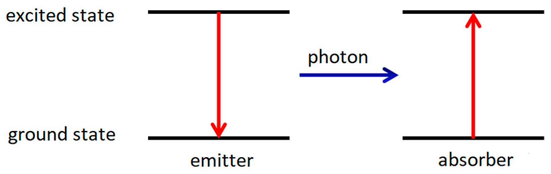
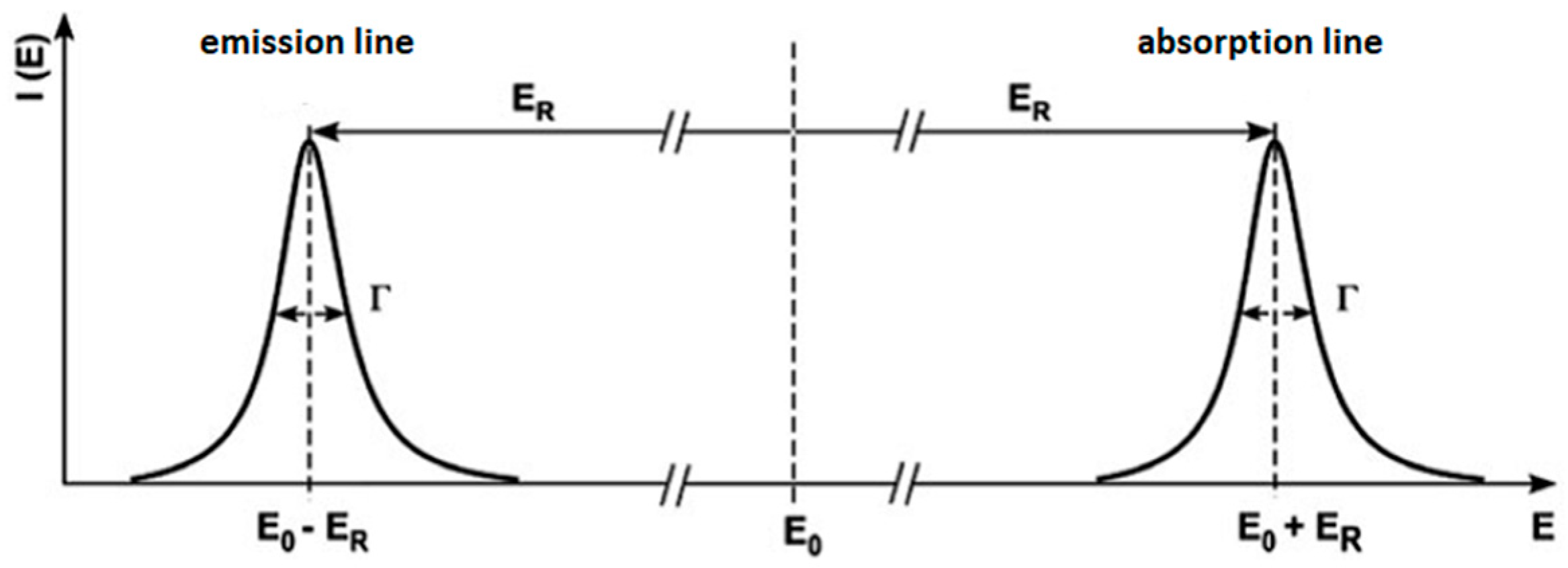
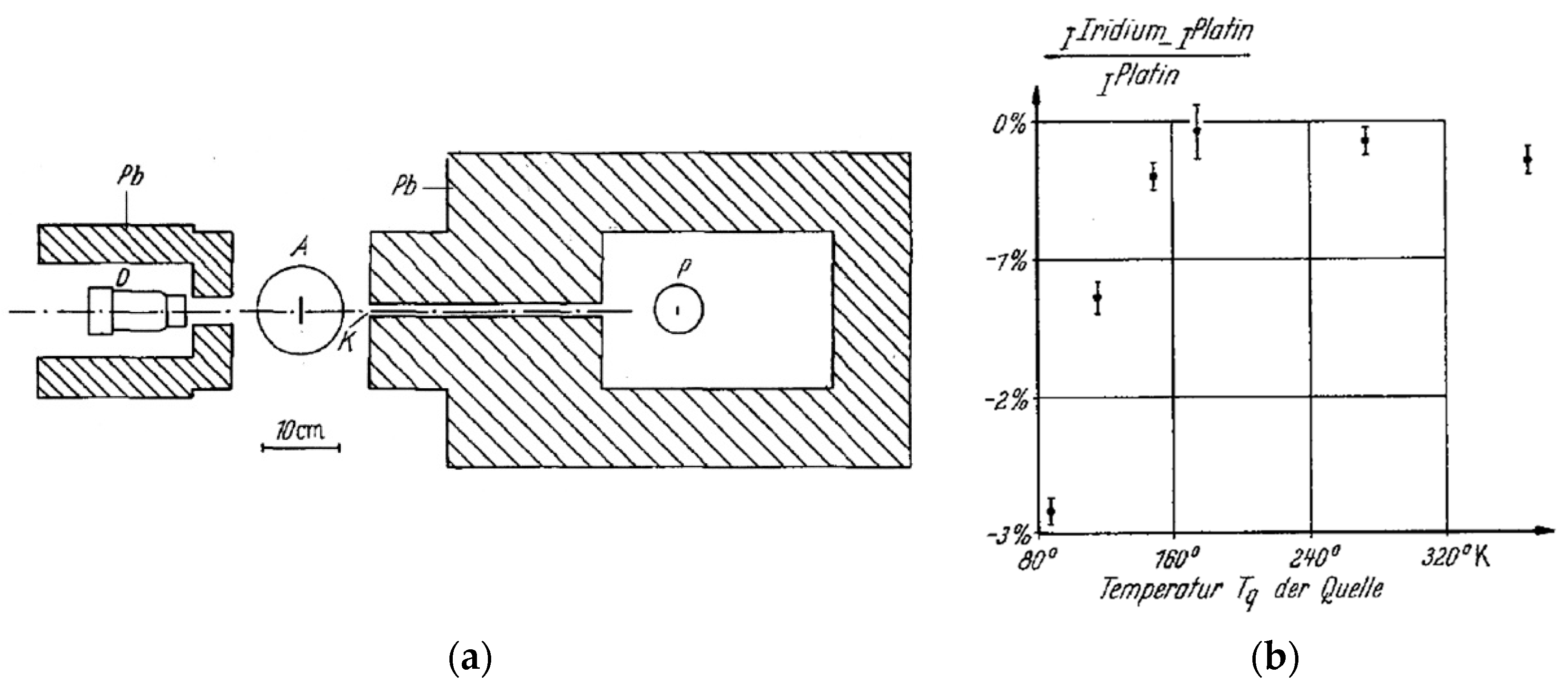
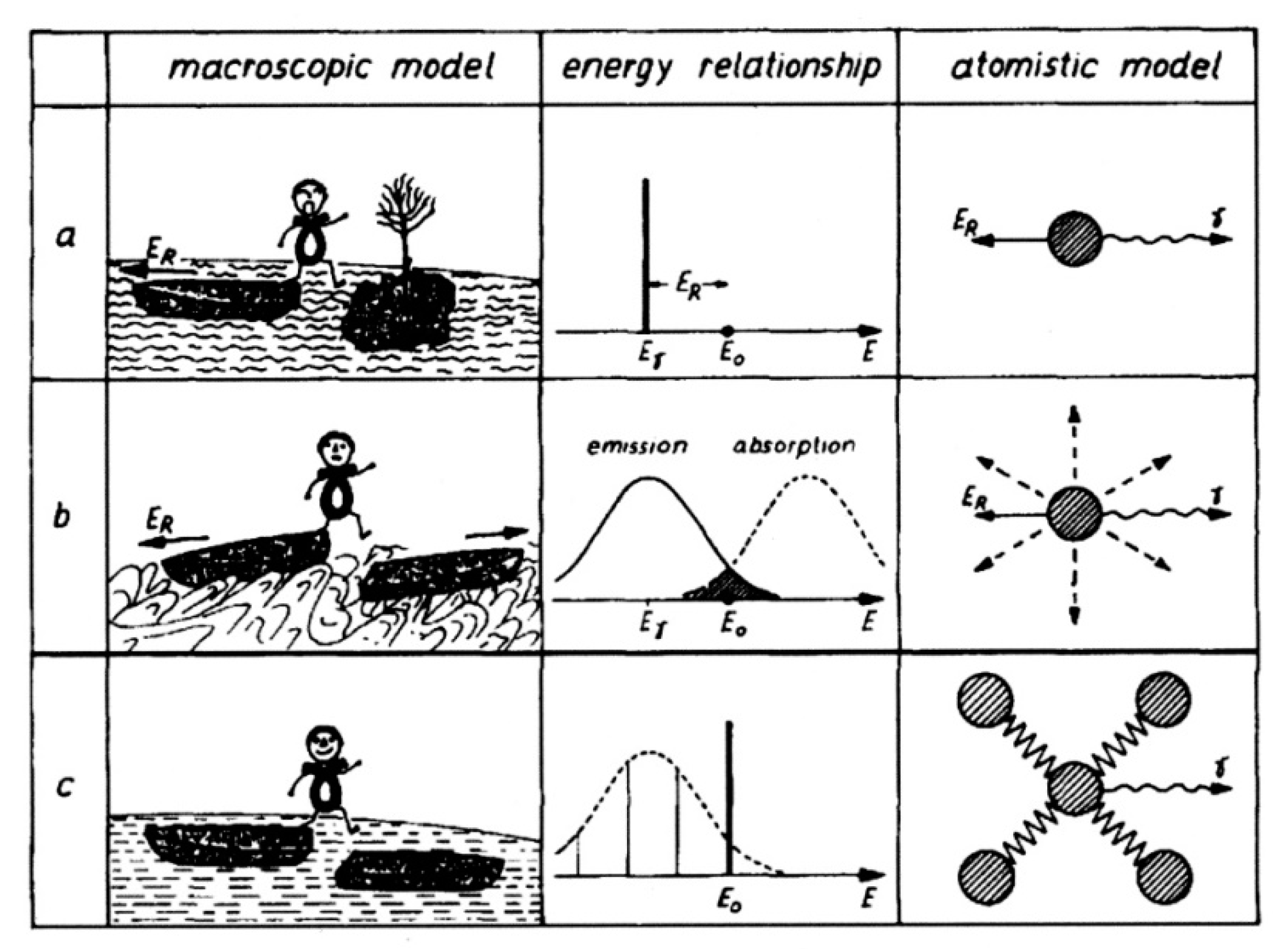
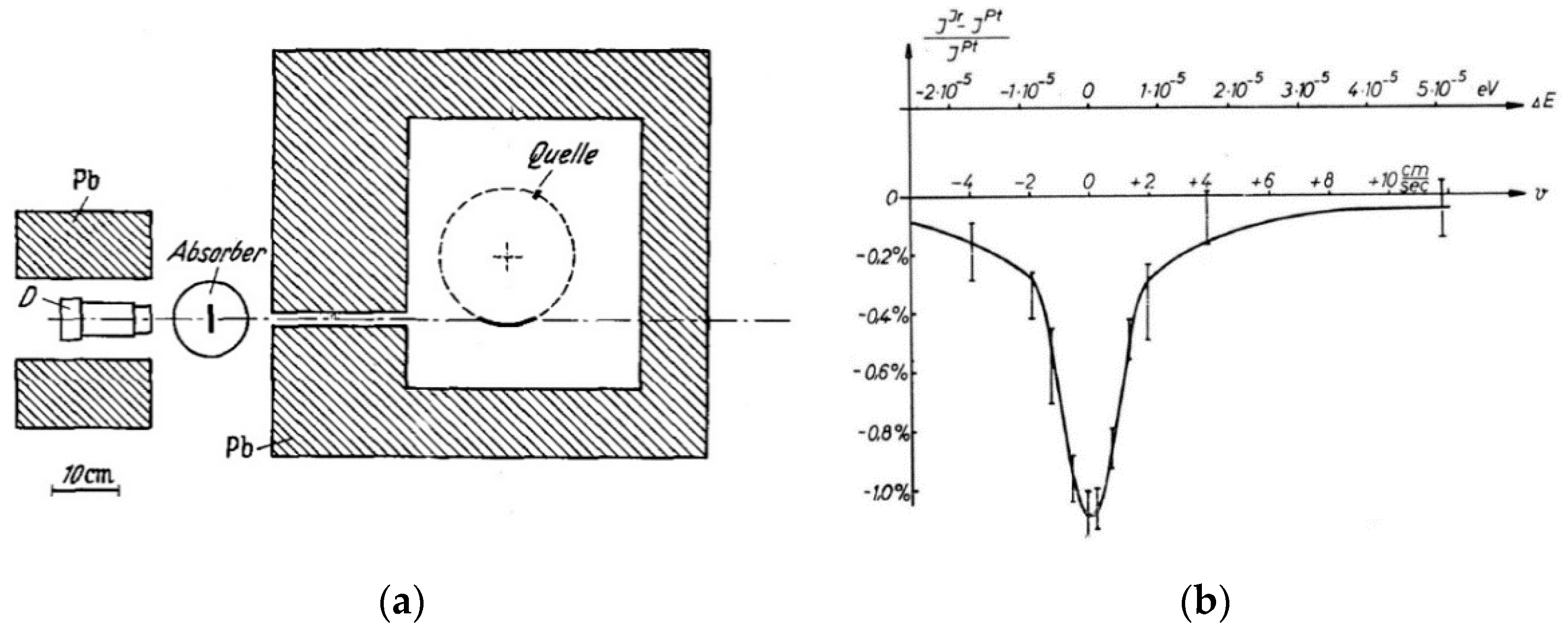
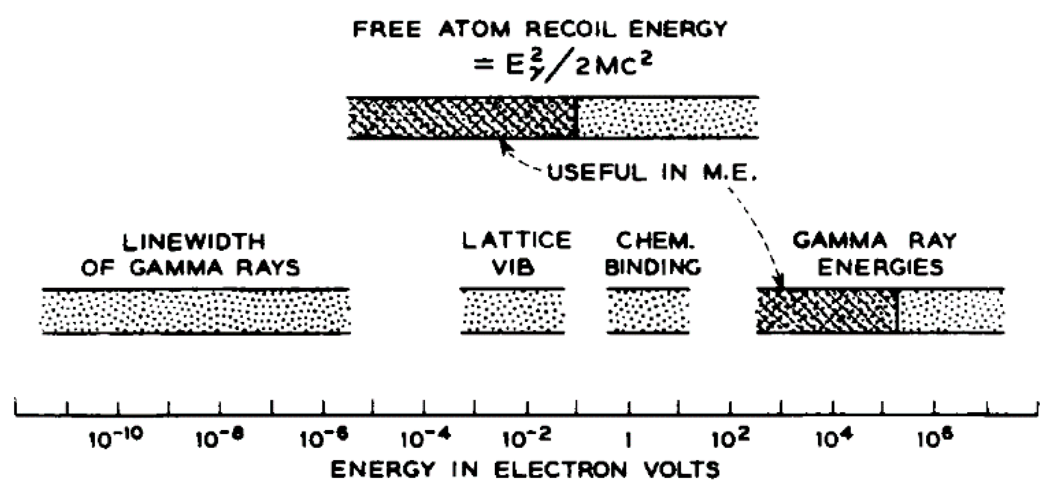
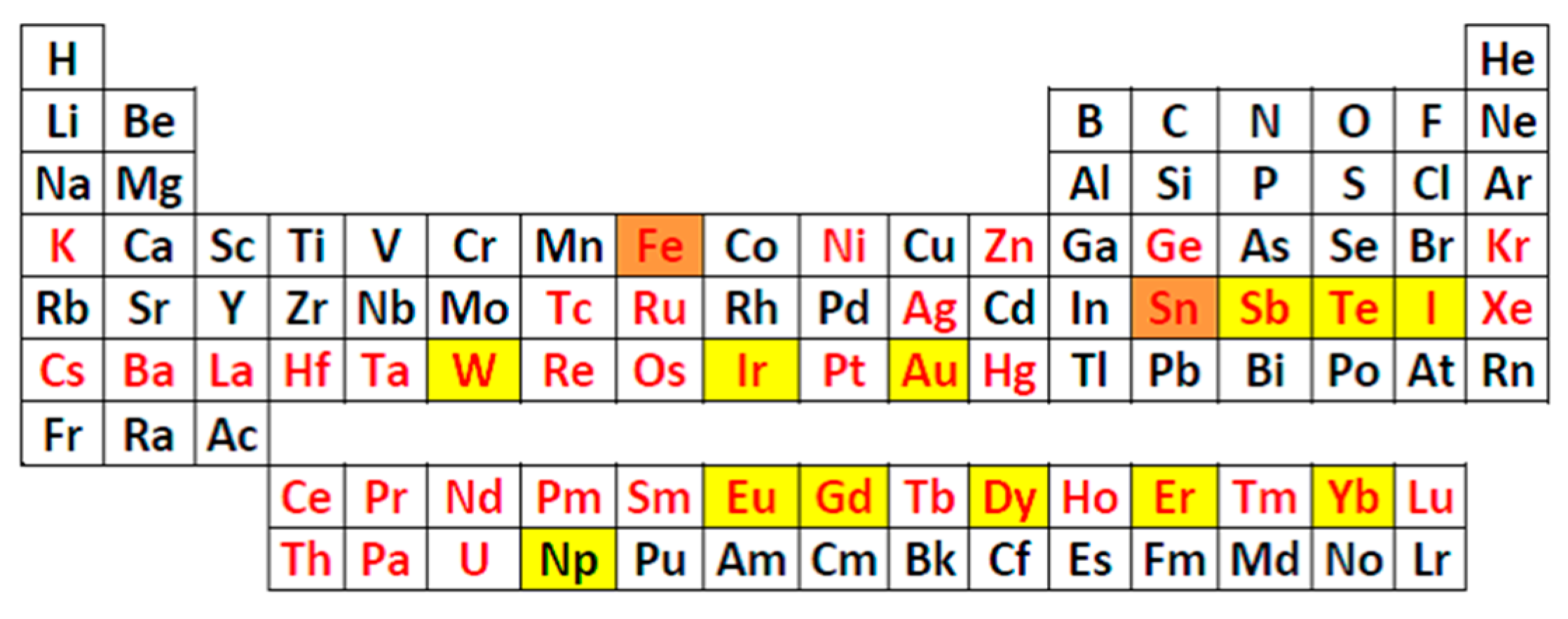
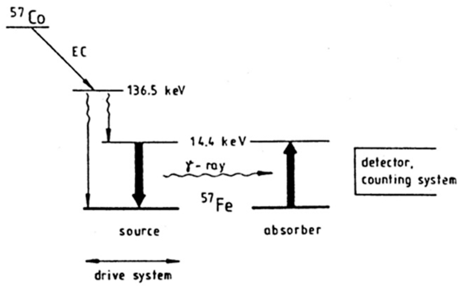
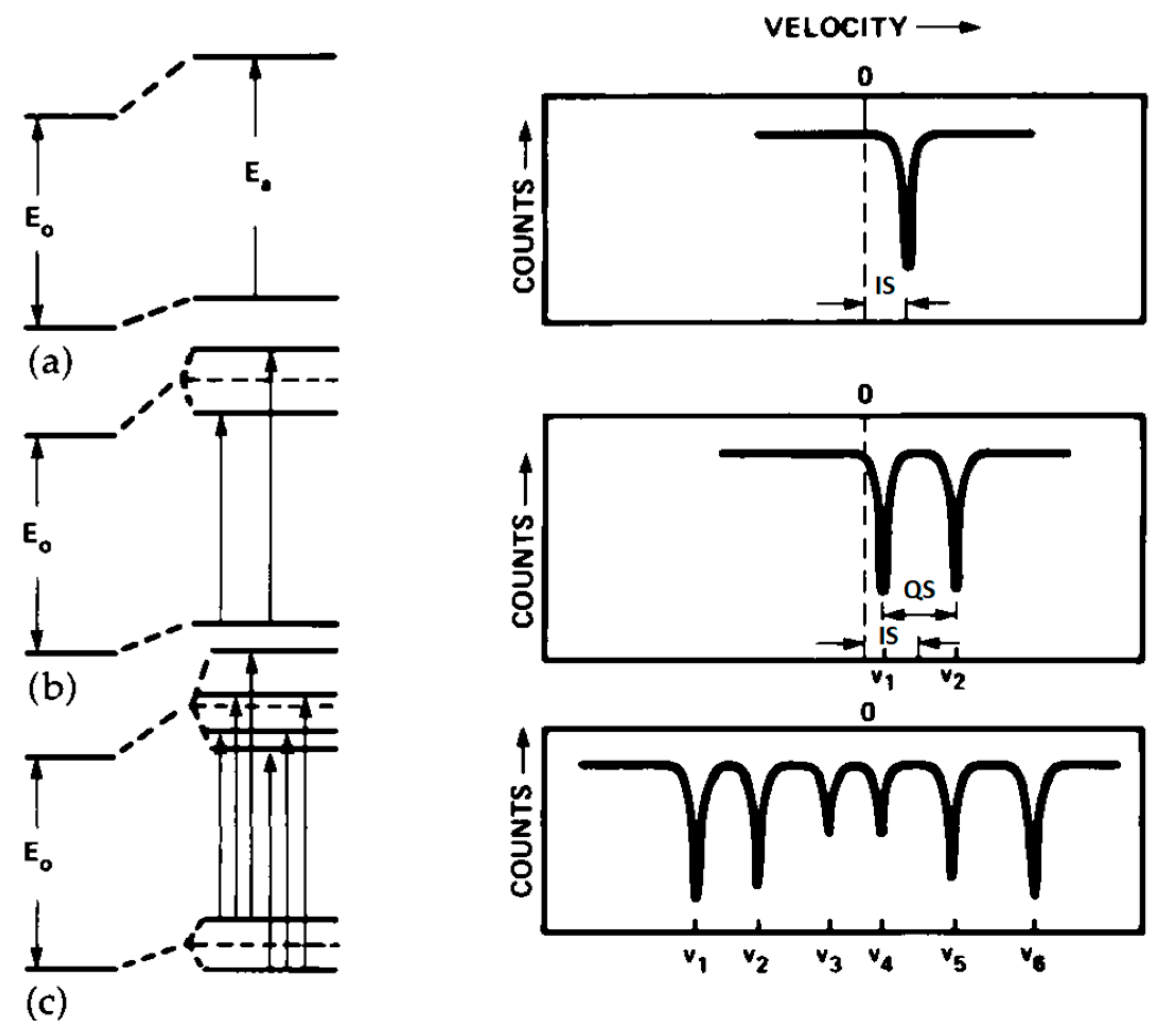
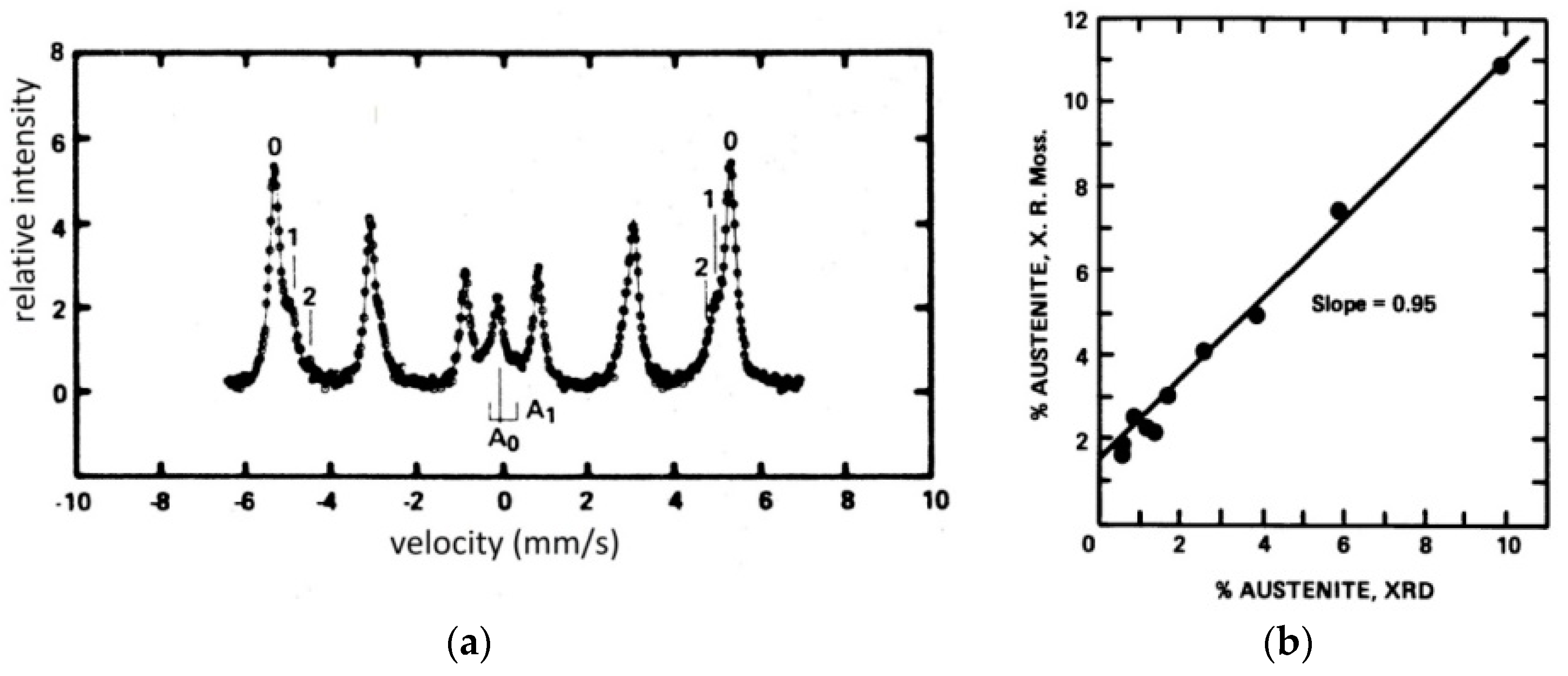
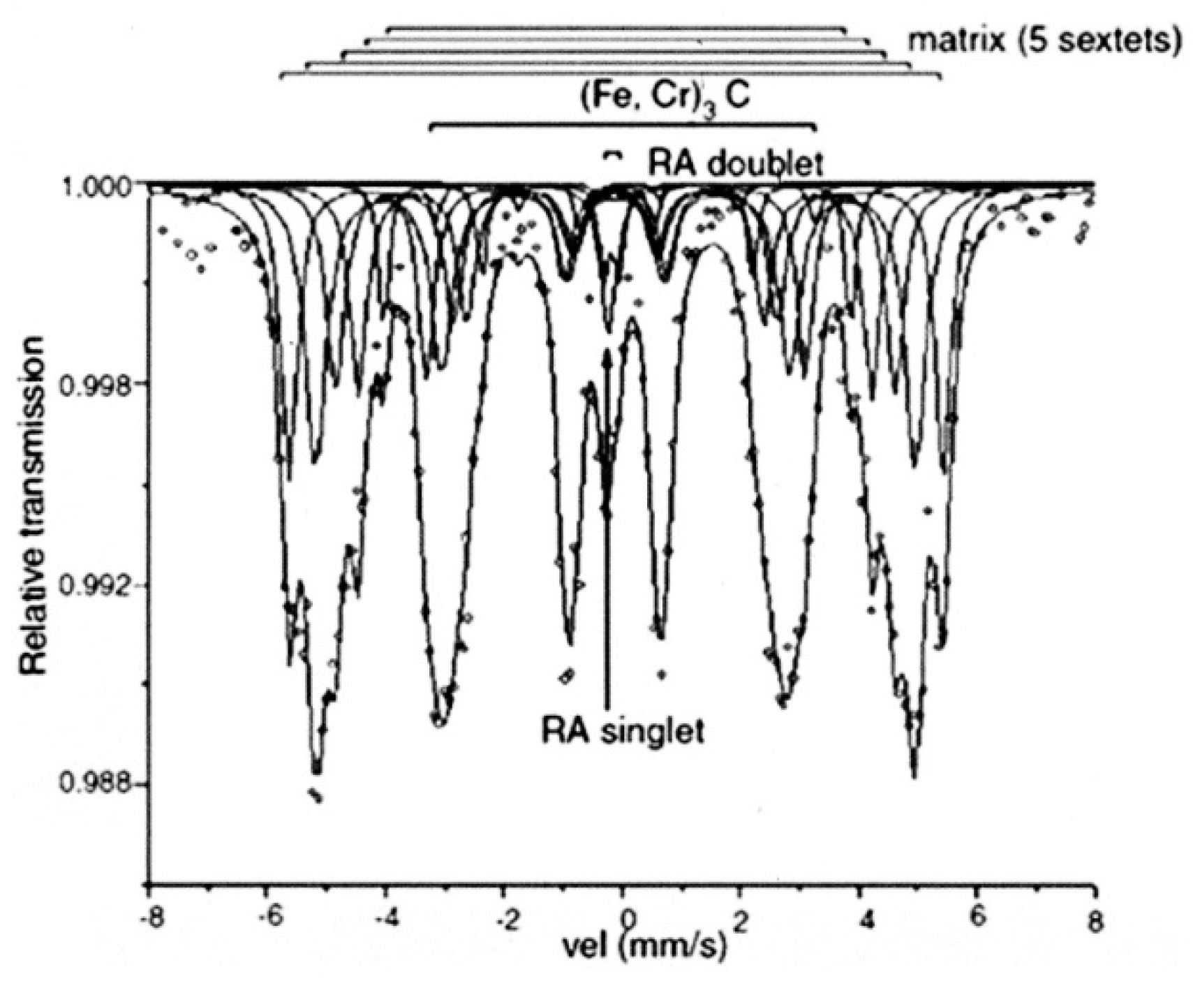
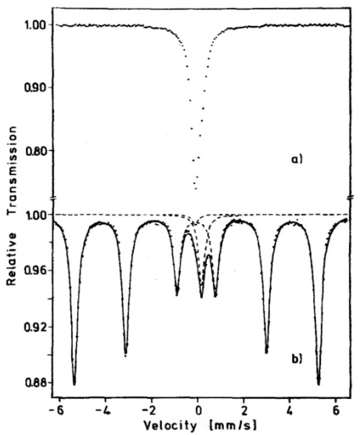
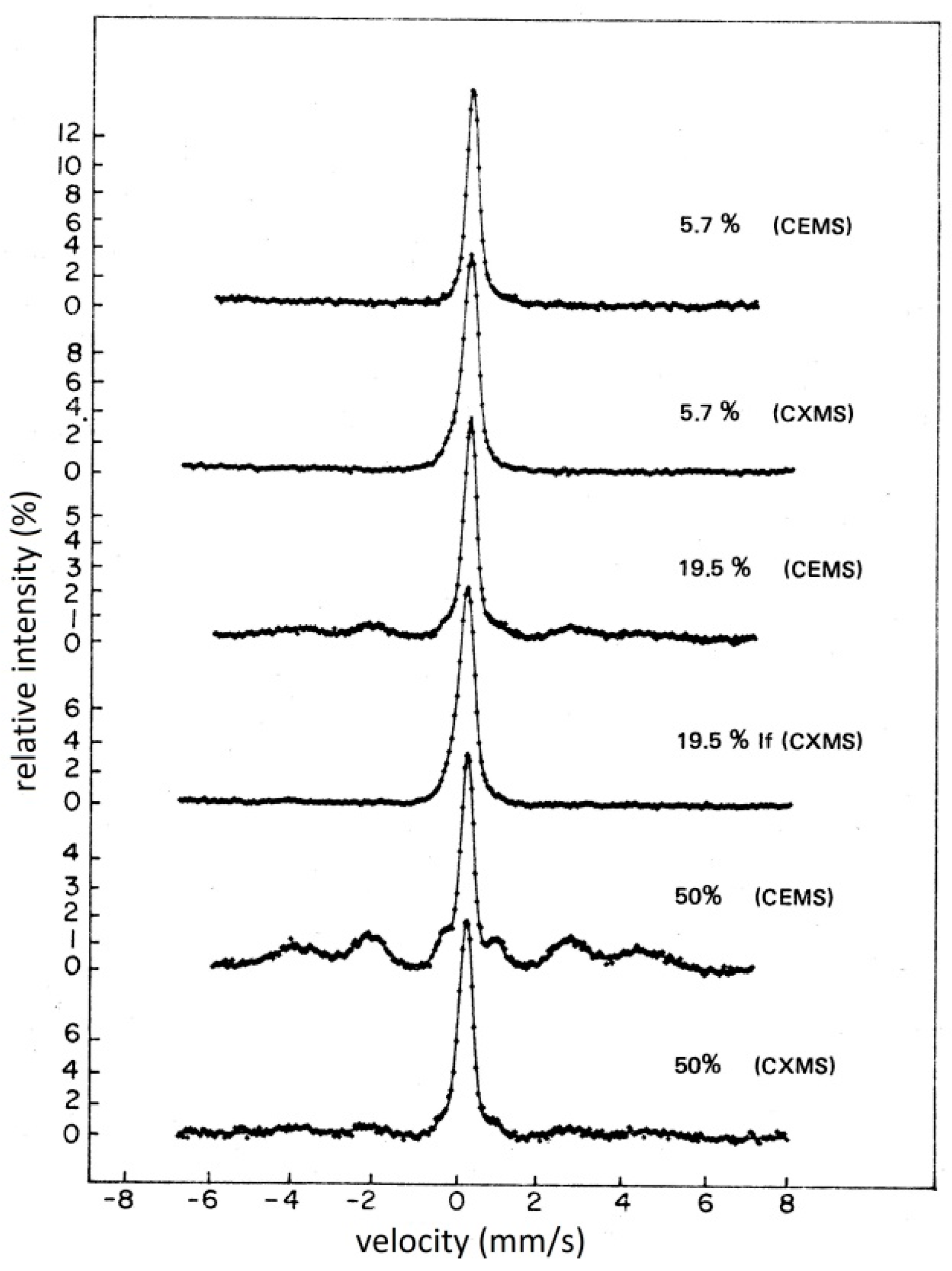
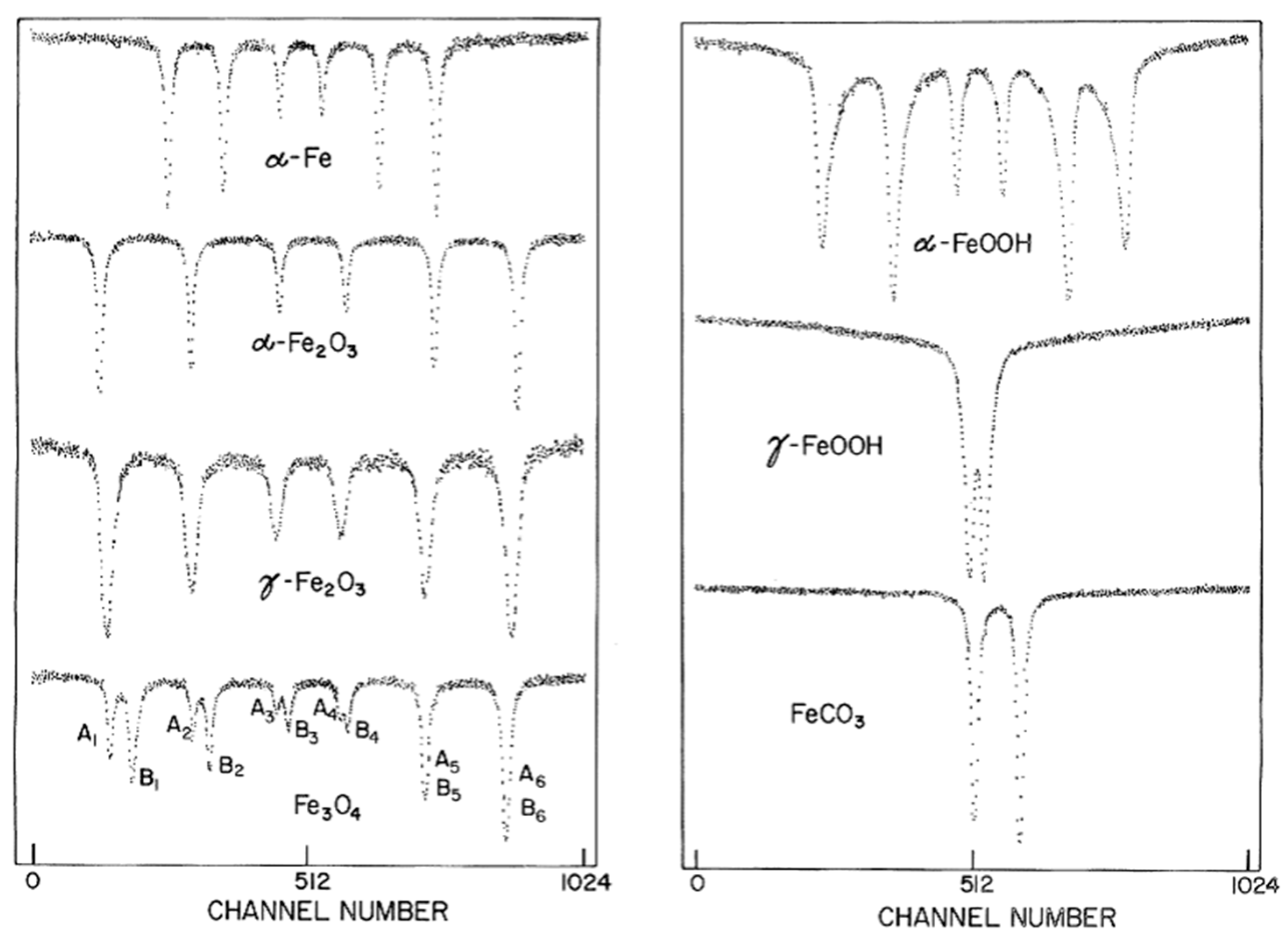
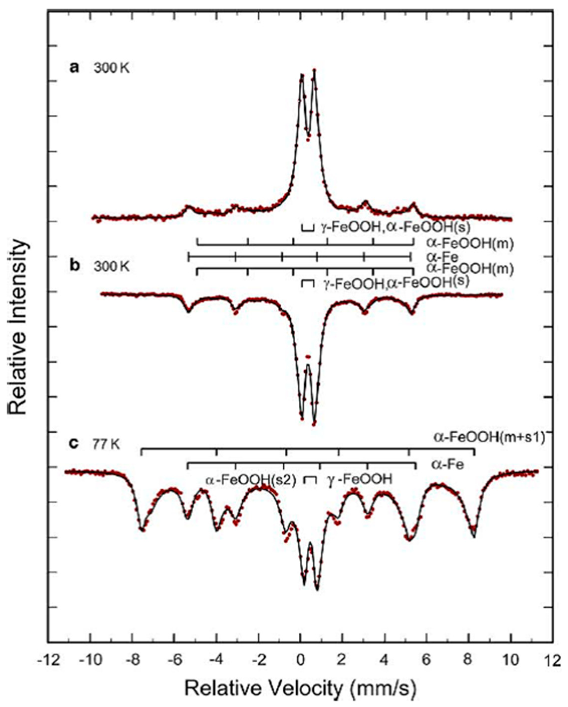
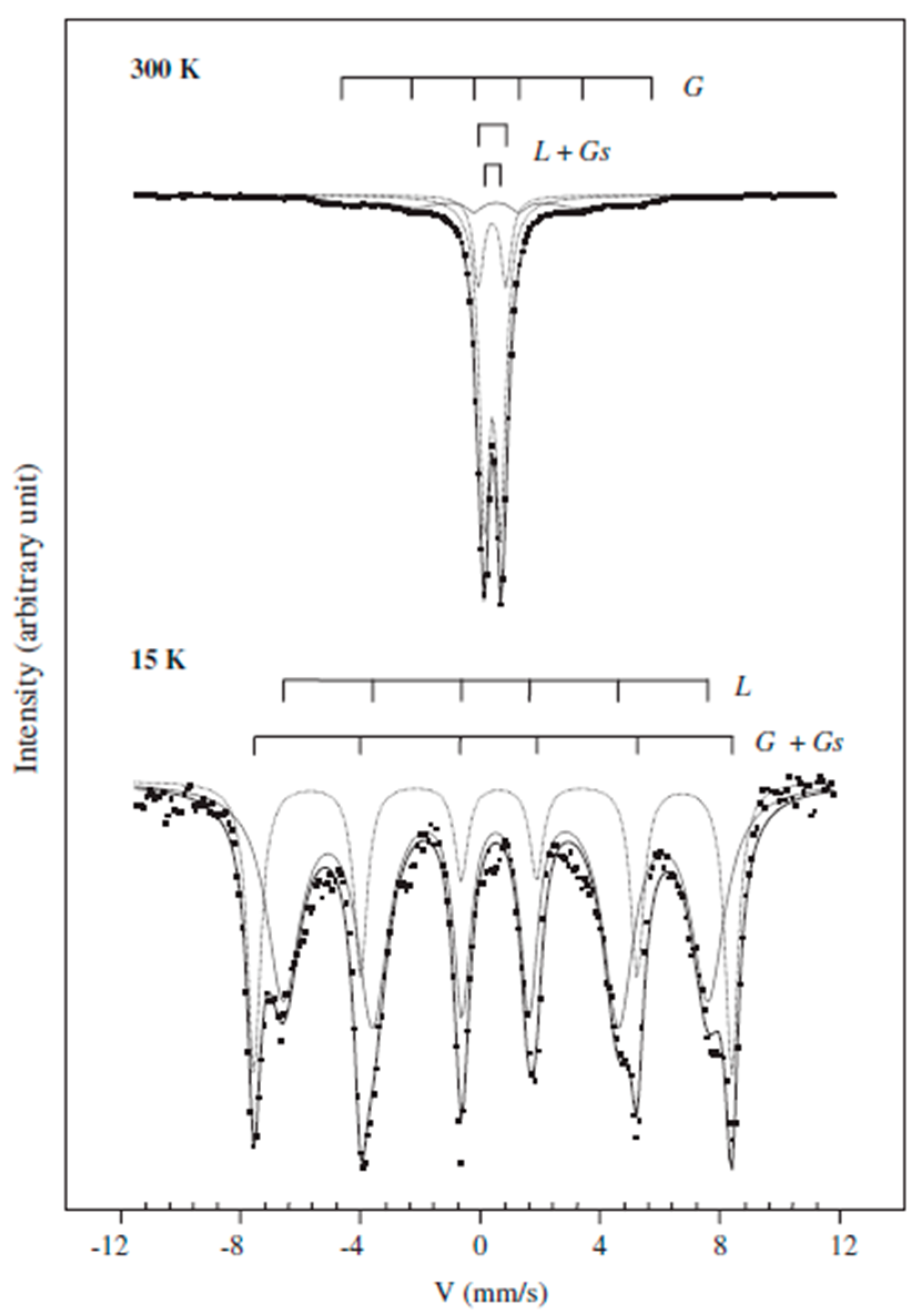
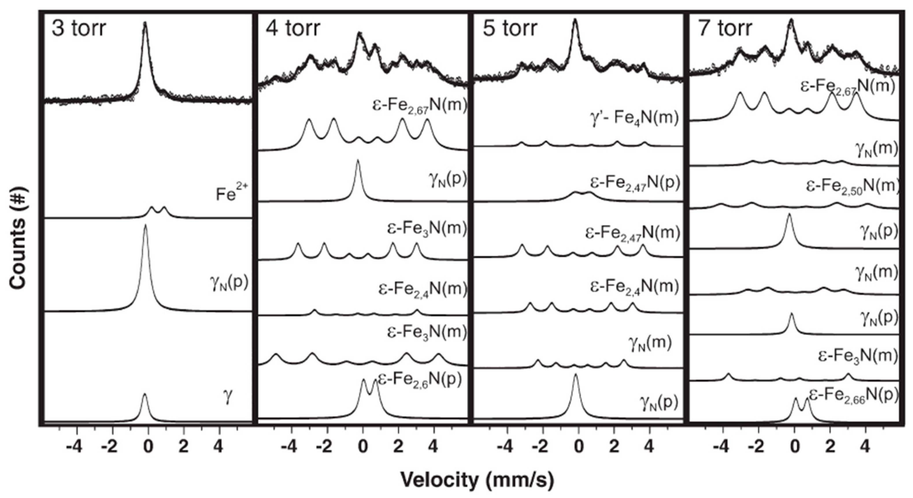
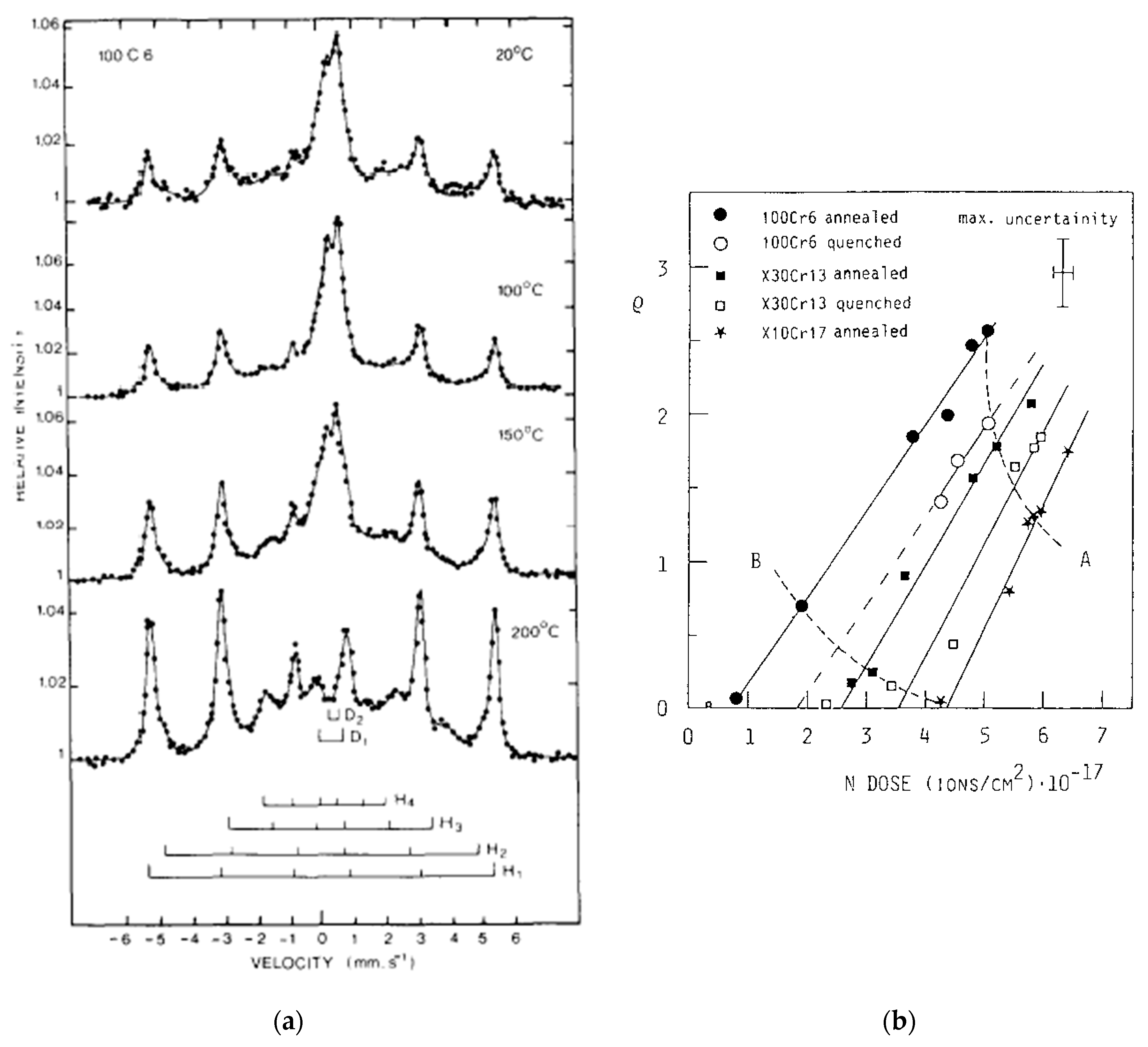
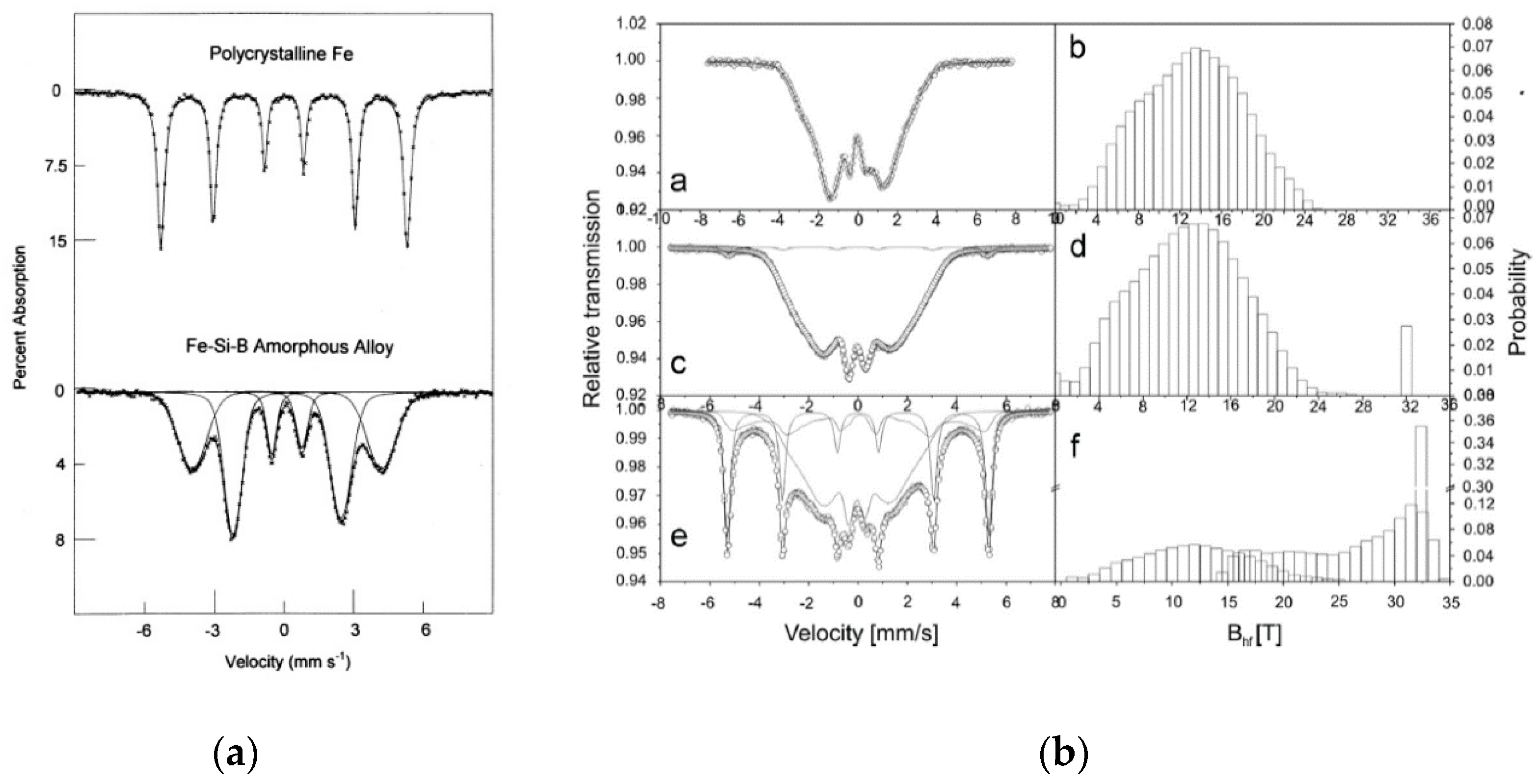
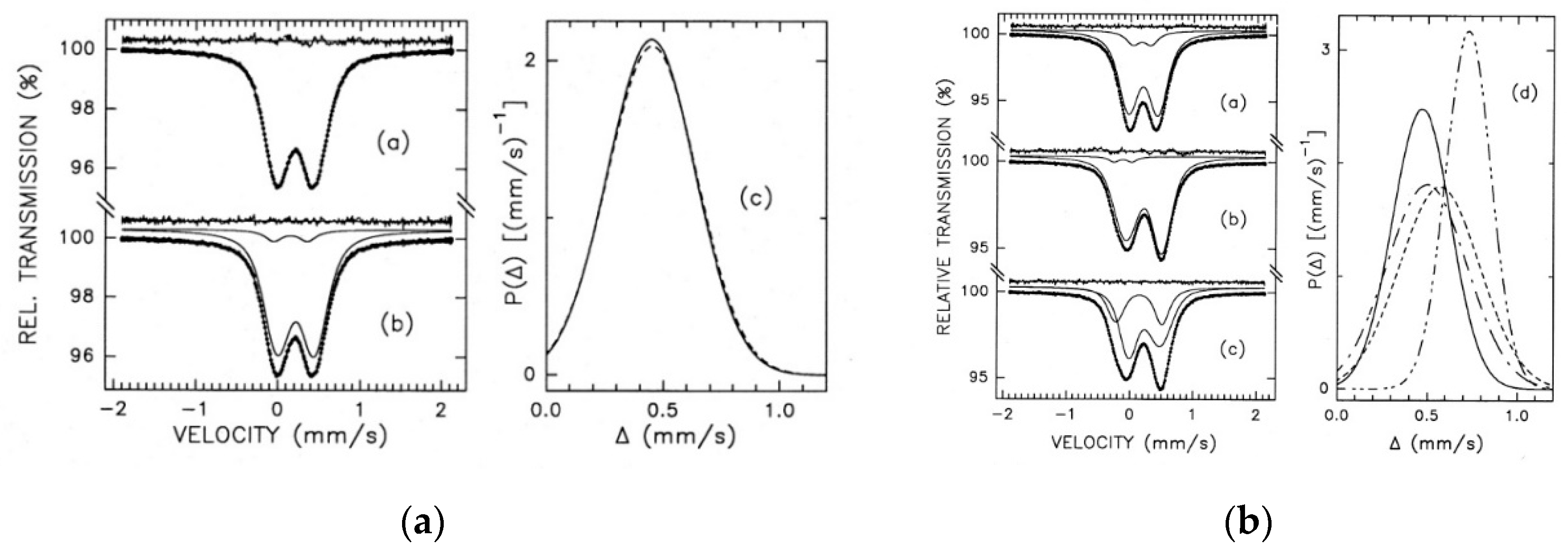
Table 1.
Orders of magnitude of energies (in eV) of optical and nuclear photons and of corresponding recoil energies and linewidths.
Table 1.
Orders of magnitude of energies (in eV) of optical and nuclear photons and of corresponding recoil energies and linewidths.
| Type of Radiation | Eγ | ER | Γ |
|---|---|---|---|
| optical photon | 1 | ~ | ~ |
| nuclear photon | ~ | ~ |
Table 2.
“Historical phases” of the Mössbauer effect. Reproduced from [25].
Table 2.
“Historical phases” of the Mössbauer effect. Reproduced from [25].
| Period | Date | Remarks |
|---|---|---|
| Prehistoric | Before 1958 | Might have been discovered, but wasn’t |
| Early Iridium Age | 1958 | Discovered, but not noticed |
| Middle Iridium Age | 1958–1959 | Noticed, but not believed |
| Late Iridium Age | 1959 | Believed, but not interesting |
| Iron Age | 1959–1960 | Wow!! |
Table 3.
Scheme of applicability of Mössbauer spectroscopy (MS) to materials science.
| Parameter | Origin | Information Obtainable |
|---|---|---|
| Isomer Shift | Interaction of nuclear charge distribution with the electron density at the nuclei in source and absorber (electric monopole interaction). | Valence. Kind of bonding. Nature of the electronic environment. Effect of internal pressure. Atomic volume. |
| Quadrupole Splitting | Interaction of the nuclear quadrupole moment with the electric field gradient at the nucleus (electric quadrupole interaction). | Quadrupole moment of the nucleus. Symmetry of the electronic environment. Nature and characterization of sites. Electronic properties. Effects of ordering and of impurities. Atomic clustering. Defects. |
| Internal Field | Interaction of the nuclear magnetic dipole moment with a magnetic field at the nucleus (magnetic dipole interaction, also called the nuclear Zeeman effect). | Nuclear spin. Magnetic ordering. Local magnetic moments. Phase analysis and changes. Superparamagnetism, effects of particle size. |
| Line Width and Shape | Local variations of resonance conditions. | Different types of local environment. Deviations from stoichiometry. Sample heterogeneities. Quantitative analysis. Local disorder. Relaxation effects. |
| Relative Intensity | Temperature. Effects of anisotropy and of polarization. | Quantitative analysis. Anisotropy and texture effects. Characterization of non-equivalent sites. Rate of transformations. |
Table 4.
Percent of martensite in steel strips measured after heat treatment with subsequent various degrees of cold working (cw) as measured by conversion electron Mössbauer spectroscopy (CEMS) and conversion X-ray Mössbauer spectroscopy (CXMS). Reproduced from [36], with perimisision from NDT International, 1977.
| Sample | Treatment | Martensite (%) | |
|---|---|---|---|
| CEMS | CXMS | ||
| AISI 321 | 1 h at 1050 °C | <1% | <1% |
| - | +5.5% cw | <1% | <1% |
| - | +19.5% cw | 33% | 7% |
| - | +50% cw | 61% | 32% |
© 2020 by the author. Licensee MDPI, Basel, Switzerland. This article is an open access article distributed under the terms and conditions of the Creative Commons Attribution (CC BY) license (http://creativecommons.org/licenses/by/4.0/).
Share and Cite
MDPI and ACS Style
Principi, G. The Mössbauer Effect: A Romantic Scientific Page. Metals 2020, 10, 992. https://doi.org/10.3390/met10080992
AMA Style
Principi G. The Mössbauer Effect: A Romantic Scientific Page. Metals. 2020; 10(8):992. https://doi.org/10.3390/met10080992
Chicago/Turabian StylePrincipi, Giovanni. 2020. "The Mössbauer Effect: A Romantic Scientific Page" Metals 10, no. 8: 992. https://doi.org/10.3390/met10080992
Note that from the first issue of 2016, this journal uses article numbers instead of page numbers. See further details here.