Implementation of Offshore Wind Turbines to Reduce Air Pollution in Coastal Areas—Case Study Constanta Harbour in the Black Sea

Abstract

Considering the current concerns regarding the level of air pollution from the Black Sea area, the aim of the present work is to establish whether a cold ironing project that involves the use of the wind resources from the port of Constanta (Romania) could become a reality. The regional and local wind resources measured at a height of 100 m above sea level were assessed by taking into account 20 years (2000–2019) of ERA5 wind data. The wind speed significantly increases as we move towards the offshore areas, with the wind Class C7 reporting a maximum of 41%. By combining the annual electricity production with the emissions associated with the port activities, it was possible to show that at least 385 turbines (each rated at eight MW) will be required to cover the electricity demand for this port. The present study has found it difficult to implement such a project based only on the available wind resources and has identified that more likely a mixed project that involves some other resources will be more appropriate. Finally, it is worth mentioning that the future of the ship industry is becoming greener and definitely, a wind project located near Constanta harbour will represent a viable solution in this direction.

1. Introduction

By analysing the global trade market one can easily notice that the maritime sector plays an important role in economic development. It is estimated that almost 80% of the global trades are transported by means of sea transportation. The sector is indeed very dynamic and has reported an annual increase of 3.2% between 2017 and 2020 [1]. On the other hand, industry is a major pollution source, and as a result, various legislative provisions have been introduced in order to protect the ocean environment and maritime resources. On a large scale, the CO₂ emissions associated with global warming are generated by navigation between ports, while on a local level, the port activities (also known as hoteling) are the main factors that have a negative impact on the human health around the port cities. If no significant change occurs, the air quality near the coastal cities will be significantly reduced due to the large nitrogen oxides (NOx) emissions, Particulate Matter (PM) and Volatile Organic Compounds (VOCs), respectively [2,3]. This problem is well known and most of the major harbour areas are under constant surveillance. This is the case for the Shanghai Port [4], Naples [5], Los Angeles [6] or Sydney [7], respectively.

Cold ironing or Onshore Power Supply (OPS) is one of the methods which could be used to help reduce local air pollution and improve the air quality near the coastal areas. OPS is used to describe the process of connecting a ship to a shore-side electrical supply in order to maintain the main function of a ship (ex: heating, refrigeration, emergency systems, etc.) at berth, during which time the engines are turned off. While the concept looks promising, with almost 6% of fuel consumption of a ship being allocated to the hoteling period, at the moment, only 30 ports are using this technology. The main challenges to be tackled for the use of such technology are related to the additional port installations and are caused by the fact that most of the operating ships are not equipped with systems compatible with the use of electricity from the shore [8]. Renewable energy sources (RES) represent an important part of the cold ironing process and their use has already been implemented at the port of Gothenburg (Sweden), which uses a shore-power source based on a local wind farm. By using this source, it is estimated that for the six weekly ships (Roll-on/Roll-off) connected to this project, an emission reduction of 80 metric tonnes for NOx, 60 metric tonnes—SOx and 2 metric tonnes for PM is expected [9]. The port of Hamburg (Germany) is considered another important project, where a significant part of the electricity demand is covered from wind and solar sources. For an initial investment of €4.8 million, it has been estimated that for the year 2014 almost two-thirds of the power consumption has been covered from natural sources or from additional combined heat and power plant (CHP) [10,11]. In Kotrikla et al. [12], the possibility of reducing the overall emissions for the port of Mytilene (Greece) was discussed. The study estimated that the total energy requirements of the operating ships could be covered by a hybrid project that included four wind turbines (rated at 1.5 MW) and a 5 MW photovoltaic system. In general, it seems that only a hybrid renewable energy system can support the activities of a port, this aspect being highlighted in Wang et al. [13]. The onshore and offshore wind resources from the vicinity of the Cartagena Port (Spain) [8] were also taken into account, with the main conclusions of the study being that energy consumption can be covered from a renewable project even during the winter time when the demand is much higher.

The Black Sea is one of the most polluted seas in the world and this is largely due to the emissions produced by ships, which are a significant contributor to the present situation. On a larger scale, three major air pollutant routes seem to emerge: (a) the south-western part of the Black Sea and Bosporus toward the Aegean Sea; (b) the south-eastern part of the Black Sea towards the eastern part of Turkey; and (c) the west to east area over the north of the Caucasus Peninsula. 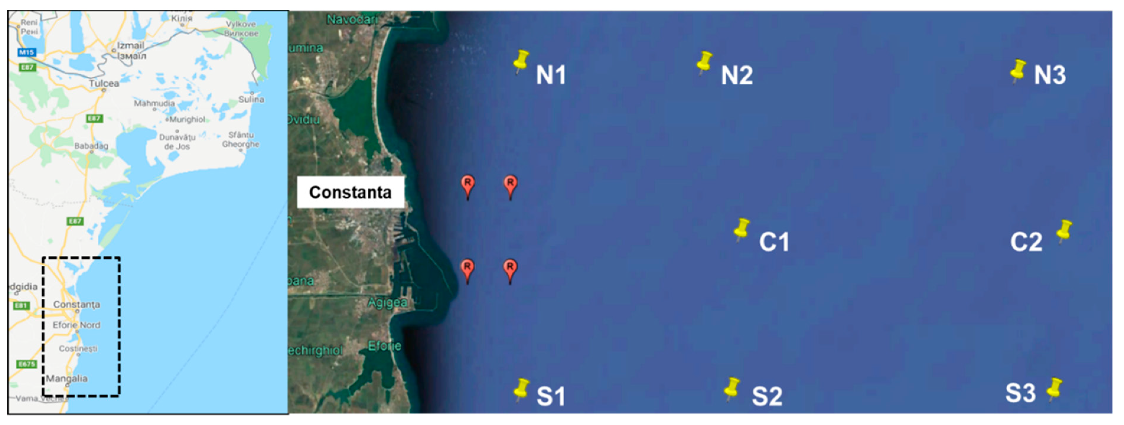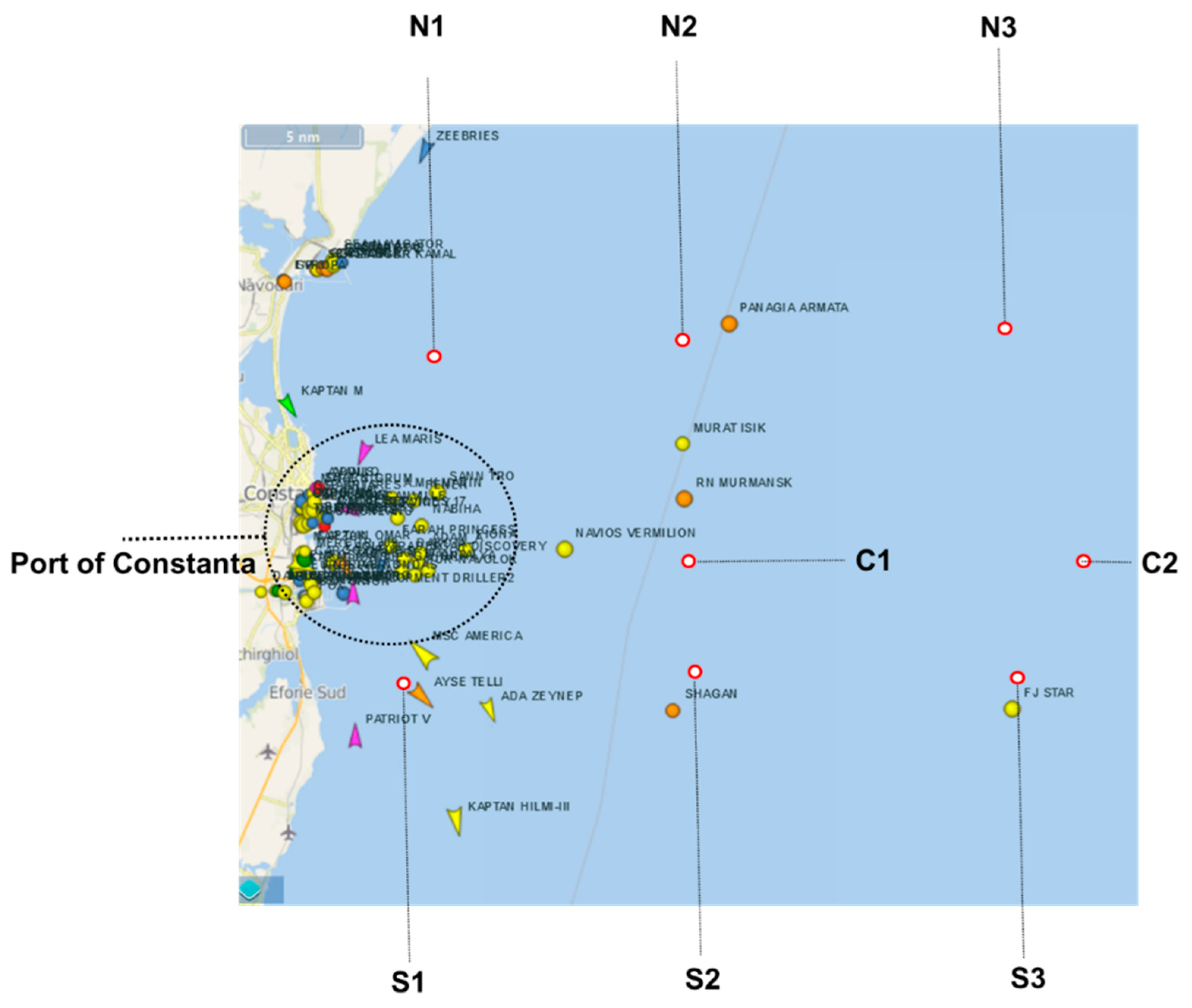In general, the movement of the air masses over the Black Sea area is quite complicated; however, it is estimated that the eastern coast of the basin will be more affected by these emissions, taking into account the strong winds that are coming from the northern part of the sea [14]. Coincidence or not, the north-western part of the Black Sea is transited by over 300 ships that connect the Romanian ports with the ports of Ukraine, Bulgaria and the Bosporus strait. The traffic related to this region represents almost 40% of the total traffic in the Black Sea. In addition, a significant percentage of the ships used for maritime traffic in this region (36% of ships) were built before 1990 when no emission regulations were imposed. Among Romanian ports, Constanta can be definitely mentioned as being the most significant and is on the 5th position on a European level in terms of the volume of cargo processed by the port services. In the near future, a further increase in activity can be expected for this port [15].

The Black Sea is also known for the wind conditions that can be used to power a wind farm, especially in the western part of this basin where the resources are more significant [16,17]. Onea and Rusu [16] provide a comprehensive assessment of the Romanian wind energy potential related to this coastal environment. The results of the assessment are reported at 80 m height (above sea level) and, according to their findings, the wind speed significantly increases as we go from onshore to offshore (ex: Saint George from 6 to 7.2 m/s). The best sites to develop a wind farm are located in the north (Danube Delta) and south (Vama Veche), but these areas are quite isolated and the grid-connection will be challenging. If we look at the Constanta site, we notice that a wind project may become profitable if located 20 km from shore (at least).

Some aspects related to the novelty of the present work are highlighted next. This work represents one of the first studies considering the use of the ERA5 wind data for a renewable analysis. Estimation of the wind turbines number required to support the Port of Constant’s activity represents another element of novelty, as well as the expected Levelized Cost of Energy (LCOE) values linked to a wind project that may operate in this coastal environment. Besides these particular aspects, the present work can also represent a general framework for the evaluation of how the offshore wind turbines can reduce air pollution in coastal areas, in general, and in the vicinity of the ports, in particular.

In this context, the following research questions will be addressed as part of the present work:

(a)

What is the best site to develop a wind farm near the Constanta Port?

(b)

How many wind turbines will be required to support a cold ironing project?

(c)

What is the expected cost of electricity generated from an offshore wind project?

2. Materials and Methods

2.1. Constanta Harbour

Constanta harbour can be found on the southern part of the Romanian coastline, being located between the port of Midia (north) and the port of Mangalia (south), respectively, as presented in Figure 1. The red points in the figure indicate the roadstead sector. By using this sector as a basis for the analysis, several reference points were defined at different distances from the shore, namely: 10 km—N1 and S1; 30 km—N2, C1 and S2; 60 km—N3, C2 and S3. A site located at 60 km from the shore can be still considered to be suitable for a wind project, taking into account that, at present, the average distance reported for the existing European wind projects is close to 59 km [18].

Table 1. Main characteristics of the Constanta sites considered.

No.	Long (o)	Lat (o)	Distance to Shore (km)	Water Depth (m) [19]
N1	28.786	44.284	10	30
N2	29.001	44.284	30	46
N3	29.368	44.276	60	50
C1	29.045	44.145	30	48
C2	29.422	44.143	60	56
S1	28.788	44.011	10	52
S2	29.033	44.012	30	38
S3	29.409	44.011	60	37

presents some additional information related to the points considered for evaluation, from which we can notice that the water depth is in the range 30–56 m.

In Figure 2 is presented a map of the ship traffic reported near the port of Constanta with the mention that the entrance in the berth area is made throughout the southern part of the port. Point S1 seems to block the entrance from the port, so in this case, a wind farm located onshore seems to be more indicated. The remaining points are located outside the roadstead sector, so various spatial wind farm configurations can be designed in order to avoid the main ship routes.

A first glimpse of the Romanian port activities is provided in Figure 3, from which it can be noticed that the port of Constanta is by far one of the busiest ports in the region. Although the port of Midia also reported higher numbers for the ships defined by capacities located below 5000 tonnes, in general, the value does not exceed 150 tonnes. The port of Mangalia reports lower activities that can go to a maximum of 89 events (ships < 5000 tonnes), while for example a maximum of 6 activities was reported for larger ships (90,000–18,000 tonnes). Going back to the port of Constanta, we can notice that this is a dynamic environment, which is frequently used by ships that have capacities in the range of 5000 and 20,000 tonnes. In addition, the events in the port of Constanta also involve larger ships (>90,000 tonnes), with a significant increase from 76 (in 2011) to 124 events being reported at the end of 2019. On the contrary, the number of events involving smaller ships (<5000 tonnes) is significantly decreasing from 2687 (year 2011) to 1515 stops reported at the end of 2019.

Figure 4 presents a short description of the Constanta harbour activity, including the ship traffic [21] and the associated air pollution resulting only from the port activities [22]. By looking at this data, we can notice that the traffic associated with this port is growing from one year to another, starting from 4763 kilotons (in 2010) and reaching a maximum of 66,603 kilotons (+40%) at the end of 2019. This trend is also reflected in the level of air emissions where at the end of 2010 the values were close to 5.52 kilotons, gradually increasing to 6.89 kilotons (year 2016: +25%) and 7.71 kilotons (year 2019: +40%). It is important to mention that a significant share is covered by NOx emissions (almost 80%). From the literature review, only the air emissions from the interval of 2010 to 2016 were mentioned, while the expected values for the years 2017, 2018 and 2019 were estimated in order to highlight the ascendant trend.

2.2. Wind Data

The ERA5 is one of the newest projects maintained by the European Centre for Medium-Range Weather Forecasts (ECMWF) being designed to replace the old ERA-Interim project. Some new improvements were made, as: the covered period was extended to 1950–present; the spatial resolution was increased; temporal resolution is set to hourly values; various newly reprocessed datasets and recent instruments were considered; a new assimilation system is used—IFS Cycle 41r2 4D-Var [23,24]. For this work, only the 20-year time interval from January 2000 to December 2019 were processed for the Constanta sector, since this is the expected design life of a wind farm [25,26]. The wind speed is processed at 10 m height (above the sea), being defined by a spatial resolution of 0.25° × 0.25° and a temporal resolution of 6 h (four values per day, 00-06-12-18 UTC—Coordinated Universal Time, respectively). Although a higher output resolution is available, according to the documentation of this ERA5 project the results will be the same and will not contain any extra information, just that the interpolation process will be carried out on a higher resolution [27].

The wind industry is changing and this effect is more visible on the offshore areas, being expected larger turbines and much higher hub heights. In previous studies, a hub height of 80 m (U80) was considered as standard [28,29] while at this moment most of the studies are focused on the 100 m height (U100) [30,31,32]. In order to make this adjustment, the following equation can be considered [33]:

$$U100=U10\frac{\ln \left(z_{100}\right)-\ln \left(z_{10}\right)}{\ln \left(z_{10}\right)-\ln \left(z_0\right)},$$

(1)

where U100 is the wind speed at 100 m height of (z₁₀₀); U10 represents the initial wind conditions at 10 m (z₁₀), while z0—is the roughness factor (calm sea surface—0.0002 m).

2.3. Wind Turbines

For the current evaluation, five different wind turbines (denoted from A to E) will be used to identify electricity production, their characteristics being indicated in

Table 2. Technical specifications of the selected wind turbines [16,35].

Turbine	ID	Rated Power (MW)	Cut-In Speed (m/s)	Rated Speed (m/s)	Cut-Out Speed (m/s)	Hub Height (m)
General Electric GE 2.5	A	2.5	3	13	25	100
Siemens SWT 3.6	B	3.6	3.5	14	25	100
Areva M5000	C	5.0	4	12.5	25	100
Siemens SWT 6.0	D	6.0	4	13	25	100
Vestas V164	E	8.0	4	13	25	100

and Figure 5. The rated capacity of the turbines covers the interval of 2.5–8 MW, being possible to assess in this way the performances of some operational wind farms that include low capacity turbines, and also of some future projects that are based on high capacity generators. Although each turbine is characterised by particular hub heights, for consistency the performances of all the systems will be evaluated at 100 m height.

The turbines are related to: turbine A—General Electric GE 2.5 (General Electric, Boston, MA, USA); turbine B—Siemens SWT 3.6 (Siemens, München, Germany); turbine C—Areva M5000 (Areva, Paris, France); turbine D—Siemens SWT 6.0 (Siemens, München, Germany); turbine E—Vestas V164 (Vestas, Aarhus N, Denmark).

The Annual Electricity Production (AEP) of a wind generator can be estimated as [34]:

$$\mathrm{AEP}=T\times {{\displaystyle \int }}_{cut-in}^{cut-out}f\left(u\right)P\left(u\right)du,$$

(2)

where AEP is defined in MWh; T—average number of hours per year (8760 h/y); f(u)—Weibull probability density function; P(u)—power curve of a turbine; cut-in and cut-out—the turbine characteristics.

The Weibull PDF (probability density function), is defined as [36]:

$$f\left(u\right)=\left(\frac{k}{c}\right){\left(\frac{u}{c}\right)}^{k-1}exp\left[-{\left(\frac{u}{c}\right)}^k\right],$$

(3)

where u—wind speed; k—the shape parameter; c—the scale parameter (in m/s).

Another objective of the present work is to identify the economic viability of an offshore wind project by using the Levelized Cost of Energy (LCOE). This includes the CAPEX (Capital Expenditure) and all OPEX (Operational expenditures) values, divided by the electricity produced by a project during a particular time interval. This can be expressed as [37]:

$$\mathrm{LCOE}=\frac{\mathrm{CAPEX}+{{\displaystyle \sum }}_{t=1}^{\eta }\frac{{\mathrm{OPEX}}_t}{{\left(1+r\right)}^t}}{{{\displaystyle \sum }}_{t=1}^{\eta }\frac{{\mathrm{AEP}}_t}{{\left(1+r\right)}^t}},$$

(4)

where: OPEX_t—Operational expenditures reported for year t; AEP_t—Annual Energy Production corresponding to year t; r—the discount rate; η—lifetime of the project; t—year from the start of the project. Taking into account that the cost of an offshore project is influenced by the water depth and distance from the shore, a cost-scaling factor [38] was applied to each point, namely: 1.08—N1; 1.252—S1; 1.29—rest of the points.

In order to establish the equivalence between the CO₂ emissions associated with the Constanta air pollution and the AEP production, the following equation was considered [39]:

$${\mathrm{CO}}_{2\mathrm{emissions}}=\mathrm{AEP}\times x\times y,$$

(5)

where: CO_2emissions—emission rate (in tonnes CO₂/MWh); AEP—Annual Energy Production (in MWh); x —reductions of kilowatt-hours into avoided units of carbon dioxide emissions (x = 6.62 × 10⁻⁴); y—convert metric tonnes to tonnes (y = 1.102311).

3. Results

3.1. Assessment of the Wind Conditions

Figure 6 presents the spatial distribution of the U100 parameter over the entire Black Sea area, being also included in the reference points from the Constanta sector. According to these values, the areas located in the central part of this basin reveal the best conditions for the development of a wind project (U100 > 8 m/s) at which we can add the Azov Sea. By looking at the Romanian coastal area, we may notice that the wind conditions reveal much higher values than the Bulgarian area, but are below the values reported near the Crimea Peninsula that frequently report values of 7 m/s.

The seasonal differences (in %) reported by the western region were computed in Figure 7, where the Romanian sector was highlighted. During the spring time there is an attenuation of the wind conditions that can go up to 10 or 15% compared to the total time, while the central part of the Black Sea seems to reveal no variation. A similar trend is reported for the summer time, where the Romanian sector is associated with a decrease that goes up to 15%, compared to the southern part where a slight increase of the values can be noticed (+5%). As for the autumn time, the entire region is defined by positive values that can go up to 10% near the coastal areas, while for the southern region a 5% can be considered more representative. Much higher variations (positive) are expected during the winter season, when the Romanian sector reports values close to 15%, while as we go north a maximum of 20% may be noticed near the Ukrainian waters.

Figure 8 presents the Weibull distribution of the considered points, including the specific parameters (c and k). Although the points are located in a relatively small area that defines the Constanta sector, we can notice that there are significant variations especially in the case of the scale parameter. For the N-points close to the shore, a value of 6.97 m/s (N1) is noticed, which gradually increases to 7.99 and 8.35 m/s in the case of N2 and N3, respectively. Compared to these values the S-points reveal slightly higher values (+1.62%), that go up to: S1 = 7.05 m/s, S2 = 8.12 m/s and S3 = 8.46 m/s, respectively.

The wind energy potential of a particular site can be evaluated throughout wind classes [35], that can go from C1 to C7, a higher class being considered a good indicator.

Table 3. Percentage of wind classes for the U100 parameter, corresponding to the 20-year time interval of 2000–2019.

Site	Wind Class (%)
	C1	C2	C3	C4	C5	C6	C7
N1	38.7	11.4	7.79	5.8	5.21	7.17	23.9
N2	30.1	9.68	6.56	5.5	5.16	7.41	35.6
N3	28.2	8.17	6.12	4.93	4.97	7.22	40.3
C1	29.5	9.31	6.52	5.27	5.12	7.28	37
C2	28.3	8.23	6.11	5.02	4.86	7.1	40.4
S1	38.5	11	7.45	5.86	5.28	7.21	24.8
S2	29.7	9.25	6.59	5.01	5.23	7.33	36.9
S3	27.7	8.3	6.11	4.81	4.87	7.23	41

Wind class (U100): C1 ≤ 5.05 m/s; C2 = 5.05–5.86 m/s; C3 = 5.86–6.43 m/s; C4 = 6.43–6.89 m/s; C5 = 6.89–7.35 m/s; C6 = 7.35–8.04 m/s; C7 ≥ 8.04 m/s.

presents such an analysis, where the wind conditions were reported to U100 by using Equation (1).

Generally, the distribution is divided between two dominant classes, namely C1 and C7, being expected values of 38.5% close to the nearshore points (N1 and S1) and maximum of 41% offshore (S3). The nearshore points (N1 and S1) present much higher values in Class C1, but as we exceed 30 km from shore, Class C7 starts to become dominant gradually increasing to 35.6% (N2) and 40.3% (N3). By looking at the central points, we may notice that Point C1 that is located on the same distance to shore as N2 and S2, presents slightly better values for Class C7 (37%).

Considering that in the introduction part was briefly mentioned that the pollutants from the port of Constanta could be transported by the air masses in the other regions of the Black Sea, in Figure 9 is presented the monthly distribution of the wind roses reported by Site C1. The results are indicated in terms of the wind classes (U100) mentioned in Table 3. From the analysis of the wind classes, we can notice that the values are divided between the C1 and C7 classes, as expected during the wintertime being expected conditions that are more energetic. In terms of the direction, it seems that, in fact, there are periods when the wind is clearly blowing from offshore to onshore (ex: July, August, October, December). Another dominant pattern is for the wind that blows from the south-west sector, this being the case of May, April or November. According to these results, there is no clear evidence that the emissions from this area will affect the eastern coast of the Black Sea.

3.2. Wind Turbine Performances

Figure 10 reveals the distribution of the AEP for all the turbines where, as expected, the performance is directly related to the expected rated power of each system. The reported values oscillate between: N1 = 5082–14,396 MW; N2 = 6805–20,030 MW; N3 = 7511–22,386 MW; C1 = 7016–20,730 MW; C2 = 7521–22,423 MW; S1 = 5208–14,810 MW; S2 = 7028–20,768 MW; S3 = 7673–22,917 MW. According to these data, much better performances are being related to Site S3.

The annual variation of the AEP indicator is presented in Figure 11, only for Turbine C (Areva M5000-116), the rest of the turbines are supposed to reveal a similar trend, higher or lower values associated with their rated power. The differences between the sites are more visible in this case, with the mention that Site N3 shows a similar plot as the one reported for C2. Although the values are in general constant, there are noticed some peaks, such in the case of the year 2001 or for the year 2011 where a sharp decrease may occur.

The capacity factor (Cf) is a frequently used parameter that can identify the reliability of a wind turbine, being defined as [16]:

$$C_f=\frac{P_{turbine}}{Rate{d}_{power}}\times 100,$$

(6)

where: P_turbine—indicates the electric power produced by each system, and Rated_power—the rated power of each turbine.

Figure 12 presents the monthly distribution of this parameter, considering only Turbine C. The results can be divided into two distinct periods, namely: October–March (higher values) and April–September (lower values). A maximum of 49% may be reported during the winter months, but on average the values do not exceed 30%. Better performances are being expected near the sites S3, C2 and N3, while on the opposite side, Points S1 and N1 reveal the lowest values (ex: 32% in February or 13.7% in June).

Table 4. Turbines performances (U100) evaluated for the 20-year time interval of 2000–2019. Only the minimum and maximum values are indicated for each turbine (A, B, C, D or E).

Site	AEP (MWh)	Capacity Factor (%)	Operating Capacity (%)	Rated Capacity (%)
N1	5082 (A)–14,396 (E)	19 (B)–23.2 (A)	75.7 (CDE)–87.3 (A)	2.33 (ADE)–3.04 (C)
N2	6805 (A)–20,030(E)	26.2 (B)–31.1 (A)	81.3 (CDE)–89.9 (A)	5.57 (ADE)–6.78 (C)
N3	7511 (A)–22,386 (E)	29.2 (B)–34.3 (A)	82 (CDE)–89.6 (A)	7.14 (ADE)–8.7 (C)
C1	7016 (A)–20,730 (E)	27.1 (B)–32 (A)	81.5 (CDE)–89.9 (A)	6.09 (ADE)–7.41 (C)
C2	7521 (A)–22,423 (E)	29.2 (B)–34.3 (A)	81.8 (CDE)–89.6 (A)	7.27 (ADE)–8.86 (C)
S1	5208 (A)–14,810 (E)	19.5 (B)–23.8 (A)	75.8 (CDE)–87.6 (A)	2.53 (ADE)–3.34 (C)
S2	7028 (A)–20,768 (E)	27.1 (B)–32.1 (A)	81.5 (CDE)–90.1 (A)	6.27 (ADE)–7.55 (C)
S3	7673 (A)–22,917 (E)	29.9 (B)–35 (A)	82.1 (CDE)–90 (A)	7.82 (ADE)–9.53 (C)

summarises the performances of the selected turbines, by indicating only the minimum and maximum values. Some new indicators were added, this being the case of operating and rated capacity that are used to identify the time period during which a turbine will be in operation and during which will operate at a wind speed higher than the rated speed of each system (see Table 2). The AEP values were already discussed, while the capacity factor is being divided between Turbines A and B. Maximum of 35% may be expected for Site S3, while a minimum of 19% is associated with Site N1.

As for the operating capacity, the values can go up to 90% for Turbine A and reveal similar values for Turbines C, D and E, respectively. Turbine C is defined by the highest rated capacity, this being expected since it has the lowest-rated speed (12.5 m/s) from all the considered turbines. In this case, the lowest values are accounted for by Turbines A, D and E (from 2.33 T to 7.87%) while a maximum of 9.53% is reported close to S3 (Turbine C).

4. Discussion

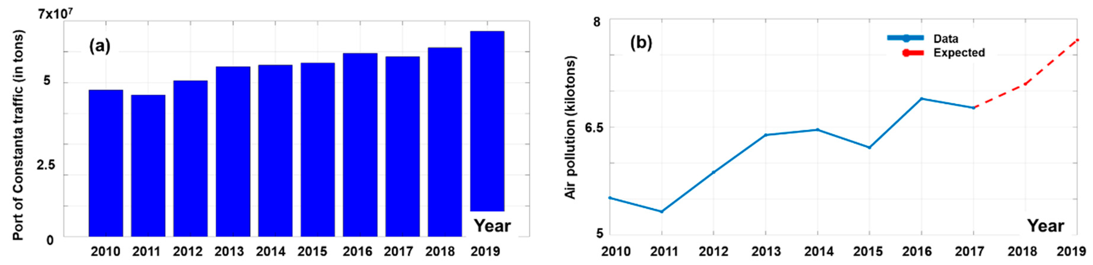
The negative environmental impact caused by ship navigation and port activities is a reality. At the same time, it is estimated that almost 50% of the entire shipping and port activities costs are associated with fuel. At this moment a 100% emission-free policy is impossible to implement, and more likely with the existing technology, a 20% to 30% reduction can be achieved [10,15]. Motivated by the fact that some important air pollutants are released only during the port activities (also known as hoteling), the idea was to investigate what it would take to develop a cold ironing project in the port of Constanta by using the local wind energy as the main supply source. In order to make such an estimation, a first step was to identify the level of air emissions from this port, the best sources of data being found in Nicolae et al. [22]. By using the traffic values and the fuel consumption reported for the port of Constanta, the authors developed a computational tool that can predict the air emissions for the two main activities: (a) ship navigation; and (b) port activities. These results were discussed in Figure 4, with the main conclusion being that air emissions are expected to escalate in the near future. The port of Constanta is a major source of pollution, but there is evidence that, in fact, some other coastal areas of the Black Sea (ex: Turkey) will be more affected [14].

The reanalysis data represents one of the best sources of wind data for the marine environment and the ones coming from the ECMWF research institute are no exception. The ERA5 is a state-of-the-art database being frequently used to assess the wind conditions from a meteorological and renewable point of view [40,41,42]. From the knowledge of the authors, at this moment there are limited (or no studies) that involve the assessment of the ERA5 wind data for the Black Sea basin, which could be considered an element of novelty. In Davy et al. 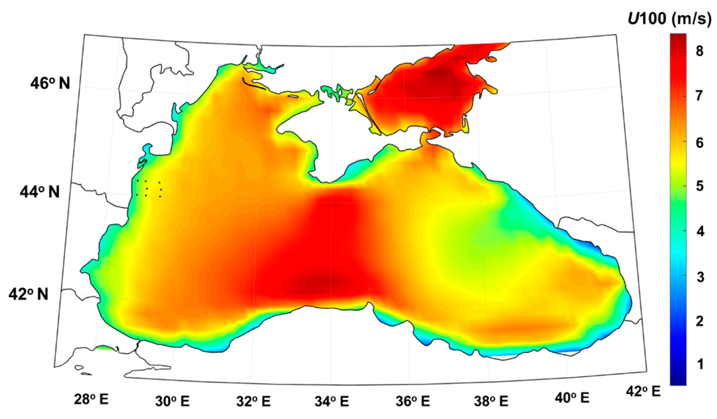[43], the ERA-Interim wind dataset (that was replaced by ERA5) was evaluated for the entire Black Sea area for the time interval located between 1979 and 2004. According to the spatial map presented in this work (U10 parameter), the best regions to develop a wind project are located in the Azov Sea and on the north-western part of the basin. In the present work, the Azov Sea is also highlighted, but in terms of the Black Sea, the best wind resources are associated with the centre part of this basin (ex: Crimea and Sinop Peninsula).

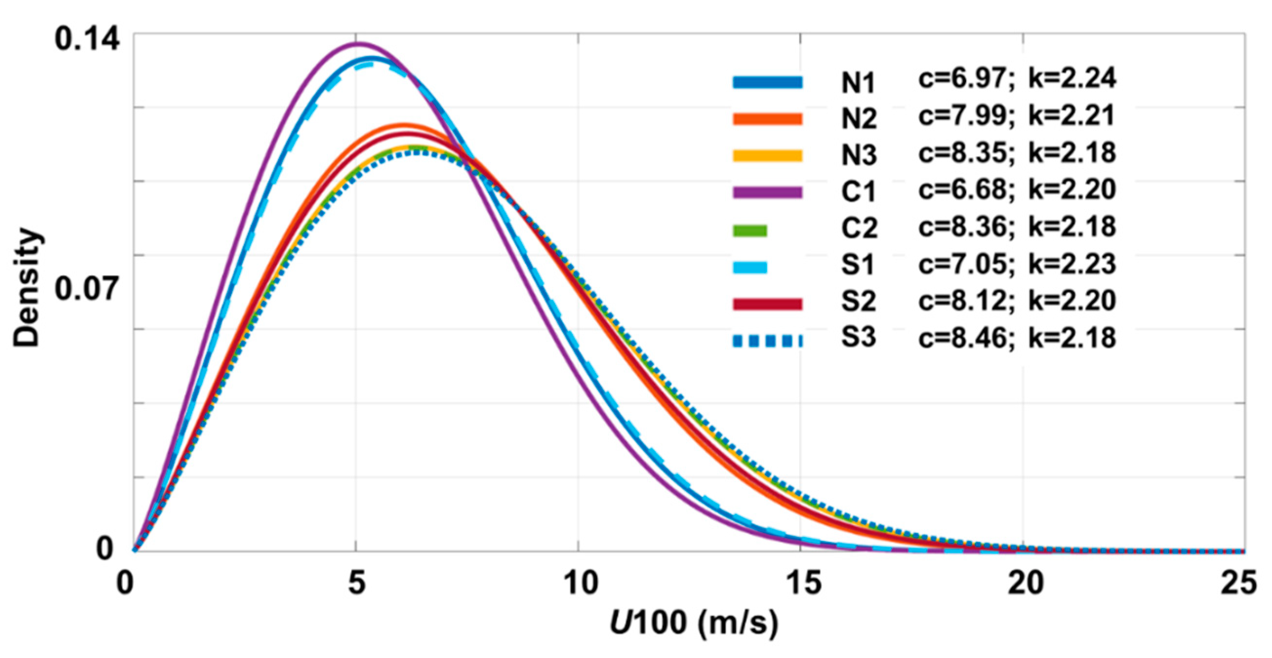
In Onea and Rusu [16], the wind conditions from the vicinity of the port of Constanta (U80; ERA-Interim) were evaluated by taking into account various distances from the shore, namely: 0, 20, 40, 60 and 80 km, respectively. For these points, the wind conditions go from 5.2 m/s (0 km) up to 6.9 m/s (60 km), values that translate to the U100 parameter are similar to 5.29 and 7.02 m/s. 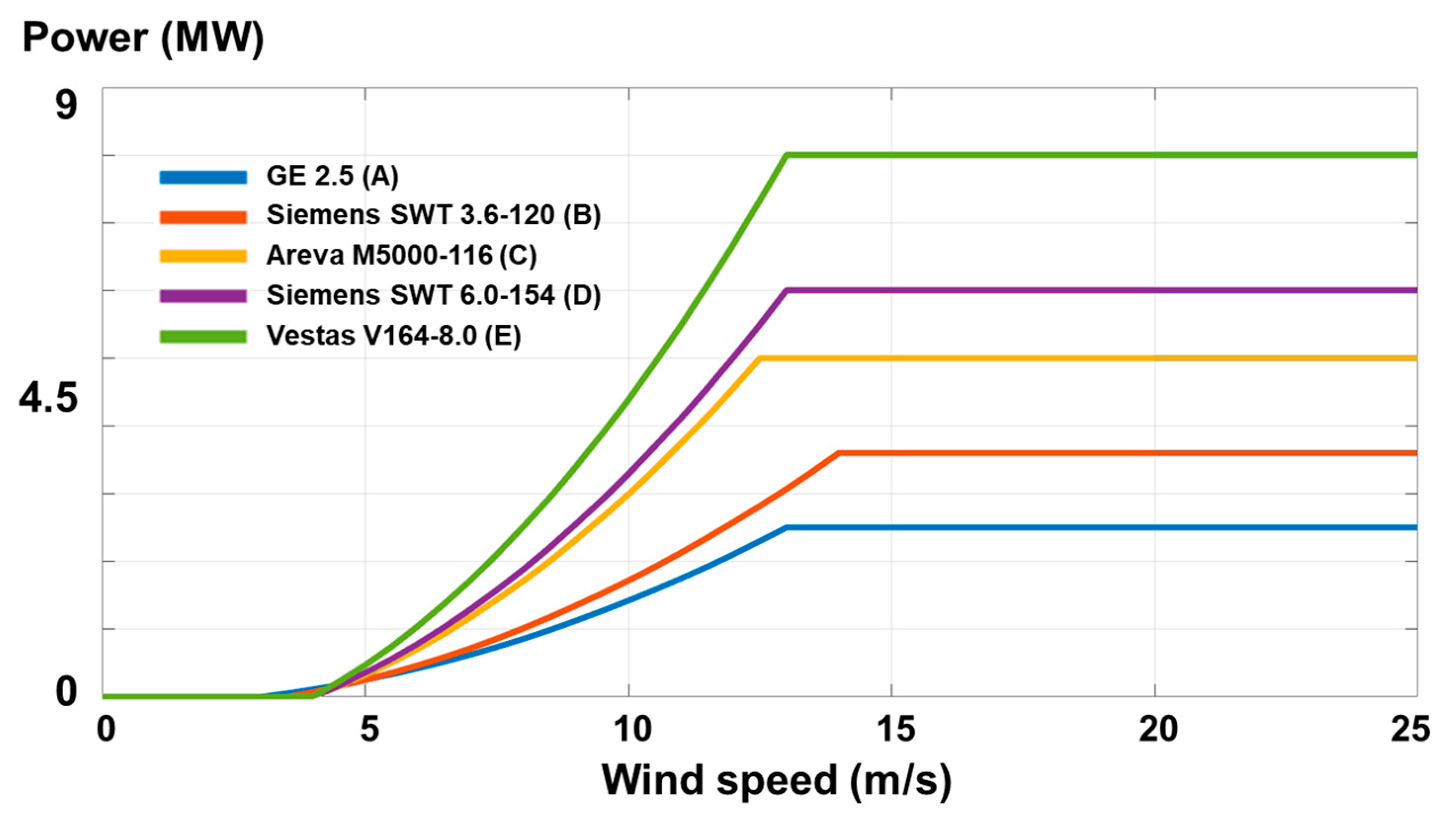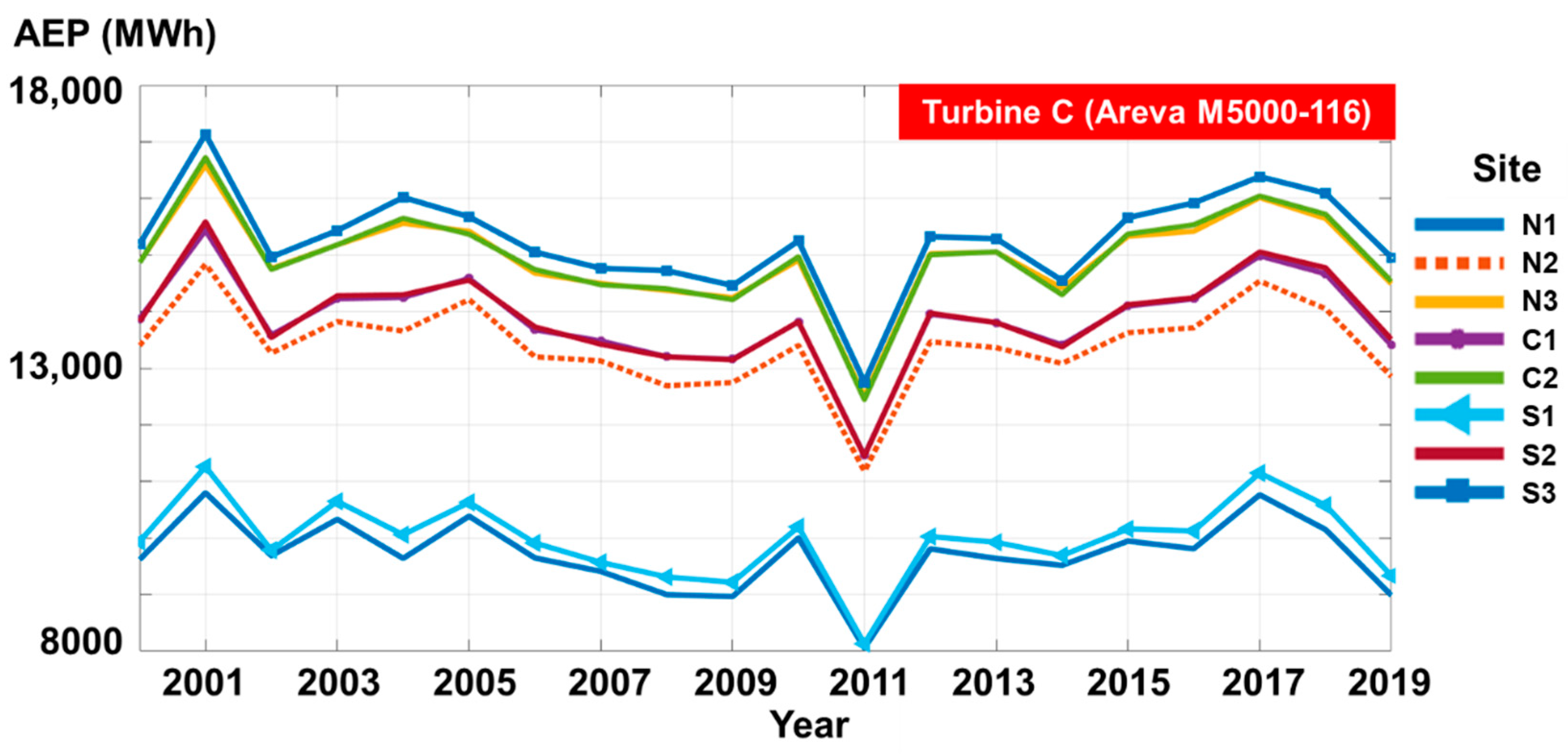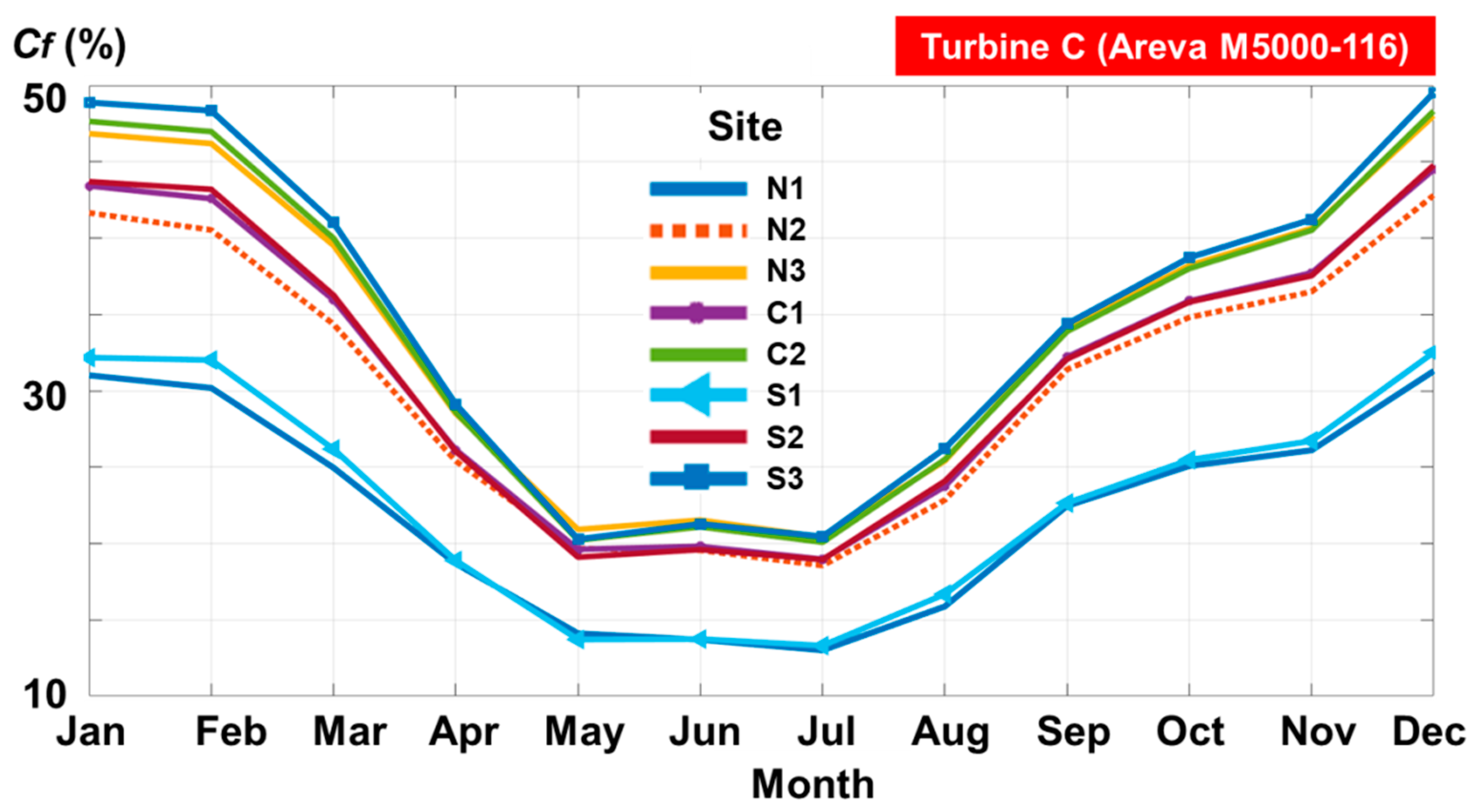From the analysis of the average values presented in Figure 6, we can notice that the Constanta site seems to reveal values that are in the same range. The Areva M5000 (Turbine C) was considered in the mentioned study, with a capacity factor that goes from 26.3% (20 km) to 29.9% (60 km), respectively. Compared to these values (that are reported at 90 m height), the present work reports values in the range of between 22.2% and 34.9%, respectively. The present paper is focused on the same target area being a continuation of Onea and Rusu [16]. Some elements of novelty and improvements that can be highlighted are: (a) ERA5 wind data was considered instead of ERA-Interim data; (b) additional wind turbines were used; (c) an estimation of the expected wind turbines required to power the port of Constanta was made by taking into account the air pollutions; (d) the expected LCOE values are indicated. The main purpose of a wind farm is to replace the pollutant emissions associated with fossil fuels consumption. By using Equation (5), it was possible to determine how many turbines will be required to cover the total emissions coming from the port activities, as it can be noticed in

Table 5. Average number of turbines estimated to cover the air pollution generated by Constanta Port activities. The results are indicated for the 20-year time interval of 2010–2019.

Site	Turbine A	Turbine B	Turbine C	Turbine D	Turbine E
N1	1741	1480	913	821	615
N2	1301	1074	660	590	442
N3	1176	962	591	527	395
C1	1260	1037	639	569	427
C2	1175	960	591	526	394
S1	1700	1442	888	799	599
S2	1258	1034	637	568	426
S3	1151	938	578	514	385

. This is a theoretical case study, since in reality, it will be impossible to cover 100% of the energy needs through natural sources, and even if this were possible at the moment there is no infrastructure or interest to implement a cold ironing project at the port of Constanta.

As expected, the number of the turbines significantly drops as we go from Turbine A to Turbine C. By looking on the current European offshore market [40] we can notice that for the marine environment the tendency is to use large scale wind turbines, so probably that Turbines A and B will no longer be considered an attractive solution. The estimated number of turbines is quite high and by looking on the largest projects (operational/under construction) we can make a comparison, namely: London Array—175 units; Hornsea 1—174 units; Gwynt y Môr—160 units; Greater Gabbard —140 units; Chenjiagang—134 units; Rampion—116 units; Anholt and Greater Changhua—111 units [44]. In the best case (Turbine E), it will take almost 2.2 farms similar to the London Array project to cover the electricity demand from Site S3.

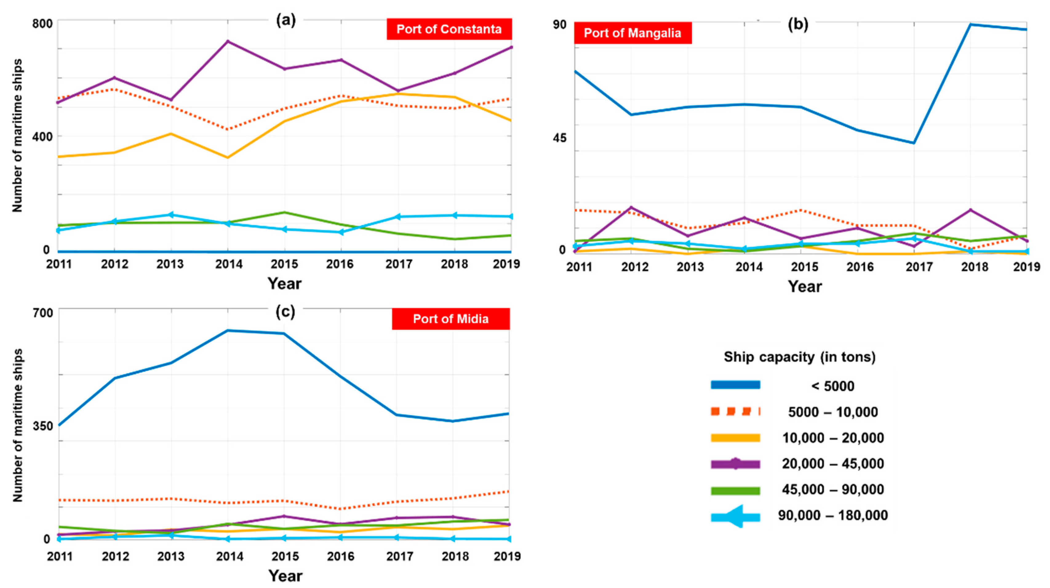
Another problem that needs to be taken into account is the number of ships that increase from year to year. In

Table 6. The enhancement in the percentage of the number of wind turbines considering as reference the emissions from the years 2010 (with the lowest values) and 2019 (with the highest values).

Site	Turbine A	Turbine B	Turbine C	Turbine D	Turbine E
N1	53.8	57.4	54.8	56.8	57.4
N2	45.9	50.3	45.7	47.5	47.3
N3	44.6	48.3	43.8	45.7	45.7
C1	44.4	48.2	44.1	45.8	45.9
C2	45	47.6	43.8	45.9	45.5
S1	52.1	55.5	52.5	54.1	54.6
S2	43.5	47.1	42.8	44.5	44.5
S3	43	46.8	42.3	44.2	43.6

is presented this dynamic, by taking into account as a base a turbine that operated in 2010 and a similar one reported for 2019. The values (in %) indicate the increase in the number of turbines required to cover the air pollution from the port of Constanta. For this 10-year interval, the values increase on average by 50%, being reported percentages in the range of: Turbine A (43–53.8%); Turbine B (46.8–57.4%); Turbine C (42.3–54.8%); Turbine D (44.2–56.8%); Turbine E (43.6–57.4%).

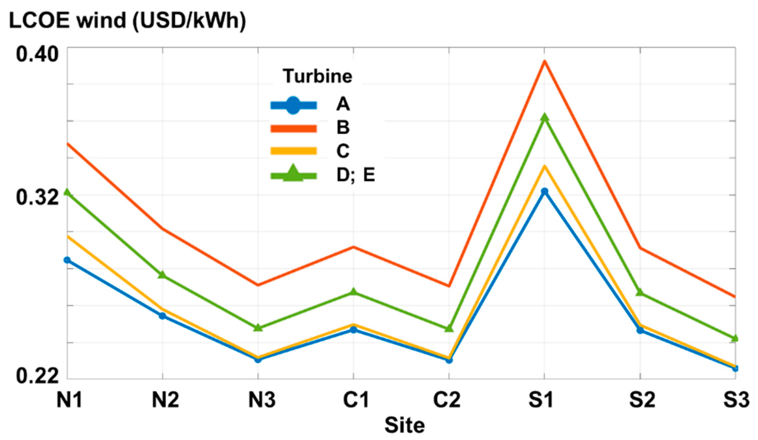
Besides the environmental aspects, the economic aspects are also important, this being revealed by the LCOE indicator. Usually a 20-year interval is required to calculate this parameter so the entire ERA5 wind data were considered (from 2000 to 2019), including the following values: CAPEX = 4500 USD/kW; OPEX = 0.048 USD/kWh; inflation = 2% per year; ageing of the systems = 1.6% per year. In the end, a cost-scaling factor was applied in order to make a difference between each site [38]. Figure 13 presents these results, from which it can be noticed that Turbines D and E reveal similar values.

According to these results, Site S1 should be avoided taking into account that it reports much higher LCOE values (range of 0.32 and 0.39 USD/kW). The most promising sites are N3, C2 and S3 where a minimum of 0.23 USD/kW may be reported in the case of Turbines A and C, respectively. From this point of view, Turbine B (Siemens SWT 3.6) reveals much lower performances, being followed by Turbines D and E, which may report a minimum of 0.25 USD/kW and a maximum of 0.36 USD/kW near Site S1. By looking on the EU expected targets [35] for the year 2025 (0.11 USD/kW) and for 2030 (0.08 USD/kW), we can notice that the minimum values reported at the Constanta sites are not even close to these indicators. This provides a rough estimation over the economic viability of an offshore wind farm that may operate in the western part of the Black Sea, this being one of the first analyses of this kind from the knowledge of the authors.

Finally, some considerations concerning the foundations will be provided at this point. This is because with the new generation of wind turbines (10 MW or greater) the offshore wind industry is already running into the problem that existing foundation types (piles) are reaching their limits in “workable size”. Obviously, the foundation type depends on the soil conditions and typically a foundation makes up to 30% of a wind turbine cost, even at 20 m depth. From this perspective, in order to implement wind farms in the target area, additional studies concerning the soil conditions and identification of the most appropriate solutions for foundation should be carried out. Additionally, an important issue in designing the foundation is represented by the current regime. This is because in the nearshore of the Black Sea, and especially in its western side, significant marine and nearshore currents are present [45,46].

5. Conclusions

In the present work, a general assessment of the wind conditions from the vicinity of the port of Constanta (Black Sea west) was carried out, by taking into account the performance of some commercial wind turbines as well. The main idea was to see how a wind farm could support a cold ironing project that may be developed in this region, taking into account that the air pollution coming from the berth activities is a reality.

First, based on the 20 years of ERA5 data, it was possible to provide a general picture of the wind conditions over the entire Black Sea area, gradually focusing on the western part and the Constanta sector. Although there are studies focused on different geographical areas, suggesting that there is no difference between onshore and nearshore wind conditions, according to these results it is clear that an offshore project will achieve better results. Apart from the performance of various wind turbines, some other important indicators were taken into account such as the CO₂ emissions and LCOE.

Going back to the original research questions, the following answers can be provided:

(a)

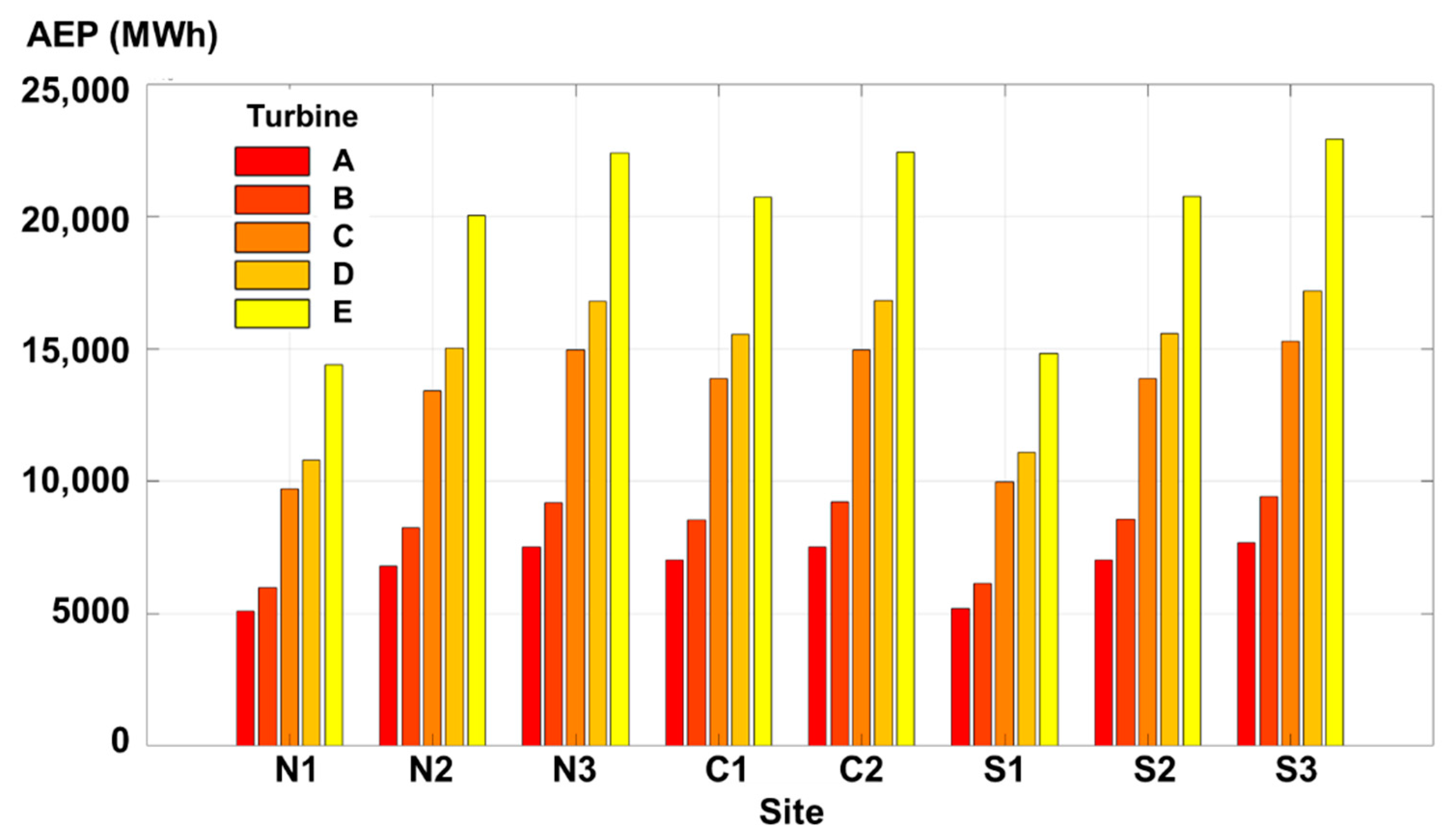
From the annual distribution of the AEP, we can definitely say that there is a significant gap between the nearshore sites (10 km) and the offshore ones exceeding 30 km. An offshore farm will be more recommended for larger projects since these can be assembled without disturbing the port of Constanta activities;

(b)

The number of turbines required to cover the electricity demand from the port of Constanta (hoteling) was estimated to be between 385 and 1741 units, depending on the site and the turbine rated capacity. Even in an optimistic scenario, it will take three or four large wind projects to cover this demand, so probably a hybrid system will be more appropriate. This is only one part of the story, because, at present, it seems that every 10 years, the electricity demand of the port of Constanta increases by at least 40%;

(c)

The best LCOE value reported for the Constanta area is close to 0.23 USD/kW, which easily exceeds the EU expectations for the near future. A renewable energy project is not a cheap solution, this being one of the reasons why most of the countries are applying a tax deduction for this type of investment. From an economical point of view, it is expected that a larger offshore project will be a better alternative to a similar one located onshore.

Looking at the current results we can mention that, in fact, the wind conditions are relatively low, this aspect is reflected by the capacity factor of the turbines (<40%) comparable to the onshore systems. Although the wind conditions are reported at 100 m height, we notice that the average wind speed can go up to 8 m/s, but even so, these conditions are below the rated wind speed of the turbines (ex: Areva M5000—12.5 m/s). This means that most of the time the wind turbines selected will not operate at full capacity, and as a consequence, the LCOE index has higher values. In order to increase the efficiency of a wind project, it will be more indicated to consider turbines defined by lower-rated speed, such as the MHI Vestas’ 10 MW turbine (Vestas, Aarhus N, Denmark) that will be defined by a rated wind speed of 10 m/s.

The cold ironing concept is emerging and slowly some major ports are taking the initiative to shift this sector to a more sustainable future. Definitely, there are a number of significant challenges that need to be overcome, including the old technological systems that need to be redesigned and the investments required to update a port infrastructure. Finally, it is difficult to predict what will happen in the future because the wind and shipping industry is evolving very fast, but certainly, a cold ironing project located on the port of Constanta will be a major gain for the entire Black Sea ecosystem.

References

1. Zhou, Y.; Daamen, W.; Velling, T.; Hoogendoorn, S. Review of maritime traffic models from vessel behavior modeling perspective. Transp. Res. Part C Emerg. Technol. 2019, 105, 323–345. [Google Scholar] [CrossRef]
2. Wang, X.; Yuen, K.F.; Wong, Y.D.; Li, K.X. How can the maritime industry meet Sustainable Development Goals? An analysis of sustainability reports from the social entrepreneurship perspective. Transp. Res. Part D Transp. Environ. 2020, 78, 102173. [Google Scholar] [CrossRef]
3. Toscano, D.; Murena, F. Atmospheric ship emissions in ports: A review. Correlation with data of ship traffic. Atmos. Environ. X 2019, 4, 100050. [Google Scholar] [CrossRef]
4. Wan, Z.; Zhang, Q.; Xu, Z.; Chen, J.; Wang, Q. Impact of emission control areas on atmospheric pollutant emissions from major ocean-going ships entering the Shanghai Port, China. Mar. Pollut. Bull. 2019, 142, 525–532. [Google Scholar] [CrossRef]
5. Murena, F.; Mocerino, L.; Quaranta, F.; Toscano, D. Impact on air quality of cruise ship emissions in Naples, Italy. Atmos. Environ. 2018, 187, 70–83. [Google Scholar] [CrossRef]
6. Mousavi, A.; Sowlat, M.H.; Hasheminassab, S.; Pikelnaya, O.; Polidori, A.; Ban-Weiss, G.; Sioutas, C. Impact of particulate matter (PM) emissions from ships, locomotives, and freeways in the communities near the ports of Los Angeles (POLA) and Long Beach (POLB) on the air quality in the Los Angeles county. Atmos. Environ. 2018, 195, 159–169. [Google Scholar] [CrossRef]
7. Styhre, L.; Winnes, H.; Black, J.; Lee, J.; Le-Griffin, H. Greenhouse gas emissions from ships in ports—Case studies in four continents. Transp. Res. Part D Transp. Environ. 2017, 54, 212–224. [Google Scholar] [CrossRef]
8. Gutierrez-Romero, J.E.; Esteve-Perez, J.; Zamora, B. Implementing Onshore Power Supply from renewable energy sources for requirements of ships at berth. Appl. Energy 2019, 255, 113883. [Google Scholar] [CrossRef]
9. Zis, T.P.V. Prospects of cold ironing as an emissions reduction option. Transp. Res. Part A Policy Pract. 2019, 119, 82–95. [Google Scholar] [CrossRef] [Green Version]
10. Iris, C.; Lam, J.S.L. A review of energy efficiency in ports: Operational strategies, technologies and energy management systems. Renew. Sustain. Energy Rev. 2019, 112, 170–182. [Google Scholar] [CrossRef]
11. Energy Transition in Hamburgs Port—Hamburg Marketing. Available online: https://marketing.hamburg.de/energy-transition-in-hamburgs-port.html (accessed on 15 June 2020).
12. Kotrikla, A.M.; Lilas, T.; Nikitakos, N. Abatement of air pollution at an aegean island port utilizing shore side electricity and renewable energy. Mar. Policy 2017, 75, 238–248. [Google Scholar] [CrossRef]
13. Wang, W.; Peng, Y.; Li, X.; Qi, Q.; Feng, P.; Zhang, Y. A two-stage framework for the optimal design of a hybrid renewable energy system for port application. Ocean Eng. 2019, 191, 106555. [Google Scholar] [CrossRef]
14. Gryning, S.-E.; Batchvarova, E. Air Pollution Modeling and Its Application XIII; Springer Science & Business Media: Berlin/Heidelberg, Germany, 2012; ISBN 978-1-4615-4153-0. [Google Scholar]
15. Rata, V.; Rusu, E. Can air quality be influenced in coastal areas by shipping? J. Mar. Sci. 2019, 2. [Google Scholar] [CrossRef]
16. Onea, F.; Rusu, L. A study on the wind energy potential in the romanian coastal environment. J. Mar. Sci. Eng. 2019, 7, 142. [Google Scholar] [CrossRef] [Green Version]
17. Rusu, L.; Raileanu, A.B.; Onea, F. A comparative analysis of the wind and wave climate in the black sea along the shipping routes. Water 2018, 10, 924. [Google Scholar] [CrossRef] [Green Version]
18. Offshore Wind in Europe—Key Trends and Statistics 2019|WindEurope. Available online: https://windeurope.org/about-wind/statistics/offshore/european-offshore-wind-industry-key-trends-statistics-2019/ (accessed on 17 June 2020).
19. Bathymetric Data Viewer. Available online: https://maps.ngdc.noaa.gov/viewers/bathymetry/ (accessed on 31 May 2019).
20. Black Sea Ship Traffic|Ship Traffic. Available online: http://www.shiptraffic.net/2001/04/black-sea-ship-traffic.html (accessed on 17 July 2020).
21. Portul Constanta. Available online: https://www.portofconstantza.com/pn/page/np_statistici_port (accessed on 18 June 2020).
22. Nicolae, F.; Roman, I.; Cotorcea, A. Air pollution from the maritime transport in the romanian black sea coast. Rev. Cercet. Mar. Rev. Rech. Mar. Mar. Res. J. 2017, 47, 260–266. [Google Scholar]
23. What Are the Changes from ERA-Interim to ERA5?—Copernicus Knowledge Base—ECMWF Confluence Wiki. Available online: https://confluence.ecmwf.int//pages/viewpage.action?pageId=74764925 (accessed on 18 June 2020).
24. Hersbach, H.; Bell, B.; Berrisford, P.; Hirahara, S.; Horányi, A.; Muñoz-Sabater, J.; Nicolas, J.; Peubey, C.; Radu, R.; Schepers, D.; et al. The ERA5 global reanalysis. Q. J. R. Meteorol. Soc. 2020. [Google Scholar] [CrossRef]
25. Onea, F.; Rusu, L. Evaluation of some state-of-the-art wind technologies in the nearshore of the black sea. Energies 2018, 11, 2452. [Google Scholar] [CrossRef] [Green Version]
26. Onea, F.; Ciortan, S.; Rusu, E. Assessment of the potential for developing combined wind-wave projects in the European nearshore. Energy Environ. 2017, 28, 580–597. [Google Scholar] [CrossRef]
27. Does Downloading Data at Higher Resolution Improve the Output—Copernicus Knowledge Base—ECMWF Confluence Wiki. Available online: https://confluence.ecmwf.int/display/CKB/Does+downloading+data+at+higher+resolution+improve+the+output (accessed on 18 June 2020).
28. Archer, C.L.; Jacobson, M.Z. Evaluation of global wind power. J. Geophys. Res. Atmos. 2005, 110. [Google Scholar] [CrossRef] [Green Version]
29. Rusu, E.; Onea, F. Joint evaluation of the wave and offshore wind energy resources in the developing countries. Energies 2017, 10, 1866. [Google Scholar] [CrossRef] [Green Version]
30. Elsner, P.; Suarez, S. Renewable energy from the high seas: Geo-spatial modelling of resource potential and legal implications for developing offshore wind projects beyond the national jurisdiction of coastal States. Energy Policy 2019, 128, 919–929. [Google Scholar] [CrossRef]
31. Elsner, P. Continental-scale assessment of the African offshore wind energy potential: Spatial analysis of an under-appreciated renewable energy resource. Renew. Sustain. Energy Rev. 2019, 104, 394–407. [Google Scholar] [CrossRef] [Green Version]
32. de Assis Tavares, L.F.; Shadman, M.; de Assad, L.P.F.; Silva, C.; Landau, L.; Estefen, S.F. Assessment of the offshore wind technical potential for the Brazilian Southeast and South regions. Energy 2020, 196, 117097. [Google Scholar] [CrossRef]
33. Onea, F.; Rusu, E. Sustainability of the reanalysis databases in predicting the wind and wave power along the european coasts. Sustainability 2018, 10, 193. [Google Scholar] [CrossRef] [Green Version]
34. Salvacao, N.; Soares, C.G. Wind resource assessment offshore the Atlantic Iberian coast with the WRF model. Energy 2018, 145, 276–287. [Google Scholar] [CrossRef]
35. Rusu, E.; Onea, F. An assessment of the wind and wave power potential in the island environment. Energy 2019, 175, 830–846. [Google Scholar] [CrossRef]
36. Al-Nassar, W.K.; Neelamani, S.; Al-Salem, K.A.; Al-Dashti, H.A. Feasibility of offshore wind energy as an alternative source for the state of Kuwait. Energy 2019, 169, 783–796. [Google Scholar] [CrossRef]
37. Quitoras, M.R.D.; Abundo, M.L.S.; Danao, L.A.M. A techno-economic assessment of wave energy resources in the Philippines. Renew. Sustain. Energy Rev. 2018, 88, 68–81. [Google Scholar] [CrossRef]
38. Jacobsen, H.K.; Hevia-Koch, P.; Wolter, C. Nearshore and offshore wind development: Costs and competitive advantage exemplified by nearshore wind in Denmark. Energy Sustain. Dev. 2019, 50, 91–100. [Google Scholar] [CrossRef]
39. US EPA. Greenhouse Gases Equivalencies Calculator-Calculations and References. Available online: https://www.epa.gov/energy/greenhouse-gases-equivalencies-calculator-calculations-and-references (accessed on 4 January 2019).
40. Esteban, M.D.; López-Gutiérrez, J.-S.; Valdecantos, V.N. Offshore Wind Farms; MDPI: Basel, Switzerland, 2020; ISBN 978-3-03928-562-4. [Google Scholar]
41. Olauson, J. ERA5: The new champion of wind power modelling? Renew. Energy 2018, 126, 322–331. [Google Scholar] [CrossRef] [Green Version]
42. Shepherd, T.J.; Barthelmie, R.J.; Pryor, S.C. Sensitivity of wind turbine array downstream effects to the parameterization used in WRF. J. Appl. Meteorol. Climatol. 2020, 59, 333–361. [Google Scholar] [CrossRef]
43. Davy, R.; Gnatiuk, N.; Pettersson, L.; Bobylev, L. Climate change impacts on wind energy potential in the European domain with a focus on the Black Sea. Renew. Sustain. Energy Rev. 2018, 81, 1652–1659. [Google Scholar] [CrossRef] [Green Version]
44. List of Offshore Wind Farms—Wikipedia. Available online: https://en.wikipedia.org/wiki/List_of_offshore_wind_farms (accessed on 22 June 2020).
45. Rusu, E.; Macuta, S. Numerical modelling of longshore currents in marine environment. Environ. Eng. Manag. J. 2009, 8, 147–151. [Google Scholar] [CrossRef]
46. Rusu, E. Modelling of wave–current interactions at the mouths of the Danube. J. Mar. Sci. Technol. 2010, 15, 143–159. [Google Scholar] [CrossRef]
Figure 1. Constanta nearshore and the reference sites considered for evaluation. The red points are used to highlight the roadstead sector of Constanta harbour. Figure processed from Google Earth (2020).
Jmse 08 00550 g001
Figure 2. Location of the reference points and the port of Constanta activities reported for the time frame 17/07/2020 16:30 h. Results processed from Black Sea ship traffic [20].
Jmse 08 00550 g002
Figure 3. Number of maritime ships reported for the main Romanian ports. The results include different ships capacities, being reported for: (a) Port of Constanta; (b) Port of Mangalia; (c) Port of Midia. Data processed from [21].
Jmse 08 00550 g003
Figure 4. Port of Constanta statistics corresponding to the 20-year time interval of 2010–2019, where: (a) overall ship traffic—in tonnes; (b) air pollution (nitrogen oxides (NOx), Particular Matter (PM) and Volatile Organic Compounds (VOCs) in kilotons considering only the port activities. The air pollution associated with the years 2017, 2018 and 2019 were estimated from the existing data [21,22].
Jmse 08 00550 g004
Figure 5. Power curves of the turbines considered for evaluation.
Jmse 08 00550 g005
Figure 6. The spatial distribution of the U100 (m/s) parameter over the Black Sea area. Results computed for the 20-year time interval of 2000–2019.
Jmse 08 00550 g006
Figure 7. The spatial differences (in %) between the total time data and the main seasons. Results for the U100 parameter (average values) considering the 20-year time interval of ERA5 data, where: (a) spring; (b) summer; (c) autumn; (d) winter.
Jmse 08 00550 g007
Figure 8. Weibull PDF (probability density function) distributions indicated for all the reference sites, considering the ERA5 wind data for the 20-year time interval of 2000–2019.
Jmse 08 00550 g008
Figure 9. The monthly wind roses associated with Site C1, expressed in terms of the wind classes (C1–C7). Results reported for the 20-year time interval of 2000–2019.
Jmse 08 00550 g009
Figure 10. Annual electricity production (MWh) corresponding to the full time distribution.
Jmse 08 00550 g010
Figure 11. Annual distribution of the Annual Electricity Production (AEP) values associated with Turbine C (Areva M5000-116).
Jmse 08 00550 g011
Figure 12. Capacity factor—monthly distribution associated with Turbine C (Areva M5000-116).
Jmse 08 00550 g012
Figure 13. Levelized Cost of Energy (LCOE) estimated in the reference sites for all the wind turbines considered (A, B, C, D and E).
Jmse 08 00550 g013