Measuring Community Disaster Resilience in the Conterminous Coastal United States


Department of Geosciences, Florida Atlantic University, Boca Raton, FL 33431, USA
*
Author to whom correspondence should be addressed.
ISPRS Int. J. Geo-Inf. 2020, 9(8), 469; https://doi.org/10.3390/ijgi9080469
Submission received: 27 June 2020
/
Revised: 20 July 2020
/
Accepted: 21 July 2020
/
Published: 23 July 2020
(This article belongs to the Special Issue Geomatic Applications to Coastal Research: Challenges and New Developments)
Abstract
:In recent years, building resilient communities to disasters has become one of the core objectives in the field of disaster management globally. Despite being frequently targeted and severely impacted by disasters, the geographical extent in studying disaster resilience of the coastal communities of the United States (US) has been limited. In this study, we developed a composite community disaster resilience index (CCDRI) for the coastal communities of the conterminous US that considers different dimensions of disaster resilience. The resilience variables used to construct the CCDRI were justified by examining their influence on disaster losses using ordinary least squares (OLS) and geographically weighted regression (GWR) models. Results suggest that the CCDRI score ranges from −12.73 (least resilient) to 8.69 (most resilient), and northeastern communities are comparatively more resilient than southeastern communities in the study area. Additionally, resilience components used in this study have statistically significant impact on minimizing disaster losses. The GWR model performs much better in explaining the variances while regressing the disaster property damage against the resilience components (explains 72% variance) than the OLS (explains 32% variance) suggesting that spatial variations of resilience components should be accounted for an effective disaster management program. Moreover, findings from this study could provide local emergency managers and decision-makers with unique insights for enhancing overall community resilience to disasters and minimizing disaster impacts in the study area.
1. Introduction
Natural hazards are considered as one of the biggest challenges of the 21st century around the globe. Disasters have increased both in frequency and severity over the last few decades, causing unparalleled damage to properties and loss of human lives [1,2,3]. Communities in the coastal areas are particularly vulnerable to natural hazards that are concentrated along the coast [4,5]. With the increasing population in the coastal areas along with the projected coastal hazards with more intensity [6,7,8], coastal communities are under great threat from natural hazards now more than ever. Global climate change, as well as increased human activities such as rapid urbanization and population growth, act as drivers of natural hazard impacts; especially in the coastal regions. The coastal communities in the United States (US) are vulnerable to and frequently impacted by coastal hazards including both rapid-moving disasters such as tropical cyclones and storm surges, and comparatively slow-moving disasters such as sea level rise, land subsidence, etc. However, disaster impacts are not even across the coastal US as disaster response and recovery varies across the coastal communities which might be related to the varying nature of hazard exposure, hazard impacts, and socio-economic and environmental aptitudes of the communities [9,10,11,12,13]. Hence, identifying the principal factors that make these communities less vulnerable and more resilient to coastal hazards is extremely important for disaster preparedness and mitigation.
There are quite a few studies that developed conceptual models in order to define and measure disaster resilience [14,15,16,17,18,19,20,21]. Despite these vast studies, there is still no consensus among the researchers about the definition of disaster resilience and how to measure it [17,22,23]. However, two things were found common in the definition of resilience to disasters: vulnerability and adaptive capacity. While some researchers defined resilience as part of adaptive capacity [16,24,25], others perceived it associated with vulnerability [17,22,23]. Connections of resilience with both vulnerability and adaptive capacity have also been studied [26,27]. Adaptive capacities showing resilience to disasters correspond to a community’s strengths or weaknesses to cope with disaster impacts [15,25]. Adaptive capacities in resilience studies can be measured based on a community’s socio-economic, infrastructural, ecological, environmental, and institutional capacities. According to Intergovernmental Panel on Climate Change (IPCC), vulnerability is defined as a function of exposure, sensitivity, and adaptive capacity [28]. Disaster resilience is often seen as negatively related with vulnerability and positively connected with adaptive capacities of a community [26]. After reviewing these literatures and conceptual models of disaster resilience, we consider disaster resilience as diverse but associated with adaptive capacity and vulnerability in this paper.
Like the definition of disaster resilience, there are considerable differences among the researchers when it comes to measure disaster resilience of communities. Discrepancy in the definition of resilience does not make it any easier. Community disaster resilience corresponds to the ability of a community to cope with disasters by reducing the vulnerabilities. Therefore, highly resilient communities are less vulnerable to disasters and can cope with disasters better [22,29]. Disaster resilience of communities is generally quantified or measured by creating resilience index and models based on different dimensions or indicators of community resilience such as social, economic, environmental, community capital, human, etc. There are a number of studies that developed different models and indices in the field of community disaster resilience and vulnerability [10,12,14,19,30,31,32,33]. Among them, studies that are most relevant to this research are discussed as follows. The social vulnerability index, created by Cutter and her team, was constructed using 42 socioeconomic variables based on previous studies for the entire US [30]. Principal component analysis (PCA) was used to reduce the variables to 11 components which accounted for almost 76% of the variance. Then the component scores were added together for each county to create the index scores. The authors tried to validate their index by correlating the index scores with presidential disaster declarations and found no correlation. However, the approach taken by the researchers helped to understand the necessity of statistical modeling to create and validate the index. Coastal Resilience Index (CRI), constructed by National Oceanic and Atmospheric Administration (NOAA) uses six components including critical facilities, transportation, community plans, mitigation measures, business plan, and social system to create the index that mainly concentrates on coastal hazards [33]. The Baseline Resilience Indicators for Communities (BRIC) is another pioneer work by Cutter and her team [23] that considers six components of disaster resilience including social, economic, infrastructural, institutional, community, and environmental to measure community disaster resilience. Each of the six components include several variables that were selected based on previous studies. The component scores were added together to construct the composite resilience index and is applicable in a policy context. Sherrieb and colleagues [19] selected 88 variables that represent disaster resilience. After the multicollinearity check, 17 variables were retained that represent two components of disaster resilience including social capital and economic development that measure community resilience. These studies used different sets of resilience indicators to model and measure disaster resilience of communities. However, quantitative validation of the resilience index and the variables used to create the resilience index has hardly been conducted and remain a severe limitation in this field [34,35].
Community resilience to disasters has been measured by creating an index using the resilience indicators in previous studies. However, the relationships (spatial and non-spatial) between disaster resilience indicators and impacts of disasters on real-life have rarely been studied. Additionally, exploring the spatial distribution of disaster resilience and how the relationships between disaster resilience indicators and impacts from disasters vary spatially could help local communities to customize area-specific disaster management plan. To overcome these gaps in this field, this study evolves around two broad research questions: (1) does the disaster resilience vary across the coastal communities in the US, and if so, is there any spatial pattern of disaster resilience? and (2) is there any spatial or non-spatial relationship between indicators of disaster resilience and losses due to disasters in the coastal US? According to the US Census Bureau, the coastline of the entire US is more than 12,000 miles long. Therefore, how disaster resilience varies from one place to another within a large geographic area such as coastal US should be explored and could reveal important information regarding overall disaster management in this region.
In this study, we first created a composite community disaster resilience index (CCDRI) based on resilience variables from different dimensions of resilience using commonly practiced mathematical and statistical procedures. Then we examined the relationship between the variables used to create the CCDRI and disaster losses sustained by the coastal communities to see how resilience variables influence disaster losses such as property damage in this area.
2. Materials and Methods
2.1. Study Area
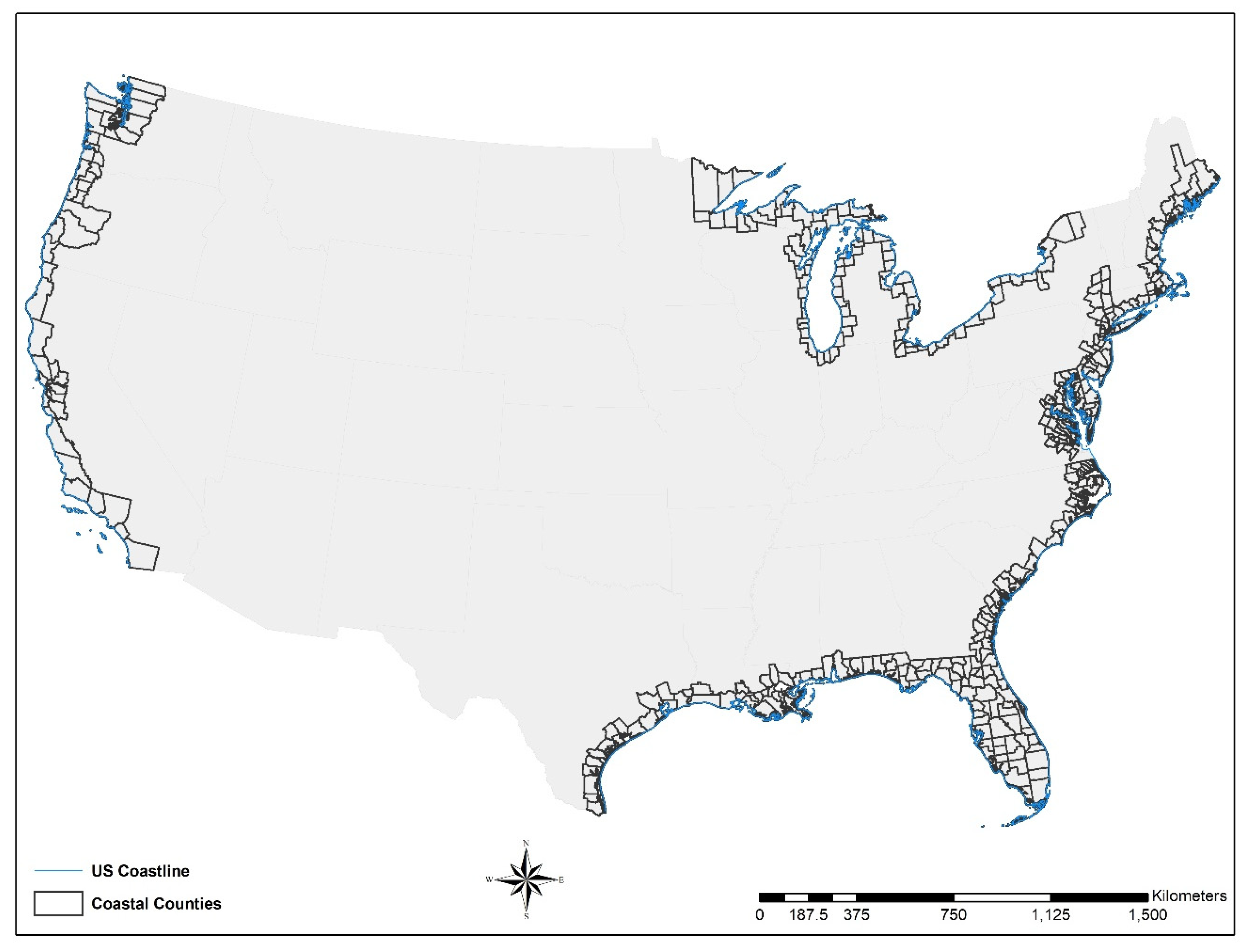
This study focuses on the coastal counties of the conterminous US where each county is considered as a ‘community’. According to the Coastal Zone Management Program (CZMP), which is a partnership between the US federal government and the coastal and Great Lake states and territories accredited by the Coastal Zone Management Act of 1972 [36], there were 414 coastal territories in the conterminous US in 2009, and among them 397 are counties. These 397 counties were selected as the study area which are considered as ‘communities’ in this research (Figure 1). The terms ‘community’ and ‘county’ are used interchangeably in this study. These counties are adjacent to the Atlantic and Pacific Ocean as well as to the five Great Lakes of the US. There are vast differences in geographic, atmospheric, and environmental attributes in these coastal counties. For example, the highest average elevation of a community is 923 meters (Whatcom County, Washington) and the lowest average elevation is 1.82 meters (Plaquemines Parish, Louisiana) in the study area. The average elevation of all these counties is 125.9 meters. Additionally, according to the US Census Bureau, Los Angeles County, California is the most populous county with a population over 9.81 million in 2010. On the other hand, the lowest population was recorded in Kenedy County, Texas which had only 416 people living there in 2010. Average household median income was found as $51,829.03 in 2010 in these coastal counties. However, the highest household median income was in Fairfax County, Virginia ($105,416) and the lowest household income ($22,881) was found in Willacy County, Texas. These differences are also reflected when it comes to property damage caused by coastal hazards. There was over $4.6 billion of property damage caused by flooding events only between 2001–2010 in these coastal counties. Cook County, Illinois sustained highest property damage caused by flooding in those 10-years period (over $369.5 million in total) where a total of 61 counties had no property damage caused by floods.
2.2. Data
Data for this research were collected from 9 different data sources (Table 1). As mentioned earlier, this research focuses on the year 2010 for constructing and analyzing the composite resilience indicator, 2010 decennial census is the mostly used dataset. However, data were not always available for all the resilience variables for the year 2010 (Table 1). For those variables where data were not available for the year 2010, data were acquired for the closest year possible to 2010. For example, we used National Land Cover Dataset (NLCD) for the year 2011 for the variable named percent of wetlands as 2011 is the closest year to 2010.
After collecting the data for the variables, the raw datasets were normalized by transforming the datasets into percentages, rates, and averages. Normalization of the datasets were carried out in a way so that communities with different sizes and characteristics can be compared [10]. After the necessary data transformation and normalization, the direction of each variable was adjusted so that larger values resemble to higher resilience. In doing this, some variable values were inverted [37].
2.3. Dimensions of the CCDRI
Generally, an index is created by combining different sets of variables or indicators using mathematical and statistical methods. While variables cannot directly measure a phenomenon individually, a composed index created by combining those variables could be effective for decision-making and temporal comparison of a phenomenon. A wide range of variables have been used by researchers in their attempts to measure community disaster resilience. These variables represent different dimensions of resilience including social, economic, community competence, human, environmental, infrastructural, physical, ecological, and institutional resilience [10,19,22,38,39,40]. Based on previous studies, a total set of 44 variables were initially selected that represent five dimensions of community disaster resilience in this study: social, economic, community engagement and Capital, housing/infrastructural, and environmental resilience. A multicollinearity analysis was conducted among those initial set of variables and a few variables were eliminated because they showed high degree of multicollinearity. After the elimination, 25 variables were selected for further analysis.
As mentioned above, variables were selected from five different dimensions of disaster resilience based on previous studies. Table 2 illustrates the description of the final sets of 25 variables, their respective resilience dimension, and the data sources for those variables. Table 2 also shows the previous studies that used those variables to measure disaster resilience as a means of justification behind inclusion of those variables in this study. Each of the five resilience dimensions have five variables.
The variables in the social dimension include the demographic characteristics of a community in terms of gender, physical well-being, and effective communication before, during, and after a disaster event. For example, it is our expectation that a community that has a larger number of physicians and health insurance enrollments will demonstrate a higher level of disaster resilience than the communities that do not have these characteristics. Similarly, communities with more access to telephone services and personal vehicles will be better prepared for and will respond better before and during a disaster. Having these characteristics corresponds to effective communications of a community during an emergency which enhances disaster resilience of that community. Additionally, women are considered more vulnerable than men during disasters and having less female population corresponds to higher disaster resilience in a community [40].
Communities with strong economic and financial resources as well as economic equality across different ethnic, racial, and gender groups correspond to faster recovery and greater resilience [23,25]. Therefore, variables in the economic dimension of this study include economic equality as well as the ability to financial resource generation of a community. Gini coefficient measures the income distribution equality among different races and ethnicities [23]. We inverted the values of Gini coefficients so that more equality means more resilient. We have also included gender income equality by adding the inverted absolute difference between male and female median income. Communities with equal wage policy are more resilient to disasters [23]. Additionally, the ability to more economic resource generation of communities shows better preparedness during disasters and those communities tend to recover faster from the impacts of disasters. Therefore, communities with large percentages of employed workforce and federal government employee pose more disaster resilience. Furthermore, employees in the temporary employment sector like farming, fisheries, forestry, extractive industry (e.g.: mining), or tourism industry are more vulnerable to disasters [23].
Community engagement/involvement as well as community capital are important aspects of overall community resilience [15,49]. While communities with higher social capitals tend to recover faster from disaster impacts [15], higher levels of community engagement and civic involvement enhances communities’ ability to cope with before and during disasters [23]; thus making communities more disaster resilient. People living in the same community for longer period demonstrates a more engaged and involved attitude towards the community who are more likely to come forward in helping the community inhabitants in their time of need. Additionally, communities that have higher percentages of population affiliated with local/religious organizations are more than like to have some sort of social capital to go to for help except their families and neighbors. Furthermore, we included the per capita financial revenue generation of local governments in the community capital dimension of this study. The idea is that local governments with higher financial revenue generation will have more resources available to help the local community with disaster preparedness and recovery and will not have to wait for federal assistance.
The variables in the housing/infrastructure dimension include the building materials and quality of housing construction as well as infrastructure capacity of communities for temporary shelters, emergency evacuation, medical care, and strengths of the infrastructures. For example, mobile homes are extremely vulnerable to coastal hazards like tropical cyclones. Similarly, housing units that are more recently built are more likely to stand out during disasters compared to older constructions. Communities with larger length of roads can plan better for an emergency evacuation while larger number of vacant houses that are for rent could be helpful for temporary shelters during disasters. Additionally, communities with more hospital beds could better serve with medical care to the injured and thus reduce the disaster fatalities.
The environmental dimension is another important aspect of disaster resilience. The variables in this dimension include the percentage of wetlands that can act as a natural flood buffer during a storm surge or flooding event and demonstrates environmental quality of communities that increase absorptive capacity [23]. Another important variable of this dimension is the average elevation of the communities. In coastal areas like this study, elevation could play a very important role in preventing tropical cyclone induced flooding and storm surge and resulting property damage and human life loss [50]. The percentage of urban area was also included as one of the variables reflecting environmental resilience. The urban area tends to show higher disaster resilience compared to the rural areas as found in the previous study [51] and has been used by previous researchers as a resilient variable in the disaster study [47]. We also included inverted hazard exposure as a variable of environmental resilience. As mentioned earlier, exposure is considered as a very important function to measure disaster vulnerability along with sensitivity and adaptive capacity [3]. Furthermore, the level of hazard exposure helps to improve pre-disaster planning as well as post-disaster recovery of communities. Since exposures to natural hazards are often related to geophysical conditions of a community, we included inverted hazard exposure value as a variable of environmental resilience. We hypothesize that less exposure to hazards mirrors more resilient community. In this study, the hazard exposure was calculated by a weighted method originally developed by Lam et al. (2016) [44] other than simply using number of hazard events as the exposure. For example, Hurricane Katrina caused enormous damage to some coastal communities and was one of the costliest disasters in the US history. Naturally, an event like Hurricane Katrina carries more weight than other hazard events that caused little to no damage in the study area. Five major types of coastal hazards were considered in this study including hurricane, flood, coastal (includes storm surge and coastal flooding), thunderstorm, and tornado. The hazard damage and event data were obtained from the NCEI storm database. Following Lam et al. (2016) [44], hazard exposure was calculated using the below equation:
where = weight of a hazard type ; = number of hazard type occurred in the county ; and = difference between begin and end dates of hazard event of type . The weight of a hazard type was calculated using the below equation:
where = total damage of hazard type and = total damage of all hazards. Therefore, for each of the five hazard types, we got a hazard exposure value. Then all the five exposure values were added together to get the total exposure value of each county.
2.4. Constructing the CCDRI
Community disaster resilience is a multidimensional concept [40] that includes five dimensions of disaster resilience comprising social, economic, community engagement and capital, housing/infrastructural, and environmental resilience in this study. To measure and compare the composite community disaster resilience across our study area, we constructed an index (CCDRI). In doing this, PCA with varimax rotation was used in SPSS (version 26) to reduce the number of variables from the list of 25 variables across five resilience dimensions firstly. After examining the PCA results, eight components with eigenvalues greater than 1.0 from the previously mentioned five dimensions were extracted to quantify the community disaster resilience by producing the factor scores. Table 3 shows the dominant variables and their respective resilience dimensions of the eight components that explains 69.7% of the variance in the data. Interestingly, these components were characterized by variables from multiple dimensions, and therefore, created inter-dimensional components of disaster resilience. For example, the first component is dominated by three variables (local government finances, revenue per capita, total length of roads per sq. km., and percent of urban area) from three different resilience dimensions, and we named it based on the dimensions that each of those variables represent (Table 3).
Then the eight multidimensional components were combined into a single measure to create the CCDRI. In doing this, an additive model was used to construct the overall CCDRI for the study area. Since there is still an absence of a recognized method to assign weights to the components [40], an additive model is the best option to combine multidimensional components into a singular value [30]. Additionally, since the directions of the variables suggest that higher value means more resilient, high CCDRI score corresponds to more resilient community. Furthermore, we assumed that each component was equally important and carries equal weight to the overall CCDRI in the study area.
2.5. Data Analyses
After calculating the CCDRI, we extended our analyses by investigating the spatial distribution of CCDRI to examine the high and less resilient communities in our study area. Then we utilized Local Index of Spatial Autocorrelation (LISA) in ArcGIS to assess the statistically significant hot spots, cold spots, and spatial outliers by calculating the local Moran’s I statistic for CCDRI scores and eight resilience components from PCA analysis. The hot spots are displayed by high-high clusters where the cold spots are shown by low-low clusters. The high–low and low–high clusters are spatial outliers. The hot spots have high resilience clusters in a high resilience neighborhood and cold spots have low resilience clusters in a low resilience neighborhood. The high–low and low–high spatial outliers depict high resilience surrounded by a low resilience neighborhood and low resilience in a high resilience neighborhood, respectively.
As mentioned earlier, community resilience is seen as a community’s capacity to absorb/mitigate the adverse impacts of disasters in this research. A community’s capacity to absorb the negative impacts of disasters can be represented by the property damage or human life loss sustained by a community from disasters [40,44]. Therefore, a more resilient community will experience less property damage and casualties caused by disasters.
To test this theory, and the effectiveness of the variables used to measure CCDRI in this study, we used both ordinary least squares (OLS) and geographically weighted regression (GWR) models. The individual property damage (US Dollar) caused by five types of coastal hazards (hurricanes, flooding, coastal, thunderstorm, and tornado) between 2001–2010 was used to calculate the total property damage in this research. To minimize the size (some counties are very large in size compared to others) and location (some counties are within a high density urbanized area compared to some rural counties) effects, the total property damage was divided by the total population in each county to get the per capita property damage. NCEI storm database was used to obtain the property damage data.
The dependent variable, log transformed per capita property damage between 2001 and 2010, was regressed against the independent variables, the eight resilience components from the PCA analysis using both OLS and GWR models to test the influences of eight resilience components on the real life impacts of disasters in the study area—property damage. ArcGIS was used to run both OLS and GWR models. While GWR models the spatial variation and examines the relationships among dependent and independent variables in geographic locations, OLS model considers a constant relation among the variables [52]. Furthermore, while OLS provides an overall influence of dependent variables over independent variables, GWR provides coefficients for each of the independent variables for all the geographic units (counties in this paper) [40]. The corrected Akaike information criterion (AICc) was used to assess the fitness of the models. The AICc is calculated based on the difference between the observed and predicted values. Therefore, the lower the AICc value is, the better the model fits.
3. Results
3.1. Characteristics of Composite Community Disaster Resilience
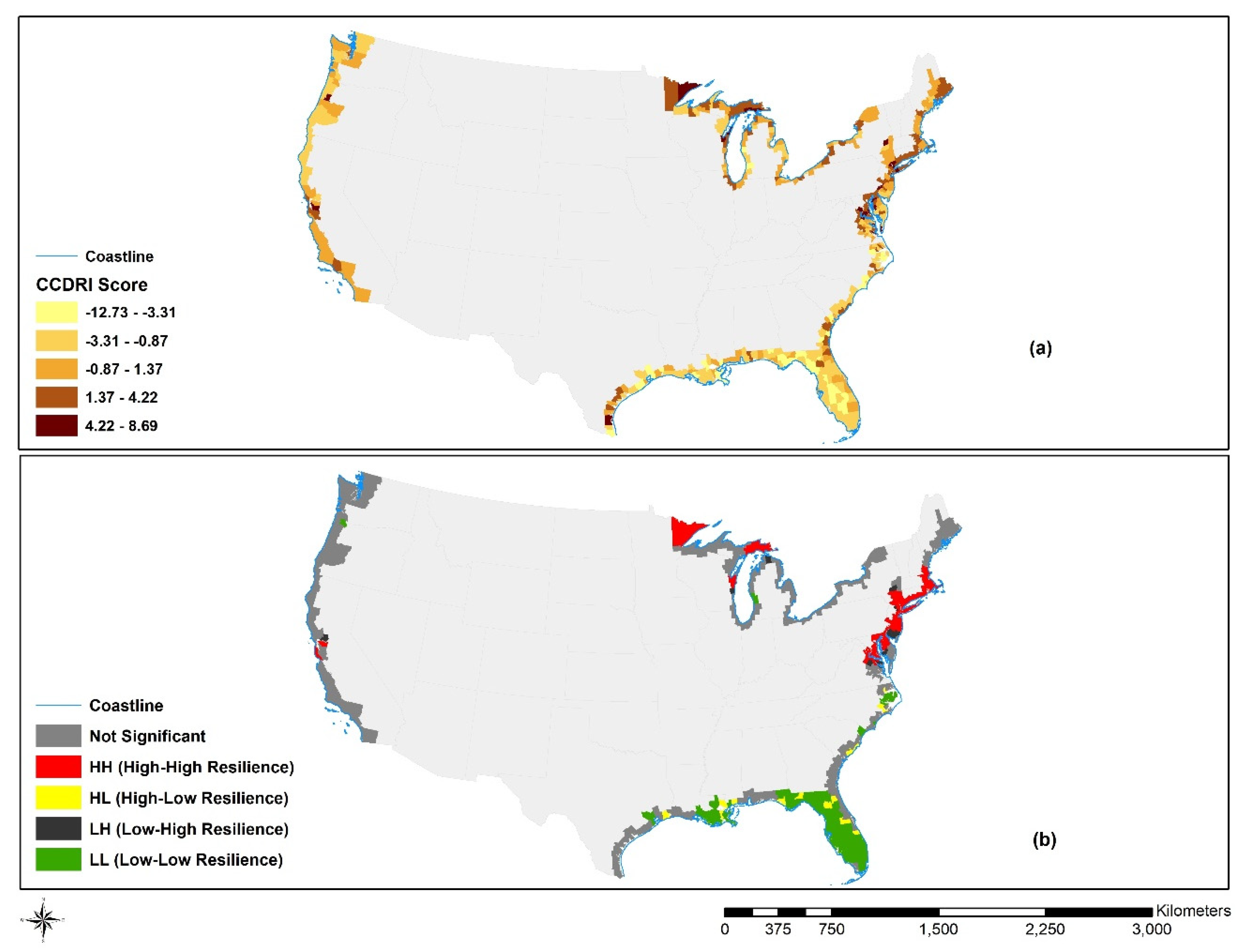
In this study, we assessed the community disaster resilience using the composite index (CCDRI) constructed from the eight different components of disaster resilience. We then examined the spatial distribution of CCDRI score across the coastal counties of the US. The average CCDRI score is 0.00 with an approximately normally distributed score. The standard deviation of the CCDRI score is 2.83 and a smaller median value than mean (−0.32) with a smaller positive skewness (0.16) suggests that the distribution of CCDRI score has a little positive skewness. The minimum value of the CCDRI score is −12.73 (the least resilient) and the maximum value is 8.69 (the most resilient).
The spatial distribution of CCDRI scores varies regionally (Figure 2a). Using the natural breaks (Jenks) classification category in ArcGIS, the higher values (> 1.37) of CCDRI score are concentrated around the northeastern region of the US (mainly in Maryland, Virginia, Pennsylvania, and extending north into southern New York, northeastern Massachusetts, and Rhode Island). Other counties with high values are in the states around the Great Lakes (mainly in northern Michigan, northeastern Wisconsin, and Minnesota). Additionally, the western part of the coastal counties in the study area, which is comprised of three states including California, Oregon, and Washington, includes a few counties with high CCDRI scores. However, most of the coastal counties in these three states have low-moderate values of CCDRI score (values between −3.31 and 1.37). The lowest values of the CCDRI score (<−0.87) are mainly located at the southeastern region of the study area covering five states including Florida, Mississippi, Alabama, Louisiana, and northern part of Texas. The southern part of the state of Texas shows concentration of high CCDRI scores. We have also used local Moran’s I statistic (LISA) to examine the statistically significant clusters of disaster resilience among the coastal counties (Figure 2b). Like the spatial distribution of the CCDRI scores, the clusters of hot spots which correspond to high resilience communities in a high resilience neighborhood is located at the northeastern region of the study area and around some parts of the Great Lakes (northern Michigan, northeastern Wisconsin, and Minnesota). However, there are some spatial outliers of low–high clusters (low resilience in a high resilience neighborhood) at the northeastern region as well. The cold spot clusters correspond to the low resilient counties in a low resilience neighborhood and are mostly located at the southeastern region of the country (Figure 2b). However, like the hot spots, there are some spatial outliers of high–low clusters that correspond to the high resilience in a low resilience neighborhood in this region as well.
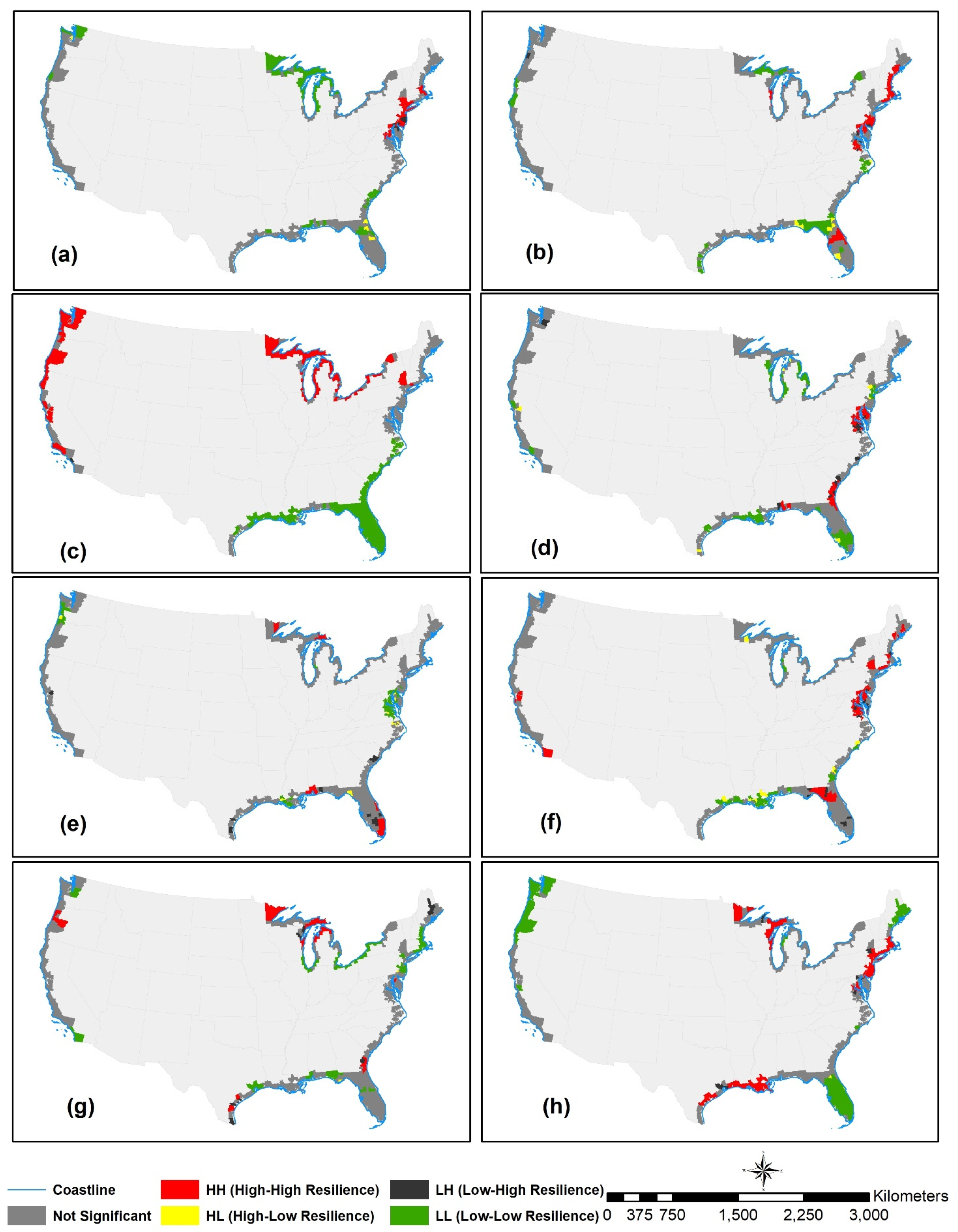
As discussed earlier, the CCDRI score is the combination of the eight resilience components that represent five dimensions of disaster resilience (Table 3). However, these components vary geographically depending on the local conditions. Figure 3 shows the hot spot and cold spot clusters of the eight resilience components. The spatial clusters of these components follow almost the same pattern of the spatial clusters of CCDRI scores as shown in (Figure 2b) with some exceptions. For example, the first component, the community capital-environmental-infrastructural dimension of disaster resilience that is comprised of local government revenues, percentage of urban area, and total length of major roads of a community, has hot spot clusters at the northeastern region (especially in and around New Jersey and New York) of the study area and cold spot clusters at the southeastern US and around the Great Lakes region (Figure 3a). Evidently, these northeastern coastal communities are mostly part of metropolitan areas with stronger community capitals and major road networks at their disposal than other communities in the study area. The social-infrastructural dimension (Component 2; Figure 3b), economic-community involvement dimension (Component 4; Figure 3d), and environmental-social dimension (Component 6; Figure 3f) have the almost similar pattern like Component 1, although a small cluster of hot spots at the southeastern region is shown (mainly in some parts of Florida and Georgia). Component 3 (social-environmental) shows hot spots around the Great Lakes and western part of the study area and cold spots at the southeastern region (Figure 3c). Component 7, that is mainly represented by the inverted hazard exposure and percent of voting age people participated in the last national election variable, shows statistically significant clusters of hotspots around the northern part of Great Lakes and cold spots around the northeastern as well as southeastern regions (Figure 3g) primarily suggesting that both northeastern and southeastern regions of the study area had high hazard exposure due to the repetitive disaster events such as hurricanes and flooding with high property damages compared to the northern part of the Great Lakes region. Affiliation with religious organizations that shows some form of community capital and is one of the primary variables of Component 8 has cold spot clusters mainly concentrated in Florida and western part of the study area (Figure 3h). The hot spot clusters of this component are mainly in the northeastern region and around Louisiana and Texas. Another dominant variable of Component 8 is the percent of wetlands in a community. The hot spots of Component 8 around the Louisiana–Texas region confirms the fact that this region has the highest amount of wetlands nationally.
3.2. Impacts of Community Disaster Resilience on Property Damages
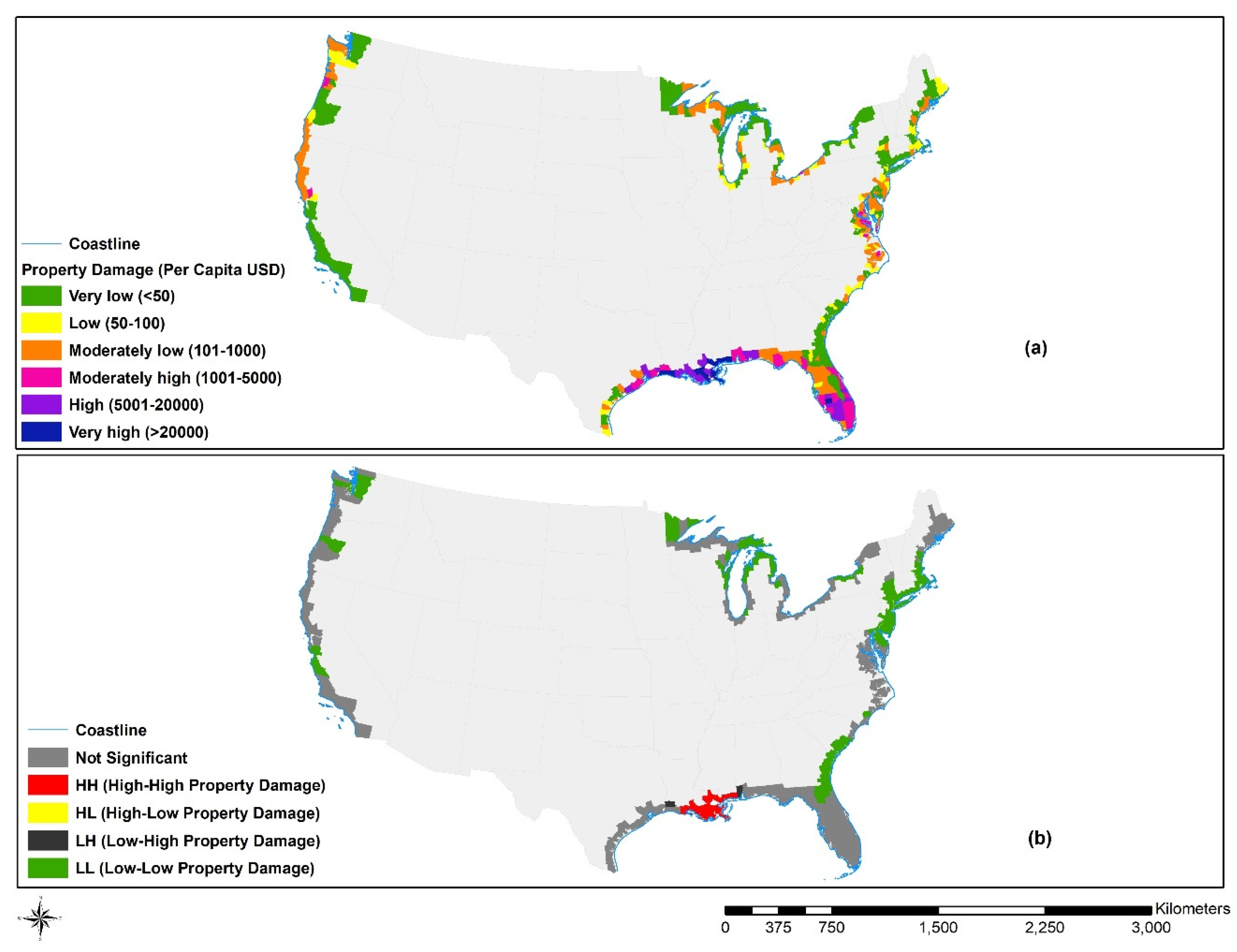
Since communities with higher resilience contribute to decrease disaster vulnerability and increase adaptive capacity as an effort to lessen the disaster impacts, it is our understanding that more resilient communities, as measured by the eight resilience components from the five different dimensions of disaster resilience, might have experienced less disaster impacts such as property damage and human life loss. As disaster casualties are considerably low in the US compared to other developing countries in the world, we tested this hypothesis with disaster property damage and by conducting the OLS and GWR regression analyses. In both OLS and GWR models, log transformed disaster property damage caused by five major coastal hazards between 2001 and 2010 was set as the dependent variable and eight resilience components were the explanatory/independent variables. Before doing the OLS and GWR, we examined the spatial distribution of property damage across the study area and the spatial clusters of damage using LISA in ArcGIS (Figure 4). We manually classified the property damage into six classes (from very low to very high) for the visualization purpose (Figure 4a). As shown in Figure 4a, high property damage values (>$5000) are concentrated around the southwestern Florida and Louisiana–Mississippi region. At the northeastern part of the study area, there are mainly low property damage counties caused by coastal disasters in the 10-year period (2001–2010) as seen around the Great Lakes and some parts of the western side of the study area. This pattern is further confirmed by the local Moran’s I statistic (LISA). Figure 4b shows that there is a statistically significant cluster of hot spots (high property damage in a high damage neighborhood) in the Louisiana–Mississippi region. The cold spots (low property damage in a low property damage neighborhood) are seen in the northeastern, some parts of the western side, and southeastern side (Georgia and Carolinas) of the study area.
We also analyzed the spatial pattern of the disaster property damage in the study area using the spatial autocorrelation (Moran’s I) tool in ArcGIS. A statistically significant (p < 0.001) Moran’s I score of 0.28 with a z-score of 15.095 suggests that property damage caused by coastal disasters is not equally distributed across the study area and the presence of the spatial autocorrelation problem in the property damage values. Therefore, a GWR model would better explain the relationship of the dependent and independent variables as GWR can model the spatial variations in the data by providing individual coefficients of each independent variables for all counties where OLS shows the overall influence of independent variables on the dependent variable. Furthermore, a GWR model can reveal the local characteristics of each community while minimizing the spatial autocorrelation problem. We employed a comparative analysis between the OLS and GWR model with the same set of dependent (per capita property damage) and independent variables (eight resilience components) to examine the impacts of resilience components on disaster property damage. Table 4 shows the average coefficient values and the standard deviation for all the communities of the GWR model and the coefficient values for the OLS model.
3.2.1. OLS Results
The impacts of resilience components on disaster property damage were initially examined using OLS. As shown in Table 4, statistically significant relationships are observed between the explanatory variables (eight resilience components) and the dependent variable (property damage). The OLS model explains 32% of the variance by regressing the eight resilience components against the disaster property damage. Six of the eight independent variables were found statistically significant in the OLS model with a negative direction. This negative relationship between the explanatory variables and the dependent variable suggests that there is an inverse relationship (less resilience corresponds to more property damage in a community) between them across the study area.
In the OLS model, the social-environmental component which is represented by the percentage of health insurance coverage and mean elevation of a community had the highest negative influence on the disaster property damage. A unit increase of the social-environmental resilience would decrease the disaster property damage by 42% (β = 0.42, p < 0.001) in the study area. This result supports our previous statement that higher elevation in the coastal areas maximizes disaster resiliency in a community. Additionally, residents covered by health insurance policy in a community tend to enhance community resilience. Environmental-community involvement (measured by the inverted hazard exposure and percent of voting age people participated in the last national election), community capital-environmental-infrastructural (measured by local government finances, urban area percentage, and total length of major roads in a community), and environmental-social (measured by inverted land lost percentage and a community’s effectiveness in communication) resilience components had strong negative impacts on the disaster property damage in the study area as shown in Table 4. A unit increase in each of these components would decrease the property damage caused by disasters about 25% each in the OLS model. In addition, more revenue generated by local government shows high resilience as they could aid local community during an emergency more effectively than others with resources available to them and therefore tend to experience less property damage. Similarly, environmental factors such as more urban areas and less land area lost in a community enhance overall resilience and hence correspond to less property damage as found in previous studies [47,51]. Additionally, this study also found that a unit increase in the housing-economic component of disaster resilience would decrease the property damage by 13% in the study area in the OLS model (Table 4). Infrastructural capacities of a community tend to minimize losses due to disasters and strengthen the overall resilience of the community as found in this study. Major roads, hospital beds, and vacant houses for rent as the dominant variables in the infrastructural dimension of resilience contribute to enhance the community disaster resilience as evidenced in this research. Variables such as housing units that are more recently built and that are not mobile homes (social-infrastructural, Component 2) also have a significant effect on decreasing property damage caused by disasters. Housing units that are comparatively new and strong tend to sustain the impacts of coastal hazards compared to the housing structures that are old as expected. People voted in a recent election correspond to a community that is more engaged which enhances overall community resilience and decreases disaster property damage in the study area as expected.
3.2.2. GWR Results
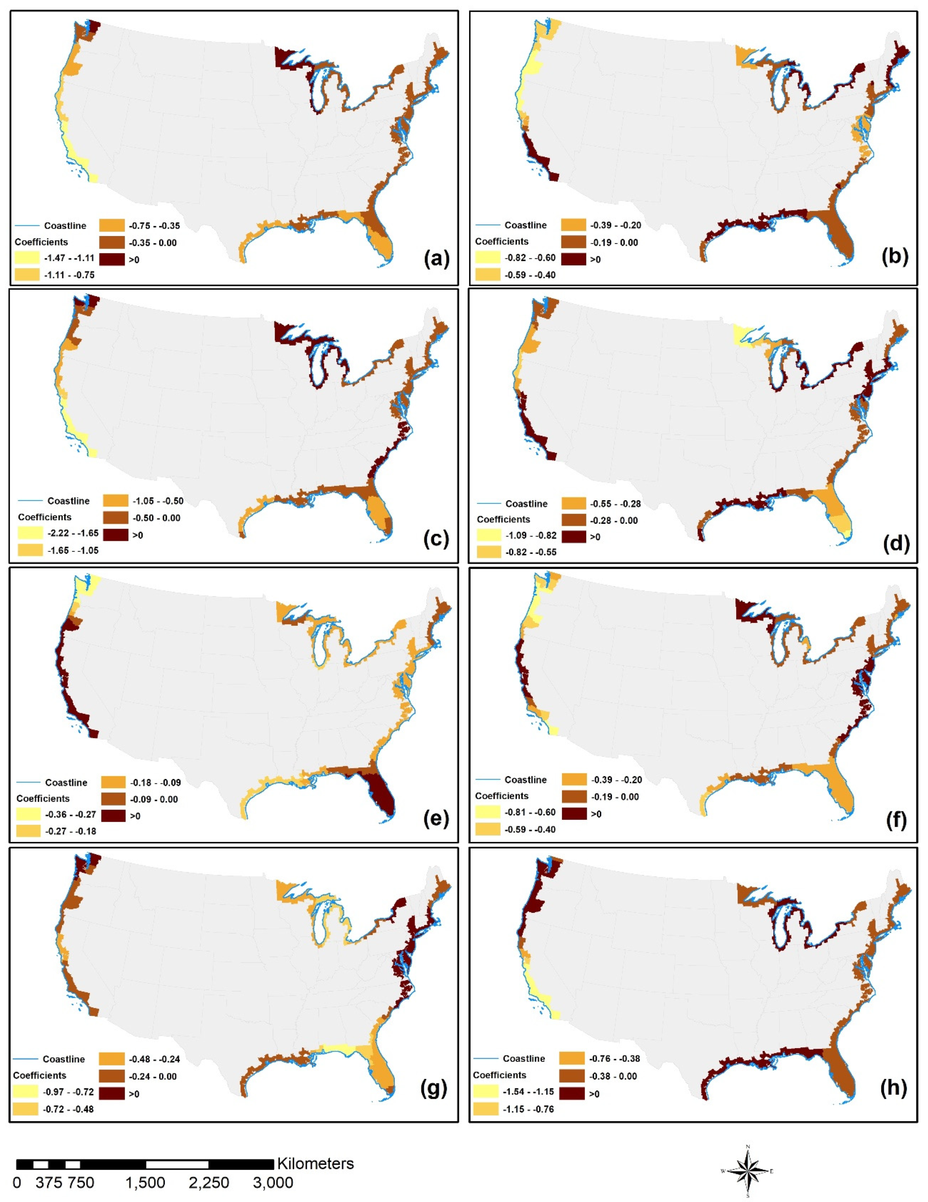
All the components that are strongly and negatively related with property damage in the OLS model also negatively impact the property damage in the GWR model as seen in Table 4. However, in the GWR model, considering local differences, demonstrates a massive improvement in explained variance from 32% in OLS model to 72%. All eight resilience components significantly influence the decrease of disaster property damage. The most influential variable in the GWR model is the community capital-environmental-infrastructural component (Table 4) as one-unit increase in this component would decrease the property damage by 29% on average across the study area followed by the Social-Environmental component. A one-unit increase in the social-environmental component would result in 19% decrease on average in the property damage in the coastal communities. The environmental-community involvement component, measured by the inverted hazard exposure and percent of voting age people voted in the last election in a community, are other influential variables in the GWR model as shown in Table 4. A unit increase in this component would decrease the property damage value by 14% in the GWR model on average in the study area. However, since the GWR model accounts for the geographical location and variations in the data, the influence of the independent variables varies across the study area. Additionally, a much higher R2 value in the GWR model suggests that there might be spatial non-stationarity between the property damage and the eight components of disaster resilience as shown in the previous study [53]. The local coefficients are mapped (Figure 5) to show the spatially varying relationships between the property damage and eight resilience components. Figure 5 shows the spatial distributions of the coefficients in the GWR model. As expected, most of the study area have negative values for all the coefficients of the dependent variable which suggests an overall negative relationship between the dependent and independent variables. The spatial pattern of the coefficients suggests that the relationships between the dependent and independent variables are not constant in the study area. Moreover, Figure 5 identifies areas with high negative individual coefficients for each component. For example, the southwestern part of the study area (in California) has higher negative coefficients of the community capital-environmental-infrastructural dimension compared to the northeastern part of the study area which suggests that the former area has a larger impact on property damage reduction than the latter for this dimension. However, this is just the opposite in case of the social-infrastructural dimension as evidenced in Figure 5b. Coefficients in the social-environmental component has larger negative values in the southwestern and southeastern part of the study area as this dimension is represented by the mean elevation and percentage of health insurance policyholders (Figure 5c). Coefficients in the housing-economic and environmental-community involvement components (Figure 5e,g, respectively) have almost similar patterns of coefficient distributions. The former has larger negative coefficients in the northern and southwestern parts of the study area where the latter has smaller negative coefficients in the southern part only. Both these components have negative coefficients around the Great Lakes area.
3.2.3. Comparison between OLS and GWR Models
The R2 and the AICc values of OLS and GWR are shown in the Table 4. The GWR model has higher R2 value (0.72) and lower AICc value (895.516) than the OLS (R2 value is 0.32, and AICc is 1060.035) suggesting better overall performance for the GWR model. The higher R2 value in the GWR model shows that the GWR models the relationship between disaster property damage and resilience components better than the OLS. The lower AICc value in the GWR model than the OLS model indicates a closer approximation of the GWR model to the real-life.
However, the R2 and AICc values only provide information about the overall performances of the models. To check the spatial non-stationarity in the study area, we also calculated the spatial autocorrelation (global Moran’s I) of the residuals of both OLS and GWR models. As shown in Table 4, there is a statistically significant global Moran’s I value of OLS’ residuals of 0.51. However, in the GWR model, the Moran’s I value significantly decreased to only 0.13. Therefore, the assumption of residual independence is violated in the OLS model.
We have also mapped the Local R2 values of the GWR model (Figure 6). As Figure 6 shows, the local R2 values vary spatially across the study area suggesting that the abilities of resilience components to explain disaster property damage is not constant and vary spatially. Additionally, the local R2 values are greater at more than 80% areas than the global (OLS) R2 value of 0.32. These results confirm that disaster resilience is inversely related with disaster property damage as found in the study area and this relationship changes across the space.
4. Discussion
The CCDRI acts as a reference-point for inspecting the present standing of disaster resilience of the coastal communities in the conterminous US. Even though there is no definitive threshold CCDRI score for a community to be resilient, communities could compare their respective CCDRI scores with neighboring communities. Northeastern communities pose higher disaster resilience compared to the southeastern where western part of the coast demonstrates moderate level of resilience measured by CCDRI. To answer our first research question, there is, in fact, a spatial/geographical pattern of community disaster resilience in the coastal US as shown by the CCDRI. As the results shown above, the different disaster resilience components follow almost the similar pattern. Additionally, the spatial patterns of the multidimensional resilience as demonstrated in this study could have a great impact on local policies. Local governments as well as policymakers could focus on specific areas where they can improve to enhance overall community resilience. For example, coastal counties in Virginia, Maryland, and New Jersey (at the northeastern part of the study area) show weaker housing-economic resilience. Policies targeting increasing the number of hospital beds, temporary shelters for emergency situation, and minimizing the wage gap between male and female earners (as these variables primarily represent the housing-economic dimension) could enhance their resilience in this dimension as well as their composite disaster resilience. On the other hand, the southeastern Florida is stronger in this dimension (Figure 3e), so this region could focus on improving the health insurance coverage percentage (as part of Component 3) in their communities by taking necessary steps to ensure more health insurance coverage in the community (e.g., government subsidy on health insurance policies) as a measure to enhance overall disaster resilience in this region. Furthermore, the resilience variables used in this research could be easily assessed in future to measure the changes in disaster resilience in coastal communities as well as to compare the overall resilience over time.
However, it should be noted that not all the variables that represent community resilience are applicable for a large geographic area [10] like this study. Some variables might not be important at the local context even though they have previously been used to measure disaster resilience at the national scale. For example, as demonstrated by Cutter and her team [23], speaking proficiency in English might not be applicable in southeast Florida as a resilience variable since information is available both in English and Spanish in this region.
This study also explores the relationships between the resilience indicators and disaster loss in the study area. In doing this, this study employs both global regression model (OLS) and local regression model (GWR) to portray the overall influence of the resilience indicators (as measured by the eight resilience components) on disaster property damage, and their spatially varying relationships, respectively. As expected, statistically significant negative relationships were found between the resilience indicators and property damage in both models suggesting more resilient communities sustain less property damages from disasters in the study area. However, the influences of different resilience indicators on reducing the property damage were different in GWR model than in OLS model. This is due to the fact that unlike GWR, OLS does not consider the spatial variations in the resilience indicators and disaster property damages. Community resilience to disasters varies from place to place and as a natural process, natural disasters and property damages caused by these disasters demonstrate high spatial heterogeneity as well. Therefore, it is difficult to illustrate the relationships between disaster resilience and property damage with conventional regression methods like OLS which provides an estimated mean value for the overall study area irrespective of spatial patterns. Nevertheless, the varying heterogeneous influences of resilience indicators on disaster property damage have rarely been studied previously. The results found in this study suggest significant spatially varying relationship between resilience indicators and disaster property damage in the study area. GWR is found to be an effective method to ascertain spatial non-stationarity when it comes to examine the influence of resilience indicators on property damage caused by disasters. With higher overall R2 value and better model-fit (lower AICc value) than the OLS, GWR model provides fresh insights into the dynamic relationships between community resilience and impacts from disaster in this study. More importantly, the results of the GWR model (Section 3.2.2) could also benefit the emergency managers and local leaders in the context of disaster plan preparedness and policies. Emergency managers could identify the specific areas in need of improvement to enhance the overall disaster resilience of the local community. Evidently, disaster management policies need to be customized to the individual communities to reduce disaster impacts and increase community resilience to disasters. As the GWR models the local relationships between the dependent and independent variables, policies based on the GWR results would be more effective as it would reflect the local circumstances than an overall national policy. Accordingly, GWR provides policymakers and managers with a set of specific coefficients to make decisions in their communities. Therefore, the spatial relationship between the disaster resilience indicators and impacts from disasters (such as property damage) should be considered to enhance overall community resilience and reduce disaster losses subsequently.
5. Conclusions
In this study, we first measured the overall disaster resilience of the coastal communities in the US based on the variables that has been used in previous studies and represent five different dimensions of disaster resilience (social, economic, community capital and engagement, housing/infrastructural, and environmental) by creating composite index scores of community resilience using PCA. The PCA provides eight inter-dimensional components. The results of the study suggest that community resilience to coastal disasters vary across the study area where northeastern coastal communities are comparatively more resilient to disasters than southeastern communities.
Additionally, this research reveals the importance of considering spatial variations of disaster resilience which has been overlooked in previous studies when it comes to community resilience to disasters in the US. Firstly, the spatial pattern analysis of the local communities (LISA) provides evidences that northern communities in the study area are in a high resilience cluster zone and southern communities are within a low resilience cluster zone. This pattern was almost similar in the case of eight inter-dimensional resilience components used in this study. The results provide practical insights to specify resources that can make coastal communities more resilient to coastal hazards. Differences in different resilience dimensions correspond to levels of disaster resilience (from low to high). Therefore, attentions need to be directed towards less resilient communities with specific considerations and guidelines to augment overall disaster resilience as well as curtail disaster impacts.
Previous studies used different variables to represent different resilience dimensions and to measure overall disaster resilience of communities. However, little to no justification has been provided in using those proxy variables of resilience. In this study, we overcame this knowledge gap by examining the influence of inter-dimensional resilience components on actual disaster impacts (property damage caused by disasters) in the study area. Generally, the higher the disaster resilience, the lower the adverse impacts of disasters sustained by the communities. We tested this hypothesis by regressing the eight resilience components against the disaster property damage in the study area which also provides as a means of justification for using these components for measuring composite disaster resilience of the study area. Moreover, we used both global (OLS) and local (GWR) models to test this hypothesis as global models are not capable of capturing the spatial variation in the data. Results from both models suggest that resilience components used in this study have statistically significant impacts on reducing the disaster property damage in the study area. However, GWR model performed better in explaining the variance of the dependent variable and proved to be the better fit of the data than the OLS model. By considering the spatial variations in inter-dimensional resilience components, GWR model shows that eight components of disaster resilience have varying impacts in local communities.
The results in this study provide an important revelation that spatial variations of resilience components should be considered in the field of disaster resilience especially in a larger geographic area where dimensions of resilience differ greatly. Furthermore, each community in the study area has a discrete characteristics of disaster resilience. Therefore, communities need to prioritize their strategies and policies to increase overall disaster resilience. For example, communities that are more vulnerable on the housing and infrastructural dimension should prioritize on increasing their infrastructural capacities such as constructing and ensuring proper maintenance of major roads, increasing the capacities of the local hospitals, etc. over other dimensions to reduce vulnerability and disaster impacts. Overall, this study could provide local emergency managers and decision-makers with unique directions toward a more proactive policy approach at the local level for enhancing community disaster resilience and subsequently minimizing adverse impacts of disasters. Finally, some other physical factors such as average annual rainfall could be added in future studies as a proxy variable to measure community resilience to disasters and the disaster impacts on the coastal communities which might produce better results.
Author Contributions
Conceptualization, Weibo Liu and Shaikh Abdullah Al Rifat; methodology, Shaikh Abdullah Al Rifat and Weibo Liu; formal analysis, Shaikh Abdullah Al Rifat and Weibo Liu; writing—original draft, Shaikh Abdullah Al Rifat and Weibo Liu; writing—review and editing, Weibo Liu. All authors have read and agreed to the published version of the manuscript.
Funding
This research received no external funding.
Acknowledgments
We would like to thank the anonymous reviewers and editors for providing valuable comments and suggestions which helped improve the manuscript greatly.
Conflicts of Interest
The authors declare no conflict of interest.
References
- Auld, H. Disaster risk reduction under current and changing climate conditions. Bull. World Meteorol. Organ. 2008, 57, 118–125. [Google Scholar]
- Costanza, R.; Farley, J. Ecological economics of coastal disasters: Introduction to the special issue. Ecol. Econ. 2007, 63, 249–253. [Google Scholar] [CrossRef]
- Intergovernmental Panel on Climate Change (IPCC). Managing the Risks of Extreme Events and Disasters to Advance Climate Change Adaptation; Cambridge University Press: Cambridge, UK; New York, NY, USA, 2012. [Google Scholar] [CrossRef]
- Lam, N.S.N.; Arenas, H.; Brito, P.L.; Liu, K. Assessment of vulnerability and adaptive capacity to coastal hazards in the Caribbean Region. J. Coast. Res. 2014, 70, 473–478. [Google Scholar] [CrossRef]
- Lloyd, M.G.; Peel, D.; Duck, R.W. Towards a social-ecological resilience framework for coastal planning. Land Use Policy 2013, 30, 925–933. [Google Scholar] [CrossRef]
- Knutson, T.R.; McBride, J.L.; Chan, J.; Emanuel, K.; Holland, G.; Landsea, C.; Held, I.; Kossin, J.P.; Srivastava, A.K.; Sugi, M. Tropical cyclones and climate change. Nat. Geosci. 2010, 3, 157–163. [Google Scholar] [CrossRef] [Green Version]
- Nicholls, R.J.; Cazenave, A. Sea-level rise and its impact on coastal zones. Science 2010, 328, 1517–1520. [Google Scholar] [CrossRef]
- Rifat, S.A.A.; Liu, W. Quantifying Spatiotemporal Patterns and Major Explanatory Factors of Urban Expansion in Miami Metropolitan Area During 1992–2016. Remote Sens. 2019, 11, 2493. [Google Scholar] [CrossRef] [Green Version]
- Adger, W.N. Social and ecological resilience: Are they related? Prog. Hum. Geogr. 2000, 24, 347–364. [Google Scholar] [CrossRef]
- Cutter, S.L.; Burton, C.G.; Emrich, C.T. Disaster Resilience Indicators for Benchmarking Baseline Conditions. J. Homel. Secur. Emerg. Manag. 2010, 7, 1–22. [Google Scholar] [CrossRef]
- Lam, N.S.N.; Pace, K.; Campanella, R.; LeSage, J.; Arenas, H. Business return in New Orleans: Decision making amid post-Katrina uncertainty. PLoS ONE 2009, 4, e6765. [Google Scholar] [CrossRef] [Green Version]
- Lam, N.S.N.; Qiang, Y.; Arenas, H.; Brito, P.; Liu, K.B. Mapping and assessing coastal resilience in the Caribbean region. Cartogr. Geogr. Inf. Sci. 2015, 42, 315–322. [Google Scholar] [CrossRef]
- National Research Council. Disaster Resilience: A National Imperative; The National Academies Press: Washington, DC, USA, 2012. [Google Scholar]
- Adger, W.N.; Hughes, T.P.; Folke, C.; Carpenter, S.R.; Rockström, J. Social-ecological resilience to coastal disasters. Science 2005, 309, 1036–1039. [Google Scholar] [CrossRef] [PubMed] [Green Version]
- Aldrich, D.P. Building Resilience: Social Capital in Post-Disaster Recovery; University of Chicago Press: Chicago, IL, USA, 2012. [Google Scholar]
- Bruneau, M.; Chang, S.E.; Eguchi, R.T.; Lee, G.C.; O’Rourke, T.D.; Reinhorn, A.M.; Shinozuka, M.; Tierney, K.; Wallace, W.A.; Von Winterfeldt, D. A Framework to Quantitatively Assess and Enhance the Seismic Resilience of Communities. Earthq. Spectra 2003, 19, 733–752. [Google Scholar] [CrossRef] [Green Version]
- Manyena, S.B. The concept of resilience revisited. Disasters 2006, 30, 434–450. [Google Scholar] [CrossRef] [PubMed]
- Norris, F.H.; Stevens, S.P.; Pfefferbaum, B.; Wyche, K.F.; Pfefferbaum, R.L. Community resilience as a metaphor, theory, set of capacities, and strategy for disaster readiness. Am. J. Community Psychol. 2008, 41, 127–150. [Google Scholar] [CrossRef] [PubMed]
- Sherrieb, K.; Norris, F.H.; Galea, S. Measuring Capacities for Community Resilience. Soc. Indic. Res. 2010, 99, 227–247. [Google Scholar] [CrossRef]
- Sherrieb, K.; Louis, C.A.; Pfefferbaum, R.L.; Pfefferbaum, B.J.D.; Diab, E.; Norris, F.H. Assessing community resilience on the US coast using school principals as key informants. Int. J. Disaster Risk Reduct. 2012, 2, 6–15. [Google Scholar] [CrossRef]
- Tierney, K. Disaster Governance: Social, Political, and Economic Dimensions. Annu. Rev. Environ. Resour. 2012, 37, 341–363. [Google Scholar] [CrossRef]
- Cutter, S.L.; Barnes, L.; Berry, M.; Burton, C.; Evans, E.; Tate, E.; Webb, J. A place-based model for understanding community resilience to natural disasters. Glob. Environ. Chang. 2008, 18, 598–606. [Google Scholar] [CrossRef]
- Cutter, S.L.; Ash, K.D.; Emrich, C.T. The geographies of community disaster resilience. Glob. Environ. Chang. 2014, 29, 65–77. [Google Scholar] [CrossRef]
- Folke, C. Resilience: The emergence of a perspective for social-ecological systems analyses. Glob. Environ. Chang. 2006, 16, 253–267. [Google Scholar] [CrossRef]
- Ross, A.D. Local Disaster Resilience: Administrative and Political Perspectives; Routledge: New York, NY, USA, 2013. [Google Scholar]
- Engle, N.L. Adaptive capacity and its assessment. Glob. Environ. Chang. 2011, 21, 647–656. [Google Scholar] [CrossRef]
- Turner, B.L.; Kasperson, R.E.; Matsone, P.A.; McCarthy, J.J.; Corell, R.W.; Christensen, L.; Eckley, N.; Kasperson, J.X.; Luers, A.; Martello, M.L.; et al. A framework for vulnerability analysis in sustainability science. Proc. Natl. Acad. Sci. USA 2003, 100, 8074–8079. [Google Scholar] [CrossRef] [PubMed] [Green Version]
- McCarthy, J.J.; Canziani, O.F.; Leary, N.A.; Dokken, D.J.; White, K.S. Climate Change 2001: Impacts, Adaptation, and Vulnerability: Contribution of Working Group II to the Third Assessment Report of the Intergovernmental Panel on Climate Change; Cambridge University Press: Cambridge, UK, 2001; Volume 2. [Google Scholar]
- Klein, R.J.T.; Nicholls, R.J.; Thomalla, F. Resilience to natural hazards: How useful is this concept? Environ. Hazards 2003, 5, 35–45. [Google Scholar] [CrossRef]
- Cutter, S.L.; Boruff, B.J.; Shirley, W.L. Social vulnerability to environmental hazards. Soc. Sci. Q. 2003, 84, 242–261. [Google Scholar] [CrossRef]
- Cutter, S.L.; Barnes, L.; Berry, M.; Burton, C.; Evans, E.; Tate, E.; Webb, J. Community and Regional Resilience: Perspectives from Hazards, Disasters, and Emergency Management. Geography 2008, 1, 2301–2306. [Google Scholar] [CrossRef] [Green Version]
- Hossain, M.K.; Meng, Q. A thematic mapping method to assess and analyze potential urban hazards and risks caused by flooding. Comput. Environ. Urban Syst. 2020, 79, 101417. [Google Scholar] [CrossRef]
- Sempier, T.; Swann, L.; Emmer, R.; Sempier, S.H.; Schneider, M. A Community Self-Assessment; MASGP-08-014, Mississippi-Alabama, Sea Grant Consortium. 2010; Available online: http://www.southernclimate.org/documents/resources/Coastal_Resilience_Index_Sea_Grant.pdf (accessed on 22 June 2020).
- Burton, C.G. A Validation of Metrics for Community Resilience to Natural Hazards and Disasters Using the Recovery from Hurricane Katrina as a Case Study. Ann. Assoc. Am. Geogr. 2015, 105, 67–86. [Google Scholar] [CrossRef]
- Tate, E. Social vulnerability indices: A comparative assessment using uncertainty and sensitivity analysis. Nat. Hazards 2012, 63, 325–347. [Google Scholar] [CrossRef]
- Archer, J.H.; Knecht, R.W. The US national coastal zone management program—Problems and opportunities in the next phase. Coast. Manag. 1987, 15, 103–120. [Google Scholar] [CrossRef]
- Cutter, S.L.; Derakhshan, S. Temporal and spatial change in disaster resilience in US counties, 2010–2015*. Environ. Hazards 2018, 19, 10–29. [Google Scholar] [CrossRef]
- Kulig, J.C.; Edge, D.S.; Ivan, T.; Lightfoot, N.; Reimer, W. Community Resiliency: Emerging Theoretical Insights. J. Community Psychol. 2013, 41, 758–775. [Google Scholar] [CrossRef]
- Peacock, W.G. Final Report: Advancing the Resilience of Coastal Localities; Texas A&M University Press: College Station, TX, USA, 2010. [Google Scholar]
- Yoon, D.K.; Kang, J.E.; Brody, S.D. A measurement of community disaster resilience in Korea. J. Environ. Plan. Manag. 2016, 59, 436–460. [Google Scholar] [CrossRef]
- Burger, J.; Gochfeld, M.; Jeitner, C.; Pittfield, T.; Donio, M. Trusted information sources used during and after superstorm sandy: TV and radio were used more often than social media. J. Toxicol. Environ. Health Part A 2013, 76, 1138–1150. [Google Scholar] [CrossRef] [Green Version]
- Colten, C.E.; Kates, R.W.; Laska, S.B. Community Resilience: Lessons from New Orleans and Hurricane Katrina. CARRI Rep. 2008, 3, 2–4. Available online: https://rwkates.org/pdfs/a2008.03.pdf (accessed on 23 June 2020).
- Chandra, A.; Acosta, J.; Howard, S.; Uscher-Pines, L.; Williams, M.; Yeung, D.; Garnett, J.; Meredith, L.S. Building community resilience to disasters: A way forward to enhance national health security. Rand Health Q. 2011, 1. [Google Scholar] [CrossRef]
- Lam, N.S.N.; Reams, M.; Li, K.; Li, C.; Mata, L.P. Measuring Community Resilience to Coastal Hazards along the Northern Gulf of Mexico. Nat. Hazards Rev. 2016, 17, 04015013. [Google Scholar] [CrossRef] [Green Version]
- Morrow, B.H. Community Resilience: A Social Justice Perspective; CARRI Research Report; CARRI: Oak Ridge, TN, USA, 2008. [Google Scholar]
- Birkmann, J.; Cardona, O.D.; Carreño, M.L.; Barbat, A.H.; Pelling, M.; Schneiderbauer, S.; Kienberger, S.; Keiler, M.; Alexander, D.; Zeil, P.; et al. Framing vulnerability, risk and societal responses: The MOVE framework. Nat. Hazards 2013, 67, 193–211. [Google Scholar] [CrossRef]
- Cai, H.; Lam, N.S.N.; Zou, L.; Qiang, Y.; Li, K. Assessing community resilience to coastal hazards in the Lower Mississippi River Basin. Water 2016, 8, 46. [Google Scholar] [CrossRef] [Green Version]
- Hossain, M.K.; Meng, Q. A fine-scale spatial analytics of the assessment and mapping of buildings and population at different risk levels of urban flood. Land Use Policy 2020, 99, 104829. [Google Scholar] [CrossRef]
- Nakagawa, Y.; Shaw, R. Social Capital: A Missing Link to Disaster Recovery Yuko. Int. J. Mass Emerg. Disasters 2004, 22, 5–34. [Google Scholar] [CrossRef]
- Baker, A. Creating an Empirically Derived Community Resilience Index of the Gulf of Mexico Region. Master’s Thesis, Louisiana State University, Baton Rouge, LA, USA, 2009. [Google Scholar]
- Cutter, S.L.; Ash, K.D.; Emrich, C.T. Urban–Rural Differences in Disaster Resilience. Ann. Am. Assoc. Geogr. 2016, 106, 1236–1252. [Google Scholar] [CrossRef]
- Doctor, D.H.; Doctor, K.Z. Spatial analysis of geologic and hydrologic features relating to sinkhole occurrence in Jefferson County, West Virginia. Carbonates Evaporites 2012, 27, 143–152. [Google Scholar] [CrossRef]
- Zhao, C.; Jensen, J.; Weng, Q.; Weaver, R. A geographically weighted regression analysis of the underlying factors related to the surface Urban Heat Island Phenomenon. Remote Sens. 2018, 10, 1428. [Google Scholar] [CrossRef] [Green Version]
Figure 1.
Map of the study area.

Figure 2.
The spatial distribution of (a) composite community disaster resilience index (CCDRI) scores and (b) clusters of hot and cold spots of CCDRI scores.
Figure 2.
The spatial distribution of (a) composite community disaster resilience index (CCDRI) scores and (b) clusters of hot and cold spots of CCDRI scores.

Figure 3.
Clusters of hot and cold spots of eight community resilience components: (a) community capital-environmental-infrastructural; (b) social-infrastructural; (c) social-environmental; (d) economic-community involvement; (e) housing-economic; (f) environmental-social; (g) environmental-community involvement; (h) community capital-environmental.

Figure 4.
The spatial distribution of (a) property damage values and (b) clusters of hot and cold spots of property damage in the study area.
Figure 4.
The spatial distribution of (a) property damage values and (b) clusters of hot and cold spots of property damage in the study area.

Figure 5.
The spatial distribution of coefficients of the eight community resilience components in the GWR model: (a) community capital-environmental-infrastructural; (b) social-infrastructural; (c) social-environmental; (d) economic-community involvement; (e) housing-economic; (f) environmental-social; (g) environmental-community involvement; and (h) community capital-environmental.

Figure 6.
The spatial distribution of local R2 values in the GWR model.


Table 1.
Data sources and time periods used for indicators of disaster resilience index.
| Number | Dataset | Time Period | Data Provider |
|---|---|---|---|
| 1 | County and City Data Book | 2007 | US Census Bureau |
| 2 | Decennial Census | 2000, 2010 | |
| 3 | Tiger/Line | 2010 | |
| 4 | American Community Survey Five-Year Estimates | 2006–2010 | |
| 5 | USA Counties Database | 2007 | |
| 6 | Global Multi-resolution Terrain Elevation Data | 2010 | US Geological Survey |
| 7 | National Land Cover Dataset | 2001, 2011 | |
| 8 | Exposure and Damage Database | 2001–2010 | The US National Centers for Environmental Information (NCEI) |
| 9 | Religious Congregations and Membership Study | 2010 | Association of Religion Data Archives |
Table 2.
Resilience variables with description and justification. Dataset numbers correspond to the numbers in Table 1.
Table 2.
Resilience variables with description and justification. Dataset numbers correspond to the numbers in Table 1.
| Variable Description | Resilience Dimension | Justification | Dataset |
|---|---|---|---|
| Percent of females (inverted) | Social resilience | (Cutter, Boruff, and Shirley 2003; Yoon, Kang, and Brody 2016) [30,40] | 2 |
| Percent of population below 65 years old with health insurance | (Cutter, Ash, and Emrich 2014) [23] | 5 | |
| Percent of households with telephone service | (Burger et al. 2013; Colten, Kates, and Laska 2008) [41,42] | 4 | |
| Percent of households with at least one vehicle | (Peacock 2010) [39] | 4 | |
| Physicians per 10,000 persons | (Chandra et al. 2011) [43] | 4 | |
| Gini coefficient (inverted) | Economic resilience | (Cutter, Ash, and Emrich 2014) [23] | 4 |
| Percent of labor force employed by federal government | (Cutter, Ash, and Emrich 2014) [23] | 4 | |
| Absolute difference between male and female median income (inverted) | (Sherrieb, Norris, and Galea 2010) [19] | 2 | |
| Percent of employees not in farming, fisheries, forestry, extractive industry, or tourism | (Sherrieb, Norris, and Galea 2010) [19] | 4 | |
| Percent of workforce that is employed | (Lam et al. 2016) [44] | 4 | |
| Percent of population not foreign-born that came to the US after 2005 | Community engagement and capital resilience | (Norris et al. 2008) [18] | 4 |
| Local government finances, revenue per capita | (Lam et al. 2016) [44] | 1 | |
| Percent of population born in the same state of current residence | (Norris et al. 2008) [18] | 4 | |
| Percent of population affiliated with a religious organization | (Morrow 2008) [45] | 9 | |
| Percent of voting age population voted in 2008 election | (Morrow 2008; Peacock 2010) [39,45] | 5 | |
| Percent of housing units not mobile home | Housing/infrastructural resilience | (Cutter, Boruff, and Shirley 2003; Lam et al. 2016) [30,44] | 4 |
| Percent of vacant housing units for rent | (Cutter, Burton, and Emrich 2010) [10] | 4 | |
| Hospital beds per 10,000 persons | (Birkmann et al. 2013) [46] | 1, 2 | |
| Total length of roads per sq. km. | (Lam et al. 2016) [44] | 3 | |
| Percent of housing units built after 2000 | (Cutter, Burton, and Emrich 2010) [10] | 4 | |
| Percent of land in wetlands | Environmental resilience | (Cutter, Ash, and Emrich 2014) [23] | 7 |
| Percent of land lost between 2001-2011 (inverted) | (Lam et al. 2016) [44] | 7 | |
| Mean elevation of the county (meter) | (Cai et al. 2016; Hossain and Meng 2020) [47,48] | 6 | |
| Hazard exposure (inverted) | (Lam et al. 2016; Cai et al. 2016) [44,47] | 8 | |
| Percent of urban area | (Cai et al. 2016) [47] | 7 |
Table 3.
Identified components and dominant variables from principal component analysis (PCA).
| Component Number | Component Name | % Variation Explained | Dominant Variables |
|---|---|---|---|
| 1 | Community Capital-Environmental-Infrastructural | 18.32 | Local government finances, revenue per capita; percent of urban area; total length of roads per sq. km. |
| 2 | Social-Infrastructural | 13.15 | Physicians per 10,000 persons; percent of housing units not mobile home; percent of housing units built after 2000 |
| 3 | Social-Environmental | 11.26 | Percent of population below 65 years old with health insurance; mean elevation of the county (meter) |
| 4 | Economic-Community Involvement | 7.72 | Percent of labor force employed by federal government; percent of population not foreign-born that came to the US after 2005 |
| 5 | Housing-Economic | 5.57 | Hospital beds per 10,000 persons; percent of vacant housing units for rent; absolute difference between male and female median income (inverted) |
| 6 | Environmental-Social | 4.91 | Percent of land lost between 2001–2011 (inverted); percent of households with telephone service |
| 7 | Environmental-Community Involvement | 4.76 | Hazard exposure (inverted); percent of voting age population voted in 2008 election |
| 8 | Community Capital-Environmental | 4.1 | Percent of population affiliated with a religious organization; percent of land in wetlands |
Table 4.
Impacts of disaster resilience components on property damages caused by coastal hazards using ordinary least squares (OLS) and geographically weighted regression (GWR) models.
Table 4.
Impacts of disaster resilience components on property damages caused by coastal hazards using ordinary least squares (OLS) and geographically weighted regression (GWR) models.
| Coefficient (OLS) (β) | Coefficient (GWR) | ||
|---|---|---|---|
| Average (Mean β) | Standard Deviation | ||
| Constant | 2.07 *** | 1.95 | 0.62 |
| Community Capital-Environmental-Infrastructural | −0.24 *** | −0.29 | 0.27 |
| Social-Infrastructural | −0.09 * | −0.09 | 0.23 |
| Social-Environmental | −0.42 *** | −0.19 | 0.53 |
| Economic-Community Involvement | −0.07 | −0.09 | 0.32 |
| Housing-Economic | −0.13 ** | −0.08 | 0.18 |
| Environmental-Social | −0.24 *** | −0.1 | 0.26 |
| Environmental-Community Involvement | −0.25 *** | −0.14 | 0.35 |
| Community Capital-Environmental | 0.07 | −0.01 | 0.3 |
| R-square | 0.32 | 0.72 | |
| Adjusted R-square | 0.31 | 0.63 | |
| AICc | 1060.035 | 895.516 | |
| Global Moran’s I of Residuals | 0.51 *** | 0.13 *** | |
Note: *** p < 0.001 level, ** p < 0.01 level, * p < 0.1 level.
© 2020 by the authors. Licensee MDPI, Basel, Switzerland. This article is an open access article distributed under the terms and conditions of the Creative Commons Attribution (CC BY) license (http://creativecommons.org/licenses/by/4.0/).
Share and Cite
MDPI and ACS Style
Rifat, S.A.A.; Liu, W. Measuring Community Disaster Resilience in the Conterminous Coastal United States. ISPRS Int. J. Geo-Inf. 2020, 9, 469. https://doi.org/10.3390/ijgi9080469
AMA Style
Rifat SAA, Liu W. Measuring Community Disaster Resilience in the Conterminous Coastal United States. ISPRS International Journal of Geo-Information. 2020; 9(8):469. https://doi.org/10.3390/ijgi9080469
Chicago/Turabian StyleRifat, Shaikh Abdullah Al, and Weibo Liu. 2020. "Measuring Community Disaster Resilience in the Conterminous Coastal United States" ISPRS International Journal of Geo-Information 9, no. 8: 469. https://doi.org/10.3390/ijgi9080469
Note that from the first issue of 2016, this journal uses article numbers instead of page numbers. See further details here.