
Abstract
Recently, an increasing body of work investigates networks with multiple types of links. Variants of such systems have been examined decades ago in disciplines such as sociology and engineering, but only recently have they been unified within the framework of multilayer networks. In parallel, many aspects of real systems are increasingly and routinely sensed, measured and described, resulting in many private, but also open data sets. In many domains publicly available repositories of open data sets constitute a great opportunity for domain experts to contextualise their privately generated data compared to publicly available data in their domain. We propose in this paper a methodology for multilayer network analysis in order to provide domain experts with measures and methods to understand, evaluate and complete their private data by comparing and/or combining them with open data when both are modelled as multilayer networks. We illustrate our methodology through a biological application where interactions between molecules are extracted from open databases and modelled by a multilayer network and where private data are collected experimentally. This methodology helps biologists to compare their private networks with the open data, to assess the connectivity between the molecules across layers and to compute the distribution of the identified molecules in the open network. In addition, the shortest paths which are biologically meaningful are also analysed and classified.
Introduction
Network theory is an important tool for describing and analysing complex systems which are represented as mathematical graphs. It has many applications in social, biological, physical, information and engineering sciences (Fortunato 2010; Newman 2003; Gosak et al. 2017; Seminar 2019; Pavlopoulos et al. 2011; Djemili et al. 2017). For example, it has been used to capture interesting properties of many real networks, e.g. having a heavy-tailed degree distribution, having the small-world property, the existence of nodes playing central roles and/or the existence of modular structures (Newman 2003).
Recently, an increasing body of work investigates networks with multiple types of links, as well as the so-called “networks of networks”. Variants of such systems have been examined decades ago in disciplines such as sociology and engineering, but only recently have they been unified, along with other nomenclature, within the framework of multilayer networks defined by Kivelä et al. (2014).
In parallel many aspects of real systems are increasingly and routinely sensed, measured and described, resulting in many private, but also open data sets. By private data we mean data collected internally in a company or institution. Open data refers to the idea that some data should be freely available to everyone to use and republish at will, without restrictions from copyright, patents or other mechanisms of control.
In many domains publicly available repositories of open data sets constitute a great opportunity for domain experts to contextualise their privately generated data compared to publicly available data in their domain.
In this paper we propose a methodology for multilayer network analysis in order to provide domain experts with measures and methods to understand, evaluate and complete their private data by comparing and/or combining them with open data when both are modelled as multilayer networks.
Main contributions of this paper are:
-
1.
We propose a new formalism for multilayer network that allows to carry out fine analysis by considering two levels: the intra-layer level and the inter-layer one. We show examples of how we can extend the definition of global and local measures as density and centralities to the inter-layer level and the whole network.
-
2.
We define the private multilayer network: the induced graph elaborated from the private data is extracted in order to be analysed and compared to the whole network.
-
3.
We define the private egocentric network: the notion of egocentric network which is defined around a given ego node (Marsden 2002; Djemili et al. 2017) is extended to an egocentric network around private multilayer network.The private egocentric network can be used to evaluate the connectivity strength between the different layers of private data in comparison to the whole network. The private egocentric network can also help to focus the study of the private network in the space of its neighbours across the layers especially in the context of very large-scale open networks.
-
4.
We define layer and inter-layer reachability metrics of a given sub-network: this measure is based on the private egocentric network and help to appreciate the connectivity strength of private data across layers.
We illustrate our methodology through a biological application. The open multilayer network is constructed from open databases where weighted interactions between proteins-proteins, metabolites-metabolites and proteins-metabolites are given. The private data is a set of proteins and metabolites collected experimentally and present a set of nodes in the open multilayer network. We show how the private network is constructed, analysed and compared to the whole (open) network. The private egocentric network is analysed and the layers reachability metrics are computed and discussed. Pathways between pairs of private proteins are then analysed and classified according to their location in the open network (private, egocentric or extra-egocentric). The KEGG (Kyoto Encyclopedia of Genes and Genomes) open data set (Kanehisa and Goto 2000) is also used to describe pathways.
By applying this methodology on the biological data we show how it can help biologist to complete, assess and interpret their private data by using the open network: weighted interactions between private collected molecules are added by using the open network. The connectivity between the molecules inter-layers and across layers are computed and the distribution of the identified molecules in the open network are observed and interpreted, Reachabilities across layer is computed in addition shortest paths which are biologically meaningful are also analysed and classified.
The rest of this paper is organised as follow: we present in “Multilayer network analysis elements” section elements and notions we use for multilayer networks analysis. Related work are presented in “Related work” section. We present in “Biological application” section the biological application. We finally present conclusion and perspectives in “Conclusion and perspectives” section.
Multilayer network analysis elements
We firstly present a new formalism of multilayer network as well as examples showing how we update global and local measures to the context of multilayer networks. We give then a formal definitions of multilayer egocentric network, of private multilayer network and of private egocentric one. We show then how we can use these notions to define the layer and inter-layer reachabilites of a given sub-network.
Notations, properties and metrics
We represent a multilayer network by a tuple that contains a set of vertices, a set of edges intra-layers and a set of edges inter-layers.
Let \(\mathbb {N}=(\mathbb {V},\mathbb {E},\mathbb {C})\) be a graph containing l layers (see Fig. 1)
-
1.
\(\mathbb {V}=\{V_{1},..V_{i},.. V_{l}\}\) is the set of vertices contained in the layers where l is the number of layers l>1, Vi is the set vertices in the layer number i, \(V_{i}=\{v^{i}_{1},.. v^{i}_{n_{i}}\}\), ni=∣Vi∣
Fig. 1 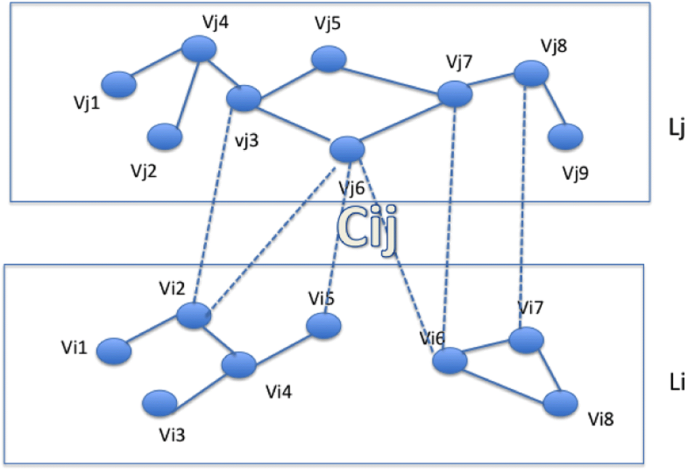
Example of a 2-layers network
-
2.
\(\mathbb {E}=\{E_{1},..E_{i},.. E_{l}\}\) is the set of edges intra-layer: Ei is a set of edges in layer number i, we denote ∣Ei∣ by mi. \(E_{i}=\{(v^{i}_{j}, v^{i}_{k})\mid v^{i}_{j} \in V_{i}, v^{i}_{k} \in V_{i} \}\)Footnote 1
-
3.
\(\mathbb {C}=\{ C_{i_{1}j_{1}},.. C_{i_{b}j_{b}} \mid i_{k } \neq j_{k }\}\) is the set of inter-layer links, b is the number of bipartite components. \(C_{{ij}}=\{(v^{i}_{k},v^{j}_{k'}) \mid v^{i}_{k} \in V_{i}, v^{j}_{k'} \in V_{j}\}\), we denote ∣Cij∣ by cij.

This representation allows to propose an adaptation of global and local metrics taking into account the intra-layers and the inter-layer links. We can then aggregate these metrics in order to propose a metric for the whole network. For example, we can propose the following metric for the density:
-
Intra-layer density for the layer i: \(D_{i}= \frac {m_{i}}{\frac {n_{i}* (n_{i}-1)}{2}}\)
-
Inter-layer density for the bipartite component Cij:
\(D_{{ij}}= \frac {c_{{ij}}}{n_{i}* n_{j}}\)
-
Multilayer density: \(D= \frac {\sum _{C_{{ij}} \in \mathbb {C}}{c_{{ij}}}+\sum _{l \in \{1..l\}}{m_{l}}}{\sum _{C_{{ij}} \in \mathbb {C}}{n_{i}* n_{j}}+ \sum _{l \in \{1..l\}}\frac {n_{i}* (n_{i}-1)}{2}}\)
Likewise, the degree centrality can be generalised to the inter-layer level and to the whole networks. The centrality degree and connectivities of a vertex \(v^{i}_{j}\) belonging to the layer Vi are given by:
-
Intra-layers degree: \(CD\left (v^{i}_{j}\right)=\frac {deg_{i}(v^{i}_{j})}{n_{i}-1}\) where ni=∣Vi∣ where \(deg_{i}\left (v^{i}_{j}\right)\) is the degree of \(v^{i}_{k}\) in the layer i.
-
Inter-layers connectivity: we define the connectivity of a vertex in the bipartite component Cik as \(CN_{k}\left (v^{i}_{j}\right)=\frac {deg_{C_{{ik}}}(v^{i}_{k})}{n_{k}}\) where nk=∣Vk∣ and \(deg_{C_{{ik}}}\left (v^{i}_{k}\right)\) is the degree of \(v^{i}_{k}\) in Cik
-
Multilayers connectivity: we propose to generalise the definition of the connectivity of a node to the whole network: \(CN\left (v^{i}_{j}\right)=\frac {deg_{i}(v^{i}_{j}) + \sum _{k}{CN_{k}(v^{i}_{j})}}{{n_{i}-1} + \sum _{k}{n_{k}}} \mid {C_{{ik}} \in \mathbb {C}}\),
Multilayer egocentric networks
Given a complex network (and more particularly an online social network), the egocentric network is defined around an ego node u is a sub-network containing the ego u and the alters (the neighbours) as well as the set of links of the ego-network. In the literature, two cases of online personal networks are identified depending on the distance of the alters from the ego: 1-level and k-level.
Let G=(V,E), and u a vertex, the 1-level egocentric network of u Gu=(Vu,Eu) is given by (see Fig. 2) :
-
Vu={x∈V∣(u,v)∈E}∪{u}
Fig. 2 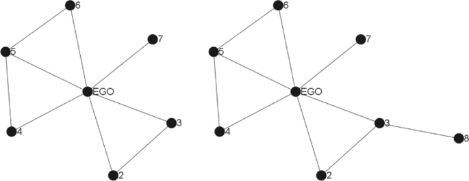
1-level and 2-level ego-networks
-
Eu={(x,y)∈E∣x∈Vu∧y∈Vu}

We propose an extension of this definition to multilayer networks which aims to access to the alters located in the same layer as well as the layers connected to the one of the ego (see Fig. 3).

Example of a 2-layers egocentric network
u∈Vi, \(\mathbb {N}^{u}=G(V^{u},E^{u})\)
-
Vu={x∈Vi∣(u,x)∈E}∪{u}∪k{y∈Vk∣(u,y)∈Cik}
-
Eu={(x,y)∈Ei∣x∈Vu∧y∈Vu}∪k{(u,y)∈Cik}
Private multilayer network and private egocentric network
As mentioned before the purpose of this study is to provide domain experts with measures and methods to understand, evaluate and complete their private data by comparing and/or combining them with open data when both are modelled by multilayer networks. In our case, private data is a subset of nodes that are identified in the open network. The interactions between these private nodes are extracted for the open network We therefore propose to study the induced graph elaborated from the private data. This one has to be constructed, analysed and compared to the whole (open) network (see Fig. 4).

Multilayer network and private data: blue graph represents the open network, red nodes (on the left) are private data. Red graph (on the right) represents the private network
Let \(\mathbb {N} \) be a multilayer network (extracted form the open data) : \(\mathbb {N}=(\mathbb {V},\mathbb {E},\mathbb {C})\) containing l layers. Let PV be a set of vertices PV={PV1,..PVl} such that : PVi⊂Vi (private data). We define the private multilayer Network \(\mathbb {N}[PV]=(\mathbb {PV},\mathbb {PE},\mathbb {PC})\) where
-
1.
\(\mathbb {PE}=\{PE_{1},..PE_{i},.. PE_{l}\}\) is the set of intra-layers edges:
PEi is the set of edges in the layer number i given by: \(PE_{i}=\left \{\left (pv^{i}_{j}, pv^{i}_{k}\right) \in E_{i} \mid pv^{i}_{j} \in PV_{i}, pv^{i}_{k} \in PV_{i} \right \}\)
-
2.
\(\mathbb {PC}=\left \{ PC_{i_{1}j_{1}},.. PC_{i_{b}j_{b}} \mid i_{k } \neq j_{k }\right \}\) is the set of inter-layer links
\(PC_{{ij}}=\left \{\left (pv^{i}_{k},pv^{j}_{k'}\right) \in C_{{ij}}\mid pv^{i}_{k} \in PV_{i}, pv^{j}_{k'} \in PV_{j}\right \}\).
In Fig. 4, the blue graph represented the multilayer network \(\mathbb {N} \) extracted from the open data, red nodes represent the private data and the red graph illustrates the private multilayer network \(\mathbb {N}[PV]\).
We extend now the definition of egocentric network (which is defined around a given ego node (Marsden 2002; Djemili et al. 2017)) to an egocentric network around private multilayer network.
We define the private egocentric network as follow:
Let \(\mathbb {N}[PV]=(\mathbb {PV},\mathbb {PE},\mathbb {PC})\) be the private mutilayer network. We define the private egocentric network : \(\mathbb {N}^{PV}=G\left (V^{PV},E^{PV}\right)\)
-
\(V^{PV}= \bigcup _{u \in PV} \{x \in V_{i} \mid (u,x) \in E_{i}\} \bigcup \{u\}\bigcup _{k} \{y \in V_{k} \mid (u,y) \in C_{{ik}} \mid {C_{{ik}} \in \mathbb {C}}\}\)
-
\(E^{PV}=\bigcup _{u \in PV}\{(x,y) \in E_{i} \mid x \in V^{u} \wedge y \in V^{u} \}\bigcup _{k} \{(u,y) \in C_{{ik}} \mid {C_{{ik}} \in \mathbb {C}}\}\)
In Fig. 5, red nodes represent the private data and the graph containing red and yellow nodes and edges illustrates the private egocentric network \(\mathbb {N}^{PV}\)

Multilayer complex network: private egocentric network is represented by red and yellow nodes and edges
Layer and inter-layer reachability of a subnetwork
We define a graph reachability for a given layer as follow:
Let \(\mathbb {N}=(\mathbb {V},\mathbb {E},\mathbb {C})\) be a multilayer network containing l layers, G=(V,E) a subgraph of \(\mathbb {N}\) and i a given layer.
-
Reachability(G,i) is given by the subgraph \(\phantom {\dot {i}\!}G_{i}=(V{\prime }_{i},E{\prime }_{i})\):
-
\(\phantom {\dot {i}\!}V^{\prime }_{i}=\{v{\prime }^{i}_{j} \in V \cap V_{i}\}\)
-
\(\phantom {\dot {i}\!}E^{\prime }_{i}=\left \{\left (v{\prime }^{i}_{j}, v{\prime }^{i}_{k}\right) \in E \cap E_{i}\right \}\)
-
In order to appreciate the connection strength between private nodes across layer, we apply the reachability on the private egocentric network computed on a given layer i to another layer j. Let \(\mathbb {N}^{PV_{i}}=G\left (V^{PV_{i}},E^{PV_{I}}\right)\) be the private egocentric network computed from the layer i, let the reachability \(Reachability\left (\mathbb {N}^{PV_{i}},j\right)\) to another layer j be the graph \(\phantom {\dot {i}\!}\mathbb {N}{\prime }^{PV_{i}}_{j}\). Let \(V^{\prime }_{j}\) be the set of nodes of \(\phantom {\dot {i}\!}\mathbb {N}{\prime }^{PV_{i}}_{j}\), we can now evaluate the ratio of reachable private nodes on layer j by computing the precision and the recall as follow (see Figs. 6 and 7):

Reachability from layer i to layer j: red nodes are private ones, yellow and orange nodes are egocentrics ones computed from layer i, green nodes are the egocentric ones that belong to the the private network of the layer j, precisionR(i,j)=1 and recallR(i,j)=0.4: this means that all reachable nodes from layer i are private ones but only 40% of private nodes of the layer j are reachable from layer i

Reachability from layer j to layer i: red nodes are private ones, yellow and orange nodes are egocentrics ones computed from layer j, green nodes are the egocentric ones that belong to the the private network of the layer i, precisionR(j,i)=0.5 and recallR(j,i)=1: this means that 50% of reachable nodes from layer j are private ones but all private nodes of the layer i are reachable from layer j
precisionR(i,j) gives the ratio of private nodes belonging to layer j that are reachable from layer i to all reachable nodes in the layer j. recallR(i,j) is the ratio of private nodes of the layer j that are reachable from layer i to all private nodes belonging to layer j.
We define also a graph inter-layer reachability for a given bipartite part as follow. Let \(\mathbb {N}=(\mathbb {V},\mathbb {E},\mathbb {C})\) be a multilayer network containing l layers, G=(V,E) a subgraph of \(\mathbb {N}\) and Cij is a given bipartie part.
-
InterReachability(G,Cij) is given by the subgraph \(\phantom {\dot {i}\!}G_{{ij}}=(V{\prime }_{{ij}},E{\prime }_{{ij}})\)
-
\(\phantom {\dot {i}\!}V^{\prime }_{{ij}}=\left \{v{\prime }^{i}_{k} \in V \cap V_{i} \right \} \cup \left \{v{\prime }^{i}_{k^{'}} \in V \cap V_{j}\right \}\)
-
\(\phantom {\dot {i}\!}E^{\prime }_{{ij}}=\left \{\left (v{\prime }^{i}_{k}, v{\prime }^{j}_{k^{'}}\right) \in E \cap C_{{ij}}\right \}\)
-
Given a bipartite part Cij, we can apply the InterReachability from the private induced multilayer network or from the private egocentric one.
For example, let \(\mathbb {N}[PV]\) be the private multilayer network, let \(InterReachability(\mathbb {N}[PV],C_{i j})\) be the graph \(C^{\prime }_{{ij}}\) we can evaluate the reachable bipartite edges by computing the ratio \(\frac {c{\prime }_{{ij}}}{c_{{ij}}}\) where \(c^{\prime }_{{ij}}= \mid C{\prime }_{{ij}} \mid \) and cij=∣Cij∣
Related work
Recently, there have been increasingly intense efforts to investigate networks with multiple types of connections as well as the so-called “networks of networks”. Variants of such systems have been examined decades ago in disciplines such sociology and engineering, but only recently have they been unified, along with other nomenclature, within the framework of multilayer networks defined by Kivelä et al.
In Kivelä et al. (2014) a complete review of the field of multilayer network is presented, the networks types, the characteristics of nodes and layers, the notion of aspect as well as the nature of coupling between layers are detailed.
Many studies are currently addressing themes related to multilayer networks as structure and dynamics of multilayer networks (Boccaletti et al. 2014; Magnani and Rossi 2013; Aleta and Moreno 2019), communities detection in multilayer networks (Liu et al. 2018) and visualisation (Mcgee et al. 2019).
Many work show also that experts in multiple domains as digital humanities (McGee et al. 2016), biology (Gosak et al. 2017), techno-anthropology etc. present their data using the multilayer networks and are aware of the strong necessity of having tools that analyse their data (Kivelä et al. 2019).
In this paper, we propose a methodology for multilayer network analysis in order to provide domain experts with measures and methods to understand, evaluate and complete their private data by comparing and/or combining them with open data when both are modelled as multilayer networks.
This methodology uses a formalism based on a set of graphs some of them represent layers (see “Notations, properties and metrics” section), others are biparties graphs representing the inter-layers connections. This formalism allows us to clearly separate three types of analysis: the intra-level one, the inter-level one and the global one that aggregate both (intra and inter) levels.
In Kivelä et al. (2014), a general formalism of the most general type of multilayer network was proposed, an underlying graph that represents this multilayer network is defined, where a node is represented by a tuple containing three identifiers: the node one, the layer one and the aspect one. In addition, two types of edges are proposed: intra-layer edges and inter-layer ones.
Our formalism for multilayer network allows to carry out fine analysis by considering two levels (see “Notations, properties and metrics” section) : the intra-layer level and the inter-layer one. We showed above, examples of how we can extend the definition of global and local measures as density and centralities to the inter-layer level. Measures for the whole networks are then computed by aggregating both precedent measures.
In many other work (Battiston et al. 2014), a monoplex network is constructed by aggregating data from the different layers of a multilayer network, the classical definition of node degree is then applied to the resulting monoplex network. However, network aggregation leads to a loss of information. In Some other work, the distinction of the layers is maintained and the degree of node is represented by a vector. It is also possible to define degree and neighbourhood in terms of a focal node and any subset of the layers (Berlingerio et al. 2013).
On the other hand, we defined layer and inter-layer reachability metrics of a given sub-network this measure is based on the private egocentric network and help to appreciate the connectivity strength of private data across layers (see “Layer and inter-layer reachability of a subnetwork” section).
In Kivelä et al. (2014) the mesure of node interdependence is defined as being the ratio of shortest paths in which two or more layers are used to the total number of shortest paths. It is a measure to quantify the value added by the multiplexicity to the reachability of nodes. The interdependence of a multiplex is computed as the average node interdependence.
Biological application
The aim of this application is to study several sets of biological data collected in experimentally related samples (i.e. cannabis samples). Identified molecules (proteins and metabolites) are measured form the biological collected data in different “omics” experiments: transcriptomics, proteomics and metabolomics. In their experiments, biologist measured at several time points, contigs: each one quantify genes, spots: each one quantify one or more proteins, and metabolites. Each gene produce typically one protein but sometimes more proteins.
At this point we only have nodes (but no edges), corresponding to molecules measured in the experiments. To get relationships biologist frequently used the open STRING (Search Tool for the Retrieval of Interacting Genes/Proteins) database (Szklarczyk et al. 2019), which is the main protein-protein (and so also gene-gene) interactions database as well as the STITCH (Search Tool for InTeractions of CHemicals) one. STITCH (Szklarczyk et al. 2016) is a twin database including edges between metabolites and metabolites, and also between proteins and metabolites (see Fig. 8). Each interaction in both databases is based on the presence of experimental, coexpression (similar behaviour across several public available experiment), text mining (appearing in the same phrase),pathway (participating to the same known biological network). A combined score aggregating all these types of interactions whose value is are between 0 and 1000 is added to both databases (see Tables 1, 2 and 3).

The network construction from the open databases: Protein-protein interactions are extracted from the STRING database. Metabolite-metabolite and metabolite-protein ones are extracted from the STITCH database
The open multilayer network is constructed form the open STRING and STITCH databases (see Fig. 8). Weighted interactions (edges) between proteins-proteins, metabolites-metabolites and proteins-metabolites are created according to the value of the combined score. The private data is the set of identified proteins and metabolites collected experimentally in the laboratory by biologists as mentioned above and will present a set of nodes in the whole open data as explained in Fig. 4.
Once the regulatory network has been sketched, it shall be analysed. The complexity of the network shall be reduced, by selecting significant interactions. Biologists need to identify key nodes (molecules) shortest paths, sort them via centrality measures between given ends and track the path from a receptor to transcription factors and vice versa.
From a biological point of view we remind that:
-
1.
Biologists are often interested to find neighbours of molecules (and more particularity proteins), hence the necessity to analyse the private egocentric network.
-
2.
Biologists need to extract and analyse signal transduction and metabolic pathways from the network. Shortest path is biologically meaningful as energetically the most favorable for detecting the signal transduction interactions as well as the metabolic pathways.
Signal transduction represent a series of interactions between different bioentities such as proteins, chemicals or macromolecules in order to investigate how signal transmission is performed either from the outside to the inside of the cell, or within the cell.
Likewise, metabolic pathways are related to a series of chemical reactions occurring within a cell at different time points holding information about a series of biochemical events and the way they are correlated we consider.
To analyse the biological network we proceed as follow:
-
1.
Analysis of each layer (proteins and metabolites layers)
-
(a)
The layer is constructed from the open data base (STRING and STITCH). Private network is also constructed from the set of identified molecules (proteins and metabolites) collected from the cannabis samples experiment, where biological data are collected in different “omics” experiments: transcriptomics, proteomics and metabolomics.
-
(b)
Global and local measures are compared and discussed for open and private networks, we apply the Louvain algorithm (Blondel et al. 2008) in order to detect communities, private (identified from experiment) molecules distribution is studied according to the detected communities.
-
(a)
-
2.
Multi-layer network analysis:
-
(a)
The bipartite component containing the interactions proteins-metabolites is constructed from the open STITCH data base. The whole multilayer networks, the private multilayer network as well as the private egocentric networks are also constructed.
-
(b)
Networks global and local measures are compared and discussed.
-
(c)
Layer reachablities from metabolites to proteins and from proteins to metabolites are computed and discussed.
-
(d)
Shortest paths between pairs of private proteins are then analysed and classified according to their location in the open network (private, egocentric or extra-egocentric). The KEGG open data set (Kanehisa and Goto 2000) is also used to describe pathways.
-
(a)
Open biological databases are very big in relation to the average high throughput biological experiment. In our case the proteins in the experiment represent only form 0.58% to 0.74% of the total number of proteins in the whole network. The metabolites in the experiment represent less than 0.05% of the total number of metabolites in the whole network.
Proteins layer analysis
Table 4 shows the distribution of the combined score values. Combined scores express strength interactions between two proteins according to the open STRING database.
Figure 9 shows that the distribution of the values of the combined scores is similar to scale free network behaviour.
-
1.
Network construction We construct the proteins layer by considering the combined score as threshold: if we take the minimum score (150) all the interactions are considered otherwise a part of the network is considered according the chosen percentile (see Fig. 10). When the combined core value is incremented some nodes will be disconnected. These nodes are dropped from the network. The private network is constructed also. (see Appendix A for more details)
Fig. 9 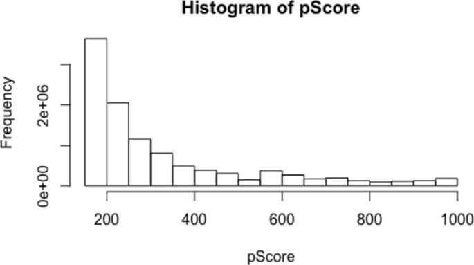
The distribution of the combined score extracted from the open STRING data base
Fig. 10 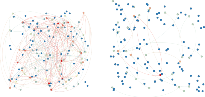
Private proteins networks: the left one corresponds to the minimum combined score (150), the right one corresponds score values greater than 500. Warm colours for nodes indicate hight degree centralities. Warm colours for edges indicate hight weights
Identified proteins in the experiment present only form 0.58% to 0.74% from the total number of proteins in the open network (see Table 5).
Table 5 Proteins layer analysis: summary of results for the minimum combing score Network densities do not vary a lot between the open and the private networks which means that the identified proteins (in the experiment) are almost balanced distributed in the whole protein layer.
We notice also that from the 75th percentile, certain identified proteins begin to be missed (see Appendix A for more details).
-
2.
Degree distribution:
Results show that the degrees centralities mean values of the identified proteins do not vary a lot in comparison to the other proteins (see Appendix A for more details). This is coherent with the observation on the networks densities that we mention above (see Table 5).
-
3.
Communities detection: We apply the Louvain algorithm to the protein layerFootnote 2 (Blondel et al. 2008). Eight communities are detected for the minimum score. We notice that the values of the precision in all communities are not varying a lot (see Appendix A for more details). This means that the identified proteins are almost distributed in a balanced way in communities.


Table 5 shows a summary of results and observations concerning the protein layer analysis.
Metabolites layer analysis
Table 6 shows the distribution of combined scores values. Combined scores express the strength of the interaction between two metabolites according to the STITCH data base.
Figure 11 shows that the distribution of the values of the combined sore is similar to scale free network behaviour.
-
1.
Network construction As for proteins layer, we construct the metabolites layer by considering the combined score as threshold, if we take the minimum score (2) the whole network is constructed networks otherwise a part of the network is considered according the chosen percentile (see Fig. 12).
Fig. 11 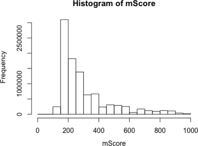
The distribution of the combined score extracted from the open STITCH data base
Fig. 12 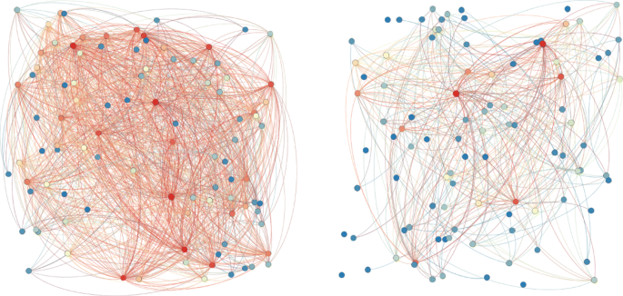
Private metabolites networks: the left one corresponds to the minimum combined score (2), the right one corresponds to score values greater than 500. Warm colours for nodes indicate hight degree centralities. Warm colours for edges indicate hight weights
We notice that the identified metabolites in the experiment present less than 0.05% from the total number of metabolites in the whole network. However the private metabolites networks extracted form the experiment present high density in comparison with the open ones (see Appendix B for more details).This means that the metabolites of the experiment are highly connected by pairs (see Table 7).
Table 7 Metabolites layer analysis: summary of results for the minimum combing score -
2.
Degree distribution:
Results show that the identified metabolites have very high degree centralities (see Appendix B for more details). This means they are strongly connected connected by pairs according to the STITCH open data base (see Table 7).
-
3.
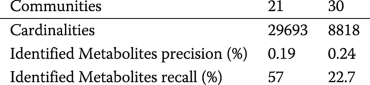
Communities detection : We apply the Louvain algorithm to the metabolites layer (Blondel et al. 2008), we obtain a modularity of is 0.46. 39 communities are detected from the principal connected component for the minimum combined score (see Appendix B):
-
22 have their cardinalities between 3 and 28
-
11 have their cardinalities between 1000 and 10000
-
6 have their cardinalities between 15000 and 30000
We notice that a majority of the metabolites are present in only two communities. This results is correlated with the high density value of the private metabolite network and means that metabolites are strongly connected and forms mainly two highly connected subnetworks.
-


Table 7 shows a summary of results and observations concerning the metabolites layer analysis.
Proteins-metabolites network analysis
Figure 13 shows that the distribution of the values of the combined scores extracted from the STITCH data base is similar to scale free network behaviour.
-
1.
Networks construction: We construct the protein-metabolite bipartite part by considering the combined score as threshold, if we take the minimum score the whole network is constructed otherwise a part of the network is considered according the chosen percentile. The 2-layer network is then constructed by considering the proteins and the metabolites layers. The private 2-layers network extracted from the experiment as well the private egocentric one are also constructed.
Results (see Appendix C) show that:
-
The ratio of identified molecules (proteins and metabolites) in the experiment is 0.1% compared to the open 2-layers networks but decreases to [0.9%, 1.42%] in the private egocentric network.
-
the density of the private networks obtained from the experiment is 100 to 165 bigger that the one of the open network but it is only 1,65 bigger than the one of egocentric network.
-
-
2.
Proteins and metabolites reachabilities: Table 8 shows that private egocentric metabolites networks reaches (see “Layer and inter-layer reachability of a subnetwork” section) a set of proteins that contains 51% to 67% of the identified proteins despite a very low precision.
Likewise, Table 9) shows that private egocentric proteins networks reaches (see “Layer and inter-layer reachability of a subnetwork” section) a set of metabolites that contains 53% to 84% of the identified metabolites despite a very low precision.
These results show that a majority of identified metabolites (in the experiment) are reachable from all the identified proteins and vice-versa. This will help biologist to classify molecules into neighbours ones and distant ones.

The distribution of the combined score extracted from the open STITCH data base
We present in next sections two methods for proteins pathway analysis: the first one is based on analysing the shortest paths between pairs of private proteins and the second one is based on using the affiliation network extracted from the open KEGG Database (Kanehisa and Goto 2000).
Proteins pathways analysis using shortest paths
shortest path is biologically meaningful as energetically the most favorable. The private protein networks is composed of 142 proteins (see Table 16, shortest paths are computed between 20164 pairs of proteins. Table 10 shows the number and percentage of shortest paths classified by theirs lengths
We can thus propose a classification of the obtained shortest paths into three classes according to their location in the whole proteins networks :
-
1.
Shortest paths whose lengths are less than or equal two: these pathways belong to the private protein network.
-
2.
Shortest paths whose lengths are less than or equal four: these ones can either reach the egocentric networks or belong completely to the private one.
-
3.
Shortest paths whose lengths are more than four: these ones can either reach the open networks, or belong completely to the egocentric or the private one
We notice that the majority of found shortest paths belong to the egocentric network (or the private one) so they are in the neighbours of the private network nodes. Only few of them (3,37 %) can be outside the egocentric networks. These few long shortest paths can be isolated and studied by biologists in order to understand the molecule interactions into these paths. Table 11 shows two shortest paths pf length 6 composed of proteins and metabolites: one have some nodes outside the egocentric network and the other one is completely inside the egocentric network and the other one
Proteins pathways analysis using the KEGG data base
KEGG (Kyoto Encyclopedia of Genes and Genomes) is an open database resource that integrates genomic, chemical and systemic functional information. In particular, gene catalogs from completely sequenced genomes are linked to higher-level systemic functions of the cell, the organism and the ecosystem (Kanehisa and Goto 2000).
Major efforts have been undertaken to manually create a knowledge base for such systemic functions by capturing and organising experimental knowledge in computable forms; namely, in the forms of molecular networks called KEGG pathway maps, BRITE functional hierarchies and KEGG modules.
From the KEGG data set we extract 4692 proteins which are associated to Pathway identifiers. Each identifier is also related to a pathway name that characterised the molecules (see Tables 12 and 13). There are 238 pathways.
Our goal is to use this data set in order to characterise the set of private proteins extracted from the experiment. We represent the affiliation of private proteins by an affiliation network extracted from the KEGG database and modelled by a bipartite graph containing the set of private proteins connected to pathway identifiers (see Fig. 14). Bipartite networks are a particular class of complex networks, whose nodes are divided into two sets X and Y, and only connections between two nodes in different sets are allowed. Bipartite networks can usually be compressed by one-mode projection. This means that the ensuing network contains nodes of only either of the two sets, X (or, alternatively, Y) nodes are connected only if when they have at least one common neighbouring Y (or, alternatively, X) node (see Fig. 15).

The private affiliation network extracted from the KEGG database: private proteins connected to pathway identifiers

Illustration of the one-mode projection form a bipartite network
We consider the pathway networks obtained by one-mode projection on the pathways set. Table 14 shows the characteristics of this network.
In order to characterise the private proteins data set we proceed as follow: we firstly apply the Louvain algorithm (Blondel et al. 2008) to the pathway on-mode projection network in order to detect communities. Pathways that belong to the same community are similar in the the sens that they are associated to some proteins in commun.
We then analyse the pathways of the private proteins set in comparison with each community. Let PathE be the set of pathways associated to the private proteins. Let PathCi be the set of pathways included in the community number i. For each community i we compute
-
1.
The experiment precision given by \(\frac {PathC_{i} \cap PathE}{PathC_{i}}\): measures the rate of private proteins pathways among the pathways included in the community.
-
2.
The experiment recall given by \(\frac {PathC_{i} \cap PathE}{PathE}\): measures the rate of private proteins pathways among all the private proteins pathways.
-
3.
The jaccard Index given by \(\frac {PathC_{i} \cap PathE}{PathC_{i} \cup PathC_{i}}\): measures the rate of private proteins included in this community and that have an affiliation
Table 15 shows results concerning the found communities, some of them correspond to isolated pathways (of cardinality one) that do not have private proteins affiliation (experiment precision is equal to 0) or that have isolated affiliation (experiment precision is 1).
Each community can be described by a set of pathway names (see Table 13). The community 9 have the better Jaccard index with the set of private proteins. It has the following pathways description :["Oxidative phosphorylation", "N-Glycan biosynthesis", "Porphyrin and chlorophyll metabolism","Ribosome biogenesis in eukaryotes", "RNA transport","RNA degradation" “Spliceosome”, “Ubiquitin mediated proteolysis”, “Protein processing in endoplasmic reticulum”, “Circadian rhythm”]
We aim to study these pathways in order to show if the list of metabolites and proteins found on the pathways are biologically significant. We aim also to compare them to shortest paths and their relations to the private egocentric network.
Results discussion
We discuss in this section results obtained from the application of our methodology to the above biological application. We present observations and results related to one layer and those obtained for the whole network.
Observations and results obtained from one layer analysis
Our analysis methodology allows biologists to compare and assess identified molecules and private networks with the open ones as described follows (see Tables 5 and 7):
-
Firstly, the rate of the identified molecules is computed in relation to the open network. This helps biologists to position the identified molecules in comparison with the open data. In our case, open biological databases are very big in relation to the average high throughput biological experiment. The proteins in the experiment represent only form 0.58% to 0.74% of the total number of proteins in the whole network. The metabolites in the experiment represent less than 0.05% of the total number of metabolites in the whole network.
-
The open and private networks’ densities measures are computed and compared, this gives an indication about the strengths of connections in the set of identified molecules in comparison with the open data. In our case, we notice that the open and the private proteins networks have almost the same density, on the other hand, the private metabolites network have high density in comparison with the open one.
-
The average degrees are computed for three set of nodes: the average degree of the open network, the average degree of the private one and the one for the set of identified molecules in the open one. Comparing these values helps biologists to appreciate the strength of connections between the identified molecules and all the other molecules in comparison with the strength of connection between all the molecules. In our case, degree values of identified proteins do not vary a lot in comparison to other proteins. On the other hand, identified metabolites have very high degree centralities, this means they are strongly connected to other metabolites (see Tables 5 and 7).
-
In order to have an idea about the distribution of the identified molecules in the network, we apply the Louvain algorithm (Blondel et al. 2008) in order to detect communities, private molecules (identified from experiment) distribution is studied according to the detected communities. In our case, eight communities are detected for the protein layer. The rate of distribution of identified proteins in these communities is ∈[0,48%;0,77%], this means Identified proteins are almost distributed in a balanced way in communities. Notice that theses rates is comparable to the global rate of identified proteins in the one network. On the other hand, 39 communities are detected for the metabolite layer. 80% of the identified metabolites belong only to 2 communities, this means that a majority of the Identified metabolites are strongly connected and forms two highly connected subnetworks. Biologists have confirmed these results by identifying two known categories of metabolites (see Tables 5 and 7).
Observations and results obtained from two layers analysis
-
The computation of layer reachablities from metabolites to proteins and from proteins to metabolites allow biologists to appreciate the ratio of immediate interactions between private molecules (identified in their experience) in comparison with the open data. Table 8 shows that private egocentric metabolites networks reaches (see “Layer and inter-layer reachability of a subnetwork” section) a set of proteins that contains 51% to 67% of the identified proteins despite a very low precision (0.6% to 0.64%).
Likewise, Table 9) shows that private egocentric proteins networks reaches (see “Layer and inter-layer reachability of a subnetwork” section) a set of metabolites that contains 53% to 84% of the identified metabolites despite a very low precision (0.56% to 0.7%).
-
Analysing shortest paths which are biologically meaningful between pairs of private proteins could be very helpful for biologists. We propose to classify them according to their location in the open network (private, egocentric or extra-egocentric). In our case, we notice that the majority of found shortest paths belong to the egocentric network (or the private one) so they are in the neighbours of the private network nodes. Only few of them (3,37 %) can be outside the egocentric networks. These few long shortest paths can be isolated and studied by biologists in order to understand the molecule interactions into these paths.
-
By using the KEGG database (Kanehisa and Goto 2000), we proposed to characterise the set of private proteins identified from the experiment by pathways description presented as a list of pathway names. We aim to study these pathways in order to show if the list of metabolites and proteins found on the pathways are biologically significant. We aim also to compare them to found shortest paths and their relations to the private egocentric network.
Conclusion and perspectives
We presented in this paper a methodology including measures and methods which helps domain experts to understand, evaluate and complete their private data by comparing and/or combining them with open data, when both are modelled by multilayer networks.
We proposed a new formalism for multilayer network that allows to carry out fine analysis by considering two levels: the intra-layer level and the inter-layer one.
We introduced the notions of private multilayer network and private egocentric network which is defined around the private multilayer network. The private egocentric network is used to evaluate the connectivity strength between the different layers of private data in comparison to the open network. We showed how we can use these notions to define the layer and inter-layer reachability metrics of a given sub-network.
We illustrated our methodology through a biological application where interactions between molecules (proteins and metabolites) are extracted from open databases and modelled by a multilayer network. The private data is a set of proteins and metabolites collected experimentally and presented a set of nodes in the whole multilayer network. Current experimental results are relevant from biologists point of view.
We showed that the application of this methodology allows biologists to compare and assess identified molecules and private networks with the open one.
Computing open and private networks mesures for the different layers and as densities and degrees helps biologists to appreciate the strength of internal connections between the identified molecules and to compare with the one of connections to other molecules as well as to the global measures. Likewise, applying communities detection algorithms in the different layers gives an idea about the distribution of the identified molecules in the open network. Computing reachablities across layers (from metabolites to proteins and from proteins to metabolites) helps to appreciate the ratio of immediate interactions between private molecules as well as the set of open molecules reachable from the identified ones ; we remind that biologists are interested by finding neighbours of molecules and to make the distinction between those private and open. In addition, shortest paths which are biologically meaningful are also analysed and classified according to their location in the whole network (private, egocentric or extra-egocentric ones). The KEGG open data set (Kanehisa and Goto 2000) is also used to describe pathways.
We are currently working on communities detection (Fortunato 2010) across layer. We use layers and inter-layers reachabilities metrics in order to propose algorithm(s) allowing the comparisons and the mapping of communities across layers.
From a biological point of view, we aim to study which KEGG pathways are highlighted in order to show if the molecules connecting private ones are biologically significant. In such analysis we aim to compare: the list of metabolites and proteins found on the pathway, with all first neighbours, with the geocentric networks as well as with shortest paths.
Appendix A: Proteins layer analysis
-
1.
Network construction Table 16 shows global measures values of the open and experiment networks
-
2.
Degree distribution: Figure 16 shows the violin plots that allow to compare the degree distributions of the private protein networks.
Table 17 shows the degree distributions of the open network, of the identified nodes in the experimentation and of the private protein networks.
-
3.
Communities detection: Table 18 show the results of applying the Louvain algorithm to the protein layerFootnote 3 (Blondel et al. 2008). Eight communities are detected for the minimum score. We show the precision and recall values of the identified proteins from the experience for each community..

Degree distribution of the private proteins networks according to the chosen percentile
Appendix B: Metabolites layer analysis
-
1.
Network constructionTable 19 shows global measures values of the open networks as well as those of the private one.
-
2.
Degree distribution: Figure 17 shows the violin plots that allow to compare the degree distributions of the private metabolites networks.
Table 20 shows the degree distributions of the open network, the identified nodes in the experimentation as well as the private networks. We notice that the identified metabolites have very high degree centralities. This means they are strongly connected connected by pairs according to the STITCH open data base.
-
3.
Communities detection: We apply the Louvain algorithm to the metabolites layer (Blondel et al. 2008), we obtain a modularity of is 0.46. 39 communities are detected from the principal connected component for the minimum combined score:
-
22 have their cardinalities between 3 and 28
-
11 have their cardinalities between 1000 and 10000
-
6 have their cardinalities between 15000 and 30000
Table 18 Communities detection with the Louvain algorithm, Modularity is 0.38 We show in Table 3 the distribution of the main identified metabolites.
Table 19 Global measures values of the metabolites networks extracted from the STITCH database and the private networks according to combined score percentiles Fig. 17 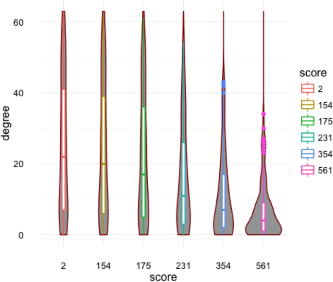
Degree distribution of the private metabolites networks according to the chosen percentile
-


Appendix C: Proteins-metabolites network analysis
-
Networks construction: Table 21 shows global measures values of the bipartite component, the whole networks, the private one and the private egocentric network according to combined score percentiles.
Notes
An edge is defined by (v,u) for directed graph respectively {v,u} for undirected graph
we consider the principal connected component of networks
we consider the principal connected component of networks
Abbreviations
- KEGG:
-
Kyoto encyclopedia of genes and genomes
- STRING:
-
Search tool for the retrieval of interacting genes/proteins
- STITCH:
-
Search tool for InTeractions of CHemicals
References
Aleta, A, Moreno Y (2019) Multilayer Networks in a Nutshell. Ann Rev Condens Matter Phys 10(1):45–62.
Ashburner, M, Ball CA, Blake JA, et al (2000) Gene ontology: tool for the unification of biology. The Gene Ontology Consortium. Nat Genet 25(1):25–29.
Battiston, F, Nicosia V, Latora V (2014) Structural measures for multiplex networks. Phys Rev E 89(3):032804.
Berlingerio, M, Coscia M, Giannotti F, Monreale A, Pedreschi D (2013) Multidimensional networks: foundations of structural analysis. World Wide Web 16(5-6):567–593.
Blondel, V, Guillaume J-L, Lambiotte R, Lefebvre E (2008) Fast unfolding of communities in large networks. J Stat Mech Theory Exp 2008(10). https://doi.org/10.1088/1742-5468/2008/10/p10008.
Boccaletti, S, Bianconi G, Criado R, CI Del Genio CI, et al (2014) The structure and dynamics of multilayer networks. Phys Rep 544(1):1–122.
Djemili, S, Marinica C, Malek M, Kotzinos D (2017) Personal Networks of Scientific Collaborators: A Large Scale Experimental Analysis of Their Evolution. Communications in Computer and Information Science, vol. 760. Springer, Cham.
Fortunato, S (2010) Community detection in graphs. Phys Rep 486:75–174.
Gosak, M, Markovic R, Dolensek J, Rupnik MS, Marhl M, Stozer A, Perc M (2017) Network science of biological systems at different scales: A review. Phys Life Rev. https://doi.org/10.1016/j.plrev.2017.11.003.
Kanehisa, M, Goto S (2000) KEGG: Kyoto Encyclopedia of Genes and Genomes. Nucleic Acids Res 28:27–30.
Kivelä, M, Arenas A, Barthelemy M, Gleeson JP, Moreno Y, Porter MA (2014) Multilayer networks. J Complex Netw 2(3):203–271.
Liu, W, Suzumura T, Ji H, Hu G (2018) Finding overlapping communities in multilayer networks. PLoS ONE 13(4). https://doi.org/10.1371/journal.pone.0188747.
Magnani, M, Rossi L (2013) Pareto distance for multi-layer network analysis, in Social Computing, Behavioral-Cultural Modeling and Prediction. Springer, Berlin. pp. 249–256.
Malek, M (2018) Private versus Open Multilayer Complex Networks, Data Science Workshop, Paris-Dauphine University, 22-23 January.
Marsden, PV (2002) Egocentric and Sociocentric Measures of Network M.E. Centrality. Soc Netw 24(4):407–422.
McGee, F, During M, Ghoniem M (2016) Towards visual analytics of multilayer graphs for digital cultural heritage In: 1st Workshop on Visualization for the Digital Humanities in IEEE VIS Conference, Baltimore.
Mcgee, F, Ghoniem M, Melançon G, Otjacques B, Pinaud B (2019) The State of the Art in Multilayer Network Visualization. Computer Graphics Forum. Wiley Online Library.
Newman, J (2003) The structure and function of complex networks. SIAM Rev 45(2):167–256.
Pavlopoulos, GA, et al (2011) Using graph theory to analyze biological networks. BioData Min 4.1:10. https://doi.org/10.1186/1756-0381-4-10.
Kivelä, M, McGee F, Melançon G, Henry Riche N, von Landesberger T (2019) Visual Analytics of Multilayer Networks Across Disciplines (Dagstuhl Seminar 19061). Dagstuhl Reports 9(2):1–26.
Szklarczyk, D, Gable AL, Lyon D, Junge A, Wyder S, Huerta-Cepas J, Simonovic M, Doncheva NT, Morris JH, Bork P, Jensen LJ, von Mering C (2019) STRING v11: protein-protein association networks with increased coverage, supporting functional discovery in genome-wide experimental datasets. Nucleic Acids Res 47:D607–613.
Szklarczyk, D, Santos A, von Mering C, Jensen LJ, Bork P, Kuhn M (2016) STITCH 5: augmenting protein-chemical interaction networks with tissue and affinity data. Nucleic Acids Res 44(D1):D380–4.
Acknowledgements
Not applicable.
Funding
This work was funded by the French ANR grant BLIZAAR ANR-15-CE23-0002-01 and the Luxembourgish FNR grant BLIZAAR INTER/ANR/14/9909176.
Author information
Authors and Affiliations
Contributions
MM proposed the methodology for multilayer networks analysis in the context of open and private data and was a major contributor in developing the prototype and writing the manuscript. SS was the major contributor concerning the biological application and more particularly for understanding and modelling the data as well as analysing and interpreting the results. MG had a major role in coordinating and managing the work, especially in the context of the BLIZAAR project. He also contributed to writing the manuscript. All authors read and approved the final manuscript.
Corresponding author
Ethics declarations
Competing interests
The authors declare that they have no competing interests.
Additional information
Publisher’s Note
Springer Nature remains neutral with regard to jurisdictional claims in published maps and institutional affiliations.
Rights and permissions
Open Access This article is licensed under a Creative Commons Attribution 4.0 International License, which permits use, sharing, adaptation, distribution and reproduction in any medium or format, as long as you give appropriate credit to the original author(s) and the source, provide a link to the Creative Commons licence, and indicate if changes were made. The images or other third party material in this article are included in the article’s Creative Commons licence, unless indicated otherwise in a credit line to the material. If material is not included in the article’s Creative Commons licence and your intended use is not permitted by statutory regulation or exceeds the permitted use, you will need to obtain permission directly from the copyright holder. To view a copy of this licence, visit http://creativecommons.org/licenses/by/4.0/.
About this article

Cite this article
Malek, M., Zorzan, S. & Ghoniem, M. A methodology for multilayer networks analysis in the context of open and private data: biological application. Appl Netw Sci 5, 41 (2020). https://doi.org/10.1007/s41109-020-00277-z
Received:
Accepted:
Published:
DOI: https://doi.org/10.1007/s41109-020-00277-z