Transformation of Infragravity Waves during Hurricane Overwash


1
Department of Civil and Environmental Engineering, Rice University, Houston, TX 77005, USA
2
Department of Ocean Engineering, Texas A&M University, Galveston, TX 77554, USA
3
Mediterranean Institute of Oceanography (MIO), Université de Toulon, Aix Marseille Université, CNRS, IRD, 83130 La Garde, France
4
Laboratoire des Sciences de l’Ingénieur Appliquées a la Méchanique et au Génie Electrique—Fédération IPRA, University of Pau & Pays Adour/E2S UPPA, Chaire HPC-Waves, EA4581, 64600 Anglet, France
5
Faculty of Civil Engineering and Geosciences, Environmental Fluid Mechanics Section, Delft University of Technology, 2628CN Delft, The Netherlands
*
Author to whom correspondence should be addressed.
†
Current address: Department of Geological Sciences, University of North Carolina at Chapel Hill, Chapel Hill, NC 27514, USA.
J. Mar. Sci. Eng. 2020, 8(8), 545; https://doi.org/10.3390/jmse8080545
Submission received: 1 July 2020
/
Accepted: 16 July 2020
/
Published: 22 July 2020
(This article belongs to the Special Issue Advances in Nearshore Hydrodynamics Research)
Abstract
:Infragravity (IG) waves are expected to contribute significantly to coastal flooding and sediment transport during hurricane overwash, yet the dynamics of these low-frequency waves during hurricane impact remain poorly documented and understood. This paper utilizes hydrodynamic measurements collected during Hurricane Harvey (2017) across a low-lying barrier-island cut (Texas, U.S.A.) during sea-to-bay directed flow (i.e., overwash). IG waves were observed to propagate across the island for a period of five hours, superimposed on and depth modulated by very-low frequency storm-driven variability in water level (5.6 min to 2.8 h periods). These sea-level anomalies are hypothesized to be meteotsunami initiated by tropical cyclone rainbands. Estimates of IG energy flux show that IG energy was largely reduced across the island (79–86%) and the magnitude of energy loss was greatest for the lowest-frequency IG waves (<0.01 Hz). Using multitaper bispectral analysis, it is shown that, during overwash, nonlinear triad interactions on the sea-side of the barrier island result in energy transfer from the low-frequency IG peak to bound harmonics at high IG frequencies (>0.01 Hz). Assuming this pattern of nonlinear energy exchange persists across the wide and downward sloping barrier-island cut, it likely contributes to the observed frequency-dependence of cross-barrier IG energy losses during this relatively low surge event (<1 m).
1. Introduction
During hurricanes, the nearshore environment extends landward as ocean water levels become elevated by storm surge and wave setup. Along barrier island lined coasts, ocean-to-bay directed flow can occur during hurricane-driven overwash and island inundation [1]. Due to a paucity of hydrodynamic observations during overwash and inundation [2,3,4,5,6,7], it is not well understood how the incident wave field transforms across long expanses of mild, sandy slopes characteristic of many barrier islands. Furthermore, no field studies to date have detailed wave transformation across barrier islands during hurricane impact. Insight into the role and duration of wave processes during overwash and inundation is essential for improving prediction of coastal flooding, beach and dune erosion, and impacts to coastal infrastructure.
On closed sandy beaches (no overwash and inundation), field observations show that infragravity (IG) waves (frequencies f nominally 0.003–0.04 Hz) can dominate shoreline water motions during energetic storm conditions. Whereas wave breaking limits the height of sea-swell waves (0.04–0.25 Hz) in the inner surf zone, IG waves can continue to grow in height close to shore with increasing offshore incident wave energy (e.g., [8,9,10,11,12]), in some locations reaching over 1 m in height [13,14,15,16]. Observations of energetic IG waves extend beyond the shoreline during storms. Recent field studies have shown that IG waves can propagate into lagoons during storm impact and contribute to tidal inlet morphodynamics [17,18,19]. Given the energetic behavior of IG waves both on closed beaches and in lagoon environments during storms, a general assumption of morphodynamic numerical models—while limited in field observations for validation—is that IG waves contribute significantly to morphological change during overwash and inundation (e.g., [20,21]), and consequently the generation of washover deposits [22].
Field observations from the few studies that have documented in-situ wave fields during storm-driven (non-hurricane) overwash [3,7] and inundation [6] have shown that IG waves can indeed dominate the incident wave field across barrier islands during coastal flooding. Wave measurements collected by Engelstad et al. [6] during inundation of a barrier island in the Netherlands show that IG waves can be onshore progressive and bore-like in shape as they propagate across long stretches of shallow water depths into back-barrier bays. Wave breaking was identified as the dominant energy dissipation mechanism (over frictional damping) for IG waves, particularly seaward of the berm crest. Previous field and laboratory studies of closed beaches have shown that IG waves not only dissipate energy through wave breaking (e.g., [15,16,23,24,25]) or bottom friction (e.g., [24,26,27]), but also lose energy to higher frequencies through nonlinear triad interactions in the shallow waters of the inner surf zone (e.g., [14,27,28,29,30,31,32]). Nonlinear energy transfers were not incorporated in the cross-barrier energy balance of Engelstad et al. [6]. Given that we know that nonlinear triad interactions play a large role in the spectral evolution of breaking surface gravity waves [33], and non-breaking IG waves in shallow water (e.g., [27]), it is likely that nonlinear energy transfer is also important in the shoaling and transformation of IG waves during overwash an inundation, and consequently the cross-barrier energy balance. However, analysis of nonlinear energy transfer during storm impact is challenging as traditional bispectral estimators require long, stationary wave records to achieve statistical significance.
Here, we present new observations of temporal and spatial trends in IG wave dynamics at two neighboring barrier islands along the Texas Gulf coast (Gulf of Mexico, U.S.A) during Hurricane Harvey (2017). Section 2 provides an overview of the study region, storm impacts, and field observations. Data processing techniques and methodology are outlined in Section 3. Prior to detailing IG wave transformation during island overwash (Section 4.2), a brief characterization of IG waves and discussion of potential generation mechanisms is provided using surf zone data from a closed beach farther up the coast (Section 4.1). It is shown that IG energy losses across a pre-existing and low-lying barrier-island cut during overwash—calculated for a range of water depths given uncertainties in bed level—are frequency dependent. In Section 5, we use multitaper bispectral analysis, a technique particularly well suited for short time series, to explore the potential role of nonlinear energy transfer in cross-barrier changes in IG energy and frequency content. The importance of episodic, very low frequency sea-level anomalies (0.1–3 mHz, 5.6 min to 2.8 h periods) on IG wave transformation during overwash is also discussed, as well as their hypothesized origin as meteotsunamis driven by tropical cyclone rainbands.
2. Field Observations
2.1. Study Sites
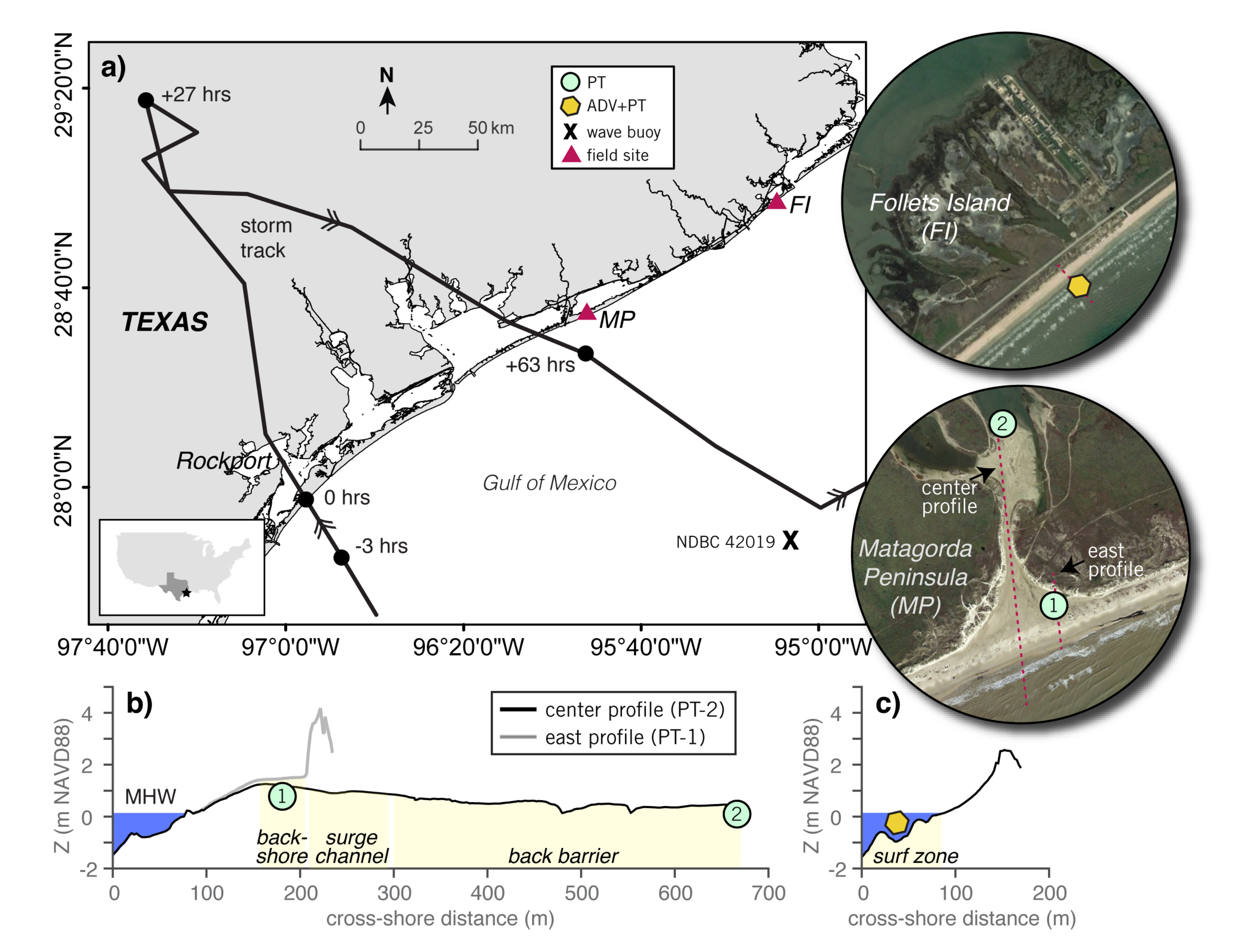
Matagorda Peninsula and Follets Island are retrogradational barrier islands [34] located on the central and upper portion of the Texas coast, respectively (Figure 1a). This region of the Gulf of Mexico (GOM) is a mixed semi-diurnal, micro-tidal (mean tidal range <0.5 m), wave-dominated environment with a prevailing longshore current toward the southwest [35]. Both barriers are long (35 km and 23 km, respectively), narrow (0.5 to 1.5 km), and low-lying (on average < 2 m high), which allows for frequent overwash during storms. The locations selected for instrument deployment straddle infilled surge channels (alternatively “barrier-island cuts”) and historical washover fans. The beaches at both field sites are low gradient (beach slope ≈ 0.017) with several pronounced bars and troughs composed of very fine to fine sand ( = 0.13–0.25 mm). A dune line separates the backshore from the back-barrier environments at both Matagorda Peninsula (Figure 1b) and Follets Island (Figure 1c).
2.2. Instrumentation
In advance of hurricane landfall, pressure transducers (PTs) were deployed on the ocean and bay side of both barrier islands, housed within shallow monitoring wells. At Matagorda Peninsula, PTs were installed in the backshore (PT-1) and ∼500 m down-slope in the back barrier (PT-2, Figure 1b), both environments that are typically subaerial during quiescent conditions. Following the methodology of Sherwood et al. [5], each PT was installed by jetting a 1.5 m-long schedule-80 PVC well to a depth of 1.3 m such that the well cap was elevated above the bed. The well casings were made permeable by narrow slits along the majority of their length. The PTs were fixed to an aluminum rod 0.20 m below the top of the well cap so to position the PT membrane at the elevation of the pre-storm bed and at the top of the slotted region (see Figure S1). Instrumentation at the Follets Island location included an acoustic Doppler velocimeter with a co-located PT (ADV+PT) deployed in the surf zone just seaward of the first sandbar (Figure 1c) and a PT installed ∼900 m landward in the back barrier (not discussed herein).
All instruments recorded continuously at 16 Hz (PT-1 and the ADV+PT) or 2 Hz (PT-2) enabling measurement of wave fields on either side of both barriers. The PTs measured water levels with a manufacturer-specified accuracy of 0.05% of full operating depth (1 cm) and resolution of 0.001% of full scale operational water depth (0.02 cm). Pre- and post-storm measurements of instrument elevations showed that all instruments stayed in place, albeit some small differences in GPS vertical elevations were observed at PT-1 and PT-2 (Figure S1). These differences are attributed to pre-storm GPS error as the post-storm positioning of the PTs agrees well with observations of pressure head (Section 2.4). Hence, in the discussion of storm impacts below, post-storm PT elevations are used to reference pressure head (i.e., where P is measured pressure corrected for atmospheric pressure, is water density, and g is gravitational acceleration) relative to North American Vertical Datum 1988 (NAVD88).
2.3. Overview of Storm Impacts
Hurricane Harvey made landfall as a Category 4 hurricane on 26 August 2017 at approximately 3:00 a.m. UTC near Rockport, Texas (Figure 1a). As the storm moved inland, the forward motion of the hurricane was greatly reduced and eventually the storm stalled. The storm center moved back offshore on 28 August, approximately 60 hours after making landfall, and thereafter turned northeast making a second landfall in Louisiana on 30 August.
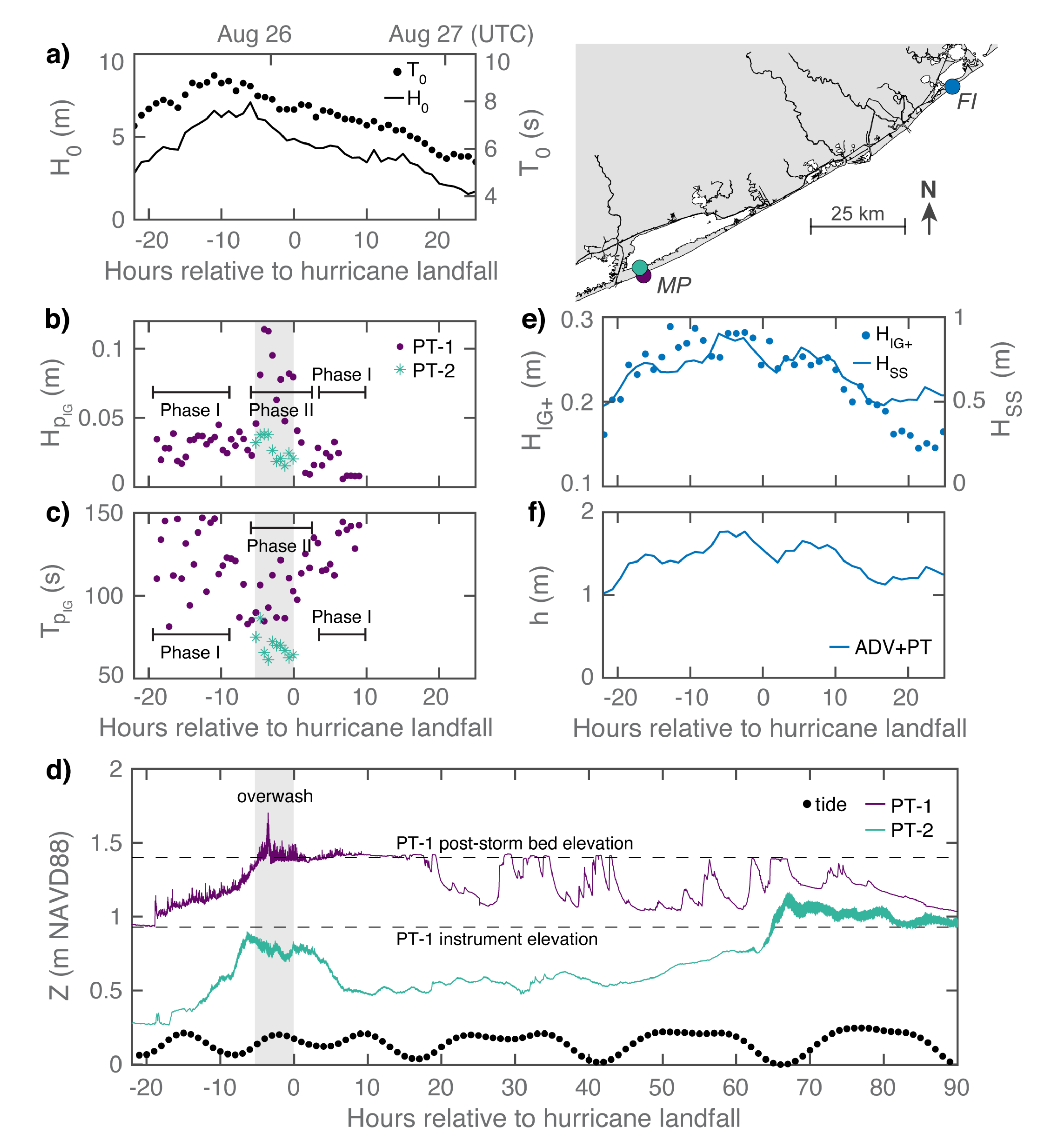
Coastal flooding extended far east of hurricane landfall, reaching 0.6 to 1.2 m above ground level through the upper Texas coast [36]. At the Matagorda Peninsula field site, located ∼200 km northeast of hurricane landfall, coastal flooding commenced at least 19 h before the storm made landfall, evidenced by a sudden increase in pressure head in the backshore at −18.8 h (Figure 2d). As detailed in Section 2.4, we interpret this increase in pressure head to be associated with a series of large swash events which collectively increased the bed at PT-1 by approximately 10 cm. The maximum seaside pressure head was observed at high tide just prior to storm landfall (−3.5 h), measuring 1.7 m NAVD88 in the backshore. This elevation was in excess of the post-storm berm crest elevation (i.e., 1.2 m NAVD88 at 170 m in Figure 1b), suggesting sea-to-bay directed flow. As detailed in Section 4.2, analysis of backshore and back-barrier wave fields indicates a cross-barrier hydraulic connection existed for at least 5 h (−5 to 0 h). Interestingly, back-barrier water levels peaked when the fetch was maximum in the back-barrier bay—that is, when the wind direction was directed westward at −6 h and 67 h, parallel with the longest axis of the bay (Figure 2d).
Post-storm site reconnaissance revealed geomorphic markers of landward directed flow and overwash at Matagorda Peninsula, including side wall erosion and slumping in the mid-barrier, a wrack line of debris extending just beyond the side walls into surrounding vegetation, landward leaning vegetation, and deposition of storm deposits in both the backshore (Figure 3(I–III)) and back barrier. The storm deposits in the backshore measured 47 cm (Figure 3(III)) and resulted in burial of the well casing. In the back barrier, 12 cm accreted proximate to PT-2 but did not bury the well casing (Figure S1). An unmanned aerial vehicle (UAV) was used in combination with a stereo photogrammetric structure-from-motion (SfM) algorithm to generate a digital elevation map (DEM) one week following the storm (see Supplementary Materials for procedure). Immediate post-storm geomorphic impacts were assessed through comparison of the UAV-SfM DEM with LiDAR collected one year prior (September 2016) as part of the United States Army Corps of Engineers (USACE) National Coastal Mapping Program [37]. Comparison of the pre- and post-storm DEMs shows that resolution (temporal and instrument accuracy) is insufficient for quantifying some of the small-scale morphological changes identified after the storm (e.g., 47 cm of accretion in the backshore). However, large changes to the barrier beach can be clearly identified, including the onshore migration of the berm crest and smoothing of the backshore. While not discussed herein, the immediate post-storm DEM also revealed that the morphology of the backshore was heterogeneous with a slight depression located perpendicular to the surge channel. It is hypothesized that this morphology is the result of bay-to-ocean directed flow far after storm landfall (60–80 h, Figure 2d).
Moving 85 km up the coast and farther from storm landfall, the peak pressure head at the Follets Island field site reached 2 m NAVD88 in the surf zone at −3 h (not shown), which is just shy of the average dune elevation (2.5 m NAVD88, Figure 1c). The bed level at the surf zone measurement location was relatively constant, allowing for robust estimation of the mean water depth h, which measured 1.76 m six hours before storm landfall (Figure 2f). Morphological indicators of dune overtopping or breaching were not identified during post-storm reconnaissance. However, scarping of the dune face and smoothing of the foreshore were prominent, suggesting that the primary storm impact regime was dune collision.
The closest offshore wave measurements to the study sites were recorded at National Data Buoy Center (NDBC) Station 42109, located 125 km southwest of Follets Island in 82 m water depth (Figure 1a). This buoy, which was positioned between Follets Island and Hurricane Harvey’s storm track for the duration of the study period, recorded a maximum significant wave height of 7 m six hours prior to landfall with a corresponding mean spectral period of 8.6 s (Figure 2a).
2.4. Groundwater Effects and Bed Level Change at PT-1
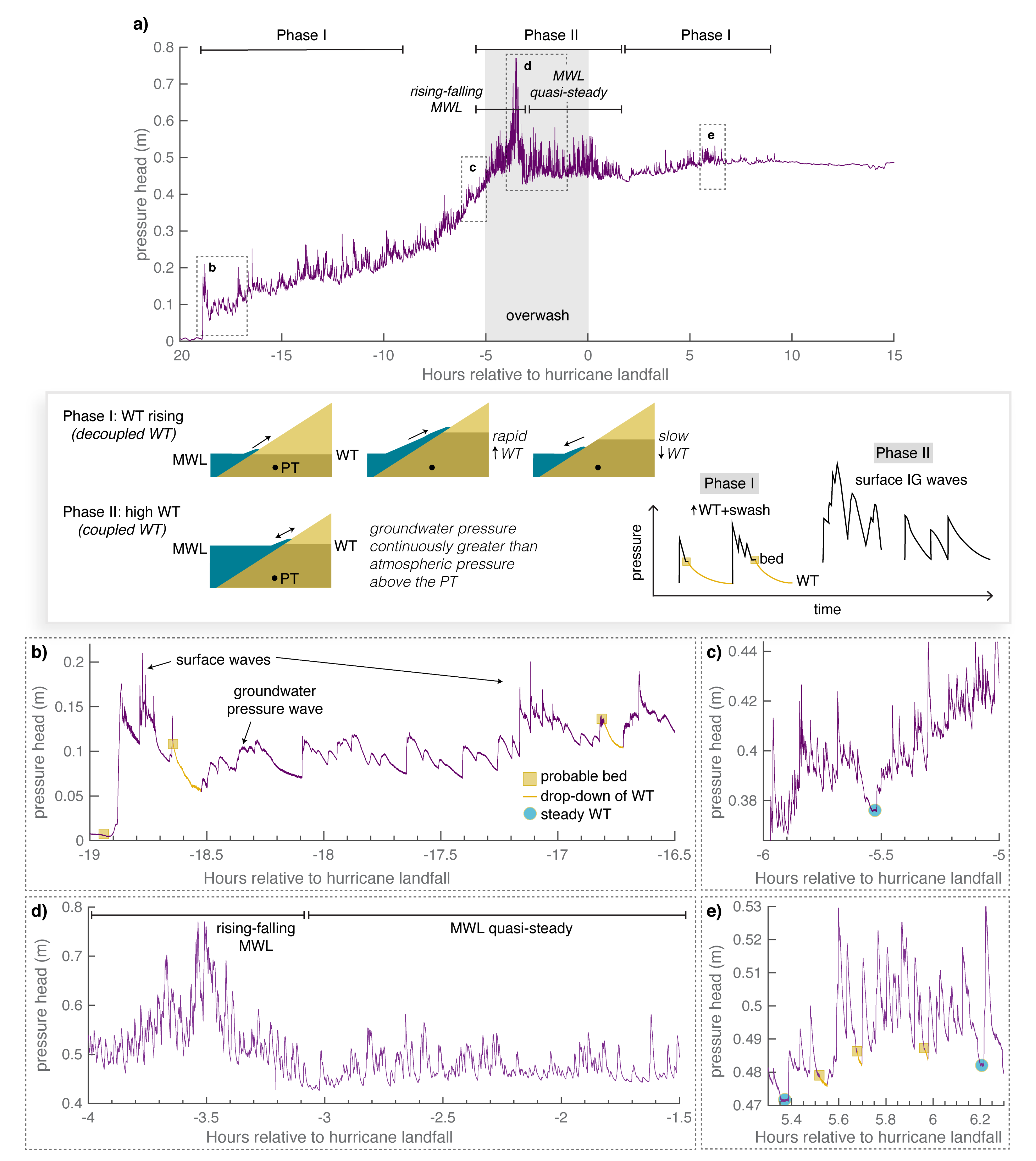
During an accretionary storm event, it would generally be expected that the surf zone mean water level (“MWL”, here the combination of storm tide and wave setup), groundwater table (herein “WT”), and sand bed rise together, albeit at different speeds and with varying time-evolution. Previous studies of groundwater dynamics in the upper swash zone have shown that when the WT becomes decoupled from the sand bed—that is, when the groundwater pressure at the sand bed falls below atmospheric pressure (negative relative pressure)—capillary fringe dynamics and potential pore desaturation modify the groundwater pressure field such that the free surface elevation can not be simply reconstructed using hydrostatic assumptions (e.g., [38,39,40,41,42]). The Phase I schematic in Figure 4 illustrates the effect of the capillary fringe for a single swash event with a decoupled WT (i.e., the WT is located between the PT and the sand bed). With passage of the swash tongue, there is a sharp increase in measured pressure head, which is a summation of the rapid rise of the WT to the elevation of the sand bed and the swash tongue depth. The backwash is then characterized by two pressure decays: a first rapid decay corresponding to the swash tongue retreat until the free surface reaches the sand bed, followed by a slower pressure decay as the WT returns to its baseline elevation [42]. Under favorable conditions of WT and MWL elevations, the change in pressure decay rate may be used to track the sand bed elevation (see Figure 4E in Sous et al. [42]). Overall, this process results in an asymmetric pressure head fluctuation that is lower in frequency than the initial swash or surface wave forcing. By contrast, a coupled WT regime—that is, a regime with a permanently saturated sand bed and positive relative groundwater pressure (even between swash events, Phase II schematic in Figure 4)—allows for direct hydrostatic reconstruction of the free surface elevation from a buried PT. Given that 47 cm of sediment were observed to have accreted in the backshore at Matagorda Peninsula during post-storm reconnaissance, it is important to distinguish during what time periods the measured pressure field at PT-1 can be assumed hydrostatic with a fully coupled sand bed and WT. In the interpretation that follows, we combine both qualitative and statistical analysis of the pressure head time series to identify with high confidence a 7 h period of fully saturated sand bed (−5.5 and 1.5 h) wherein pressure head fluctuations are assumed to be hydrostatic and representative of surface waves. Note that this groundwater analysis and future studies would be improved by external bed-level tracking, control points, and additional instrumentation.
The first overall insight of temporal changes in pressure head in Figure 2d is that PT-1 was devoid of wave-like signatures in the typical sea-swell and IG frequency range after 9 h. Before this time (−18 to 9 h), pressure head increased steadily up to the elevation of instrument burial. Thereafter (9 to 90 h), pressure head slowly returned to pre-storm (atmospheric) levels, punctuated by large (0.4 m), long-period (5–10 h periods) fluctuations. We interpret this time of heightened pressure head between 9 and 20 h as an elevation of the WT after wave and surge-driven flooding with the subsequent WT pulses up to the elevation of the sand bed attributed to astronomical tides and other storm-scale forcing (20 to 90 h).
The time period where pressure head is characterized by wave-like signals in the sea-swell and IG frequency range (−18 to 9 h) can be subdivided into two primary phases (Figure 4a). During Phase I (−18.8 to −9 h and 1.5 to 9 h), the WT, MWL, and bed are rising, but the WT is decoupled from the sand bed and capillary fringe effects are frequently observed and thus significantly influence the pressure head variance. As illustrated in Figure 4b, the first half hour of coastal flooding contains many rapid increases in pressure head, corresponding to passage of sequential swash events. The slow pressure decay observed at −18.6 h (nearly 7 min long) represents the first drop-down of the WT after this series of swash. This WT drop-down is followed by a series of waveforms with smooth faces and crests reaching an elevation of ∼12 cm above the PT (−18.5 to −18.1 h). These waveforms are hypothesized to be groundwater pressure waves that initiate lower in the beachface and travel horizontally through the WT to the sensor location, sometimes extending up to the elevation of the sand bed (i.e., oscillation of the WT). The probable sand bed elevation during Phase I is delineated by tracking sequential instances of pressure waveforms that show step-wise WT decays with clear inflection points after passage of swash (more closely illustrated through the pressure head time series schematic in Figure 4 for Phase I). For example, the first instance of sequential swash events at −18.8 h bring approximately 10 cm of sand, otherwise the pressure signal should have returned (nearly) to the initial pressure head position. While interpretative, this form of bed-level tracking gives an overall picture of morphological evolution during the early phase, and late phase (1.5 to 9 h, discussed below), of coastal flooding. Viewed cumulatively, Phase I is characterized by sequential swash events that result in rapid sand accumulation, followed intermittently by periods where the pressure head signal is representative of groundwater fluctuations due to a progressively rising MWL but lagged WT.
Between −9 and −5.5 h, very few WT drop-downs (and sand bed uncoupling events) are observed. The last clear WT signal is shown in Figure 4c at −5.5 h. Here, the pressure head of the WT remains steady for approximately one minute before arrival of the next wave.
During Phase II (−5.5 to 1.5 h), the bed appears to be continuously saturated with a tightly coupled WT as there is no clear evidence of capillary fringe effects. Bulk statistics for pressure head indicate that the height and period of pressure signals during Phase II differ from other time periods. Specifically, Figure 2b,c shows that pressure head signals in the IG frequency band (the dominant frequency content) are on average larger in height (maximum m) and shorter in period (–120 s) than the pressure head fluctuations contaminated by capillary fringe effects in Phase I (see Section 3 below for details on spectral analysis). Hence, the pressure head fluctuations during Phase II are assumed to be representative of surface waves.
Qualitative evaluation of the pressure head time series within Phase II reveals additional differences. Between −3.1 and 1.5 h (Figure 4d), pressure head is oscillating around a near constant value, which suggests that the MWL was quasi-steady during this time. At 1.5 h, the first WT drop-down is observed to start from an elevation of 45 cm. Thereafter, WT drop-downs are commonly observed between wave events as the WT becomes decoupled from the progressively rising sand bed (Figure 4e). Earlier in Phase II (−5.5 to −3.1 h), pressure head fluctuations rarely oscillate around a constant value as the MWL, and perhaps the bed, is rising and falling.
Lastly, the mean spectral period of the IG pressure head fluctuations throughout Phase II are long (1.5 to 2 min). Given the flat to downward slope of the backshore, we consider the IG pressure head signals during Phase II to be representative of IG waves slowly inundating the backshore and propagating through the surge channel and into the back barrier during overwash.
3. Methods
3.1. Wave Statistics
In the analysis of IG wave dynamics that follows, continuous time series of pressure head were windowed to ∼34 min (Matagorda Peninsula) and ∼68 min (Follets Island) intervals for use in spectral analysis. These window sizes were chosen so to maximize the degrees of freedom (dof) in spectral estimates while maintaining high resolution at IG frequencies and stationarity, which through review of bulk statistics, was found to vary at the two sites. In the surf zone (Follets Island), time series of shoreward () and seaward () propagating waves were constructed using co-located measurements of pressure head and cross-shore velocity u (assuming normal wave incidence) [43].
All power spectra were generated using high resolution multitaper spectral estimation [44], as elaborated upon below. Wave power spectra in the surf zone were corrected for depth attenuation of the pressure signal using linear finite-depth theory. Pressure head power spectra (Matagorda Peninsula, PT-1 only) were corrected for depth attenuation of the pressure signal at sea-swell frequencies using poro-elastic theory [45]. Wave and pressure head statistics were calculated directly from power spectra over the IG (0.003–0.04 Hz) and sea-swell (0.04–0.25 Hz) frequency bands. Prior to calculation of wave statistics, pressure head time series were de-tided and then high-pass filtered to isolate IG wave and sea-swell signals from storm-driven (non-tidal) and tidal residuals. High-pass filtering of the data was accomplished by first twice passing (forward and backward) a low-pass three-pole Butterworth filter with a cutoff frequency of 0.002 Hz and then subtracting the low-pass filtered time series from the original. This methodology ensures that most energy related to storm-driven non-tidal residuals is removed without significantly modifying IG wave oscillations close to the minimum expected IG frequency (0.003 Hz). Where utilized herein, the high-pass filtered records are referred to as “high-frequency” time series.
3.2. Spectral Estimation
Here, we employ the Thomson multitaper method of spectral estimation [44]. In contrast with conventional spectral estimates, the multitaper spectral estimate offers improved bias while also reducing variance due to the use of many optimal data windows [46]. Each time record is windowed separately with members of the Slepian family of tapers and then Fourier transformed to yield raw periodograms called eigenspectra. Due to the orthogonality of the Slepian data windows, eigenspectra are statistically independent. Averaging of the eigenspectra over the bandwidth (here using adaptive weighting) results in multitaper estimates that are correlated over (), with essentially no correlation outside this band. The choice of bandwidth is a trade-off between variance reduction and frequency resolution. In the multitaper algorithm used here [47], K Slepian tapers were computed for a fixed time-bandwidth product (i.e., K = − 1). Choices for the free parameter were selected by evaluating (1) graphically the power spectrum in terms of over- or under-smoothing, and (2) the Thomson F-test, which can be used to locate significant harmonic components in a data record [44]. The final multitaper spectral estimates for each ∼34 min (∼68 min) data window were generated using = 5 (8) and K = 9 (15), yielding a passband bandwidth of 0.0049 Hz (0.0039 Hz) and about 16 (28) dof per frequency. Time series were additionally prewhitened prior to spectral estimation by applying a finite-impulse response filter in the time domain.
3.3. Multitaper Bispectral Estimation
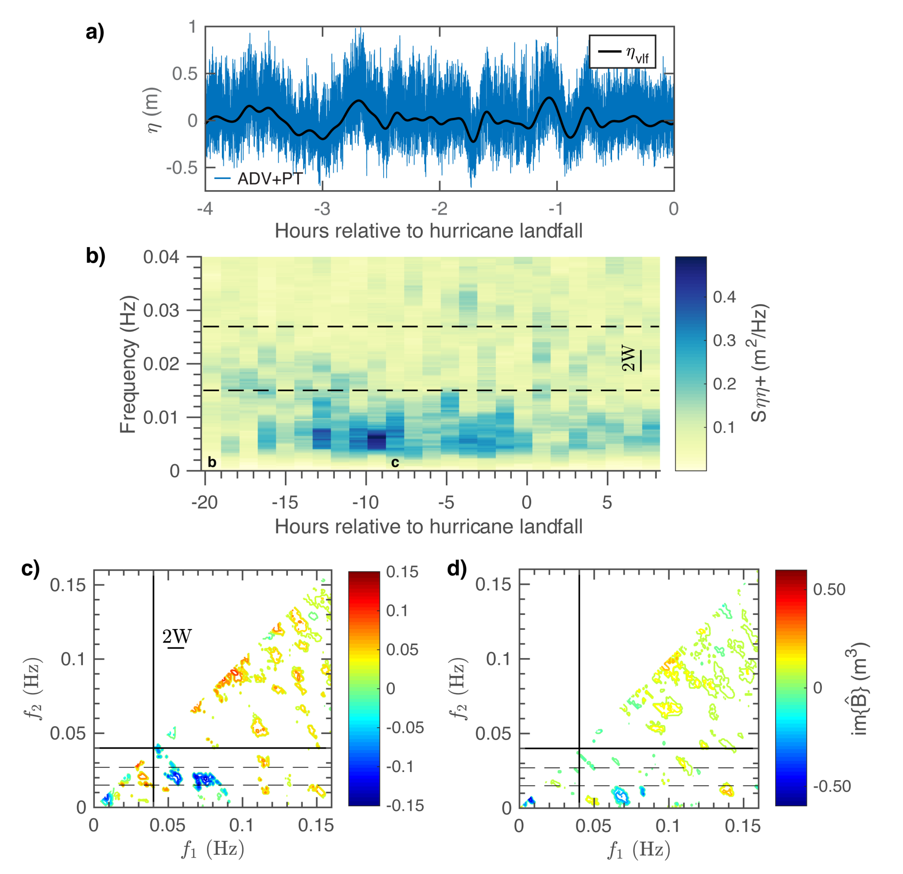
Whereas the power spectrum is a frequency domain decomposition of the power in a signal, the bispectrum is the decomposition of the third moments of a process, which are the skewness (the sum of the real part of the bispectrum) and the asymmetry (the sum of the imaginary part of the bispectrum). The imaginary component of the bispectrum im provides insight on energy exchange within wave triads (, , = + ). Here, we adopt the same representation of im as de Bakker et al. [31] where color is used as a proxy for the magnitude and direction of energy transfers (e.g., Figure 5c,d). Positive (red) values of im indicate a transfer of energy from and to the wave component with sum frequency . Conversely, negative (blue) values represent a transfer of energy from the sum frequency to and , which results in growth of the lower-frequency wave components. Due to the symmetry of the bispectrum, only the triangular region defined by is presented.
While a complete theoretical description of bispectral analysis is beyond the scope of this study (see Collis et al. [48], Elgar and Guza [49], and for multitapers [50]), in practice, ensemble averaging of many biperiodograms is needed to reduce variance and increase the statistical stability of bispectral estimates [51,52]. Therefore, the total length of the time series used for bispectral analysis must allow for sufficient segmentation to achieve statistical stability while maintaining stationarity and the desired frequency resolution. The multitaper bispectral estimator (MBE) involves expectation operations without segmentation as the bispectrum is calculated as the weighted sum of all combinations of many Slepian-tapered biperiodograms (see Appendix A). Thus, when using the MBE, fewer independent realizations are needed for ensemble averaging to ensure statistical stability of the bispectral estimate, albeit with the trade-off of a slight loss in frequency resolution. In comparison to frequency merging techniques, Birkelund and Hanssen [53] found that the MBE produces an estimate with a lower variance for a given bias for processes with a small dynamic range in the bispectral domain (as in this present study), and nearly identical statistical properties for processes with a large dynamic range.
Given these favorable statistical qualities, we develop and employ a new MBE algorithm to generate bispectral estimates using 8 (4) ∼9 min (∼17 min) segments, sub-divided from high-passed ∼68 min (∼34 min) windows of (pressure head) at Follets Island (Matagorda Peninsula). The time bandwidth of the bispectral estimates at Follets Island (Matagorda Peninsula) is 3 (5) with 5 (9) Slepian tapers yielding a of 0.0117 Hz (0.005 Hz) and about 64 (64) dof per frequency. Here, dof = for m segments. The ∼17 min time series at Matagorda Peninsula are additionally zero-padded to resolve narrow-bandwidth peaks in the bispectra during overwash. Note that the adjoining segments selected for bispectral analysis were deemed sufficiently stationary such that ensemble averaging is not suspected to affect the statistical significance of the multitaper bispectral estimates.
The bispectrum is often recast into its normalized magnitude and phase, namely the bicoherence and biphase, which give an indication of the degree of phase coupling and phase relationship (respectively) within the (, , = + ) triad. Nonlinear interactions are associated with non-zero values of bicoherence, and because even a truly Gaussian process will have a non-zero bispectral estimate, confidence levels on zero bicoherence are needed to detect significant nonlinear interactions. Here, we propose that the 95% significance level for zero squared bicoherence using the multitaper technique is approximately for tapers, which can be recast as for (as in this study). The mathematical basis of this formulation is outlined and tested in Appendix A. All bispectral (biphase) estimates are set to zero (NaN) below the 95% significance level for zero bicoherence (the square-root of the proposed formulation), which for the ∼9 min (∼17 min) bispectral estimates shown herein is 0.14 (0.11).
4. Results
4.1. Surf Zone Wave Fields
Over the last several decades, the observational understanding of IG wave dynamics in the surf and swash zones on closed sandy beaches stems primarily from field studies conducted along the east and west coasts of the United States, Western Europe, and New Zealand (see Stockdon et al. [54], Bertin et al. [55], and Billson et al. [56] for detailed references of many published works). To date, no field studies have characterized IG waves in the GOM, likely because they are only energetic during extreme storms. Hence, before detailing observations of IG wave transformation during overwash (Section 4.2), we here provide a brief characterization of IG waves in a closed surf zone-beach-dune system during Hurricane Harvey. Surf zone data was not available at Matagorda Peninsula—the site of island overwash—hence, this section examines wave fields in the surf zone for a similar nearshore geometry farther up the coast at Follets Island.
Bulk wave statistics measured in the surf zone at Follets Island are shown in Figure 2e,f. Surf zone wave fields were comprised of energetic sea-swell (<0.90 m significant wave height for a depth <1.8 m), IG waves (<0.29 m significant wave height, incoming only), and wave phenomena at frequencies below IG waves but above known tidal constituents (0.1–3 mHz, 5.6 min to 2.8 h periods) which we herein term the very low frequency (VLF) band. The period of individual VLF fluctuations in the surf zone ranged from ∼8 to 45 min with (peak-to-trough) wave heights of O(0.40 m) occurring twice during the study interval (−18 to −14 h and −5 to 3 h, Figure 5a). As discussed in Section 5, this VLF variability in sea level is hypothesized to be generated by resonant amplification of long waves initiated by atmospheric disturbances accompanying tropical cyclone rainbands (i.e., meteotsunami). While a complete analysis of how these VLF fluctuations influence surf zone processes is beyond the scope of this study, inspection of the wave envelope of the IG wave signal (calculated via the Hilbert transform for bandpass filtered time series, ) during both time periods of large VLF variability revealed that amplitude modulation of IG waves at VLF was relatively small at this surf zone location (<3 cm).
IG waves were only energetic in the surf zone for 42 h proximate to hurricane landfall (significant wave height >16 cm, −22 to 20 h, Figure 2e). For most of this time (−20 to 8 h), alongshore currents were relatively small (<0.3 m/s), the ratio of significant alongshore to cross-shore IG velocities () was less than 0.36, and shear wave contributions to velocity variance over the IG frequency band (calculated following Lippmann et al. [57]) did not exceed 24%. These statistics are similar to those used for quality control of IG wave observations during energetic conditions by e.g., Fiedler et al. [14], and therefore we likewise assume that IG wave observations are not contaminated by vortical motions and that their propagation can be approximated as shore-normal during this time (−20 to 8 h).
On closed beaches, freely propagating IG waves can reflect from the shoreline to form cross-shore standing waves (e.g., [16,58,59,60,61]). Here, we use the shoreward propagating wave component () to generate wave power spectra (Figure 5b) and bispectra (Figure 5c,d) in order to avoid mixing information about shoreward and seaward propagating IG waves. The spectrogram of IG wave power spectra in Figure 5b shows that IG energy was concentrated at middle frequencies (0.015–0.027 Hz) early in the storm (−20 to −17 h) and at low frequencies (0.003–0.015 Hz) proximate to landfall (−17 to 8 h). Bispectral analysis shows negative interactions involving IG waves and the sea-swell spectral peak during both time periods (e.g., im at −19 h in Figure 5c and im at −8 h in Figure 5d). The integrated IG/sea-swell biphase (i.e., the biphase integrated between = 0.04 Hz and the Nyquist frequency, and = 0 to 0.04 Hz) was 111° early in the storm (Figure 5c) and decreased to about −90° proximate to landfall (Figure 5d). This range of IG/sea-swell biphase values is consistent with the values found by Bakker et al. [31] when analyzing the cross-shore evolution of originally (fully) bound IG waves across the surf zone. It is this large phase lag (111°) that enables strong energy transfer to IG waves early in the storm [24,31,62,63,64,65], which, in conjunction with the near-resonance of the quadratic difference interactions [49,66,67], facilitates growth of IG waves in the surf zone. Hence, we hypothesize that IG waves are generated at this mild-sloping field site via the bound wave mechanism [68,69,70]. Consequently, the differences in frequency of the bound IG wave over the course of the storm are likely attributable to changes in the short-wave group period. Lastly, linear regression analysis indicates a positive correlation between and offshore (deep water) wave height (Figure 2a, coefficient of determination of = 0.85 for the total IG frequency band and = 0.76 for the lowest frequency IG waves), a finding consistent with many previous field studies (e.g., [10,15,59]).
4.2. IG Wave Transformation during Overwash
At Matagorda Peninsula, IG waves dominated the backshore (sea-side) wave field for the duration of Phase II—that is, the time period wherein the bed was deemed fully saturated from −5.5 to 1.5 h (Figure 4a) and groundwater pressure head fluctuations can therefore be assumed hydrostatic and representative of surface waves. IG energy was only observed in the back barrier (bay-side) for the five hours prior to hurricane landfall (−5 to 0 h). During this time, the pressure head in the backshore exceeded the measured post-storm berm crest elevation by 0.15 to 0.5 m. Collectively, these observations suggest that this period was characterized by sea-to-bay directed flow (i.e., storm overwash). Notably, sea-swell energy was nil (<0.03 m) at both PT locations on Matagorda Peninsula during overwash.
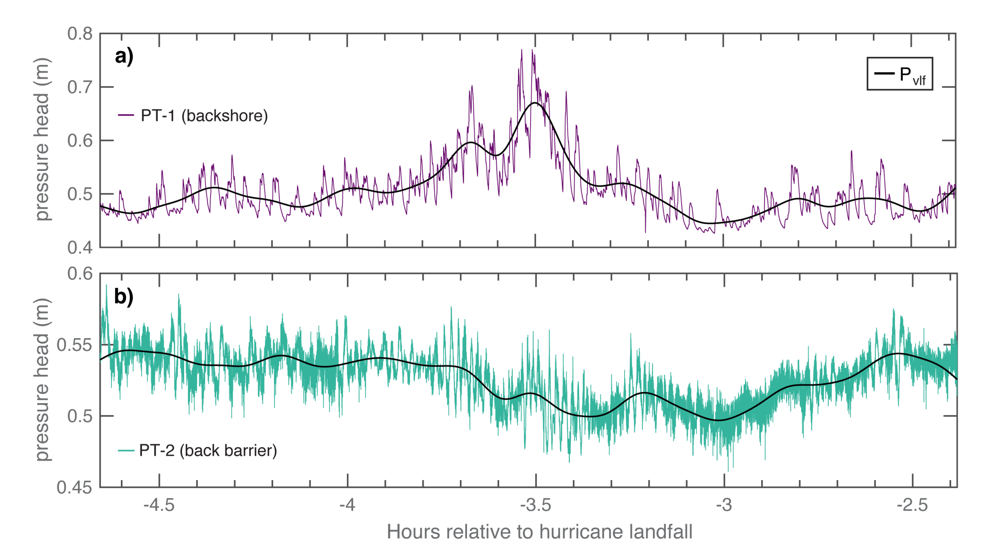
The temporal and spatial evolution of IG waveforms at Matagorda Peninsula is shown in Figure 6 for ∼2 h records of pressure head in the backshore (a) and back barrier (b) during overwash. The largest IG waves in the backshore (maximum peak-to-trough wave height of 22 cm) and back barrier (maximum peak-to-trough wave height of 9 cm) were observed superimposed on the crests of VLF fluctuations in pressure head between −3.8 and −3.3 h. Additionally, the wave envelope of IG waves in the back barrier during this same time period indicates grouping of IG waves at VLF, with small (1 cm), but relatively significant amplitude modulation given the small IG wave heights. Although the bed level and water depth are uncertain in the backshore during this time period (Section 2.4), these observations suggest that the water depth in which IG waves propagated during overwash was episodically modulated by VLF fluctuations in water level (here, ∼17–45 min periods).
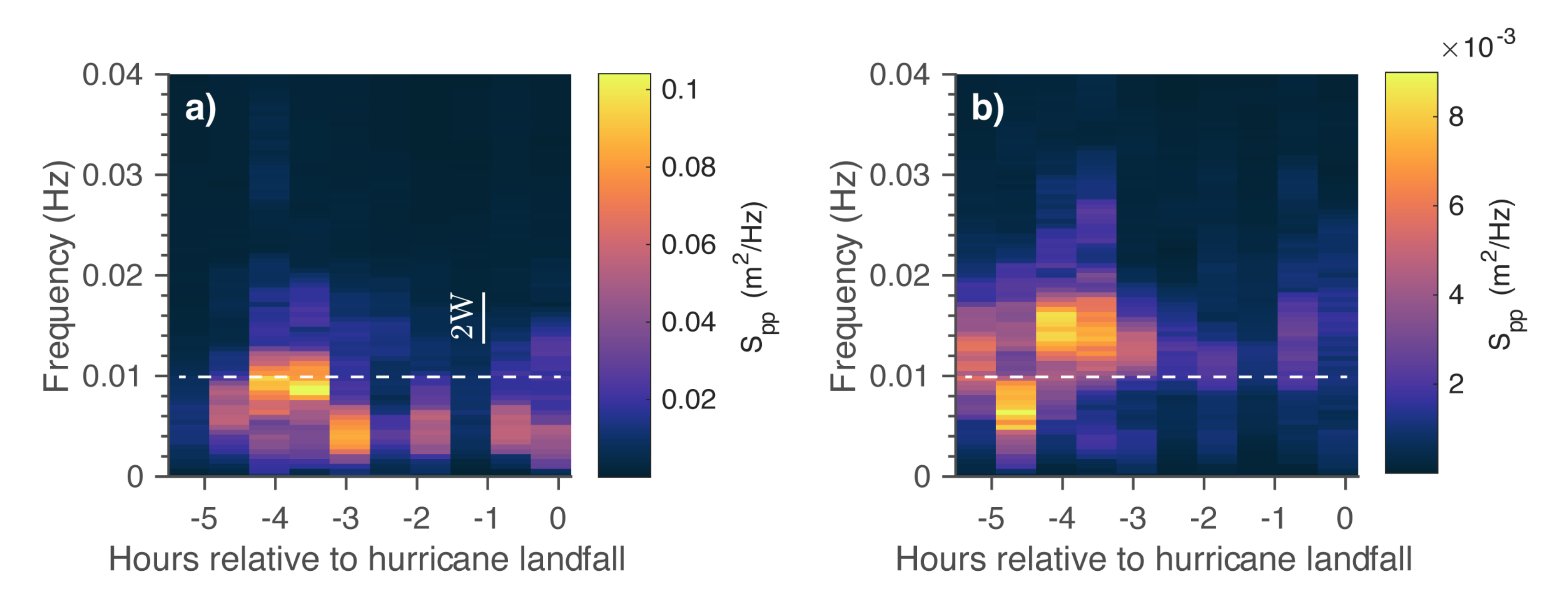
Comparison of IG waveforms in Figure 6a,b qualitatively shows that the measured amplitude, and in some cases the dominant frequency content, of IG waves differed on either side of the barrier island during overwash (see also Figure 2b,c for pressure head statistics). These observations are supported quantitatively in Figure 7 through comparison of IG pressure head power spectra , generated using the high-frequency pressure head ( Hz). Specifically, IG wave energy is concentrated below ∼0.01 Hz in the backshore (Figure 7a) and above this frequency threshold in the back barrier (Figure 7b) for the duration of overwash. In the discussion that follows, we investigate possible mechanisms that could contribute to changes in IG energy and frequency content across the barrier island during overwash.
5. Discussion
The observations presented above confirm that IG waves are an important component of the nearshore wave field during relatively low surge events along this mild-sloping sandy coastline. The relative dominance of IG waves (over gravity waves) during overwash is consistent with previous field studies that have measured wave fields during storm-driven overwash and inundation elsewhere [6,7], and the general assumption of morphodynamic models used to simulate hurricane impact (e.g., [20]). The discussion below investigates how changing water depths, nonlinear energy transfer, and energy dissipation through wave breaking and frictional damping may serve as driving mechanisms for cross-barrier changes in IG energy and frequency content during overwash at Matagorda Peninsula. We conclude with remarks on the potential origin and relative importance of episodic, VLF water-level anomalies on IG wave dynamics and storm processes at both field sites.
5.1. Cross-Barrier Changes in IG Energy during Overwash
As energy can go up and down conservatively as waves propagate over different water depths, it is important to assess to what degree cross-barrier decreases in IG wave amplitude and apparent changes in frequency content are due to changing water depths on either side of the barrier island versus losses from dissipation or nonlinear energy transfer. At Matagorda Peninsula, robust calculation of energy fluxes would require (1) co-located pressure and velocity data to allow for the calculation of incoming and reflected wave components, and (2) more accurate knowledge on water depths (i.e., the frequency-domain separation method of Sherement et al. [61]). Prior to overwash, the last WT signal was observed at 38 cm in the backshore (−5.5 h, Figure 4c). Using this as a lower bound for the potential bed elevation during overwash, the instantaneous water depth, which was modulated by VLF fluctuations, likely never exceeded 30 cm at PT-1 (i.e., at −3.5 h in Figure 6) and was much lower between −3 and 0 h when the MWL was quasi-steady (Figure 4d). Estimation of energy fluxes from surface wave time series in such shallow water (<10 cm) is not straightforward as linear wave theory is unlikely to hold. Instead, as a first-order estimate, we calculate energy flux for the time period between −4 and −3 h when the water depth is expected to be largest. Recognizing that the pressure head is a superposition of incident and reflected waves, but unable to decompose pressure into incoming and outgoing components, we assume unidirectional waves and normal wave incidence at both instrument locations (i.e., all IG wave energy is directed landward) and calculate the bulk IG energy flux F as
where is the long-wave speed and is the energy density calculated using only the autospectra of the pressure head (as opposed to both the autospectra and co-spectrum of pressure head and u [61]). Wave reflection is unlikely to be important given that the morphology of the barrier-island cut is downward sloping between the sensors. While the effect of non-normal wave incidence may be important, as well as other 2D effects such as wave focusing and de-focusing, these assumptions enable an initial estimation (and upper bound) of the cross-barrier change in IG energy flux during overwash, which is represented here through a percent decrease between the backshore and back-barrier sensors: .
The cross-barrier change in IG energy flux is calculated for a minimum and maximum water depth scenario, both of which are summarized in Table 1. Estimates of are obtained from ∼34 min windows of the high-frequency pressure head ( Hz) so to avoid spectral leakage from VLF energy, but the effect of the VLF fluctuations on changing water levels is encompassed within the range of mean water depths for both scenarios. For the range of water depths explored here, we find that IG energy flux decreases between 79 and 86% across the barrier-island cut. Partitioning of into low and high-frequency components (above and below 0.01 Hz, respectively), this decrease in IG energy flux is found to be larger for the lowest-frequency IG waves (92–96%).
Cross-barrier decreases in IG energy flux could be the result of IG energy dissipation due to wave breaking or frictional damping (as in Engelstad et al. [6]), as well as nonlinear energy transfer. Here, we explore how nonlinear triad interactions influence the spectral evolution of IG waves in the backshore during island overwash. While use of the total wave signal, as opposed to only the incoming wave signal, can reduce bicoherence levels due to the presence of reflected waves [49], de Bakker et al. [31] found that, for IG–IG interactions in the inner surf zone, the bispectral signal was not considerably altered by these reductions in bicoherence. Here, we assume that the bispectral signals of IG–IG interactions in the shallow waters of the backshore are likewise robust to reductions in bicoherence due to reflected IG waves, which are assumed to be negligible due to the flat to downward-sloping morphology of the backshore. Note that bispectral analysis is not performed on time records from the back barrier due to very low energy levels which could inflate bicoherence estimates.
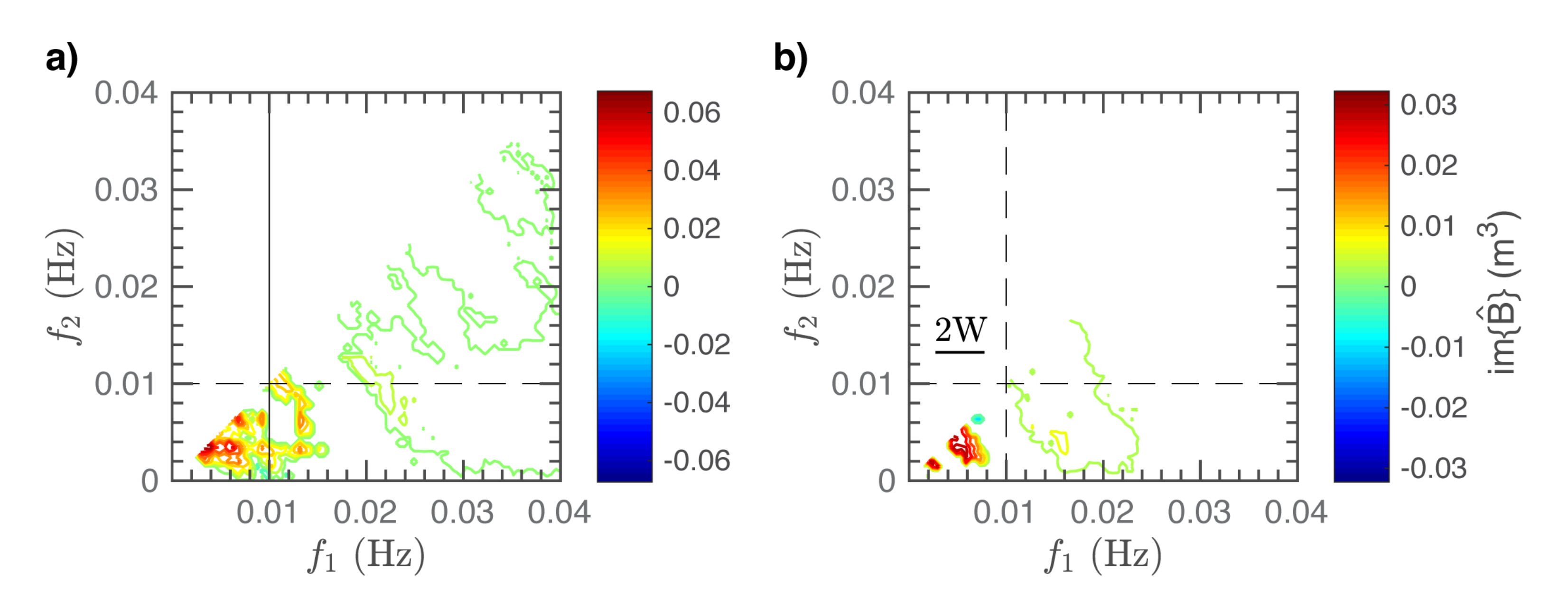
Figure 8 shows two bispectral estimates during overwash (a: −4 to −3 h, b: −3 to −2 h), each generated using four 17 min segments of the high-frequency pressure head, sub-divided from two sequential ∼34 min records in the backshore. While the water level and IG wave amplitudes are non-stationary during these time periods (Figure 7a), the peak IG wave frequency was deemed sufficiently stationary such that ensemble averaging of individual bispectra is not expected to affect the frequency content of the final bispectral estimate. As evidenced by the positive interactions below 0.01 Hz in Figure 8a,b, nonlinear triad interactions result in a transfer of energy from the dominant IG spectral peak ( Hz) to higher harmonics ( Hz). Such nonlinear energy transfers to bound (phase-locked) harmonics are known to play a large role in the spectral evolution of both breaking [33] and non-breaking waves [27] in shallow water. While we cannot discern whether the lowest-frequency IG waves are breaking, the biphase integrated over the IG frequency band was −24° for Figure 8a and −53° Figure 8b. As shown by Masuda and Kuo [71] for harmonic interactions, the biphase can be used to infer nonlinear modifications to the wave shape, and the biphase of IG waves observed here are characteristic of asymmetric waveforms that are not fully sawtooth in shape (−90° as in Bakker et al. [31]). Regardless, if this pattern of nonlinear energy transfer persists into the back barrier during overwash—that is, if the bound harmonics continue to grow across the wide barrier-island cut—the IG wave shape will become more nonlinear, and eventually may steepen and break. This hypothesis is additionally supported by the observations of Engelstad et al. [6] which suggest that small water depths enhance the steepening of IG waves during island inundation, which consequently leads to energy dissipation due to wave breaking. While wave breaking was suggested by Engelstad et al. [6] to dominate over dissipation by bottom friction during shallow inundation events, at Matagorda Peninsula, we cannot isolate the main dissipation mechanisms nor quantify their contribution to cross-barrier changes in IG energy. However, given the nonlinear triad interactions in Figure 8, it is likely that the frequency-dependence of IG energy loss across the barrier island is in part owing to nonlinear energy transfer from the low-frequency IG peak to higher IG frequencies (above 0.01 Hz).
5.2. Importance and Origin of VLF Variability
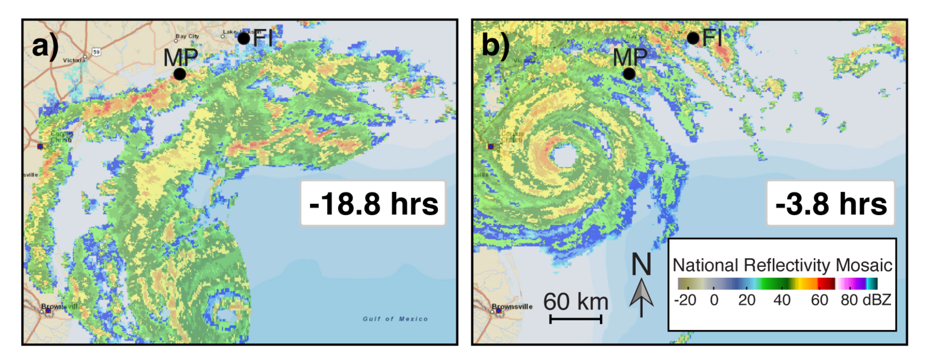
VLF variability in water level (0.1–3 mHz, 5.6 min to 2.8 h periods) was observed at all instrument locations episodically throughout the storm (Figure 5a, Figure 7). The typical periods of the individual VLF fluctuations ranged from 17 to 45 min at all but the surf zone location, where the individual periods spanned a larger range (∼8 to 45 min). Although wave phenomena have been observed with periods upwards of ∼10 min in the nearshore on beaches elsewhere (i.e., shear waves (e.g., [72]), forcing from wave groups [73]), the VLF fluctuations observed during Hurricane Harvey were typically much lower in frequency and spanned a larger range of frequencies. Recently, it was shown by Shi et al. [74] and Olabarrieta et al. [75] that atmospheric disturbances accompanying tropical cyclone rainbands (TCRs) can trigger meteotsunami in the GOM. The Next Generation Weather Radar (NEXRAD) reflectivity mosaics from the National Oceanic and Atmospheric Administration (NOAA) in Figure 9 show that land-falling TCRs were positioned just offshore Matagorda Peninsula coincident with the abrupt increase in pressure head, and initiation of coastal flooding, in the backshore at −18.8 h (Figure 4b), as well as immediately prior to the peak water level when the largest IG waves were superimposed on VLF fluctuations in pressure head (Figure 6). Hence, we hypothesize that the VLF fluctuations in pressure head at Matagorda Peninsula during overwash are likewise meteotsunami triggered by TCRs. Furthermore, previous studies have shown that low-frequency modulation of water depth by IG waves can increase the number of bore-bore capture events [76], and thereby lead to generation of large wave runup [77]. This phenomenon could explain the sudden onset of flooding by sequential swash events at −18.8 h that resulted in rapid sand accumulation (10 cm) in the backshore if the water depth was indeed modulated by a VLF fluctuation, a hypothesis that cannot be explored here. Regardless, the VLF fluctuations observed during Hurricane Harvey are an unexpected contribution to the incident wave field that influenced storm processes in the very nearshore.
6. Conclusions
Observations of wave fields at two neighboring barrier islands during Hurricane Harvey add valuable field documentation to the paucity of knowledge related to the role and duration of wave processes during hurricane impact. We show that IG waves are an important component of the nearshore wave field in the Gulf of Mexico during hurricanes. At one location, IG waves overtopped the berm crest and propagated onshore through a pre-existing and low-lying barrier-island cut during sea-to-bay directed flow (i.e., overwash) for a period of 5 h. IG waves dominated the incident wave field (over gravity waves) during overwash, and were episodically superimposed on very low frequency storm-driven variability in water level (0.1–3 mHz, 5.6 min to 2.8 h periods). Very-low frequency sea-level anomalies were also observed episodically at a closed beach farther up the coast and are hypothesized to be meteotsunami triggered by atmospheric disturbances during passage of tropical cyclone rainbands across the wide continental shelf. The slow variation of total water depth associated with this phenomenon is found to slightly modulate IG wave heights in very shallow water. This nonlinear process warrants further study, as does the contribution of these very low frequency sea-level anomalies to coastal flooding and morphological change.
The energy content of IG waves was largely modified across the barrier-island cut during overwash. Our data show that, for a range of probable water depths during overwash (given uncertainty in bed-levels), IG energy loss across the barrier-island cut was frequency dependent and greatest for the lowest-frequency IG waves, below ∼0.01 Hz (92–96% decrease in IG energy flux). Bispectral analysis of IG waves on the sea-side of the barrier island during overwash show that nonlinear triad interactions result in a transfer of energy from the dominant IG spectral peak ( Hz) to higher harmonics within the IG frequency band ( Hz). These triad interactions may contribute to IG wave steepening and eventual dissipation of IG wave energy through wave breaking, a hypothesis that necessitates detailed numerical modeling of dissipation mechanisms (including frictional damping). Independent of wave breaking, if nonlinear energy transfers from the low-frequency IG peak to its harmonics ( Hz) persist through the barrier-island cut into the back barrier, it is likely that these nonlinear triad interactions contribute to the frequency-dependence of cross-barrier IG energy loss during this storm. These observations highlight the complex transformation of the incident wave field across long expanses of shallow water depths on mild, sandy slopes and underscores incorporation of nonlinear energy transfer when detailing energy balances during overwash and inundation.
Supplementary Materials
The following are available online at https://www.mdpi.com/2077-1312/8/8/545/s1, Figure S1: PT Schematics, Figure S2: DEM Workflow.
Author Contributions
K.A. and J.F. collected the field data; K.A. performed the data analysis; K.A. and M.T. wrote the manuscript and developed the methodology; D.S. guided interpretation of the field data and edited the manuscript; J.F. acquired funding, conceptualized the project, and edited the manuscript. All authors have read and agreed to the published version of the manuscript.
Funding
Funding was provided by the National Science Foundation (NSF) under Grant No. OCE-1760713, an Institutional Grant (NA14OAR4170102) to the Texas Sea Grant College Program from the National Sea Grant Office, National Oceanic and Atmospheric Administration. J.F. received additional support under NSF Grant No. OISE-1545837. Further support was provided by Texas A&M University at Galveston and the SSPEED Center at Rice University. K.A. was additionally supported by the Link Ocean Engineering and Instrumentation Ph.D. Fellowship Program during this project.
Acknowledgments
We thank all members of the COASTRR team for their help with deployment and recovery of field instrumentation in harsh conditions. We would like to acknowledge the support of Casey Dietrich, Clint Dawson, and the Texas Advanced Computing Center for use of their computing resources. In addition, we greatly appreciate feedback received from Dave Thomson, Steve Elgar, Britt Raubenheimer, and two anonymous reviewers which improved the quality of this work. The offshore wave observations (https://www.ndbc.noaa.gov), radar reflectivity mosaics (https://gis.ncdc.noaa.gov/maps/ncei/radar), and water level observations and predictions (https://tidesandcurrents.noaa.gov) used in this study are all publicly available. All other data is available through the DesignSafe-CI Data Depot: https://doi.org/10.17603/ds2-m0bc-n829.
Conflicts of Interest
The authors declare no conflict of interest. All views, opinions, findings, conclusions, and recommendations expressed in this material are those of the authors and do not necessarily reflect the opinions of the funding agencies.
Appendix A. Zero-Level Bicoherence for the Multitaper Method
Recalling that (1) a discretely sampled Gaussian process with truly independent modes will have a non-zero bispectrum due to its finite length, and (2) nonlinear interactions are associated with non-zero values of bicoherence, it is clear that confidence limits on zero bicoherence are needed to distinguish significant nonlinear interactions. Haubrich [51] suggested that the estimated squared bicoherence for a Gaussian process, which has a true , using the segment-averaged biperiodogram and periodogram will approach a chi-square distribution with parameter in the limit of large degrees of freedom (dof). The positive bias of this estimator can be approximated as [78]
which for Gaussian data and m segments reduces to
where dof [51]. From the properties of a distribution, it can then be shown that the 95% significance level on zero squared bicoherence using this technique is approximately 6/dof.
It was later demonstrated numerically by Elgar and Guza [79] that the distribution of for a Gaussian process is not sensitive to smoothing operations, namely via ensemble averaging and frequency merging, and remains distributed even at low dof. The multitaper bispectral estimator (MBE) acts as an ideal normalized hexagonal smoothing window in the bi-frequency domain [80]. Thus, given that the multitaper eigencoefficients are likewise individually distributed as complex Gaussian [44], we expect the squared bicoherence using the segment-averaged MBE to be asymptotically distributed for . To aid in discussion, this hypothesis will initially be accepted and the goodness of fit of a distribution will be addressed thereafter.
The estimated squared bicoherence using the multitaper technique is defined here as
where and are the estimated second and third moments and are related to the multitaper power spectral and bispectral estimates by
and
where N is the length of the data record [80]. While this definition of squared bicoherence differs from Haubrich [51] and others [48,52,79], in these studies, the bispectrum is defined as the segment-averaged third moment , where is the Fourier transform of n discrete observations, and is not equivalent to the process bispectral estimate from the MBE (see Equations (7)–(9) in Thomson [81]). As in Kim and Powers [52], we neglect the statistical variability of the denominator in Equation (A3)—that is, we use the true value of instead of the estimated value—and thus the expectation of the multitaper squared bicoherence can be recast in terms of the process bispectrum as
Using Birkelund et al. [50]’s approximation for the variance of the MBE for Gaussian data,
it follows that for m segments
Thereby, in the limit of large dof for distributed , we propose that the 95% significance level for zero squared bicoherence is approximately . As elaborated below, this formulation only holds for but provides a reasonable estimate for when recast as .
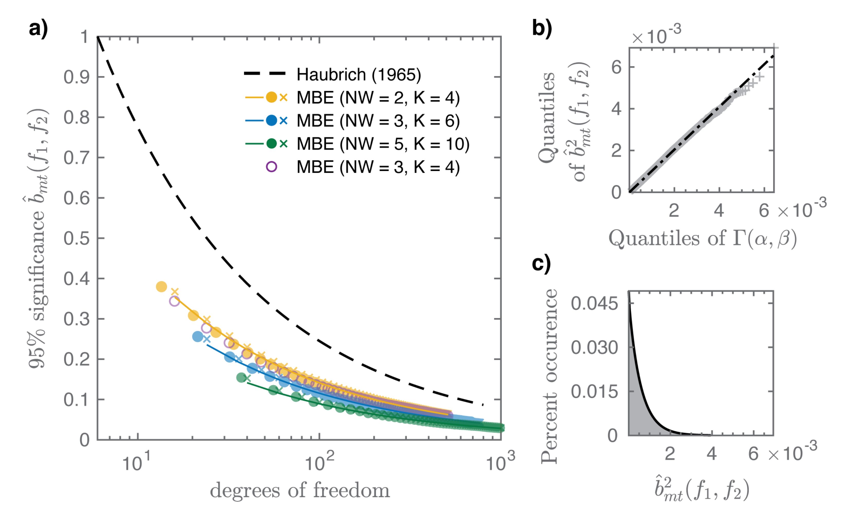
Following the methodology of Elgar and Guza [79], we test this proposed formulation for a synthetic time series of 32,768 values from a zero mean unit variance Gaussian process, divided into 64 records containing 512 data points each. The 95% significance levels for zero bicoherence (the square-root of the proposed formulation) are plotted against dof in Figure A1a for both adaptive (circle) and non-adaptive (x) multitaper bicoherence estimates. The adaptive multitaper estimate is generated using a weighted average of the Slepian-tapered biperiodograms, whereas the non-adaptive estimate incorporates all K tapers. Theoretical values for three typical time-bandwidth products ( 2, 3, 5) and corresponding tapers are represented by solid lines. Additionally, data are shown for a single case of (, ). The theoretical 95% significance level given by Haubrich [51] is also included for comparison of the multitaper technique to traditional ensemble averaging.
Figure A1.
(a) the 95% significance level for zero bicoherence as a function of degrees of freedom for the adaptive (circle) and non-adaptive (x) multitaper bispectral estimator (MBE). Theoretical significance levels are represented by solid lines for time-bandwidth products = 2, 3, 5 with tapers, as is the 95% confidence bound (dashed) for the traditional segment-averaged technique detailed by Haubrich [51]; (b) quantile–quantile plot of using the adaptive MBE for () versus a theoretical gamma distribution (equivalently a scaled distribution) and (c) the maximum-likelihood estimate fit of a gamma distribution (parameters in Table A1).

As shown in Figure A1a, the proposed theoretical formulation matches the calculated values of zero-level bicoherence well, even at low dof (e.g., dof = 32) for MBE estimators where (yellow, blue). Differences between the 95% confidence bounds for the non-adaptive (x) and adaptive (circle) multitaper bicoherence estimates are negligible. Significance levels decrease only slightly as the bandwidth over which the estimate is smoothed increases and hence variance reduction between MBE estimators is primarily a function of the number of tapers. As shown for the case where and , the theoretical approximation using tapers but a smaller time-bandwidth product of is still a reasonable and conservative estimate for zero level bicoherence. Therefore, we suggest use of the theoretical confidence limit in the form for .
The low values of zero-level bicoherence achieved by the MBE are attained through less segmentation of the data record than traditional ensemble averaging (i.e., Haubrich [51]), albeit at the trade-off of a reduction in frequency resolution. When compared to frequency smoothed bispectral estimates (which likewise increase the dof with the trade-off of reduced frequency resolution), the MBE produces nearly identical statistical properties for processes with a large dynamic range, and lower variance for a given bias for processes with a small dynamic range [53].
Throughout the preceding analysis, the assumption was made that is distributed. The validity of this assertion is tested here by evaluating the goodness of fit of the distribution with a two parameter gamma distribution characterized by shape parameter and scale parameter (the distribution mean). The distribution is a particular form of the distribution with and . Here, the distribution of is transformed by which acts to squeeze the probability density function (PDF). The goodness of fit of to this theoretical distribution is shown in Figure A1b for () through a quantile–quantile plot. The relationship is nearly linear, with some deviation in the extremities, indicating good agreement between a scaled distribution and the data. The parameters of the maximum-likelihood estimate fit of a distribution to are in good agreement with theory (Table A1), which is shown for () in Figure A1c, although the actual PDF has a longer tail.

Table A1.
Gamma distribution parameters (, ) for theoretical and maximum-likelihood estimates (MLE) of with confidence limits (CL) for two example time-bandwidth products .
Table A1.
Gamma distribution parameters (, ) for theoretical and maximum-likelihood estimates (MLE) of with confidence limits (CL) for two example time-bandwidth products .
| [95% CL] | [95% CL] | |||
|---|---|---|---|---|
| 2 | 1 | 0.00130 | 0.99 [0.98 1.01] | 0.00135 [0.00133 0.00137] |
| 3 | 1 | 0.00058 | 0.99 [0.97 1.00] | 0.00060 [0.00058 0.00061] |
References
- Sallenger, A.H., Jr. Storm impact scale for barrier islands. J. Coast. Res. 2000, 16, 890–895. [Google Scholar]
- Holland, K.T.; Holman, R.A.; Sallenger, A.H. Estimation of overwash bore velocities using video techniques. In Coastal Sediments; American Society of Civil Engineers: Reston, VA, USA, 1991; pp. 489–497. [Google Scholar]
- Hoekstra, P.; Haaf, M.T.; Buijs, P.; Oost, A.; Breteler, R.K.; van der Giessen, K.; van der Vegt, M. Washover development on mixed-energy, mesotidal barrier island systems. In Proceedings of the Coastal Dynamics 2009: Impacts of Human Activities on Dynamic Coastal Processes; World Scientific: Singapore, 2009; pp. 1–12. [Google Scholar] [CrossRef]
- Matias, A.; Ferreira, Ó.; Vila-Concejo, A.; Morris, B.; Dias, J.A. Short-term morphodynamics of non-storm overwash. Mar. Geol. 2010, 274, 69–84. [Google Scholar] [CrossRef]
- Sherwood, C.R.; Long, J.W.; Dickhudt, P.J.; Dalyander, P.S.; Thompson, D.M.; Plant, N.G. Inundation of a barrier island (Chandeleur Islands, Louisiana, USA) during a hurricane: Observed water-level gradients and modeled seaward sand transport. J. Geophys. Res. Earth Surf. 2014, 119, 1498–1515. [Google Scholar] [CrossRef] [Green Version]
- Engelstad, A.; Ruessink, B.; Wesselman, D.; Hoekstra, P.; Oost, A.; van der Vegt, M. Observations of waves and currents during barrier island inundation. J. Geophys. Res. Ocean. 2017, 122, 3152–3169. [Google Scholar] [CrossRef] [Green Version]
- Lashley, C.H.; Bertin, X.; Roelvink, D.; Arnaud, G. Contribution of Infragravity Waves to Run-up and Overwash in the Pertuis Breton Embayment (France). J. Mar. Sci. Eng. 2019, 7, 205. [Google Scholar] [CrossRef] [Green Version]
- Huntley, D.; Guza, R.; Bowen, A. A universal form for shoreline run-up spectra? J. Geophys. Res. 1977, 82, 2577–2581. [Google Scholar] [CrossRef]
- Guza, R.; Thornton, E.B. Swash oscillations on a natural beach. J. Geophys. Res. Ocean. 1982, 87, 483–491. [Google Scholar] [CrossRef]
- Ruggiero, P.; Holman, R.A.; Beach, R. Wave run-up on a high-energy dissipative beach. J. Geophys. Res. Ocean. 2004, 109. [Google Scholar] [CrossRef] [Green Version]
- Senechal, N.; Coco, G.; Bryan, K.R.; Holman, R.A. Wave runup during extreme storm conditions. J. Geophys. Res. Ocean. 2011, 116. [Google Scholar] [CrossRef] [Green Version]
- Hughes, M.G.; Aagaard, T.; Baldock, T.E.; Power, H.E. Spectral signatures for swash on reflective, intermediate and dissipative beaches. Mar. Geol. 2014, 355, 88–97. [Google Scholar] [CrossRef] [Green Version]
- Ruessink, B. Observations of turbulence within a natural surf zone. J. Phys. Oceanogr. 2010, 40, 2696–2712. [Google Scholar] [CrossRef] [Green Version]
- Fiedler, J.W.; Brodie, K.L.; McNinch, J.E.; Guza, R.T. Observations of runup and energy flux on a low-slope beach with high-energy, long-period ocean swell. Geophys. Res. Lett. 2015, 42, 9933–9941. [Google Scholar] [CrossRef] [Green Version]
- Inch, K.; Davidson, M.; Masselink, G.; Russell, P. Observations of nearshore infragravity wave dynamics under high energy swell and wind-wave conditions. Cont. Shelf Res. 2017, 138, 19–31. [Google Scholar] [CrossRef]
- Bertin, X.; Martins, K.; de Bakker, A.; Chataigner, T.; Guérin, T.; Coulombier, T.; de Viron, O. Energy transfers and reflection of infragravity waves at a dissipative beach under storm waves. J. Geophys. Res. Ocean. 2020, 125, e2019JC015714. [Google Scholar] [CrossRef]
- Bertin, X.; Olabarrieta, M. Relevance of infragravity waves in a wave-dominated inlet. J. Geophys. Res. Ocean. 2016, 121, 5418–5435. [Google Scholar] [CrossRef] [Green Version]
- Bertin, X.; Mendes, D.; Martins, K.; Fortunato, A.B.; Lavaud, L. The closure of a shallow tidal inlet promoted by infragravity waves. Geophys. Res. Lett. 2019, 46, 6804–6810. [Google Scholar] [CrossRef]
- Mendes, D.; Fortunato, A.B.; Bertin, X.; Martins, K.; Lavaud, L.; Silva, A.N.; Pires-Silva, A.A.; Coulombier, T.; Pinto, J.P. Importance of infragravity waves in a wave-dominated inlet under storm conditions. Cont. Shelf Res. 2020, 192, 104026. [Google Scholar] [CrossRef]
- Roelvink, D.; Reniers, A.; Van Dongeren, A.; de Vries, J.v.T.; McCall, R.; Lescinski, J. Modelling storm impacts on beaches, dunes and barrier islands. Coast. Eng. 2009, 56, 1133–1152. [Google Scholar] [CrossRef]
- McCall, R.T.; De Vries, J.V.T.; Plant, N.; Van Dongeren, A.; Roelvink, J.; Thompson, D.; Reniers, A. Two-dimensional time dependent hurricane overwash and erosion modeling at Santa Rosa Island. Coast. Eng. 2010, 57, 668–683. [Google Scholar] [CrossRef]
- Baumann, J.; Chaumillon, E.; Bertin, X.; Schneider, J.L.; Guillot, B.; Schmutz, M. Importance of infragravity waves for the generation of washover deposits. Mar. Geol. 2017, 391, 20–35. [Google Scholar] [CrossRef]
- Battjes, J.; Bakkenes, H.; Janssen, T.; Van Dongeren, A. Shoaling of subharmonic gravity waves. J. Geophys. Res. Ocean. 2004, 109. [Google Scholar] [CrossRef] [Green Version]
- Van Dongeren, A.; Battjes, J.; Janssen, T.; Van Noorloos, J.; Steenhauer, K.; Steenbergen, G.; Reniers, A. Shoaling and shoreline dissipation of low-frequency waves. J. Geophys. Res. Ocean. 2007, 112. [Google Scholar] [CrossRef] [Green Version]
- De Bakker, A.; Tissier, M.; Ruessink, B. Shoreline dissipation of infragravity waves. Cont. Shelf Res. 2014, 72, 73–82. [Google Scholar] [CrossRef]
- Henderson, S.M.; Bowen, A. Observations of surf beat forcing and dissipation. J. Geophys. Res. Ocean. 2002, 107, 14. [Google Scholar] [CrossRef]
- Henderson, S.M.; Guza, R.; Elgar, S.; Herbers, T.; Bowen, A. Nonlinear generation and loss of infragravity wave energy. J. Geophys. Res. Ocean. 2006, 111. [Google Scholar] [CrossRef] [Green Version]
- Thomson, J.; Elgar, S.; Raubenheimer, B.; Herbers, T.; Guza, R. Tidal modulation of infragravity waves via nonlinear energy losses in the surfzone. Geophys. Res. Lett. 2006, 33. [Google Scholar] [CrossRef] [Green Version]
- Ruju, A.; Lara, J.L.; Losada, I.J. Radiation stress and low-frequency energy balance within the surf zone: A numerical approach. Coast. Eng. 2012, 68, 44–55. [Google Scholar] [CrossRef]
- Guedes, R.; Bryan, K.R.; Coco, G. Observations of wave energy fluxes and swash motions on a low-sloping, dissipative beach. J. Geophys. Res. Ocean. 2013, 118, 3651–3669. [Google Scholar] [CrossRef]
- de Bakker, A.; Herbers, T.; Smit, P.; Tissier, M.; Ruessink, B. Nonlinear infragravity-wave interactions on a gently sloping laboratory beach. J. Phys. Oceanogr. 2015, 45, 589–605. [Google Scholar] [CrossRef] [Green Version]
- De Bakker, A.; Tissier, M.; Ruessink, B. Beach steepness effects on nonlinear infragravity-wave interactions: A numerical study. J. Geophys. Res. Ocean. 2016, 121, 554–570. [Google Scholar] [CrossRef] [Green Version]
- Herbers, T.; Russnogle, N.; Elgar, S. Spectral energy balance of breaking waves within the surf zone. J. Phys. Oceanogr. 2000, 30, 2723–2737. [Google Scholar] [CrossRef]
- Morton, R.A. Texas barriers. In Geology of Holocene Barrier Island Systems; Springer-Verlag: Berlin/Heidelberg, Germany, 1994; pp. 75–114. [Google Scholar]
- Morton, R.A.; Miller, T.L.; Moore, L.J. National Assessment of Shoreline Change: Part 1: Historical Shoreline Changes and Associated Coastal Land Loss along the US Gulf of Mexico; U.S. Geological Survey Open-file Report 2004-1043; U.S. Geological Survey: Reston, VA, USA, 2004.
- Blake, E.; Zelinsky, D. Hurricane Harvey. NOAA, National Hurricane Center Tropical Cyclone Report. 2018. Available online: https://www.nhc.noaa.gov/data/tcr/AL092017_Harvey.pdf (accessed on 25 July 2018).
- USACE; JALBTCX; NOAA; National Ocean Service; Office for Coastal Management (OCM). 2016 USACE NCMP Topobathy Lidar DEM: Gulf Coast (TX); NOAA’s Ocean Service, OCM: Charleston, SC, USA, 2017. [Google Scholar]
- Turner, I.L.; Nielsen, P. Rapid water table fluctuations within the beach face: Implications for swash zone sediment mobility? Coast. Eng. 1997, 32, 45–59. [Google Scholar] [CrossRef]
- Turner, I.L.; Masselink, G. Swash infiltration-exfiltration and sediment transport. J. Geophys. Res. Ocean. 1998, 103, 30813–30824. [Google Scholar] [CrossRef]
- Horn, D.P. Measurements and modelling of beach groundwater flow in the swash-zone: A review. Cont. Shelf Res. 2006, 26, 622–652. [Google Scholar] [CrossRef]
- Sous, D.; Lambert, A.; Rey, V.; Michallet, H. Swash—Groundwater dynamics in a sandy beach laboratory experiment. Coast. Eng. 2013, 80, 122–136. [Google Scholar] [CrossRef]
- Sous, D.; Petitjean, L.; Bouchette, F.; Rey, V.; Meulé, S.; Sabatier, F.; Martins, K. Field evidence of swash groundwater circulation in the microtidal rousty beach, France. Adv. Water Resour. 2016, 97, 144–155. [Google Scholar] [CrossRef] [Green Version]
- Guza, R.; Thornton, E.; Holman, R. Swash on steep and shallow beaches. In Proceedings of the 19th International Conference on Coastal Engineering, Houston, TX, USA, 3–7 September 1984; pp. 708–723. [Google Scholar] [CrossRef]
- Thomson, D.J. Spectrum estimation and harmonic analysis. Proc. IEEE 1982, 70, 1055–1096. [Google Scholar] [CrossRef] [Green Version]
- Raubenheimer, B.; Elgar, S.; Guza, R.T. Estimating Wave Heights from Pressure Measured in Sand Bed. J. Waterw. Port Coast. Ocean. Eng. 1998, 124, 151–154. [Google Scholar] [CrossRef]
- Bronez, T.P. On the performance advantage of multitaper spectral analysis. IEEE Trans. Signal Process. 1992, 40, 2941–2946. [Google Scholar] [CrossRef]
- Rahim, K.J.; Burr, W.S.; Thomson, D.J. Applications of Multitaper Spectral Analysis to Nonstationary Data. R Package Version 1.0-14. Ph.D. Thesis, Queen’s University, Kingston, ON, Canada, 2014. [Google Scholar]
- Collis, W.; White, P.; Hammond, J. Higher-order spectra: The bispectrum and trispectrum. Mech. Syst. Signal Process. 1998, 12, 375–394. [Google Scholar] [CrossRef]
- Elgar, S.; Guza, R. Observations of bispectra of shoaling surface gravity waves. J. Fluid Mech. 1985, 161, 425–448. [Google Scholar] [CrossRef]
- Birkelund, Y.; Hanssen, A.; Powers, E.J. Multitaper estimators of polyspectra. Signal Process. 2003, 83, 545–559. [Google Scholar] [CrossRef]
- Haubrich, R.A. Earth noise, 5 to 500 millicycles per second: 1. Spectral stationarity, normality, and nonlinearity. J. Geophys. Res. Ocean. 1965, 70, 1415–1427. [Google Scholar] [CrossRef]
- Kim, Y.C.; Powers, E.J. Digital Bispectral Analysis and Its Applications to Nonlinear Wave Interactions. IEEE Trans. Plasma Sci. 1979, 7, 120–131. [Google Scholar] [CrossRef]
- Birkelund, Y.; Hanssen, A. Multitaper estimators for bispectra. In Proceedings of the IEEE Signal Processing Workshop on Higher-Order Statistics, Caesarea, Israel, 16 June 1999; pp. 207–211. [Google Scholar]
- Stockdon, H.F.; Holman, R.A.; Howd, P.A.; Sallenger, A.H., Jr. Empirical parameterization of setup, swash, and runup. Coast. Eng. 2006, 53, 573–588. [Google Scholar] [CrossRef]
- Bertin, X.; de Bakker, A.; Van Dongeren, A.; Coco, G.; Andre, G.; Ardhuin, F.; Bonneton, P.; Bouchette, F.; Castelle, B.; Crawford, W.C.; et al. Infragravity waves: From driving mechanisms to impacts. Earth-Sci. Rev. 2018, 177, 774–799. [Google Scholar] [CrossRef] [Green Version]
- Billson, O.; Russell, P.; Davidson, M. Storm Waves at the Shoreline: When and Where Are Infragravity Waves Important? J. Mar. Sci. Eng. 2019, 7, 139. [Google Scholar] [CrossRef] [Green Version]
- Lippmann, T.; Herbers, T.; Thornton, E. Gravity and shear wave contributions to nearshore infragravity motions. J. Phys. Oceanogr. 1999, 29, 231–239. [Google Scholar] [CrossRef]
- Tucker, M. Surf beats: Sea waves of 1 to 5 min. period. Proc. R. Soc. Lond. A 1950, 202, 565–573. [Google Scholar] [CrossRef]
- Guza, R.; Thornton, E.B. Observations of surf beat. J. Geophys. Res. Ocean. 1985, 90, 3161–3172. [Google Scholar] [CrossRef]
- Elgar, S.; Herbers, T.; Guza, R. Reflection of ocean surface gravity waves from a natural beach. J. Phys. Oceanogr. 1994, 24, 1503–1511. [Google Scholar] [CrossRef]
- Sheremet, A.; Guza, R.; Elgar, S.; Herbers, T. Observations of nearshore infragravity waves: Seaward and shoreward propagating components. J. Geophys. Res. Ocean. 2002, 107, 10-1. [Google Scholar] [CrossRef]
- List, J.H. A model for the generation of two-dimensional surf beat. J. Geophys. Res. Ocean. 1992, 97, 5623–5635. [Google Scholar] [CrossRef]
- Masselink, G. Group bound long waves as a source of infragravity energy in the surf zone. Cont. Shelf Res. 1995, 15, 1525–1547. [Google Scholar] [CrossRef]
- Janssen, T.; Battjes, J.; Van Dongeren, A. Long waves induced by short-wave groups over a sloping bottom. J. Geophys. Res. Ocean. 2003, 108. [Google Scholar] [CrossRef]
- Guerin, T.; de Bakker, A.; Bertin, X. On the Bound Wave Phase Lag. Fluids 2019, 4, 152. [Google Scholar] [CrossRef] [Green Version]
- Freilich, M.H.; Guza, R.T.; Whitham, G.B. Nonlinear effects on shoaling surface gravity waves. Philos. Trans. R. Soc. Lond. Ser. Math. Phys. Sci. 1984, 311, 1–41. [Google Scholar] [CrossRef]
- Herbers, T.; Burton, M. Nonlinear shoaling of directionally spread waves on a beach. J. Geophys. Res. Ocean. 1997, 102, 21101–21114. [Google Scholar] [CrossRef]
- Biésel, F. Équations générales au second ordre de la houle irrégulière. La Houille Blanche 1952, 3, 372–376. [Google Scholar] [CrossRef] [Green Version]
- Longuet-Higgins, M.S.; Stewart, R. Radiation stress and mass transport in gravity waves, with application to ‘surf beats’. J. Fluid Mech. 1962, 13, 481–504. [Google Scholar] [CrossRef]
- Hasselmann, K. On the nonlinear energy transfer in a gravity-wave spectrum Part 1. General theory. J. Fluid Mech. 1962, 12, 481–500. [Google Scholar] [CrossRef]
- Masuda, A.; Kuo, Y.Y. A note on the imaginary part of bispectra. Deep. Sea Res. Part A Oceanogr. Res. Pap. 1981, 28, 213–222. [Google Scholar] [CrossRef]
- Oltman-Shay, J.; Howd, P.; Birkemeier, W. Shear instabilities of the mean longshore current: 2. Field observations. J. Geophys. Res. Ocean. 1989, 94, 18031–18042. [Google Scholar] [CrossRef]
- Haller, M.C.; Putrevu, U.; Oltman-Shay, J.; Dalrymple, R.A. Wave group forcing of low frequency surf zone motion. Coast. Eng. J. 1999, 41, 121–136. [Google Scholar] [CrossRef]
- Shi, L.; Olabarrieta, M.; Nolan, D.S.; Warner, J.C. Tropical cyclone rainbands can trigger meteotsunamis. Nat. Commun. 2020, 11, 678. [Google Scholar] [CrossRef]
- Olabarrieta, M.; Valle-Levinson, A.; Martinez, C.J.; Pattiaratchi, C.; Shi, L. Meteotsunamis in the northeastern Gulf of Mexico and their possible link to El Niño Southern Oscillation. Natural Hazards 2017, 88, 1325–1346. [Google Scholar] [CrossRef] [Green Version]
- Tissier, M.; Bonneton, P.; Ruessink, B. Infragravity waves and bore merging. In Proceedings of the Coastal Dynamics 2017, Helsingor, Denmark, 12–16 June 2017; pp. 451–460. [Google Scholar]
- García-Medina, G.; Özkan-Haller, H.; Holman, R.A.; Ruggiero, P. Large runup controls on a gently sloping dissipative beach. J. Geophys. Res. Ocean. 2017, 122, 5998–6010. [Google Scholar] [CrossRef]
- Elgar, S.; Sebert, G. Statistics of bicoherence and biphase. J. Geophys. Res. Ocean. 1989, 94, 10993–10998. [Google Scholar] [CrossRef]
- Elgar, S.; Guza, R.T. Statistics of bicoherence. IEEE Trans. Acoust. Speech Signal Process. 1988, 36, 1667–1668. [Google Scholar] [CrossRef]
- Birkelund, Y.; Hanssen, A.; Powers, E.J. Multitaper estimation of bicoherence. In Proceedings of the 2001 IEEE International Conference on Acoustics, Speech, and Signal Processing, Salt Lake City, UT, USA, 7–11 May 2001; Volume 5, pp. 3085–3088. [Google Scholar] [CrossRef] [Green Version]
- Thomson, D.J. Multi-window bispectrum estimates. In Proceedings of the Workshop on Higher-Order Spectral Analysis, Vail, CO, USA, 28–30 June 1989; pp. 19–23. [Google Scholar] [CrossRef]
Figure 1.
(a) location map of both field sites in relation to Hurricane Harvey’s track with relevant storm locations denoted in hours relative to hurricane landfall. (b) post-storm cross-island profiles measured proximate to both pressure transducers (PT) at Matagorda Peninsula (“MP”, the east profile bisects PT-1 and the center profile PT-2) and (c) the acoustic Doppler velocimeter with co-located PT (ADV+PT) at Follets Island (“FI”). The dotted lines in the aerial subsets of (a) delineate the profile locations. Elevation Z is relative to North American Vertical Datum 1988 (NAVD88) and the mean high water (MHW) is plotted for additional reference.

Figure 2.
Hydrodynamic conditions measured during Hurricane Harvey (a) offshore (data from National Data Buoy Center (NDBC) Station 42019, 82 m water depth), (b–d) in the backshore (PT-1) and back barrier (PT-2) at Matagorda Peninsula (MP), and (e,f) in the surf zone (ADV+PT) at Follets Island (FI). Bulk statistics include (a) deep-water significant wave height and mean spectral wave period ; (b–c) mean spectral period and height of pressure head in the IG frequency band; (e) incoming IG significant wave height and sea-swell significant wave height ; (f) mean water depth h; and (d) pressure head referenced to NAVD88 (Z, referenced using post-storm PT elevations). The gray shaded region in (b–d) corresponds to the time period of overwash and Phase I and Phase II reference different periods of groundwater dynamics (see Figure 4). The difference between the dashed lines in (d) denotes the estimated bed-level change at PT-1 from post-storm reconnaissance (i.e., 47 cm).

Figure 3.
Morphological impacts at Matagorda Peninsula from Hurricane Harvey as shown through comparison of pre- and post-storm digital elevation maps (DEMs) as well as site reconnaissance photographs (I–III, taken one week after storm landfall). The pre-storm DEM was created from September 2016 LiDAR (−1 year) collected as part of the United States Army Corps of Engineers (USACE) National Coastal Mapping Program [37], and the post-storm DEM (+1 week) using images collected by an unmanned aerial vehicle (UAV) in combination with a stereo photogrammetric structure-from-motion (SfM) algorithm. The location of the berm(s) is annotated in both DEMs for interpretation of storm impacts.

Figure 4.
(a) pressure head in the backshore at Matagorda Peninsula (PT-1) for the time period when wave-like signals were observed in the sea-swell and IG frequency range (−18.8 to 9 h). The schematics show how the pressure time series are categorized within two “phases”, corresponding to the degree to which the capillary fringe influences the pressure head of surface wave and swash signals due to a decoupling of the groundwater table (WT) and sand bed. Subsets of (a) are shown in (b,e) for Phase I, when the mean water level (MWL), WT, and sand bed are rising but at different rates and with varying time-evolution; (c) a transitional period that depicts the last WT pressure signal prior to Phase II; and (d) Phase II, when the sand bed is fully coupled to the WT. During Phase II, pressure head fluctuations are assumed to be hydrostatic and representative of surface waves. See text for additional interpretations.

Figure 5.
(a) time series of the instantaneous free surface elevation in the surf zone at Follets Island proximate to landfall, low-pass filtered to depict wave phenomena at very-low frequencies (“VLF”, 0.1–3 mHz, 5.6 min to 2.8 h periods); (b) surf zone wave power spectra (plotted for the IG frequency band only) from Follets Island. Multitaper spectral estimates were generated using ∼68 min records of the high-frequency free-surface elevation (incoming only, Hz), a time bandwidth of 8, and 15 Slepian tapers, yielding a passband bandwidth of 0.0039 Hz and about 28 degrees of freedom (dof) per frequency; (c) the imaginary component of the bispectrum im early in the storm (−19 h) and (d) proximate to hurricane landfall (−8 h), computed using 8 ∼9 min sub-records of , a time bandwidth of 3, and 5 Slepian tapers yielding a passband bandwidth of 0.0117 Hz and about 64 dof per frequency. The solid lines in (c,d) correspond to the frequency cutoff between IG and swell energy whereas dashed lines in (b–d) partition the IG frequency band into low- (0.003–0.015 Hz), middle- (0.015–0.027 Hz), and high-frequency (0.027–0.04 Hz) components. Bispectral estimates are set to zero below a bicoherence of 0.14.

Figure 6.
Pressure head P recorded over ∼2 h in (a) the backshore (PT-1) and (b) back barrier (PT-2) at Matagorda Peninsula during overwash. Time series are low-pass filtered (cutoff frequency of 0.003 Hz) to highlight VLF variations in pressure head. Note the different vertical plot scales in (a,b).

Figure 7.
IG pressure head power spectra in the (a) backshore and (b) back barrier during overwash at Matagorda Peninsula (−5 to 0 h), all obtained from ∼34 min records of the high-frequency pressure head ( Hz). The time bandwidth of the ∼34 min multitaper spectral estimates is 5 with 9 Slepian tapers, yielding a of 0.0049 Hz and about 16 dof per frequency. The dashed lines partition the IG frequency band into low- and high-frequency components.

Figure 8.
The imaginary component of the bispectrum im generated using four 17 min records (zero-padded) of the high-passed pressure head as measured in the backshore at Matagorda Peninsula (PT-1) for two time periods during overwash that were deemed sufficiently stationary: (a) −4 to −3 h and (b) −3 to −2 h. A time bandwidth of 5 and 9 Slepian tapers were used, resulting in a passband bandwidth of 0.005 Hz and about 64 dof per frequency. The dashed lines partition the IG frequency band into low- and high-frequency components. Bispectral estimates are set to zero below a bicoherence of 0.11.

Figure 9.
NEXRAD radar reflectivity mosaics from NOAA depicting land-falling tropical cyclone rainbands (TCRs) offshore both field sites (a) coincident with the initiation of coastal flooding in the backshore at Matagorda Peninsula (“MP”, Figure 4b) and (b) just prior to the peak water level at MP (Figure 6). Atmospheric disturbances accompanying TCRs can trigger meteotsunami in the GOM, and it is hypothesized that VLF fluctuations at both field sites are meteotsunami.

Table 1.
Mean water depth h scenarios for estimation of the cross-barrier change in IG energy flux during overwash (−4 to −3 h) given uncertainties in bed level.
Table 1.
Mean water depth h scenarios for estimation of the cross-barrier change in IG energy flux during overwash (−4 to −3 h) given uncertainties in bed level.
| Scenario | PT-1 | PT-2 | (% Decrease between PT-1 and PT-2) | ||
|---|---|---|---|---|---|
| h [cm] | Total IG | High-f IG (0.01–0.04 Hz) | Low-f IG (0.003–0.01 Hz) | ||
| Maximum depth | 30 | 52 | 86% | 70–71% | 95–96% |
| Minimum depth | 10 | 40 | 79% | 52–56% | 92–94% |
© 2020 by the authors. Licensee MDPI, Basel, Switzerland. This article is an open access article distributed under the terms and conditions of the Creative Commons Attribution (CC BY) license (http://creativecommons.org/licenses/by/4.0/).
Share and Cite
MDPI and ACS Style
Anarde, K.; Figlus, J.; Sous, D.; Tissier, M. Transformation of Infragravity Waves during Hurricane Overwash. J. Mar. Sci. Eng. 2020, 8, 545. https://doi.org/10.3390/jmse8080545
AMA Style
Anarde K, Figlus J, Sous D, Tissier M. Transformation of Infragravity Waves during Hurricane Overwash. Journal of Marine Science and Engineering. 2020; 8(8):545. https://doi.org/10.3390/jmse8080545
Chicago/Turabian StyleAnarde, Katherine, Jens Figlus, Damien Sous, and Marion Tissier. 2020. "Transformation of Infragravity Waves during Hurricane Overwash" Journal of Marine Science and Engineering 8, no. 8: 545. https://doi.org/10.3390/jmse8080545
Note that from the first issue of 2016, this journal uses article numbers instead of page numbers. See further details here.