Improving the Computational Efficiency for Optimization of Offshore Wind Turbine Jacket Substructure by Hybrid Algorithms


Abstract
:1. Introduction
2. Materials and Methods
2.1. Original Algorithms
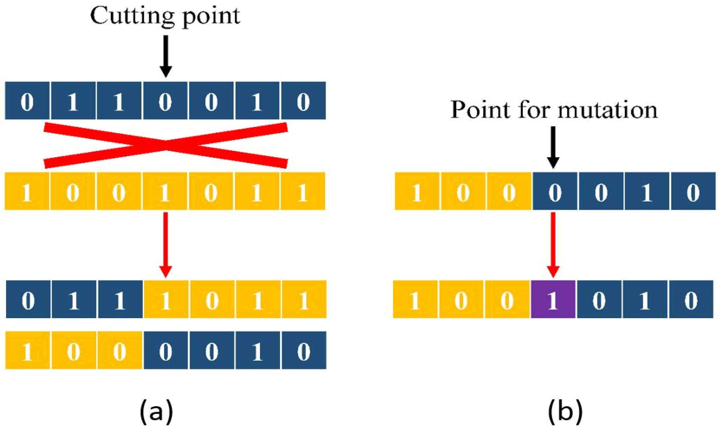
2.1.1. Standard Genetic Algorithm (SGA)
2.1.2. Particle Swarm Optimization (PSO)
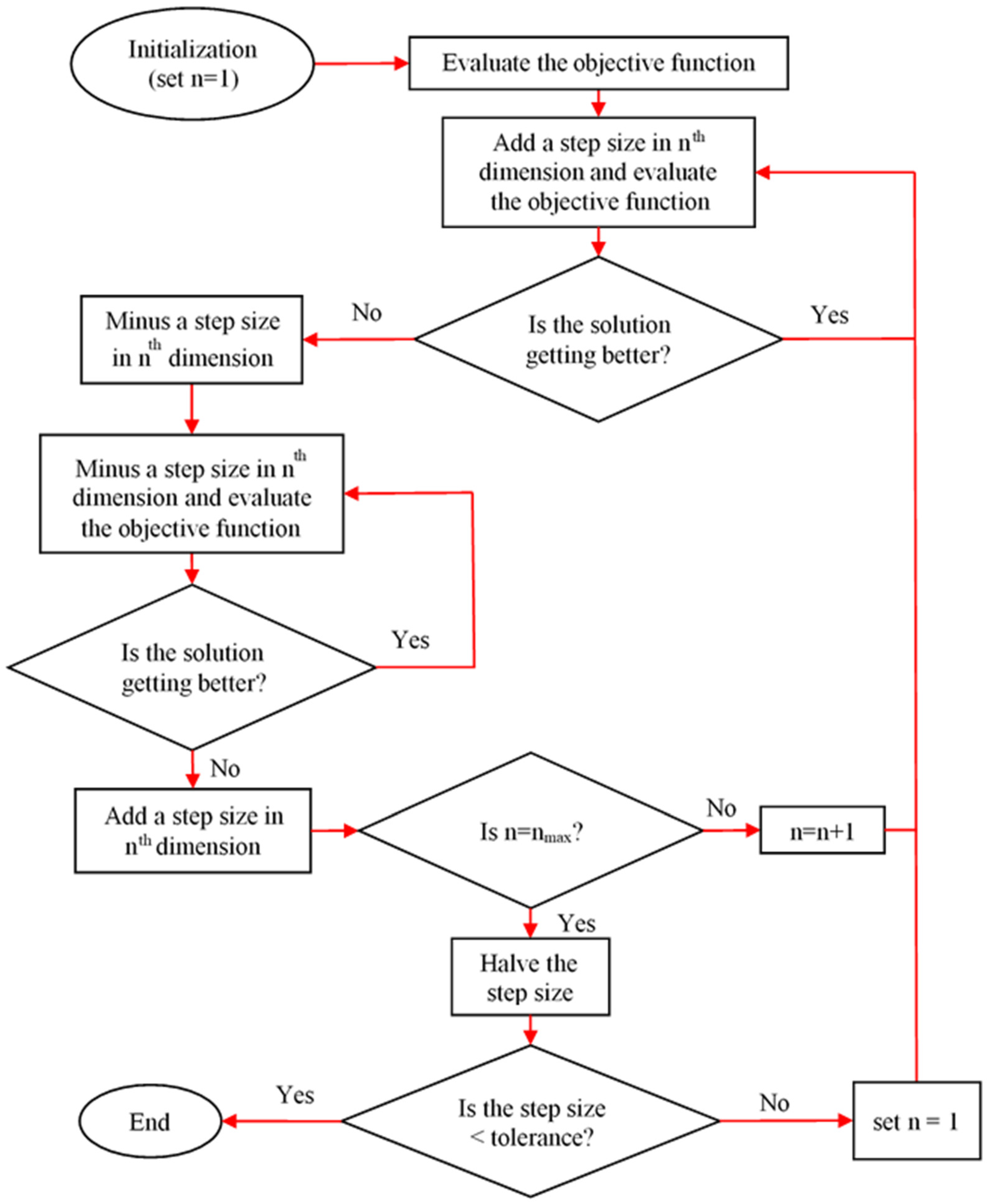
2.1.3. Pattern Search (PS)
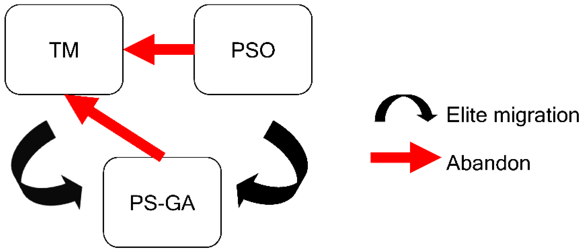
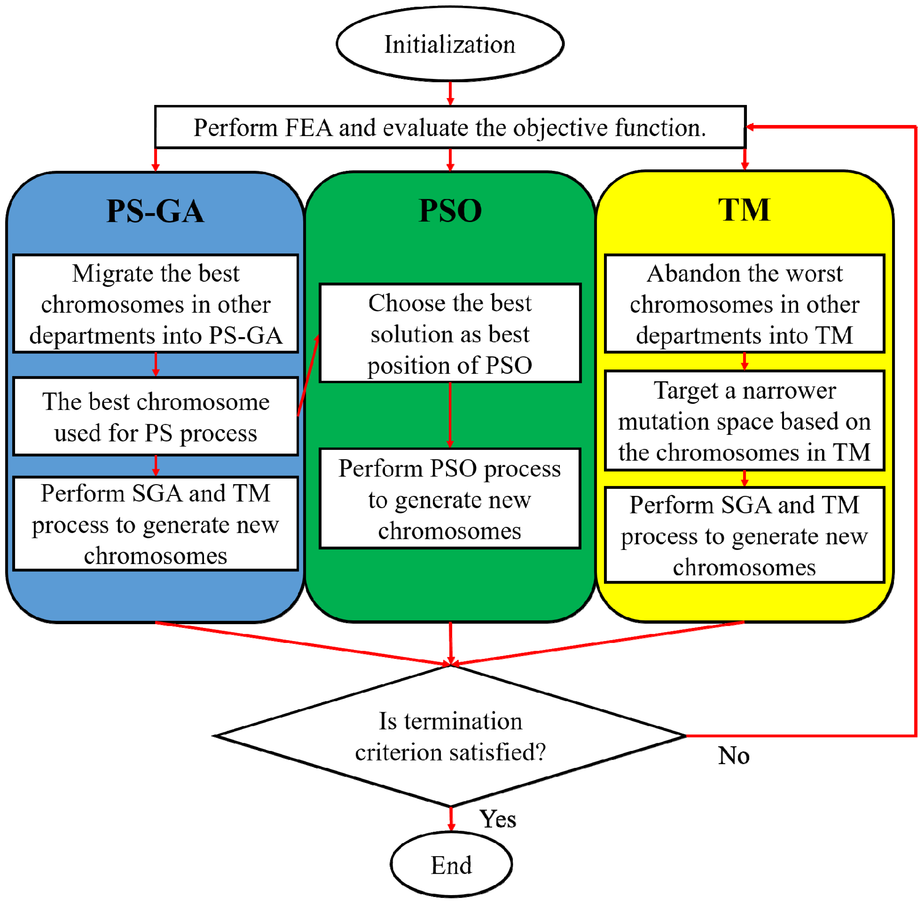
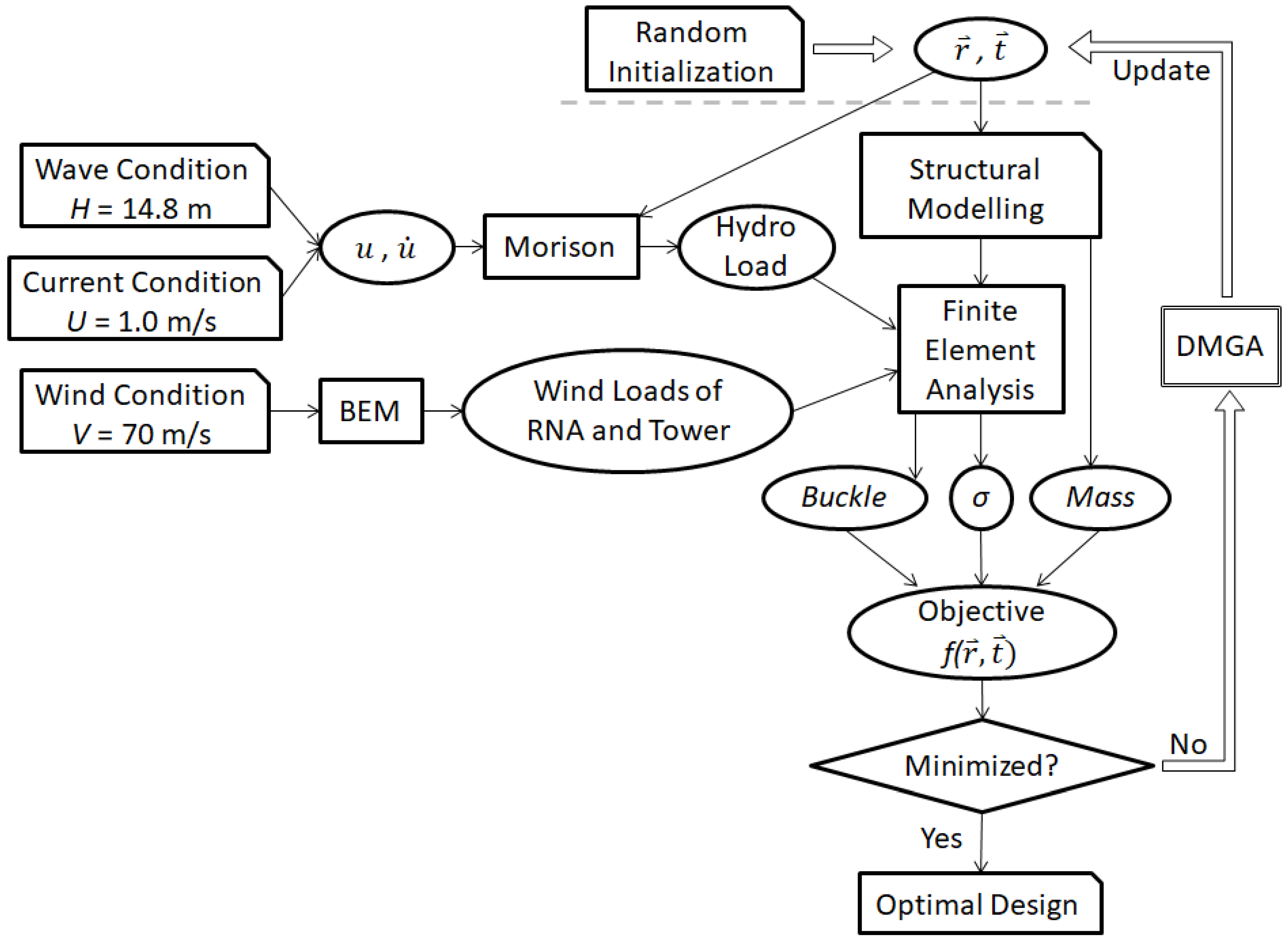
2.2. Divisional Model Genetic Algorithm (DMGA)
2.2.1. Initialization
2.2.2. SGA Operators
2.2.3. PS-GA Division
2.2.4. PSO Division
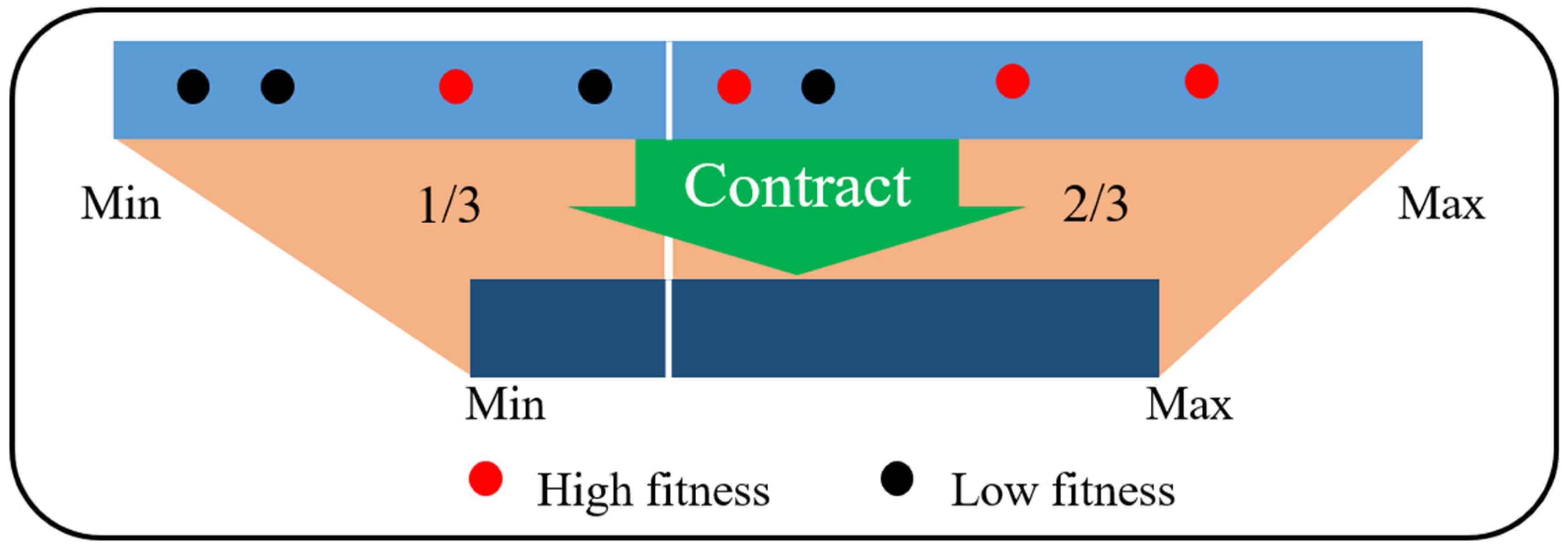
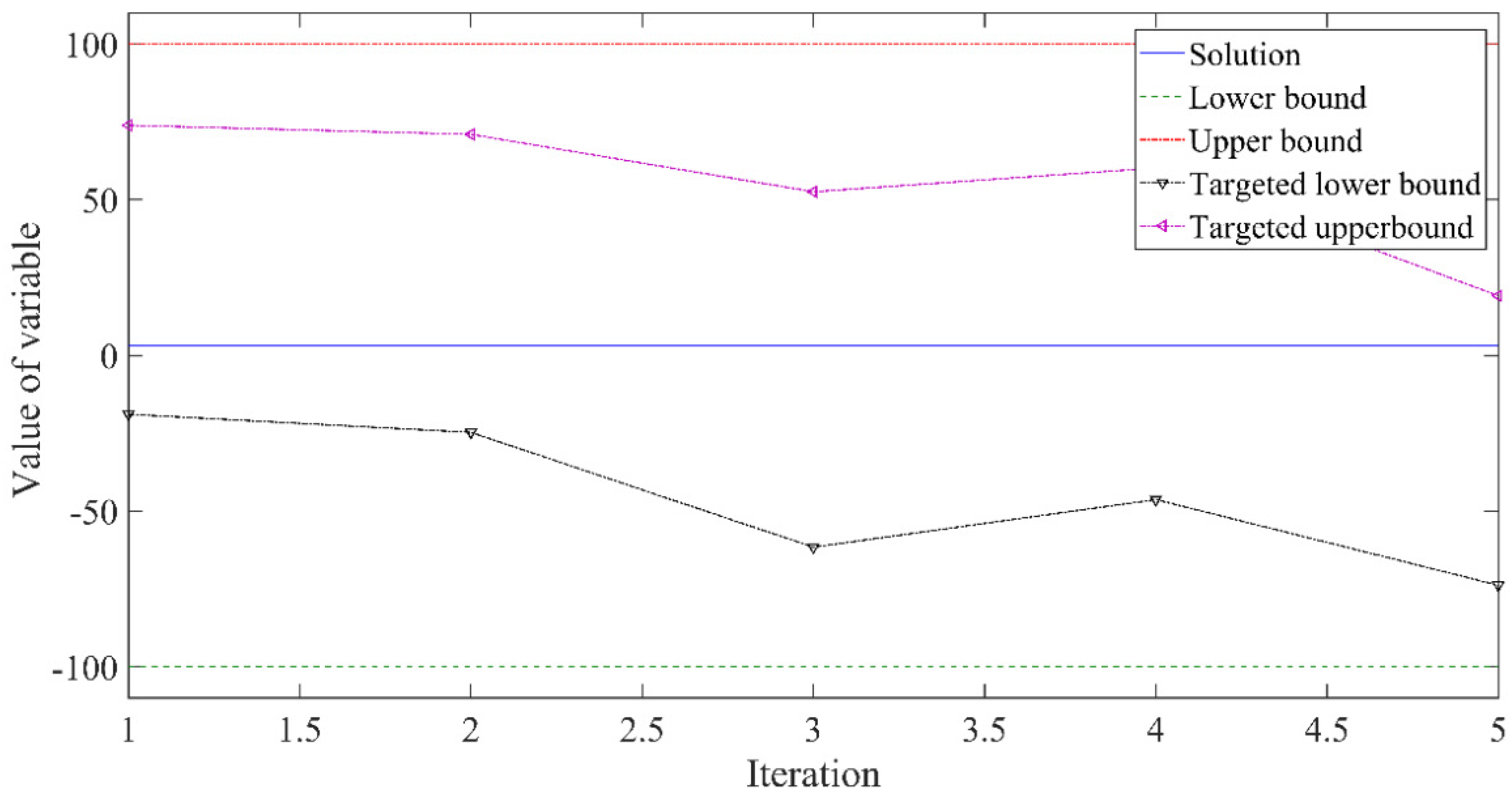
2.2.5. TM Division
3. Benchmark Study
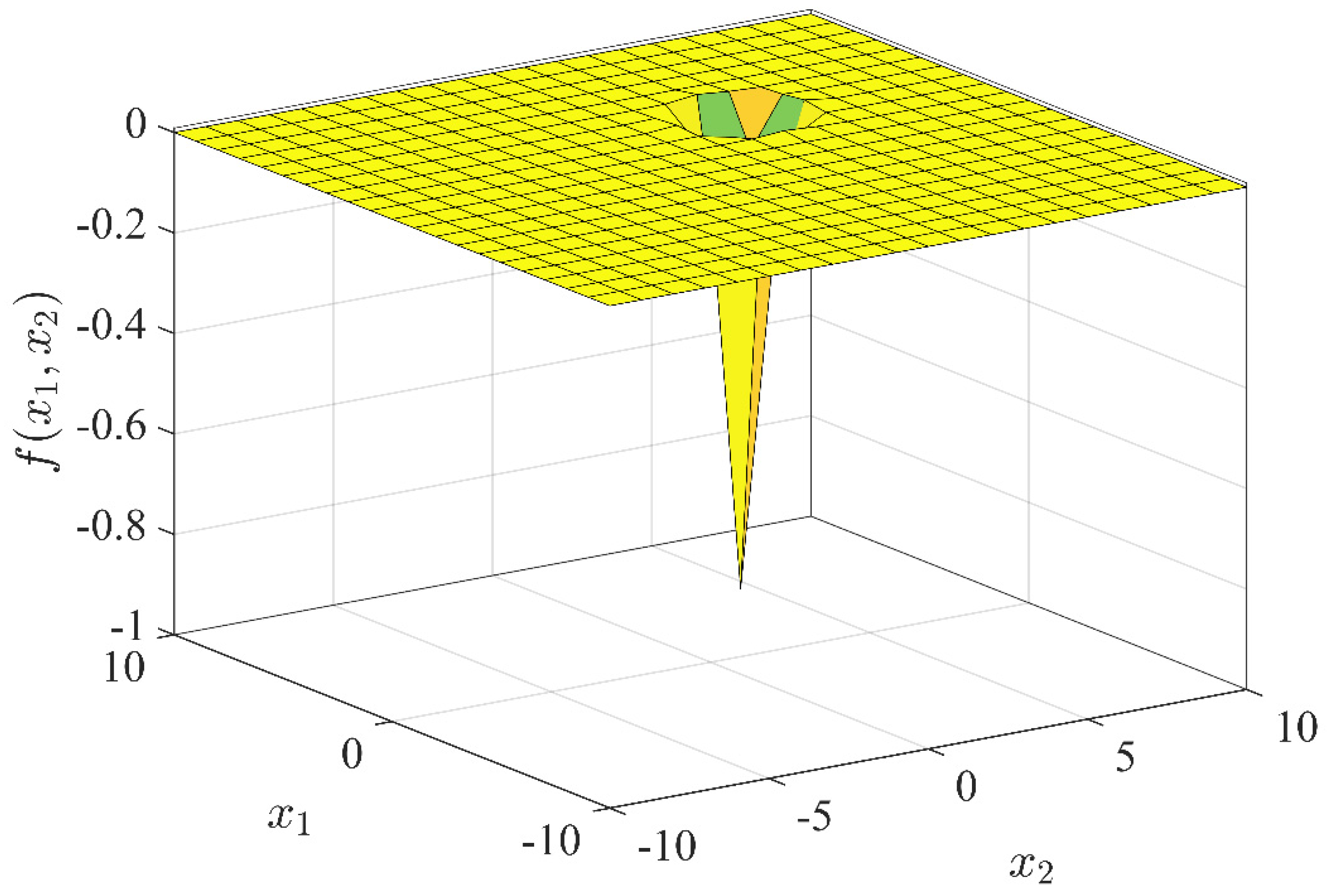
3.1. Test Functions and Algorithms Setup
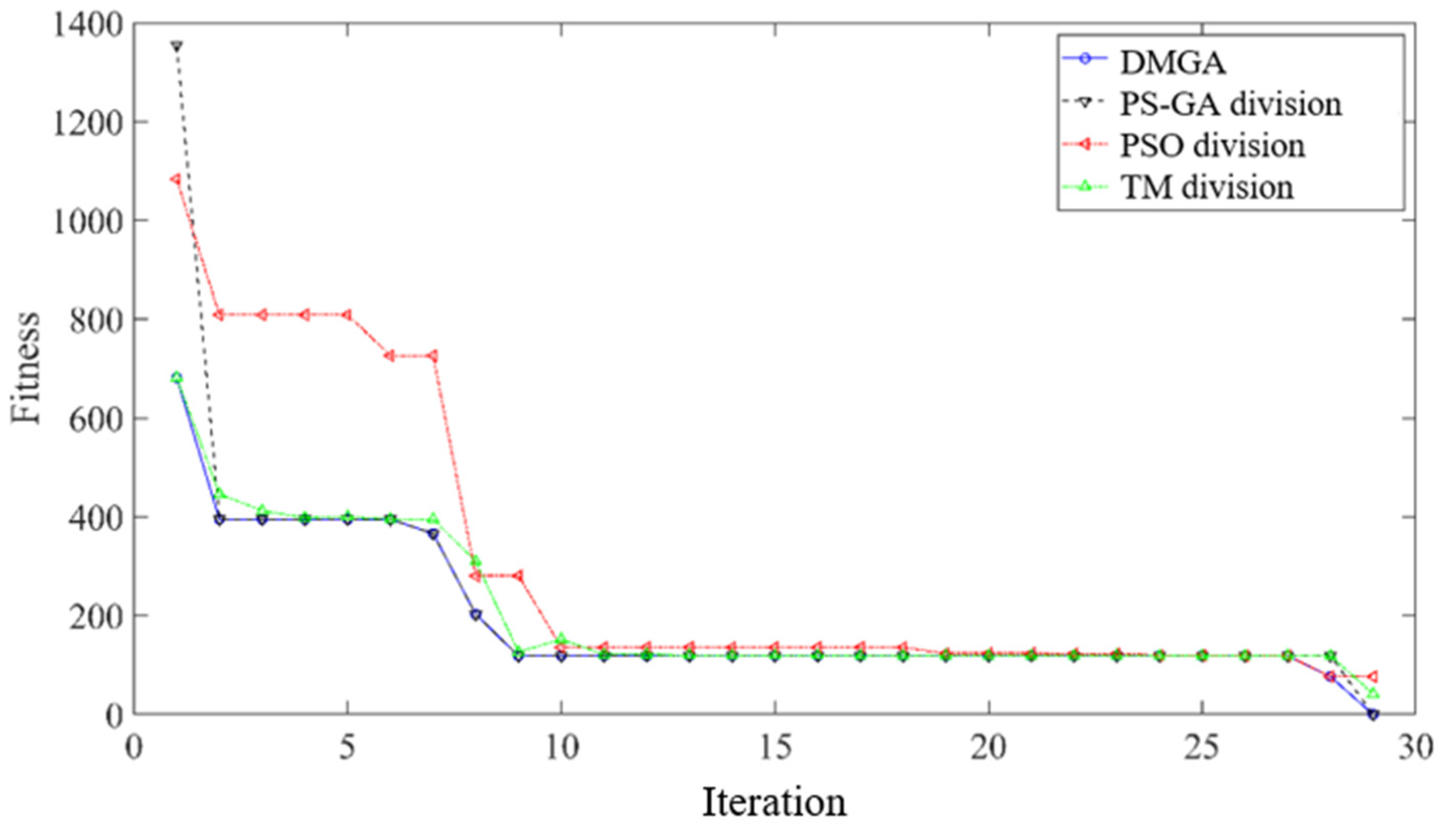
3.2. Performance Analysis
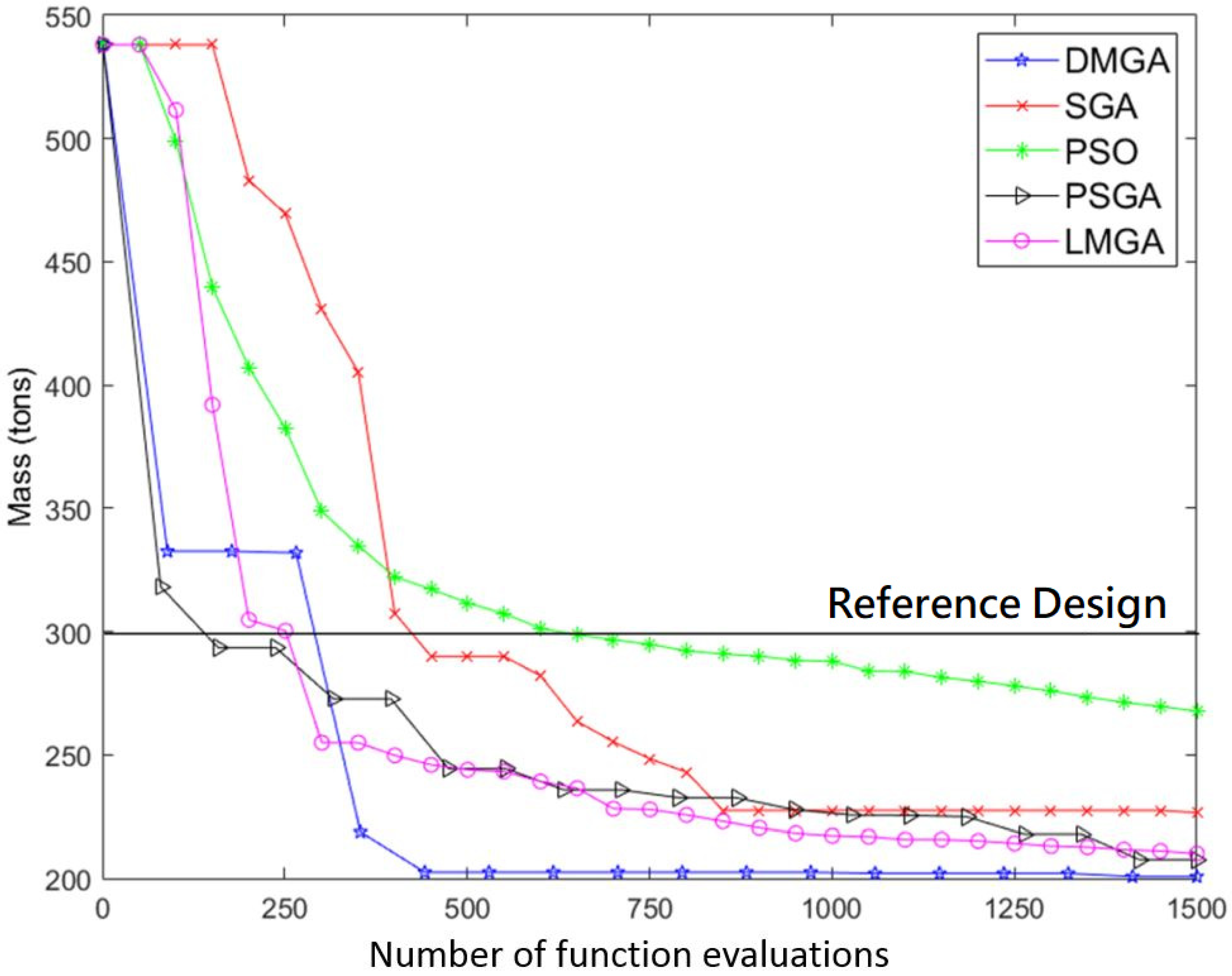
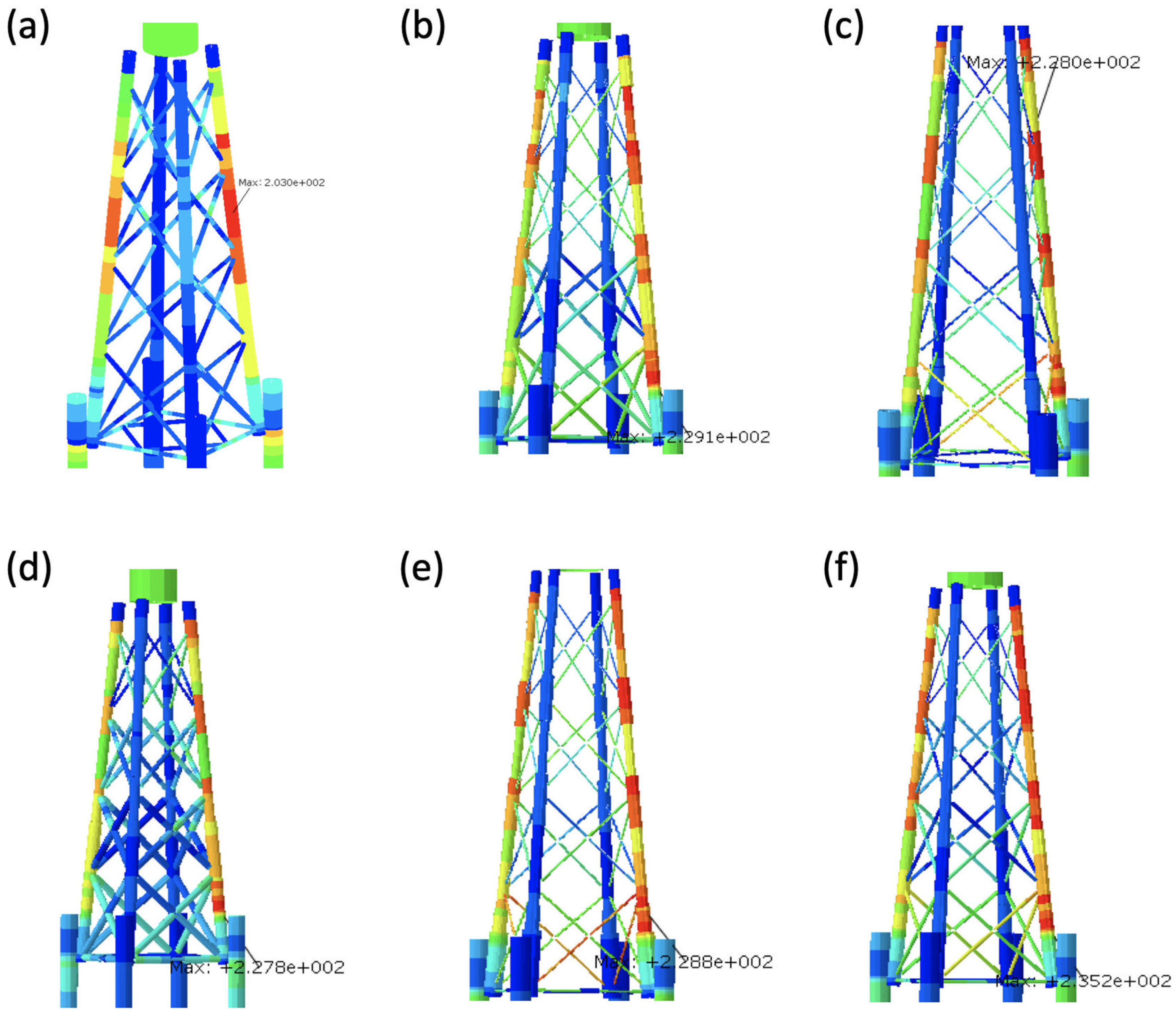
4. Jacket Substructure Optimization
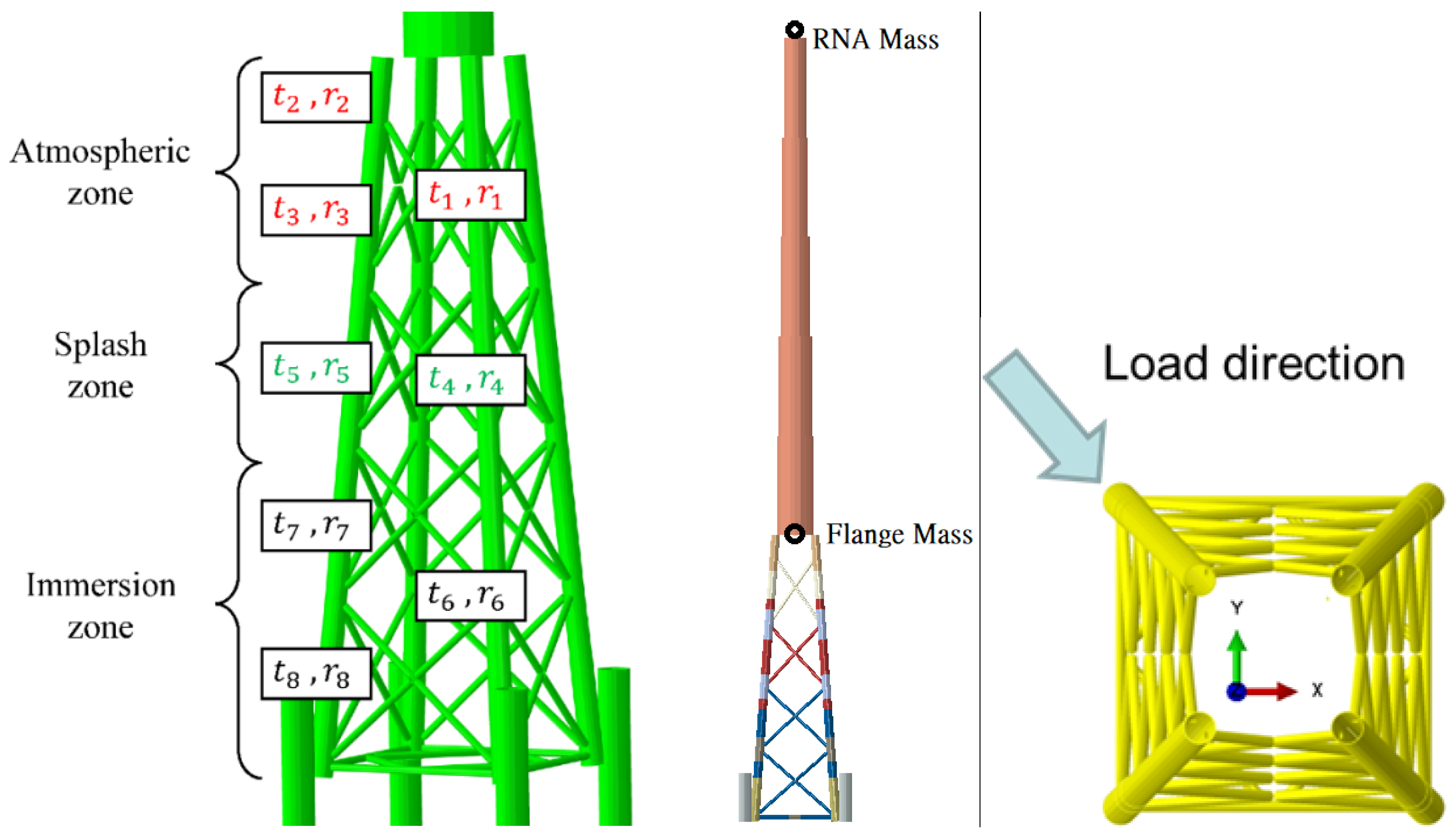
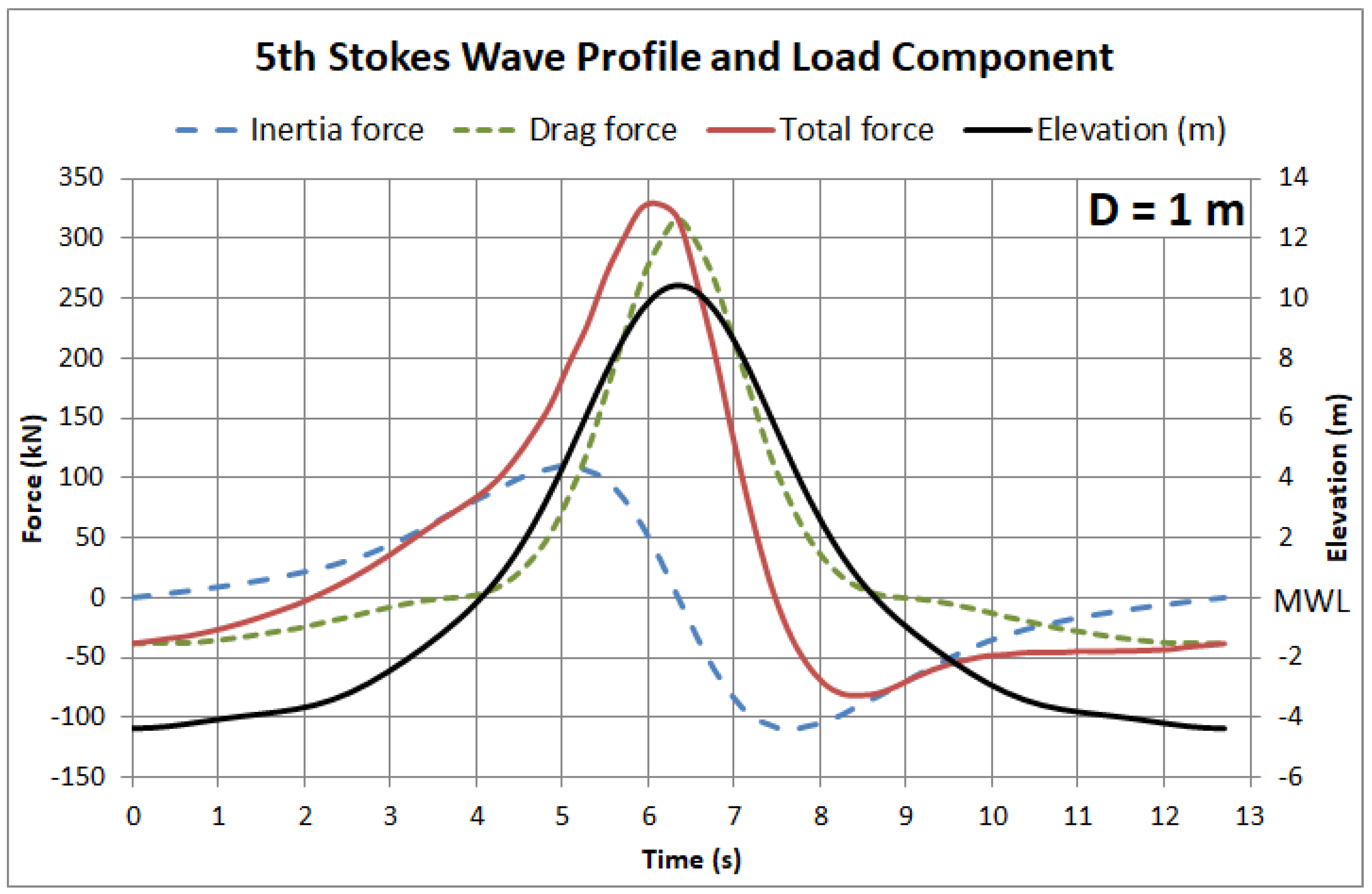
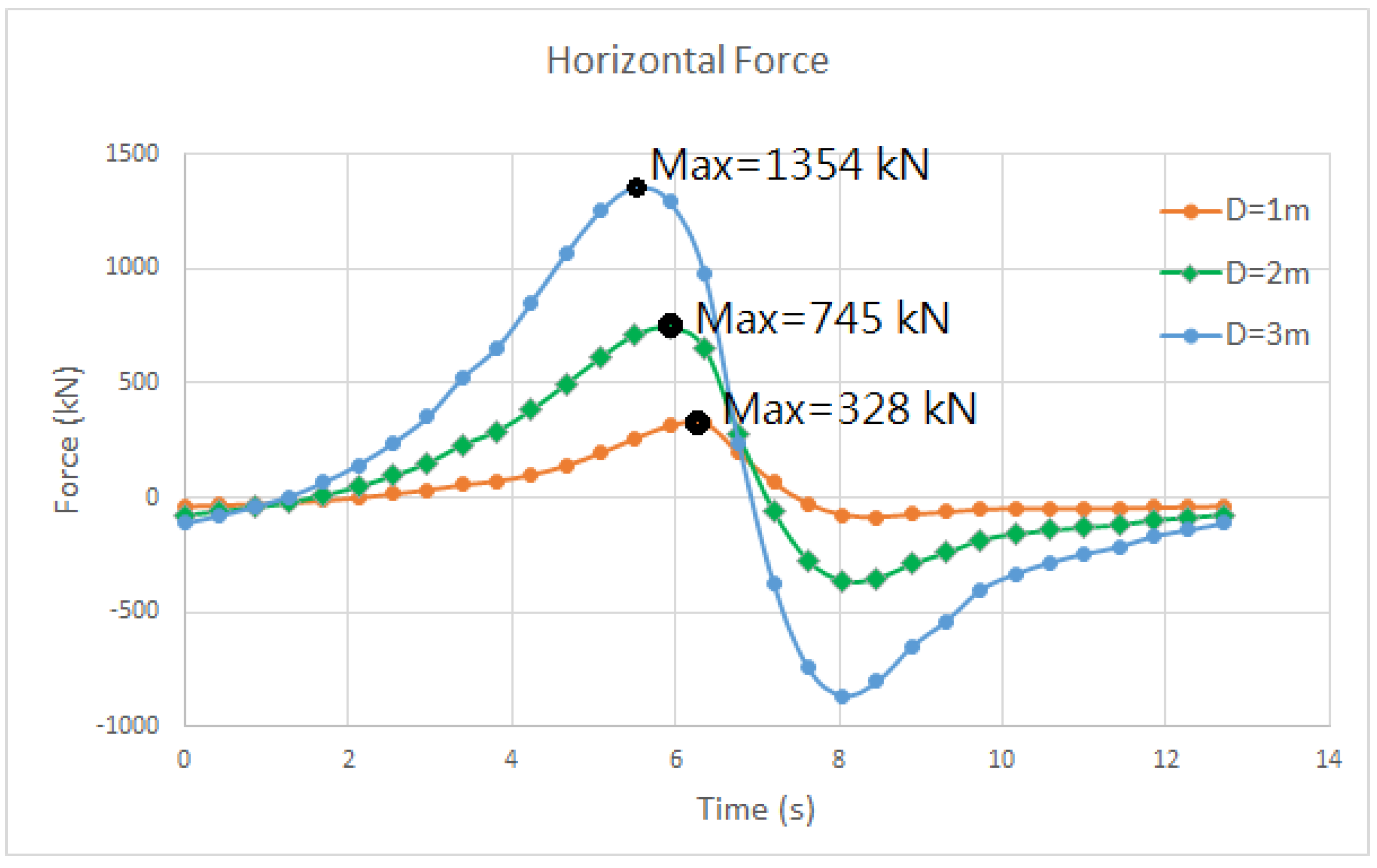
4.1. Finite Element Modelling
4.2. Algorithm Setup
4.3. Results and Discussion
5. Conclusions
Author Contributions
Funding
Conflicts of Interest
Appendix A

| Procedure of DMGA |
|---|
|
Appendix B
| Function Name | Equation | Search Range | Tolerance % | Ref. |
|---|---|---|---|---|
| Ackley D = 5 | [−32,32]D | 10−2 | [24] | |
| Schwefel D = 5 | [−500,500]D | 10−2 | [24] | |
| Rastrigin D = 10 | [−10,10]D | 10−2 | [24] | |
| De Joung D = 3 | [−5,5]D | 10−2 | [22] | |
| Rosenbrock D = 4 | [−5,10]D | 10−3 | [22] | |
| Goldstein-Price D = 2 | [−2,2]D | 10−2 | [22] | |
| Easom D = 2 | [−100,100]D | 10−2 | [22] | |
| Zakharov D = 5 | [−5,10]D | 10−3 | [22] | |
| Hartmann (H6,4) D = 6 | [0,1]D | 10−2 | [22] | |
| Eggholder D = 2 | [−512,512]D | 10−1 | [23] | |
| Schaffer D = 2 | [−100,100]D | 10−3 | [23] | |
| Styblinski-Tang D = 5 | [−5,5]D | 10−3 | [23] | |
| Beale D = 2 | [−4.5,4.5]D | 10−3 | [25] |
| Test Function | PS Step Size | PS Tolerance | ω for PSO | ||
|---|---|---|---|---|---|
| Ackley | 1 | 0.01 | 0.4 | 1 | 1 |
| Schwefel | 10 | 0.1 | 0.4 | 1 | 1 |
| Rastrigin | 1 | 0.001 | 0.8 | 1 | 1 |
| De Joung | 0.1 | 0.001 | 0.4 | 0.5 | 0.5 |
| Rosenbrock | 0.1 | 0.001 | 0.8 | 1 | 1 |
| Goldstein-Price | 0.1 | 0.001 | 0.4 | 0.5 | 0.5 |
| Easom | 10 | 0.01 | 0.4 | 1 | 1 |
| Zakharov | 1 | 0.01 | 0.4 | 1 | 1 |
| Hartman(H6,4) | 0.1 | 0.001 | 0.8 | 2 | 2 |
| Eggholder | 10 | 0.1 | 0.8 | 2 | 2 |
| Schaffer | 10 | 0.001 | 0.8 | 2 | 2 |
| Styblinski-Tang | 1 | 0.001 | 0.4 | 1 | 1 |
| Beale | 0.1 | 0.001 | 0.4 | 1 | 1 |
Appendix C
References
- Delay, T.; Jennings, T. Offshore Wind Power: Big Challenge, Big Opportunity; Carbon Trust CTC743: London, UK, 2008. [Google Scholar]
- Muskulus, M.; Schafhirt, S. Design optimization of wind turbine support structures-a review. J. Ocean Wind Energy 2014, 1, 12–22. [Google Scholar]
- Chew, K.H.; Tai, K.; Ng, E.; Muskulus, M. Optimization of offshore wind turbine support structures using an analytical gradient-based method. Energy Procedia 2015, 80, 100–107. [Google Scholar] [CrossRef] [Green Version]
- Chew, K.H.; Tai, K.; Ng, E.; Muskulus, M. Analytical gradient-based optimization of offshore wind turbine substructures under fatigue and extreme loads. Mar. Struct. 2016, 47, 23–41. [Google Scholar] [CrossRef] [Green Version]
- Pasamontes, L.B.; Torres, F.G.; Zwick, D.; Schafhirt, S.; Muskulus, M. Support structure optimization for offshore wind turbines with a genetic algorithm. In Proceedings of the ASME 2014 33rd International Conference on Ocean, Offshore and Arctic Engineering, San Francisco, California, USA, 8–13 June 2014; p. V09BTA033-V09BT09A. [Google Scholar]
- Schafhirt, S.; Zwick, D.; Muskulus, M. Reanalysis of jacket support structure for computer-aided optimization of offshore wind turbines with a genetic algorithm. In Proceedings of the The Twenty-Fourth International Ocean and Polar Engineering Conference: International Society of Offshore and Polar Engineers, Busan, Korea, 15–20 June 2014. [Google Scholar]
- AlHamaydeh, M.; Barakat, S.; Nasif, O. Optimization of Support Structures for Offshore Wind Turbines Using Genetic Algorithm with Domain-Trimming. Math. Probl. Eng. 2017, 2017, 5978375. [Google Scholar] [CrossRef] [Green Version]
- Gentils, T.; Wang, L.; Kolios, A. Integrated structural optimisation of offshore wind turbine support structures based on finite element analysis and genetic algorithm. Appl. Energy 2017, 199, 187–204. [Google Scholar] [CrossRef] [Green Version]
- Kaveh, A.; Sabeti, S. Structural optimization of jacket supporting structures for offshore wind turbines using colliding bodies optimization algorithm. Struct. Design Tall Spec. Build. 2018, 27, e1494. [Google Scholar] [CrossRef]
- Chehouri, A.; Younes, R.; Ilinca, A.; Perron, J. Review of performance optimization techniques applied to wind turbines. Appl. Energy 2015, 142, 361–388. [Google Scholar] [CrossRef]
- Hofmeister, B.; Bruns, M.; Rolfes, R. Finite element model updating using deterministic optimisation: A global pattern search approach. Eng. Struct. 2019, 195, 373–381. [Google Scholar] [CrossRef]
- Li, F.; Lam, K.Y.; Wang, L. Power allocation in cognitive radio networks over Rayleigh-fading channels with hybrid intelligent algorithms. Wirel. Netw. 2018, 24, 2397–2407. [Google Scholar] [CrossRef]
- Sahu, R.K.; Panda, S.; Sekhar, G.C. A novel hybrid PSO-PS optimized fuzzy PI controller for AGC in multi area interconnected power systems. Int. J. Electr. Power Energy Syst. 2015, 64, 880–893. [Google Scholar] [CrossRef]
- Gandomkar, M.; Vakilian, M.; Ehsan, M.A. Combination of genetic algorithm and simulated annealing for optimal DG allocation in distribution networks. In Proceedings of the Canadian Conference on Electrical and Computer Engineering, Saskatoon, SA, Canada, 1–4 May 2005; pp. 645–648. [Google Scholar]
- Pourvaziri, H.; Naderi, B. A hybrid multi-population genetic algorithm for the dynamic facility layout problem. Appl. Soft Comput. 2014, 24, 457–469. [Google Scholar] [CrossRef]
- Krink, T.; Løvbjerg, M. The lifecycle model: Combining particle swarm optimisation, genetic algorithms and hillclimbers. In International Conference on Parallel Problem Solving from Nature—PPSN VII. PPSN 2002. Lecture Notes in Computer Science; Springer: Berlin/Heidelberg, Germany, 2002; Volume 2439, pp. 621–630. [Google Scholar]
- Turing, A.M. Computing machinery and intelligence. Mind 1950, 59, 433–460. [Google Scholar] [CrossRef]
- Holland, J.H. Adaptation in natural and artificial systems. In An Introductory Analysis with Application to Biology, Control, and Artificial Intelligence; University of Michigan Press: Ann Arbor, MI, USA, 1975. [Google Scholar]
- Xing, L.N.; Chen, Y.W.; Cai, H.P. An intelligent genetic algorithm designed for global optimization of multi-minima functions. Appl. Math. Comput. 2006, 178, 355–371. [Google Scholar] [CrossRef]
- Kennedy, J. Particle swarm optimization. In Encyclopedia of Machine Learning; Springer: Berlin/Heidelberg, Germany, 1995; pp. 760–766. [Google Scholar]
- Shi, Y.; Eberhart, R. A modified particle swarm optimizer. In Proceedings of the Evolutionary Computation Proceedings, 1998 IEEE World Congress on Computational Intelligence, Anchorage, AK, USA, 4–9 May 1998; pp. 69–73. [Google Scholar]
- Hooke, R.; Jeeves, T.A. “Direct Search” solution of numerical and statistical problems. J. ACM (JACM) 1961, 8, 212–229. [Google Scholar] [CrossRef]
- Chelouah, R.; Siarry, P. Tabu search applied to global optimization. Eur. J. Oper. Res. 2000, 123, 256–270. [Google Scholar] [CrossRef]
- Mishra, S.K. Some new test functions for global optimization and performance of repulsive particle swarm method. SSRN Electron. J. 2006, 1–24. [Google Scholar] [CrossRef] [Green Version]
- Liang, J.J.; Qu, B.Y.; Suganthan, P.N.; Hernández-Díaz, A.G. Problem Definitions and Evaluation Criteria for the CEC 2013 Special Session on Real-Parameter Optimization; Technical Report; Computational Intelligence Laboratory, Zhengzhou University: Zhengzhou, China; Nanyang Technological University: Singapore, 2013; Volume 201212, pp. 3–18. [Google Scholar]
- Beale, E. On an Iterative Method for Finding a Local Minimum of a Function of More than One Variable; Technical Report 25; Princeton University, Statistical Techniques Research Group: Princeton, NJ, USA, 1958. [Google Scholar]
- Juang, C.F. A hybrid of genetic algorithm and particle swarm optimization for recurrent network design. IEEE Trans. Syst. Man Cybern. Part B (Cybern.) 2004, 34, 997–1006. [Google Scholar] [CrossRef] [PubMed]
- Häfele, J. A Numerically Efficient and Holistic Approach to Design Optimization of Offshore wind Turbine Jacket Substructures. Ph.D. Thesis, Gottfried Wilhelm Leibniz Universität, Hanover, Germany, 2019. [Google Scholar]
- Development Plan of Wind Power in Taiwan (English Translation of Chinese Title). Available online: https://energywhitepaper.tw/upload/201712/151376189216283.pdf (accessed on 29 May 2020).
- International Electrotechnical Commission (IEC). IEC 61400-3 Part 3: Design Requirements for Offshore Wind Turbines; IEC: Geneva, Switzerland, 2009. [Google Scholar]
- Det Norske Veritas and Germanischer Lloyd (DNVGL). Loads and Site Conditions for Wind Turbines; DNVGL-ST-0437; DNVGL: Oslo, Norway, 2016. [Google Scholar]
- Jonkman, J.; Butterfield, S.; Musial, W.; Scott, G. Definition of a 5-MW Reference Wind Turbine for Offshore System Development; NREL/TP-500-38060; National Renewable Energy Lab (NREL): Golden, CO, USA, 2009. [Google Scholar]
- Offshore Wind Power Demonstration Incentive Program–Annex 3: Requirements of Specification (English Translation of Chinese Title). Available online: https://law.moj.gov.tw/LawClass/LawAll.aspx?pcode=J0130063 (accessed on 29 May 2020).
- Morison, J.; Johnson, J.; Schaaf, S. The force exerted by surface waves on piles. J. Pet. Technol. 1950, 2, 149–154. [Google Scholar] [CrossRef]
- Chakrabarti, S.K. Hydrodynamics of Offshore Structures; WIT Press: Southampton, UK, 1987. [Google Scholar]
- Constrained Optimization—Wikipedia. Available online: https://en.wikipedia.org/wiki/Constrained_optimization (accessed on 29 May 2020).
- Standards Norway. NORSOK Standard N-004 Design of Steel Structures; Standards Norway: Lysaker, Norway, 2004. [Google Scholar]


| Algorithm | DMGA | SGA | PSO | PSGA | PSPSO | HGAPSO | LMGA | |
|---|---|---|---|---|---|---|---|---|
| Function | Effectiveness 1 | |||||||
| Efficiency 2 | ||||||||
| Ackley | 100 | 0 | 56 | 68 | 100 | 91 | 99 | |
| 5380 | 0 | 1451 | 252,278 | 1891 | 219,310 | 13,040 | ||
| Schwefel | 100 | 100 | 6 | 100 | 2 | 100 | 100 | |
| 1722 | 175,399 | 1330 | 34,476 | 195 | 48,414 | 22,643 | ||
| Rastrigin | 100 | 0 | 0 | 71 | 100 | 0 | 0 | |
| 3197 | 0 | 0 | 203,757 | 4389 | 0 | 0 | ||
| De Joung | 100 | 100 | 100 | 100 | 100 | 100 | 100 | |
| 183 | 3434 | 395 | 192 | 194 | 686 | 419 | ||
| Rosenbrock | 99 | 1 | 67 | 2 | 79 | 100 | 98 | |
| 35,237 | 320,580 | 8424 | 235,324 | 10,072 | 64,466 | 154,925 | ||
| Goldstein-Price | 100 | 100 | 100 | 100 | 100 | 100 | 100 | |
| 446 | 3365 | 482 | 643 | 527 | 1259 | 524 | ||
| Easom | 100 | 100 | 99 | 100 | 95 | 100 | 100 | |
| 962 | 11,912 | 7244 | 3284 | 1608 | 6288 | 1909 | ||
| Zakharov | 100 | 0 | 13 | 3 | 100 | 95 | 99 | |
| 10,370 | 0 | 1209 | 507,315 | 2251 | 265,632 | 57,163 | ||
| Hartman (H6,4) | 80 | 96 | 6 | 98 | 54 | 40 | 56 | |
| 7502 | 161,007 | 136,880 | 65,964 | 836 | 32,072 | 84,422 | ||
| Eggholder | 64 | 86 | 0 | 72 | 8 | 49 | 97 | |
| 90,029 | 164,835 | 0 | 164,080 | 25,302 | 66,124 | 106,781 | ||
| Schaffer | 84 | 93 | 0 | 95 | 27 | 31 | 24 | |
| 118,778 | 188,019 | 0 | 159,428 | 56,886 | 74,706 | 286,874 | ||
| Styblinski-Tang | 100 | 42 | 16 | 99 | 12 | 100 | 100 | |
| 738 | 387,744 | 1084 | 35,968 | 242 | 26,356 | 13,725 | ||
| Beale | 100 | 100 | 89 | 100 | 94 | 100 | 100 | |
| 729 | 3775 | 537 | 2484 | 624 | 6559 | 749 | ||
| Algorithm | DMGA | SGA | PSO | PSGA | PSPSO | HGAPSO | LMGA | |
|---|---|---|---|---|---|---|---|---|
| Function | Rank | |||||||
| Ackley | 2 | 7 | 6 | 5 | 1 | 4 | 3 | |
| Schwefel | 1 | 5 | 6 | 3 | 7 | 4 | 2 | |
| Rastrigin | 1 | 4 | 4 | 3 | 2 | 4 | 4 | |
| De Joung | 1 | 7 | 4 | 2 | 3 | 6 | 5 | |
| Rosenbrock | 2 | 7 | 5 | 6 | 4 | 1 | 3 | |
| Goldstein-Price | 1 | 7 | 2 | 5 | 4 | 6 | 3 | |
| Easom | 1 | 5 | 6 | 3 | 7 | 4 | 2 | |
| Zakharov | 2 | 7 | 5 | 6 | 1 | 4 | 3 | |
| Hartman (H6,4) | 3 | 2 | 7 | 1 | 5 | 6 | 4 | |
| Eggholder | 4 | 2 | 7 | 3 | 6 | 5 | 1 | |
| Schaffer | 3 | 2 | 7 | 1 | 5 | 4 | 6 | |
| Styblinski-Tang | 1 | 5 | 6 | 4 | 7 | 3 | 2 | |
| Beale | 1 | 4 | 6 | 3 | 6 | 5 | 2 | |
| Avg. Rank | 1.77 | 4.92 | 5.46 | 3.46 | 4.46 | 4.31 | 3.08 | |
| Mean Wind Speed | Gust Factor | Gust Wind | Wave Height | Wave Period | Wave Length |
|---|---|---|---|---|---|
| 50 m/s | 1.4 | 70 m/s | 14.8 m | 12.7 s | 197 m |
| PS Step Size | PS Tolerance | ω for PSO | ||
|---|---|---|---|---|
| 80/6 1 | 20/1.5 1 | 1 | 1 | 0.5 |
| Algorithm | DMGA | SGA | PSO | PSGA | LMGA | Reference | |
|---|---|---|---|---|---|---|---|
| Member | Thickness (mm) | ||||||
| Radius (mm) | |||||||
| Atmospheric brace | 7.2 | 14 | 7.4 | 12 | 14.5 | 18.9 | |
| 100 | 100 | 165 | 100 | 101 | 203 | ||
| Atmospheric upper leg | 43.4 | 49 | 33.9 | 45 | 41.7 | 42.5 | |
| 463 | 447 | 673 | 463 | 513 | 600 | ||
| Atmospheric lower leg | 49 | 49 | 48.9 | 56 | 40 | 42.5 | |
| 390 | 492 | 557 | 363 | 450 | 600 | ||
| Splash brace | 6 | 12 | 18.6 | 6 | 16.6 | 12.8 | |
| 106 | 93 | 277 | 100 | 143 | 226 | ||
| Splash leg | 27.2 | 30.9 | 34.1 | 28 | 32.2 | 34 | |
| 569 | 527 | 521 | 566 | 510 | 600 | ||
| Immersion brace | 10.6 | 9 | 10 | 7 | 6 | 18.9 | |
| 119 | 115 | 387 | 124 | 173 | 203 | ||
| Immersion upper leg | 36.7 | 48 | 28.1 | 42 | 34.9 | 42.5 | |
| 565 | 461 | 674 | 507 | 580 | 600 | ||
| Immersion lower leg | 33 | 62 | 58.5 | 33 | 41.8 | 67.5 | |
| 837 | 546 | 611 | 837 | 644 | 650 | ||
| Mass (ton) | 200 | 226 | 267 | 207 | 209 | 300 | |
| Converged iterations | 400 | 850 | over 1500 | 1420 | 1400 | - | |
| Maximum stress (MPa) | 229 | 228 | 228 | 229 | 235 | 203 | |
| Member of maximum stress | Immersion lower leg | Atmospheric upper leg | Immersion lower leg | Immersion lower leg | Immersion lower leg | Splash leg | |
© 2020 by the authors. Licensee MDPI, Basel, Switzerland. This article is an open access article distributed under the terms and conditions of the Creative Commons Attribution (CC BY) license (http://creativecommons.org/licenses/by/4.0/).
Share and Cite
Liu, D.-P.; Lin, T.-Y.; Huang, H.-H. Improving the Computational Efficiency for Optimization of Offshore Wind Turbine Jacket Substructure by Hybrid Algorithms. J. Mar. Sci. Eng. 2020, 8, 548. https://doi.org/10.3390/jmse8080548
Liu D-P, Lin T-Y, Huang H-H. Improving the Computational Efficiency for Optimization of Offshore Wind Turbine Jacket Substructure by Hybrid Algorithms. Journal of Marine Science and Engineering. 2020; 8(8):548. https://doi.org/10.3390/jmse8080548
Chicago/Turabian StyleLiu, Ding-Peng, Tsung-Yueh Lin, and Hsin-Haou Huang. 2020. "Improving the Computational Efficiency for Optimization of Offshore Wind Turbine Jacket Substructure by Hybrid Algorithms" Journal of Marine Science and Engineering 8, no. 8: 548. https://doi.org/10.3390/jmse8080548