Capturing the Variability in Instantaneous Vehicle Emissions Based on Field Test Data


Department of Civil & Mineral Engineering, University of Toronto, 35 St George St, Toronto, ON M5S 1A4, Canada
*
Author to whom correspondence should be addressed.
Atmosphere 2020, 11(7), 765; https://doi.org/10.3390/atmos11070765
Submission received: 25 May 2020
/
Revised: 7 July 2020
/
Accepted: 15 July 2020
/
Published: 20 July 2020
(This article belongs to the Special Issue Emissions, Transport and Fate of Pollutants in the Atmosphere)
Abstract
:Emission models are important tools for traffic emission and air quality estimates. Existing instantaneous emission models employ the steady-state “engine emissions map” to estimate emissions for individual vehicles. However, vehicle emissions vary significantly, even under the same driving conditions. Variability in the emissions at a specific driving condition depends on various influencing factors. It is important to gain insight into the effects of these factors, to enable detailed modeling of individual vehicle emissions. This study employs a portable emissions measurement system (PEMS), to collect vehicle emissions including the corresponding parameters of engine condition, vehicle activity, catalyst temperature, geography, and meteorology, to analyze the variability in emission rates as a function of those factors, across different vehicle specific power (VSP) categories. We observe that carbon dioxide, carbon monoxide, nitrogen oxides, and particle number emissions are strongly correlated with engine parameters (engine speed, torque, load, and air-fuel ratio) and vehicle activity parameters (vehicle speed and acceleration). In the same VSP bin, emissions per second on highways and ramps are higher than those on arterial roads, and the emissions when the vehicle is traveling downhill tend to be higher than the emissions during uphill traveling, because of higher observed speeds and accelerations. Morning emissions are higher than afternoon emissions, due to lower temperatures.
1. Introduction
Emission models are important tools for traffic emission and air quality estimates. Certain operational emission models collect emissions and the corresponding engine parameters (e.g., engine speed, torque, power, and air-fuel ratio) to develop a steady-state “engine emissions map” for each vehicle type. In practice, it is difficult to obtain sufficient engine data to develop a high-resolution engine map. Alternatively, some models employ vehicle activity parameters such as vehicle speed, acceleration, and vehicle specific power (VSP) [1] to explain emissions. Table 1 lists some of the operating emission models. They are categorized based on models that use engine operation data and models that use vehicle activity data. These models calculate average emissions per unit of time, known as emission rates, for different vehicle types and driving conditions, relying on large databases of emission test results (dynamometer and on-road). The emission rates are further used to generate emission inventories at the regional level or the link level for a fleet of vehicles with averaging periods ranging from one hour to one year.
In recent years, research into approaches for modelling second by second emissions of individual vehicles has gained momentum, primarily driven by the needs of planners and policy-makers to generate accurate estimates of vehicle emissions to support project-level analysis, as well as regional emission inventories. Studies have indicated that there are significant differences between measured and predicted emissions for individual vehicles [13]. This can be expected, because the emission rates embedded in the emission models are calculated by averaging the emissions of multiple vehicles. For instance, the emission rates in the Motor Vehicle Emissions Simulator (MOVES) model developed by the US Environmental Protection Agency (EPA) are based on data from 2.3 million tests from over 500,000 vehicles [14]. It is not reasonable to compare the emission rates of one specific vehicle with emission rates that are meant to represent the entire fleet.
The emission modeling process is complex, especially when it comes to estimating instantaneous emissions for an individual vehicle, owing to the various parameters affecting emissions. In addition to engine operation and vehicle activity, collecting real-world vehicle emission data introduces a number of external factors, which reduces the ability to produce robust results [15]. For light-duty gasoline vehicles, typically, three categories of external factors have significant effects on their emissions, these include: emission control technology, geography (e.g., altitude, road type, and road grade), and meteorology (e.g., ambient temperature). Among these factors, emission control causes a variation in the emissions of carbon monoxide (CO), hydrocarbons (HC), nitrogen oxides (NOx), and particulate matter (PM)/particle number (PN), depending on the operation of control technology. Geography and meteorology factors both have significant effects on engine operation, vehicle activity, and/or emission control.
It is important to gain insight into the effects of these factors on vehicle emissions, to allow for the detailed modeling of individual vehicle emissions. One of the proposed methods is by capturing the variability in instantaneous vehicle emissions based on field test data. Many studies made efforts to validate the effects of altitude, road type, road grade, and ambient temperature on emissions, in order to correct the errors of emission estimates related to these factors. Frey et al. [16,17] and Nagpure et al. [18] indicated that altitude and road grade are the dominant factors influencing the emissions of CO and NOx in hilly areas. Wyatt et al. [19] points out that it is incorrect to assume that the increase in emissions on uphill sections will be offset by the decrease in emissions on paired downhill sections. Multiple studies [20,21,22,23,24] reported that positive road grade tends to increase vehicle emissions per distance, if the vehicles are traveling at a similar speed, and the effects vary by pollutant. De Vlieger et al. [25] and Jackson et al. [26] reported that CO2, CO, HC, NOx, and PN emissions are all systematically related to road type. The authors observed that the emissions for restricted access roads (like expressways) are significantly different from the emissions for unrestricted access roads (like arterial roads). Nagpure et al. [18] indicated that CO tends to increase at high altitude and high ambient temperature, while the opposite trend is observed for NOx. Ko et al. [27] explained that as the ambient temperature decreases, because of the poor mixing of fuel and air and the reduced combustion efficiency and stability, the exhaust gas recirculation rates decrease, increasing the NOx emissions. Most of these studies modeled emissions as a function of vehicle speed and acceleration instead of VSP, although the latter is one of the most important parameters often used to explain vehicle emissions in current operational emission models.
This study employs portable emissions measurement systems (PEMS) to collect vehicle emissions, and other parameters to explore the variability of emissions across different VSP categories, as a function of engine speed, torque, load, air-fuel ratio, vehicle speed, acceleration, altitude, road grade, road type, catalyst temperature, ambient temperature, and time of day. Capturing and understanding the variability in emissions under VSP categories provides critical information for the development of instantaneous emission models. Since VSP plays an important role in predicting emissions, by capturing and explaining the variability in emissions under each VSP category, this study informs the development of emission modelling tools in terms of the VSP resolution and the impacts of different factors on the range of emissions per VSP category.
2. Methodology
2.1. Data Collection
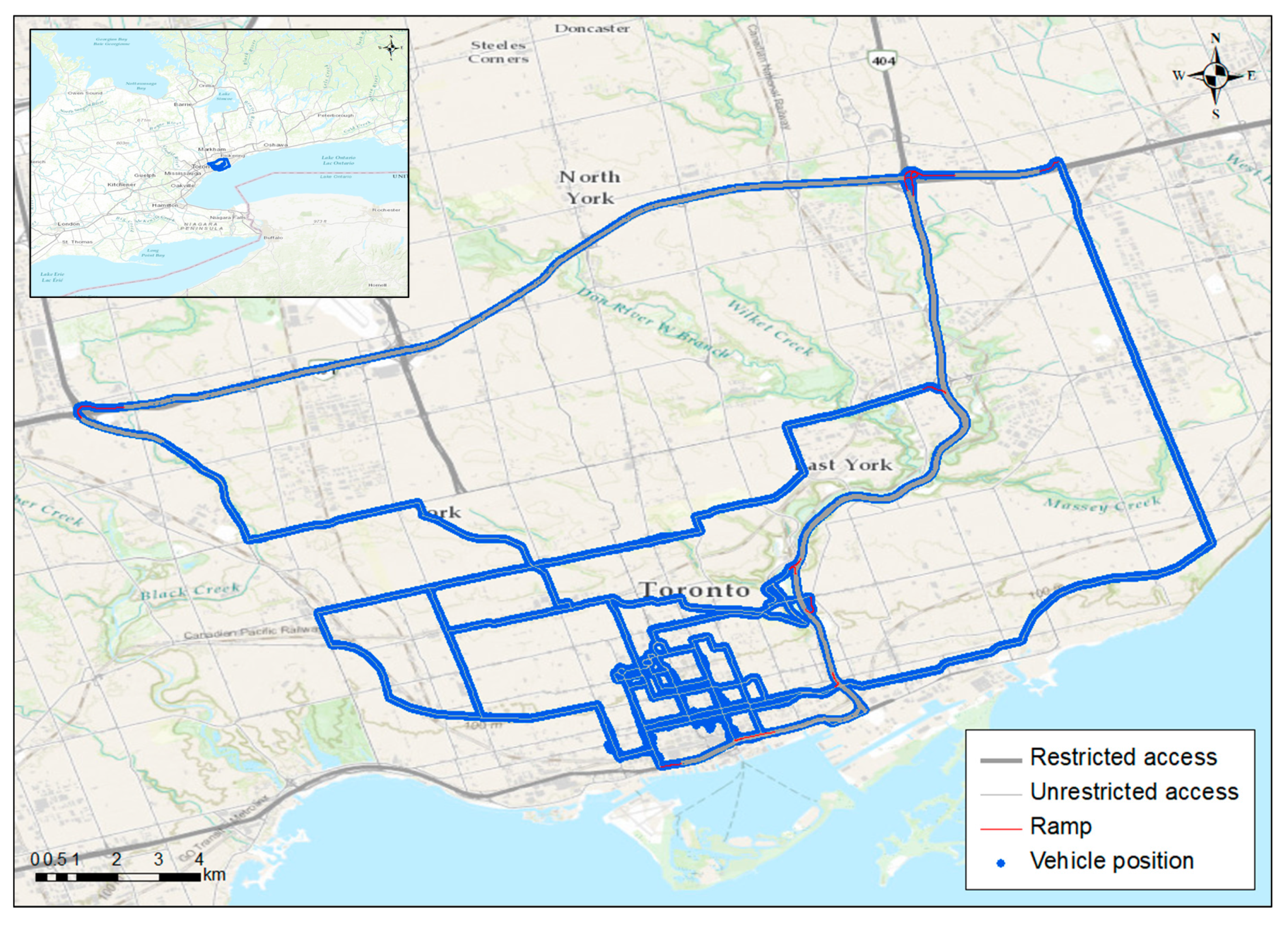
In this study, 31 on-road emission tests were conducted in the City of Toronto between 22 October and 12 December 2019. A 2020 Nissan Rogue SV was tested, and its specifications are listed in Table 2. The tested vehicle used regular gasoline (Octane No. 87) with Sulphur content below 14 mg/kg [28]. The emission measurements were conducted using a SEMTECH DS+ light duty PEMS manufactured by Sensors Inc.: Ann Arbor, USA. The mass emissions of CO2, CO, NOx, and PN were recorded every second during the tests, while HC were not measured, because of the limitations in carrying hydrogen gas in light duty passenger vehicles (HC analysis entails the use of a flame ionization detector). A GPS tracker was installed in the vehicle to record its trajectory. The on-board diagnostics (OBD) data of the vehicle were also collected to monitor the vehicle’s operating parameters. A weather station was installed on the rooftop of the vehicle to record temperature and humidity. In summary, 196,413 data points of CO2, CO, NOx, and PN emissions, timestamp, latitude, longitude, altitude, vehicle speed, acceleration, engine speed, engine torque, engine load, air-fuel ratio, catalyst temperature, and ambient temperature were collected. The vehicle speed ranged from 0 to 121.9 km/h and the ambient temperature ranged from −7 to 37 °C.
Figure 1 illustrates the vehicle trajectory during the tests. The digital map of the road network for the City of Toronto and a map-matching algorithm were employed to match each vehicle position to its corresponding road segment to obtain the road grade and road type, which are available in the map’s database. In this study, the test routes cover all the road types according to the Transportation Association of Canada (TAC) Manual of Geometric Design Standards for Canadian Roads [29], as listed in Table 3.
2.2. Estimates of Emission Variability
For each second, the VSP, which is defined as the instantaneous power per unit mass of the vehicle, was calculated. The instantaneous power generated by the engine is used to overcome the rolling resistance (FRolling) and aerodynamic drag (FAerodynamic), and to increase the kinetic (KE) and potential (PE) energies of the vehicle, as shown in Equation (1) [1].
where m is the vehicle mass, v is the vehicle speed.
In the US EPA modal emissions model MOVES [12], the equation is simplified, and the VSP is calculated based on the vehicle’s speed, acceleration, and road grade, as shown in Equation (2).
where VSP is in kW/t, v is the vehicle’s instantaneous speed in m/s, a is the acceleration in m/s2. A, B, and C are coefficients in kW·s/m, kW·s2/m2, and kW·s3/m3, respectively. A is associated with tire rolling resistance, B with mechanical rotating friction as well as higher order rolling resistance losses, and C with aerodynamic drag. m is the mass for the specific vehicle type in metric ton, g is the acceleration due to gravity, and sin θ is the road grade.
If the vehicle speed is zero (or idling), the VSP is zero; the VSP is negative when the vehicle is decelerating; and if the vehicle is accelerating, the VSP is positive.
In this study, after calculating the VSP associated with each second, a VSP binning method, which is defined by an equal VSP interval of 1 kW/ton, was employed for the purpose of reducing aggregation errors and computational complexity. The coefficient of variation (CV) of CO2, CO, NOx, and PN emissions was calculated to capture the variability in emissions per second along road segments, VSP bins, and across various categories of engine speed, torque, load, air-fuel ratio, vehicle speed, acceleration, altitude, road grade, road type, catalyst temperature, ambient temperature, and time of day. The CV is defined as the ratio of the standard deviation to the mean. The emissions with CV < 1 are considered low-variance, while those with CV > 1 are considered high-variance.
3. Results
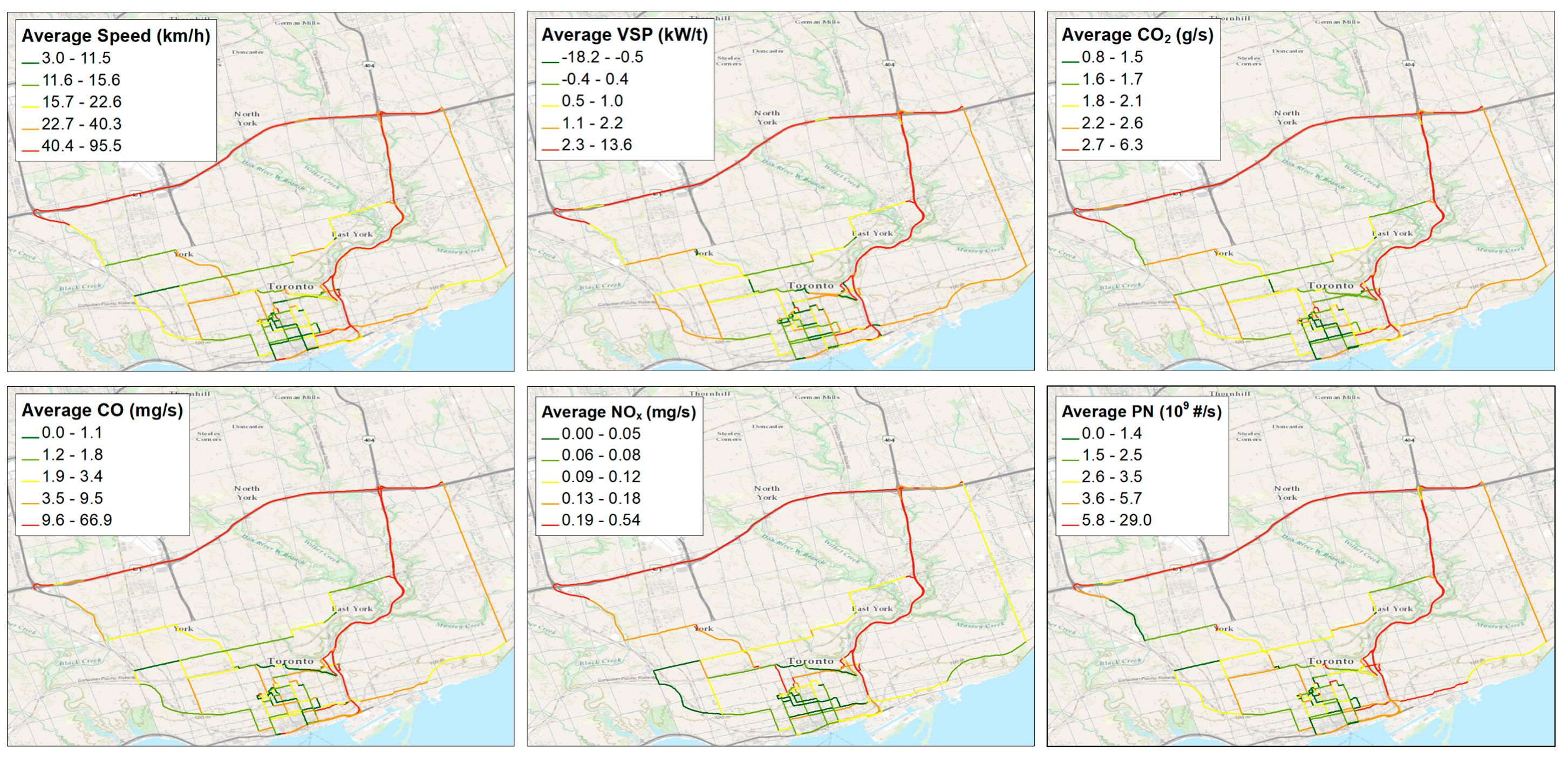
3.1. Average Speed, VSP, and Emissions
The average speed, VSP, CO2, CO, NOx, and PN emissions per second across 156 road segments are illustrated in Figure 2. Each color represents 20% of all the road segments. The average CO2, CO, NOx, and PN emissions show high consistency with the average speed and VSP. This is one of the reasons why the operational emission models employ the average speed and VSP to estimate emissions. We also observe that the average speed, VSP, and emissions for restricted access roads (expressways) are higher than those for unrestricted access roads. In general, the average VSP for expressways was found to be positive and high (between 2.3 and 13.6 kW/t); the VSP for arterial roads was positive and low (between 0.5 and 2.2 kW/t); the VSP for collectors and local streets was negative, which means the vehicle is traveling at low speeds and frequently decelerating. Emissions of CO2 vary in a relatively small range (between 0.82 and 6.35 g/s) and the highest value is 7.4 times the lowest value. CO, NOx, and PN emissions vary in a much larger range: CO emissions are between 0.005 and 219.56 mg/s and the highest/lowest ratio is 43,912; NOx emissions are between 0.001 and 0.539 mg/s and the highest/lowest ratio is 539; PN emissions are between 0.006 and 28.959 × 10⁹ #/s (“#” refers to the number of particles) and the highest/lowest ratio is 4826.5. For the unrestricted access roads, CO and NOx emissions tend to behave in opposite ways. For the road segments with high CO, the NOx is low and vice versa. One of the possible reasons is that the air-fuel ratio has the opposite effects on CO and NOx emissions (during the lean burn, CO is low while NOx is high; and during the rich burn, it is the opposite). This point is further illustrated in Section 3.3.
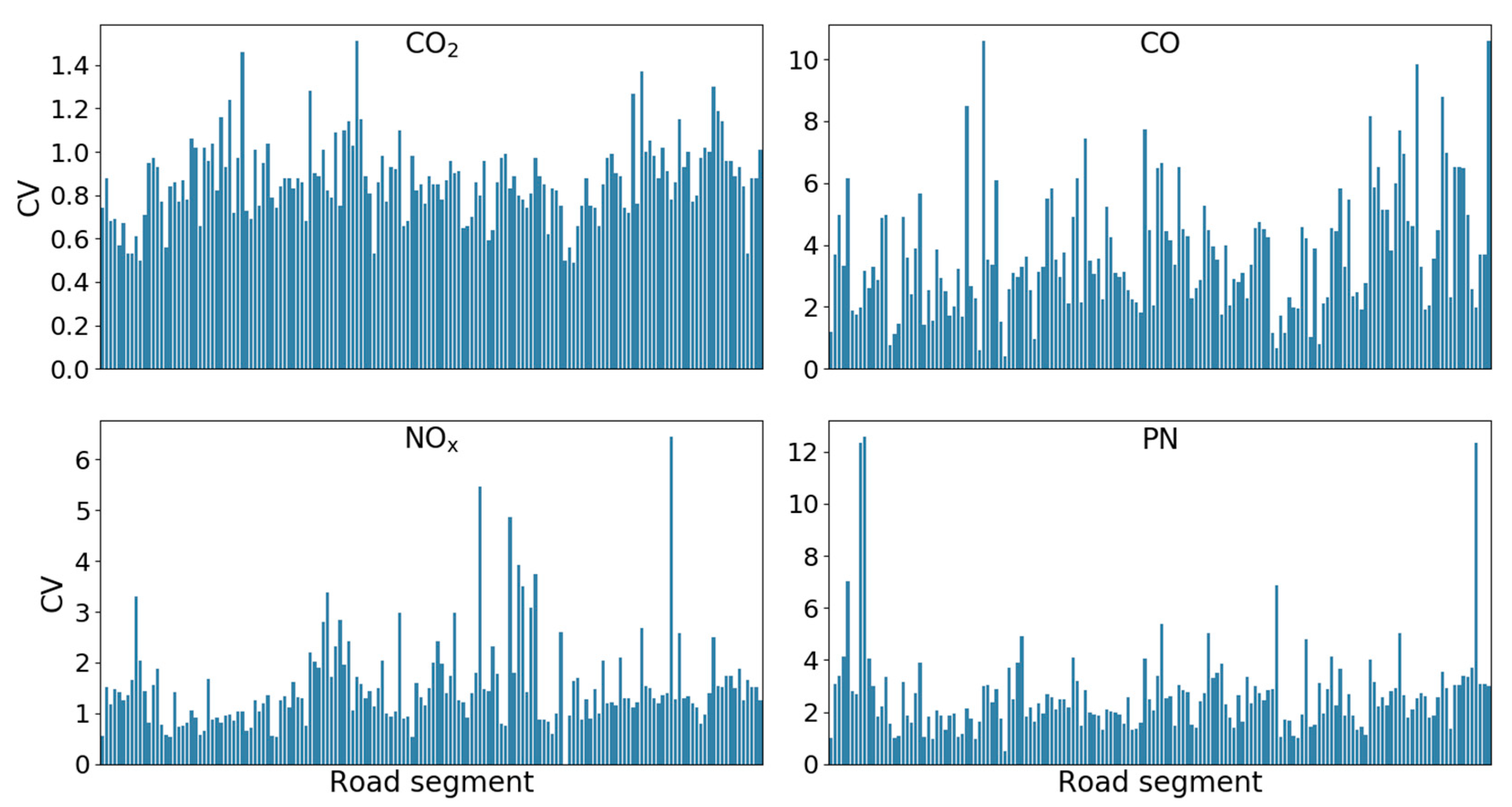
Figure 3 illustrates the CV of emissions on each of the 156 road segments along the test routes, based on the second-by-second measurements conducted during all of the tests which fall on each road segment. Since the vehicle was operating in different modes on each road segment, the CV of CO2, CO, NOx, and PN are high, reaching 1.4, 10, 6, and 12, respectively. The emission variability for some of the road segments is significantly higher, and the variability tends to be higher for the unrestricted access roads, because of stop-and-go driving conditions. The CV of CO, NOx, and PN are particularly higher than the CV of CO2. This is associated with the fact that CO, NOx, and PN emissions not only depend on driving conditions, but also are easily affected by external factors, such as catalyst temperature and ambient temperature on the emission control process.
3.2. Emission Variability in VSP Bins
Figure 4 illustrates the CO2, CO, NOx, and PN emissions in the VSP bins, defined by an equal VSP interval of 1 kW/t. The boxplot captures second-by-second emissions and the bar chart represents the CV. Outliers, which are outside the interquartile range—1.5 times above the upper quartile and below the lower quartile—are not illustrated in the boxplots, and not included in the calculation of CV.
For the tested vehicle, the VSP varies in a range of (−73, 72) kW/t. Over 99.5% of the VSP is in the range of (−30, 30) kW/t. The average emissions of the negative and zero VSP are significantly lower than those of the positive VSP.
CO2 average emissions remain at a very low level in the negative and zero VSP bins, while increasing approximately linearly in the positive VSP bins. CO, NOx, and PN are not monotonically increasing in the positive VSP bins. CO is particularly sensitive to the high positive VSP.
Compared with the variability for the road segments, the variability in each 1 kW/t VSP bin is smaller. However, the CV of emissions is still high, even in the same VSP bin. The CV of CO2 is approximately 0.6, depending on the VSP bins. The CV of CO, NOx, and PN is much higher, and is over 1.0 in most of the VSP bins.
3.3. Emission Variability and Influencing Factors
As discussed in Section 3.2, the emissions in the negative and zero VSP bins remain at a very low level, while the emissions in the positive VSP bins tend to vary depending on the VSP. In this section, the negative VSP bins are merged and the positive VSP are categorized in intervals of 10 kW/t, for the purpose of providing a robust sample size for the analysis of each influencing factor.
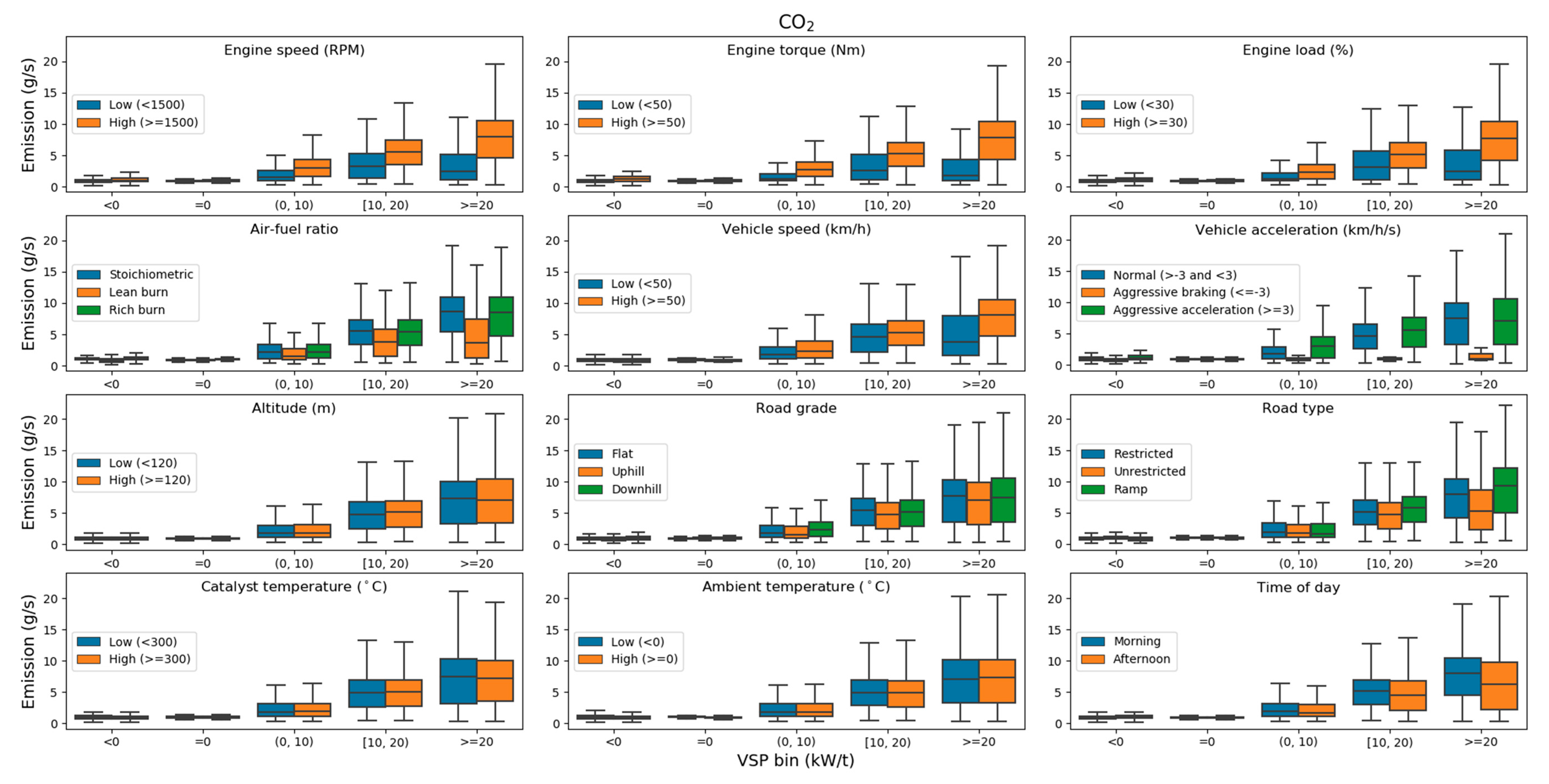
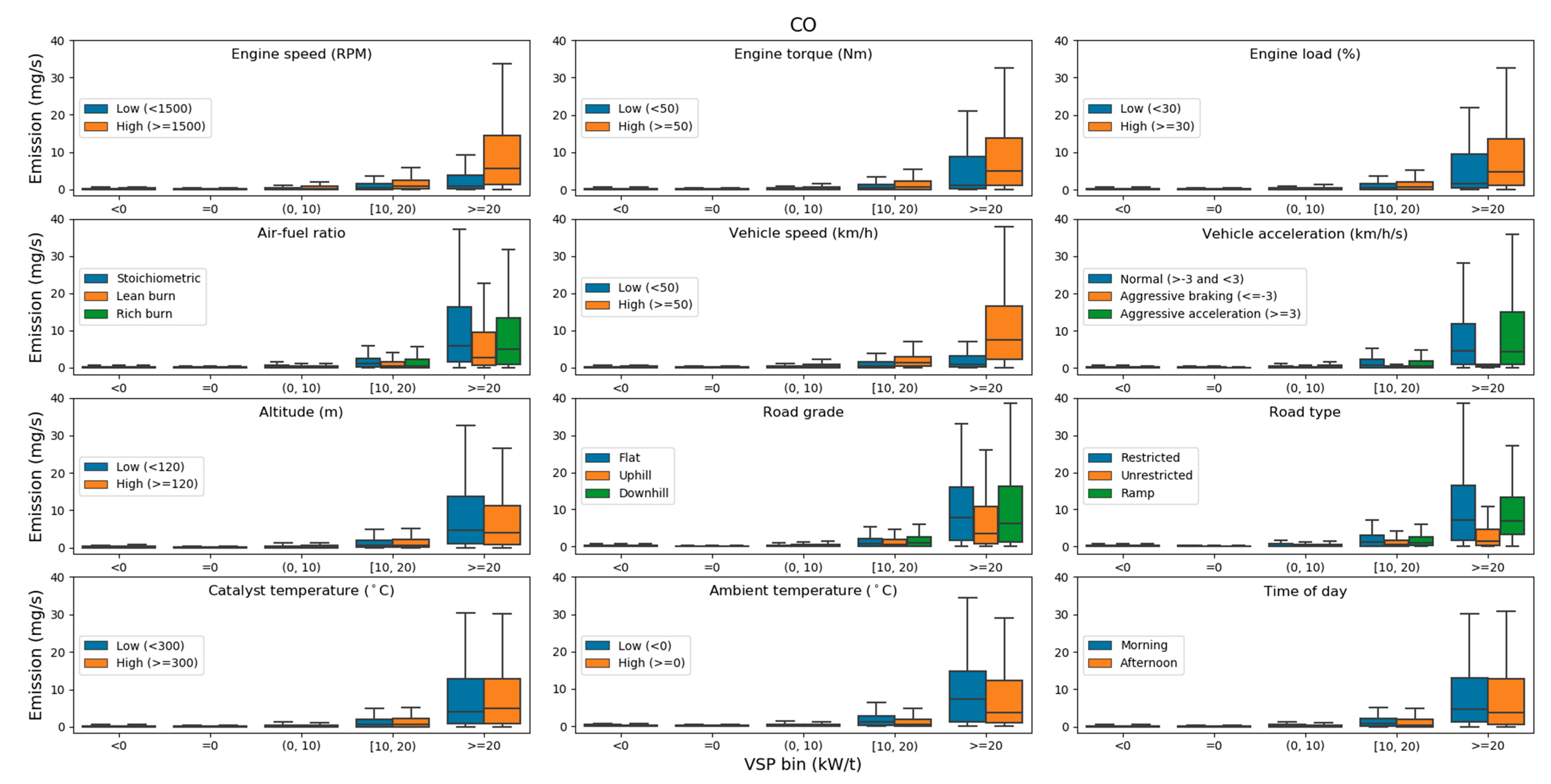
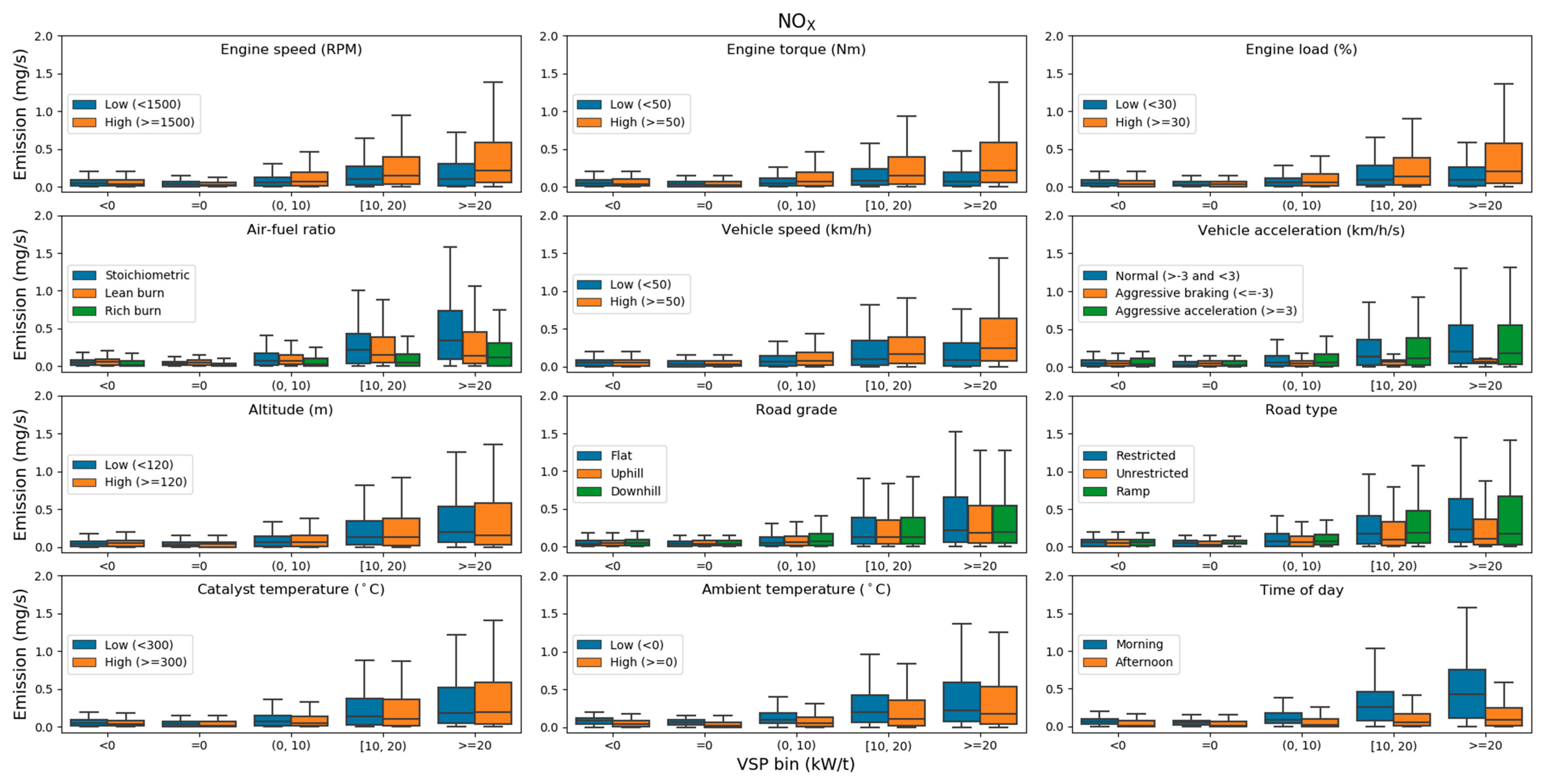
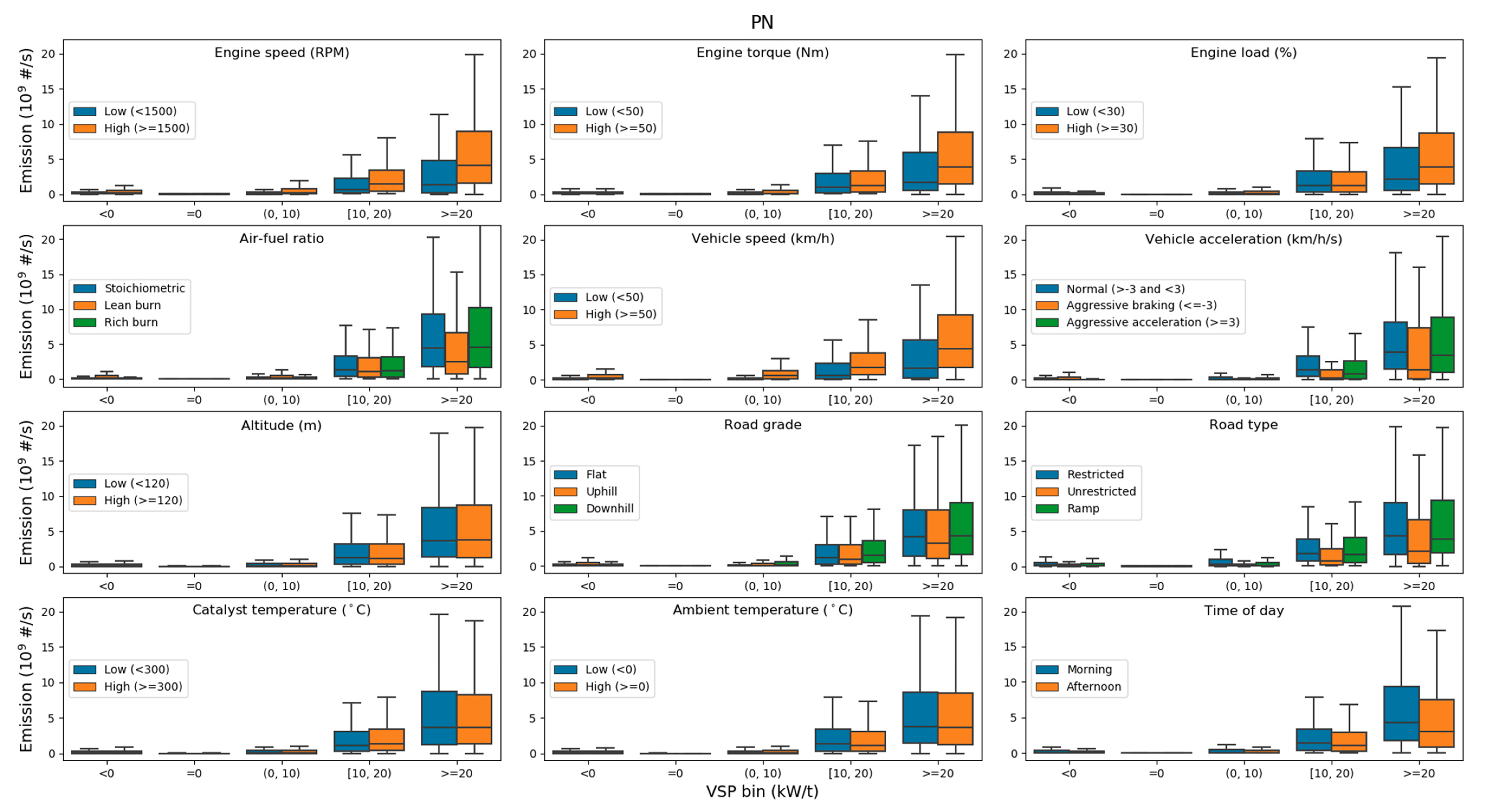
Figure 5, Figure 6, Figure 7 and Figure 8 illustrate the CO2, CO, NOx, and PN emissions per second in each VSP bin across engine speed, torque, load, air-fuel ratio, vehicle speed, acceleration, altitude, road grade, road type, catalyst temperature, ambient temperature, and time of day.
We observe that CO2, CO, NOx, and PN emissions are strongly correlated with engine speed, torque and load. High engine speed, torque, and load produce high emissions. CO2, CO, and PN emissions during lean-burn are significantly lower than the emissions during the stoichiometric mix and rich burn while the NOx emissions during rich burn are the lowest.
Emissions are also strongly associated with vehicle speed and acceleration. The process of high speed and aggressive acceleration produces high emissions while the process of aggressive braking produces low emissions. It should be noted that emissions vary in a very wide range, especially at high engine speed, torque, load, high vehicle speed, and aggressive acceleration.
Previous studies have identified that altitude is one of the dominant factors influencing the CO and NOx emissions in hilly areas [16,17,18]. The City of Toronto is relatively flat, and the maximum altitude difference in the dataset is only approximately 300 m. Thus, the emission differences due to altitude in this study are not significant.
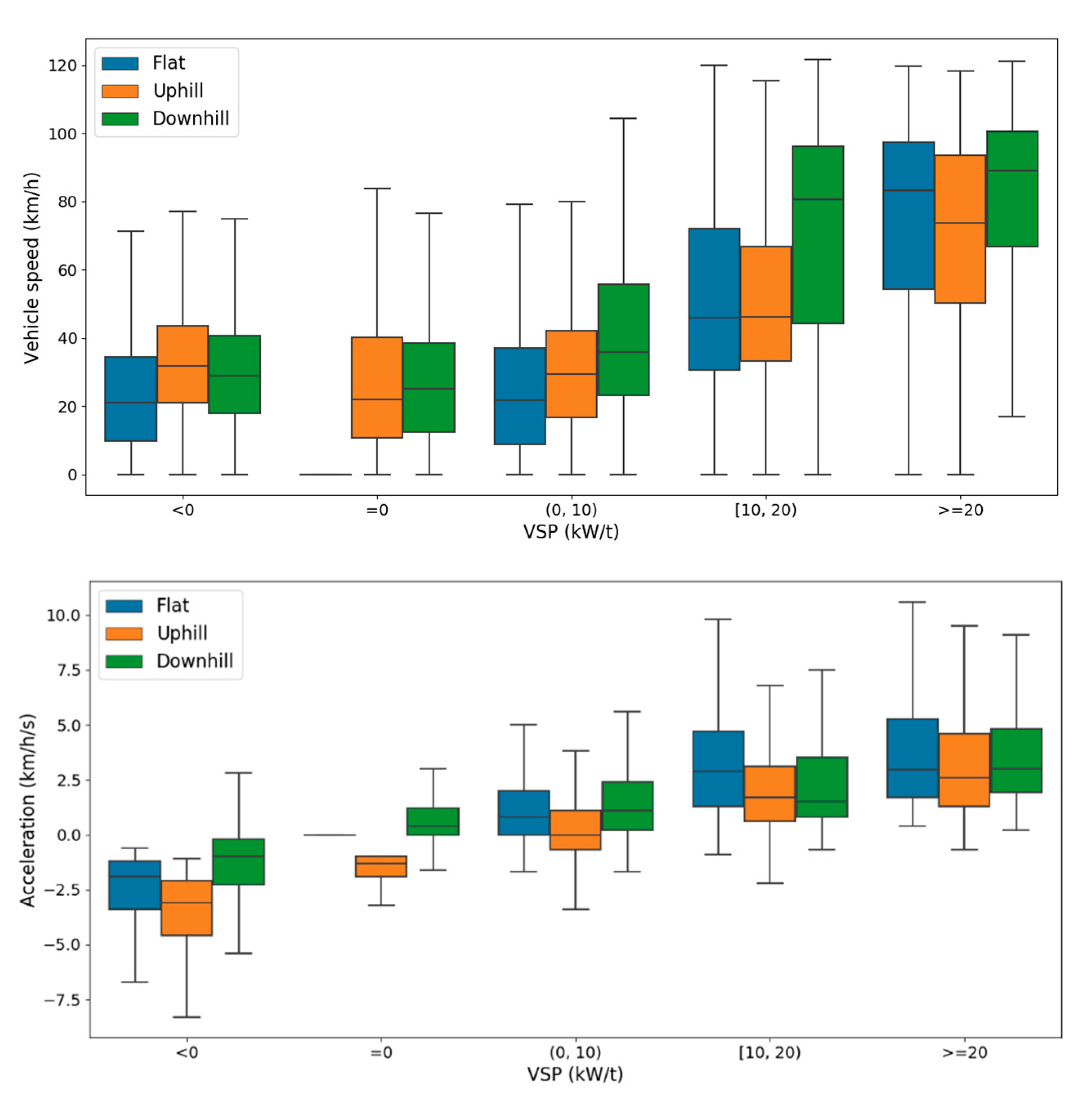
Various studies have investigated the emissions for different road grades and road types on the basis of vehicle speed and acceleration. When comparing the emissions per second on the basis of VSP, the results are different. We observe that in the VSP bins of (0, 10), [10, 20), and >=20 kW/t, the emissions while traveling downhill tend to be higher than the emissions while traveling uphill. In fact, we noted that the vehicle is traveling faster and accelerating more frequently when driving downhill. On average, the vehicle speeds while traveling downhill are 56.7%, 50.3%, and 26.7% higher than the speeds while traveling uphill in the VSP bins of (0, 10), [10, 20), and >=20 kW/t, respectively, and the accelerations while traveling downhill are 298.0%, 11.0%, and 13.1% higher than the acceleration while traveling uphill, as illustrated in Figure 9.
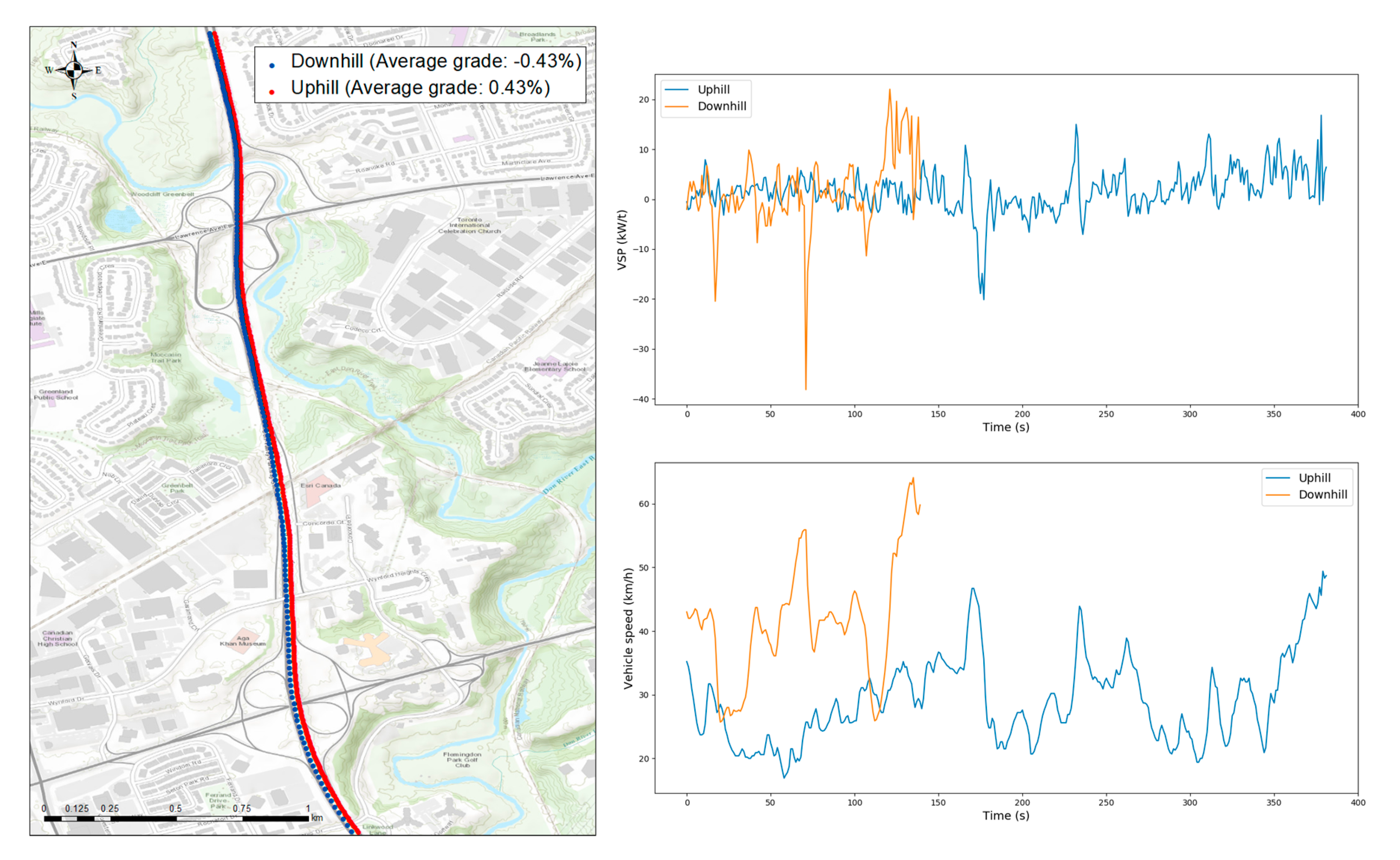
To further explain the effects of road grade, we provide two pieces of data extracted from the emission test results for a stretch of road extending along the Don Valley Parkway, as illustrated in Figure 10. On this specific drive, the vehicle is traveling uphill in Case #1 (average road grade = 0.43%), while it is running downhill in Case #2 (average road grade = −0.43%). The vehicle is traveling at an average VSP of 1.51 kW/t uphill and 1.65 kW/t downhill. In addition, the vehicle speed and acceleration downhill are both higher than under uphill driving (the average speeds uphill and downhill are 29.0 km/h and 41.5 km/h and the average accelerations are 0.037 km/h/s and 0.111 km/h/s, respectively). Consequently, the emissions during downhill driving are also higher.
The emissions for restricted access roads (mainly highways) and ramps are higher than the emissions for unrestricted access roads (like arterial roads with signalized intersections). In fact, the observed vehicle speeds for restricted access roads are approximately twice the speeds for unrestricted access roads while the speeds for ramps are approximately one and a half times the speeds for unrestricted access roads in the VSP bins of (0, 10), [10, 20), and >=20 kW/t. It is not easy to compare the emissions for the restricted access roads and the emissions for the ramps here, because both the emissions for the on-ramp and off-ramp are included.
CO2 emissions are not sensitive to catalyst temperature, ambient temperature, and time of day because: (1) these factors primarily have effects on the emission control process, where the existing CO2 would not be affected, unlike CO, NOx, and HC; and (2) although parts of CO and HC are oxidized to CO2, which causes a very small increase in CO2 emissions, this increase is not substantial, because the existing CO2 is not at the same magnitude as CO and HC emissions (CO2 is in g/s while CO and HC are in mg/s).
For CO, NOx, and PN emissions, the effects of catalyst temperature are not significant. One of the reasons is that in this study, the tested vehicle was picked up from an underground parking lot in the morning (overnight parking is not allowed in the lab) and driven to the lab (about 10 min) for vehicle instrumentation and PEMS calibration prior to the first test route. At noon, the vehicle was parked inside the lab until the afternoon test started. Thus, technically, cold starts were not captured as part of the testing and for each test, the catalyst temperature had reached its efficient range. CO, NOx, and PN emissions at low ambient temperature tend to be higher, because of the poor mixing of fuel and air and the reduced combustion efficiency and stability [27]. The trend for the time of the day is consistent with that for ambient temperature that the emissions in the morning are higher than the emissions in the afternoon, because of the lower ambient temperature in the morning.
4. Conclusions and Recommendations
In this paper, the emissions of a gasoline direct injection vehicle were tested using a state of the art PEMS unit, along two study routes that cover various types of roads and traffic conditions. The paper focuses on documenting the variability in emissions under similar vehicle powers, thus, capturing the effects of other factors affecting emissions. By capturing the variability in emissions occurring at the same VSP, this study sheds light on existing emission models that use the VSP as the main parameter to generate a single deterministic emission estimate. The results will inform the development of future, more robust models, which account for this variability, and promote the development of a binning process that can reduce variability.
Vehicle emissions are strongly associated with engine speed, torque, and load, as well as air-fuel ratio. The process of high engine speed, torque, and load produces high emissions. The CO2, CO, and PN emissions during lean-burn are significantly lower than the emissions during the stoichiometric mix and rich burn, while the NOx emissions during rich burn are the lowest.
Emissions are also strongly associated with vehicle speed and acceleration. The process of high speed and aggressive acceleration produces high emissions, while the process of braking produces low emissions.
We observed that in the same VSP bin, the emissions per second while the vehicle is traveling downhill tend to be higher than the emissions going uphill, because the vehicle is traveling faster and accelerating more frequently when in downhill conditions. Even at the same power, we observed that the vehicle tended to travel faster and accelerated more frequently downhill. The emissions for restricted access roads (highways) and ramps are higher than the emissions for unrestricted access roads (arterial roads), because of the higher speeds.
CO, NOx, and PN emissions at a low ambient temperature tend to be higher. The emissions in the morning are observed to be higher than the emissions in the afternoon, because of the lower ambient temperature.
Author Contributions
Conceptualization, Z.Z. and M.H.; methodology, Z.Z.; software, Z.Z.; validation, Z.Z. and M.H.; formal analysis, Z.Z.; investigation, Z.Z.; resources, M.H.; data curation, Z.Z., R.T., J.X. and A.W.; writing—original draft preparation, Z.Z.; writing—review and editing, Z.Z. and M.H.; visualization, Z.Z.; supervision, M.H.; project administration, M.H.; funding acquisition, M.H. All authors have read and agreed to the published version of the manuscript.
Funding
This research was supported by a grant from the Natural Sciences and Engineering Research Council of Canada RGPAS 493151-16.
Conflicts of Interest
The authors declare no conflict of interest.
References
- Jiménez-Palacios, J.L. Understanding and Quantifying Motor Vehicle Emissions with Vehicle Specific Power and TILDAS Remote Sensing; University of Cambridge: Cambridge, UK, 1999. [Google Scholar]
- Scora, G.; Barth, M. Comprehensive Modal Emission Model (CMEM), version 3.01; User’s Guide; Centre for Environmental Research and Technology, University of California: Riverside, CA, USA, 2006. [Google Scholar]
- Cappiello, A.; Chabini, I.; Nam, E.K.; Lue, A.; Abou Zeid, M. A statistical model of vehicle emissions and fuel consumption. In Proceedings of the IEEE 5th International Conference on Intelligent Transportation Systems, Singapore, 6 September 2002; pp. 801–809. [Google Scholar]
- Sturm, P.J.; Hausberger, S. Emissions and Fuel Consumption from Heavy Duty Vehicles; European Cooperation in Science and Technology: Brussels, Belgium, 2005. [Google Scholar]
- Carolien, B.; Luc, I.; Rudi, T.; Davy, J.; Steven, B. The Application of the Simulation Software Vetess To Evaluate. In Proceedings of the 10th International Conference on Computers in Urban Planning and Urban Management, Iguassu, Brazil, 11–13 July 2007. [Google Scholar]
- US EPA. User’s Guide to MOBILE6.1 and MOBILE6.2: Mobile Source Emission Factor Model; US EPA: Washington, DC, USA, 2002.
- US CARB. EMFAC2007 Version 2.30 Calculating Emission Inventories for Vehicles in California User’s Guide; US CARB: Sacramento, CA, USA, 2006. [Google Scholar]
- Ntziachristos, L.; Gkatzoflias, D.; Kouridis, C.; Samaras, Z. COPERT: A European Road Transport Emission Inventory Model. In Information Technologies in Environmental Engineering; Springer: Berlin/Heidelberg, Germany, 2009; ISBN 978-3-540-88350-0. [Google Scholar]
- US EPA. IVE Model Users Manual Version 2.0; US EPA: Washington, DC, USA, 2008.
- Haan, P.; Keller, M. Emission Factors for Passenger Cars and Light-Duty Vehicles: Handbook Emission Factors for Road Transport (HBEFA), Version 2.1. 2004. Available online: https://www.hbefa.net/e/index.html (accessed on 25 May 2020).
- Rakha, H.; Ahn, K.; Trani, A. Development of VT-Micro model for estimating hot stabilized light duty vehicle and truck emissions. Transp. Res. Part D Transp. Environ. 2004, 9, 49–74. [Google Scholar] [CrossRef]
- US EPA. Population and Activity of On-Road Vehicles in MOVES2014; US EPA: Washington, DC, USA, 2016.
- Abo-Qudais, S.; Qdais, H.A. Performance evaluation of vehicles emissions prediction models. Clean Technol. Environ. Policy 2005, 7, 279–284. [Google Scholar] [CrossRef]
- US EPA. Development of Emission Rates for Light-Duty Vehicles in the Motor Vehicle Emissions Simulator (MOVES2010); US EPA: Washington, DC, USA, 2011.
- Bishop, J.D.K.; Stettler, M.E.J.; Molden, N.; Boies, A.M. Engine maps of fuel use and emissions from transient driving cycles. Appl. Energy 2016, 183, 202–217. [Google Scholar] [CrossRef] [Green Version]
- Boroujeni, B.Y.; Frey, H.C. Road grade quantification based on global positioning system data obtained from real-world vehicle fuel use and emissions measurements. Atmos. Environ. 2014, 85, 179–186. [Google Scholar] [CrossRef]
- Hu, J.; Frey, H.C. Comparison of Real World Light-Duty Gasoline Vehicle Emissions for High Altitude Mountainous Versus Low Altitude Piedmont Study Areas. In Proceedings of the 100th Annual Conference and Exhibition, Air & Waste Management Association, Pittsburgh, PA, USA, 26–29 June 2007. [Google Scholar]
- Nagpure, A.S.; Gurjar, B.R.; Kumar, P. Impact of altitude on emission rates of ozone precursors from gasoline-driven light-duty commercial vehicles. Atmos. Environ. 2011, 45, 1413–1417. [Google Scholar] [CrossRef] [Green Version]
- Wyatt, D.W.; Li, H.; Tate, J.E. The impact of road grade on carbon dioxide (CO2) emission of a passenger vehicle in real-world driving. Transp. Res. Part D Transp. Environ. 2014, 32, 160–170. [Google Scholar] [CrossRef] [Green Version]
- Gallus, J.; Kirchner, U.; Vogt, R.; Benter, T. Impact of driving style and road grade on gaseous exhaust emissions of passenger vehicles measured by a Portable Emission Measurement System (PEMS). Transp. Res. Part D Transp. Environ. 2017, 52, 215–226. [Google Scholar] [CrossRef]
- Costagliola, M.A.; Costabile, M.; Prati, M.V. Impact of road grade on real driving emissions from two Euro 5 diesel vehicles. Appl. Energy 2018, 231, 586–593. [Google Scholar] [CrossRef]
- Varella, R.A.; Faria, M.V.; Mendoza-Villafuerte, P.; Baptista, P.C.; Sousa, L.; Duarte, G.O. Assessing the influence of boundary conditions, driving behavior and data analysis methods on real driving CO2 and NOx emissions. Sci. Total Environ. 2019, 658, 879–894. [Google Scholar] [CrossRef]
- Boriboonsomsin, K.; Barth, M. Impacts of road grade on fuel consumption and carbon dioxide emissions evidenced by use of advanced navigation systems. Transp. Res. Rec. 2009, 2139, 21–30. [Google Scholar] [CrossRef]
- Sentoff, K.M.; Aultman-Hall, L.; Holmén, B.A. Implications of Driving Style and Road Grade for Accurate Vehicle Activity Data and Emissions Estimates. Transp. Res. Part D Transp. Environ. 2015, 35, 175–188. [Google Scholar] [CrossRef]
- De Vlieger, I.; De Keukeleere, D.; Kretzschmar, J. Environmental effects of driving behaviour and congestion related to passenger cars. Atmos. Environ. 2000, 34, 4649–4655. [Google Scholar] [CrossRef]
- Jackson, E.; Qu, Y.; Holmén, B.; Aultman-Hall, L. Driver and Road Type Effects on Light-Duty Gas and Particulate Emissions. Transp. Res. Rec. J. Transp. Res. Board 2006, 1987, 118–127. [Google Scholar] [CrossRef]
- Ko, J.; Jin, D.; Jang, W.; Myung, C.L.; Kwon, S.; Park, S. Comparative investigation of NOx emission characteristics from a Euro 6-compliant diesel passenger car over the NEDC and WLTC at various ambient temperatures. Appl. Energy 2017, 187, 652–662. [Google Scholar] [CrossRef]
- Government of Canada. Sulphur in Gasoline Regulations. Available online: https://www.canada.ca/en/environment-climate-change/services/managing-pollution/energy-production/fuel-regulations/sulphur-gasoline.html (accessed on 1 July 2020).
- Transportation Association of Canada. Geometric Design Guide for Canadian Roads; Transportation Association of Canada: Ottawa, ON, Canada, 2017. [Google Scholar]
Figure 1.
Vehicle emission test routes.

Figure 2.
Average speed, vehicle specific power (VSP), CO2, carbon monoxide (CO), nitrogen oxides (NOx), and particle number (PN) emissions per second for each road segment (“#” refers to the number of particles).
Figure 2.
Average speed, vehicle specific power (VSP), CO2, carbon monoxide (CO), nitrogen oxides (NOx), and particle number (PN) emissions per second for each road segment (“#” refers to the number of particles).

Figure 3.
Coefficient of variation (CV) of emissions for each road segment.

Figure 4.
CO2, CO, NOx, and PN emissions as a function of vehicle specific power.

Figure 5.
CO2 emissions in each VSP bin under various influencing factors.

Figure 6.
CO emissions in each VSP bin under various influencing factors.

Figure 7.
NOx emissions in each VSP bin under various influencing factors.

Figure 8.
PN emissions in each VSP bin under various influencing factors.

Figure 9.
Vehicle speed, acceleration, and VSP while traveling uphill and downhill: (top) vehicle speed distribution and (bottom) distribution of accelerations.
Figure 9.
Vehicle speed, acceleration, and VSP while traveling uphill and downhill: (top) vehicle speed distribution and (bottom) distribution of accelerations.

Figure 10.
Examples of (left) vehicle trajectories uphill and downhill (top right) variation of VSP with time and (bottom right) variation of speed with time.
Figure 10.
Examples of (left) vehicle trajectories uphill and downhill (top right) variation of VSP with time and (bottom right) variation of speed with time.


Table 1.
Existing Emission Models Based on Engine Operation and Vehicle Activity Data.
| Parameter | Model Name | Abbreviation | Reference |
|---|---|---|---|
| Engine Operation | Comprehensive Modal Emission Model | CMEM | [2] |
| Emissions from Traffic | EMIT | [3] | |
| Passenger Car and Heavy-Duty Emission Model | PHEM | [4] | |
| Vehicle Transient Emissions Simulation Software | VeTESS | [5] | |
| Vehicle activity | Mobile Source Emission Factor Model | MOBILE | [6] |
| Emission Factors Model | EMFAC | [7] | |
| Computer Program to Calculate Emissions from Road Transport | COPERT | [8] | |
| International Vehicle Emission Model | IVE | [9] | |
| Handbook Emission Factors for Road Transport | HBEFA | [10] | |
| Virginia Tech Microscopic Model | VT-Micro | [11] | |
| Motor Vehicle Emissions Simulator | MOVES | [12] |
Table 2.
Specifications of Tested Vehicle.
| Specifications | Value |
|---|---|
| Engine | 2.5-Litre DOHC 16-Valve 4-Cylinder |
| Horsepower | 170 HP @ 6,000 RPM |
| Torque | 175 lb-ft @ 4,400 RPM |
| Curb weight | 1,681 kg |
| Mileage | 500 km |
| Fuel type | Regular Gasoline |
| Fuel injection type | GDI |
| Emission standard | Tier 2, Bin 5 |
| Transmission | Automatic |
| Turbo-compound | No |
| Ignition type | Direct ignition system |
Table 3.
Road Types and Length of Road Segments along Test Routes.
| Road Type for Emission Model | Road Type | Length (km) |
|---|---|---|
| Restricted access | Expressway | 28.9 |
| Ramp | Expressway ramp | 7.2 |
| Unrestricted access | Major arterial | 70.4 |
| Minor arterial | 20.9 | |
| Collector | 2.9 | |
| Local | 1.3 | |
| Other | 1.3 | |
| Total | 132.8 | |
© 2020 by the authors. Licensee MDPI, Basel, Switzerland. This article is an open access article distributed under the terms and conditions of the Creative Commons Attribution (CC BY) license (http://creativecommons.org/licenses/by/4.0/).
Share and Cite
MDPI and ACS Style
Zhai, Z.; Tu, R.; Xu, J.; Wang, A.; Hatzopoulou, M. Capturing the Variability in Instantaneous Vehicle Emissions Based on Field Test Data. Atmosphere 2020, 11, 765. https://doi.org/10.3390/atmos11070765
AMA Style
Zhai Z, Tu R, Xu J, Wang A, Hatzopoulou M. Capturing the Variability in Instantaneous Vehicle Emissions Based on Field Test Data. Atmosphere. 2020; 11(7):765. https://doi.org/10.3390/atmos11070765
Chicago/Turabian StyleZhai, Zhiqiang, Ran Tu, Junshi Xu, An Wang, and Marianne Hatzopoulou. 2020. "Capturing the Variability in Instantaneous Vehicle Emissions Based on Field Test Data" Atmosphere 11, no. 7: 765. https://doi.org/10.3390/atmos11070765
Note that from the first issue of 2016, this journal uses article numbers instead of page numbers. See further details here.