


1 Introduction
Generally, one would like to be able to model the self-consistent low-frequency dynamics (below the gyrofrequency) of plasma in general time-varying electromagnetic fields. In order for a gyrokinetic approach to be feasible, certain constraints on the amplitude or wavelength of the fields are implied, but these should ideally be as weak as possible. We have derived a gyrokinetic formalism, in a Lagrangian formalism, which allows for quite general fields (McMillan & Sharma Reference McMillan and Sharma2016): this paper is motivated by questions of how to derive and implement equations of motion in such theories. Essentially, the complication relative to more standard gyrokinetic theories is that the self-consistent electromagnetic fields appear in the symplectic part of the Lagrangian. Although certain other formalisms share this feature (a review of the typical theory is found in Brizard & Hahm (Reference Brizard and Hahm2007)), additional issues arise due to the more general nature of the symplectic scheme in McMillan & Sharma (Reference McMillan and Sharma2016), as well as in certain drift kinetic theories (Miyato et al. Reference Miyato, Scott, Strintzi and Tokuda2009) and higher-order weak-flow gyrokinetics (Parra & Catto Reference Parra and Catto2008): time derivatives of the field appear both in the equations of motion and the field equation, unlike in the standard symplectic electromagnetic (EM) formulation. These additional terms in the field equation, under investigation here, are formally small, and thus tempting to treat as corrections, unlike the terms that appear in the standard symplectic EM formulation.
Some somewhat subtle problems then arise in the specification and solution of such equations, and their relationship to standard gyrokinetic theory (Burby Reference Burby2016); the ‘auxiliary field’  $\unicode[STIX]{x1D719}$ appears as a dynamical variable requiring an initial condition, and unphysical rapid variation of the solutions to the Euler–Lagrange equations appears. This is odd because the field
  $\unicode[STIX]{x1D719}$ may be written in terms of the particle distribution function in Vlasov–Maxwell theory, so should not appear as an extra degree of dynamical freedom. Burby (Reference Burby2016) explains a method to resolve this; we will explain a related approach to removing these unphysical degrees of freedom, as well as how to implement a more direct approach that simply imposes regular behaviour in the small-perturbation limit. We will first explain how these complications arise in an electrostatic theory (Sharma & McMillan Reference Sharma and McMillan2015).
The normalised gyrocentre particle Lagrangian up to first order in this formalism is
 $$\begin{eqnarray}\displaystyle L_{\text{p}} & = & \displaystyle [\boldsymbol{A}(\boldsymbol{R})+v_{\Vert }\hat{\boldsymbol{b}}+\boldsymbol{u}]\boldsymbol{\cdot }\dot{\boldsymbol{R}}+\unicode[STIX]{x1D707}\dot{\unicode[STIX]{x1D703}}\nonumber\\ \displaystyle & & \displaystyle -\,({\textstyle \frac{1}{2}}v_{\Vert }^{2}+\unicode[STIX]{x1D707}B+{\textstyle \frac{1}{2}}\boldsymbol{u}^{2}+\langle \unicode[STIX]{x1D719}\rangle ),\end{eqnarray}$$
 where  $\boldsymbol{A}$ is the magnetic vector potential,
  $\boldsymbol{R}$ is the gyrocentre position,
  $v_{\Vert }$ is the parallel particle velocity,
  $\hat{\boldsymbol{b}}$ is the magnetic field unit vector,
  $\unicode[STIX]{x1D707}$ is the magnetic moment,
  $\unicode[STIX]{x1D703}$ is the gyroangle,
  $B$ is the magnetic field strength,
 $$\begin{eqnarray}\langle \unicode[STIX]{x1D713}\rangle (\boldsymbol{R},\unicode[STIX]{x1D707},t)=\frac{1}{2\unicode[STIX]{x03C0}}\int \text{d}\unicode[STIX]{x1D703}\,\text{d}^{3}r\unicode[STIX]{x1D6FF}(\boldsymbol{R}+\unicode[STIX]{x1D746}-\boldsymbol{r})\unicode[STIX]{x1D713}(\boldsymbol{r},t)\end{eqnarray}$$
 defines the gyroaveraging operator,  $\unicode[STIX]{x1D746}$ is the gyroradius vector,
  $\boldsymbol{r}$ is the field position,
  $\unicode[STIX]{x1D719}(\boldsymbol{r},t)$ is the electrostatic potential,
 $$\begin{eqnarray}\boldsymbol{u}=\boldsymbol{b}\times \unicode[STIX]{x1D735}\langle \unicode[STIX]{x1D719}\rangle /B\end{eqnarray}$$
 is the flow velocity and  $t$ is time. Note that this formalism is equivalent to standard symplectic electrostatic drift-kinetic theory if the gyroaveraging is suppressed, and the drift-kinetic Euler–Lagrange equations are subject to the same complication.
For simplicity, we consider two-dimensional simulations in the plane perpendicular to the magnetic field. For this geometry, we can find equations of motion and a field equation obtained from our first-order gyrocentre Lagrangian from variational theory. The equations of motion are
 $$\begin{eqnarray}\left.\begin{array}{@{}c@{}}\dot{\boldsymbol{R}}=\boldsymbol{u}+v_{\Vert }\hat{\boldsymbol{b}}+B_{\Vert }^{\ast -1}\hat{\boldsymbol{b}}\times \dot{\boldsymbol{u}}_{1},\\ \dot{v}_{\Vert }=0\quad \text{and}\\ \dot{\unicode[STIX]{x1D707}}=0.\end{array}\right\}\end{eqnarray}$$
Note that, unlike standard gyrokinetic theory, the polarisation drift now appears in the drift motion, in terms of the time derivative of the flow (note that the polarisation drift appears in the equations of motion even in certain weak-flow formalisms (Heikkinen et al. Reference Heikkinen, Janhunen, Kiviniemi and Ogando2008)).
The field equation is
 $$\begin{eqnarray}0=\int \text{d}^{6}Z\unicode[STIX]{x1D6FF}(\boldsymbol{R}+\unicode[STIX]{x1D746}-\boldsymbol{r})(B_{\Vert }^{\ast }F+B^{-1}\unicode[STIX]{x1D735}\boldsymbol{\cdot }[F\dot{\boldsymbol{u}}_{1}]),\end{eqnarray}$$
 where  $F$ is the gyrocentre distribution function and
  $\text{d}^{6}Z=B_{\Vert }^{\ast }\,\text{d}\boldsymbol{R}\,\text{d}v_{\Vert }\,\text{d}\unicode[STIX]{x1D707}\,\text{d}\unicode[STIX]{x1D703}$. We have
 $$\begin{eqnarray}B_{\Vert }^{\ast }=\hat{\boldsymbol{b}}\boldsymbol{\cdot }(\boldsymbol{B}+\unicode[STIX]{x1D735}\times \boldsymbol{u})=B+B^{-1}\unicode[STIX]{x1D6FB}^{2}\langle \unicode[STIX]{x1D719}\rangle\end{eqnarray}$$
and
 $$\begin{eqnarray}\dot{\boldsymbol{u}}_{1}=(\unicode[STIX]{x2202}_{t}+\boldsymbol{u}\boldsymbol{\cdot }\unicode[STIX]{x1D735})\boldsymbol{u}.\end{eqnarray}$$
The first term in the field equation (1.5) contains the effect of polarisation through the dependence of the phase-space volume on potential (as the polarisation drift is retained in the gyrocentre trajectory). These equations reduce to drift-kinetic theory if the gyroaverage is set to an identity.
The third term in the equation for  $\dot{\boldsymbol{R}}$ (in (1.4)) and the second term in the right-hand parentheses in our Poisson equation (1.5) contain a partial time derivative of the potential-dependent flow velocity. These terms, however, are actually of higher order (in
  $\unicode[STIX]{x1D716}=\unicode[STIX]{x1D6FB}^{2}\unicode[STIX]{x1D719}$) than the dominant terms in these expressions: this is obvious for the polarisation drift, but it requires some work to show why the term in the Poisson equation is small (and the distribution function must not have too strong a gradient). We would therefore be justified in neglecting them, given the theory is only valid up to first order. It is nonetheless useful to keep them, in order to derive a conservative numerical scheme: we are interested in solving over transport time scales where secular accumulation of small fluxes might potentially be important. Retaining these formally small terms is also necessary for consistency if higher-order terms are kept in the Lagrangian.
A difficulty arises because both the field equation and the equation of motion involve the polarisation drift (as in Heikkinen et al. (Reference Heikkinen, Janhunen, Kiviniemi and Ogando2008)), so involve the time derivative of the electrostatic potential. We will show why for these equations, an iterative solution approach is justified. Essentially, this is permitted by the formal smallness of the time derivatives, so they may be treated as corrections; if they were large, on the other hand, they would fundamentally change the nature of the equations.
In certain other symplectic electromagnetic formalisms (indeed, in the formalism often just called symplectic gyrokinetics), the field time-derivative term (of the parallel vector potential) in the equations of motion is of the same order as the remaining perturbed motion and, in particular, contains the lowest-order physics of the Alfvén waves. Thus, a direct iterative approach would not normally converge (Belli & Hammett Reference Belli and Hammett2005); however, where the time derivative of the fields only appears in the equations of motion and not the field equation, an explicit equation for the time derivative of  $A_{\Vert }$ may be written by taking the time derivative of the field equation and substituting in the Vlasov equation (Manuilskiy & Lee Reference Manuilskiy and Lee2000; Görler et al. Reference Görler, Lapillonne, Brunner, Dannert, Jenko, Merz and Told2011; Mandell et al. Reference Mandell, Hakim, Hammett and Francisquez2020). That is, these terms do not actually lead to the conceptual and numerical problems explored in this paper. In a general setting, a combination of that approach and the iterative scheme described in this paper may be necessary: an explicit equation for the lowest-order solution of the time dependence of the fields, plus an iteration approach to deal with small terms that create a dependence on higher-order time derivatives.
2 Converting between symplectic and Hamiltonian forms
One approach to solving systems with a symplectic form containing a time-varying field is to split the symplectic form into a large part and a correction,  $\unicode[STIX]{x1D6FE}_{i}=\unicode[STIX]{x1D6FE}_{i}^{0}+\unicode[STIX]{x1D716}\unicode[STIX]{x1D6FE}_{i}^{1}$, where
  $\unicode[STIX]{x1D6FE}_{i}^{0}(Z,t)$ is independent of the perturbed field, and find a change of variables to convert to a Hamiltonian approach. The choice of splitting is obvious for perturbative theories. Another approach is to use a splitting based on an approximate solution
  $\unicode[STIX]{x1D719}^{0}$ for the fields, which is dependent on the particle positions, but not on
  ${\dot{Z}}$ (a related version of this approach is suggested in Burby (Reference Burby2016)). One may then write
  $\unicode[STIX]{x1D6FE}(\unicode[STIX]{x1D719},Z)=\unicode[STIX]{x1D6FE}(\unicode[STIX]{x1D719}^{0},Z)+\unicode[STIX]{x1D6FE}(\unicode[STIX]{x1D719}-\unicode[STIX]{x1D719}^{0})$: in our case,
  $\unicode[STIX]{x1D719}^{0}$ is found by neglecting the second term in the Poisson equation. We then identify
  $\unicode[STIX]{x1D6FE}^{0}=\unicode[STIX]{x1D6FE}(\unicode[STIX]{x1D719}^{0},Z)$ and
  $\unicode[STIX]{x1D6FE}^{1}=\unicode[STIX]{x1D6FE}(\unicode[STIX]{x1D719}-\unicode[STIX]{x1D719}^{0})$.
In order to keep the splitting procedure entirely described within the variational formalism, an additional equation describing the approximate Poisson equation, and thus  $\unicode[STIX]{x1D719}^{1}$, may be added to the system Lagrangian via a Lagrange multiplier. Neither the splitting nor this additional equation modify the solutions to the dynamical equations, but simply serve to identify a small term
  $\unicode[STIX]{x1D6FE}_{1}$ in the symplectic form. The particle Lagrangian
  $L$ may then be transformed to show that
 $$\begin{eqnarray}\displaystyle L & = & \displaystyle (\unicode[STIX]{x1D6FE}_{i}^{0}+\unicode[STIX]{x1D716}\unicode[STIX]{x1D6FE}_{i}^{1})\,\text{d}Z_{i}+(\unicode[STIX]{x1D6FE}_{0}^{0}+\unicode[STIX]{x1D716}\unicode[STIX]{x1D6FE}_{0}^{1})\,\text{d}t\nonumber\\ \displaystyle & = & \displaystyle \unicode[STIX]{x1D6FE}_{i}^{0}\,\text{d}Z_{i}^{\prime }+ [\unicode[STIX]{x1D6FE}_{0}^{0}+\unicode[STIX]{x1D716}\,\text{d}S/\text{d}t+\unicode[STIX]{x1D716}\unicode[STIX]{x1D6FE}_{0}^{1}\nonumber\\ \displaystyle & & \displaystyle +\,\unicode[STIX]{x1D716}(\unicode[STIX]{x1D6FE}_{i}^{1}-\text{d}S/\text{d}Z_{i})\unicode[STIX]{x1D714}_{ij}^{-1}\unicode[STIX]{x1D714}_{j0} ]\,\text{d}t+O(\unicode[STIX]{x1D716}^{2}),\end{eqnarray}$$
 where a near-unity transform  $Z^{\prime }=T(Z)$ has been used to eliminate
  $\unicode[STIX]{x1D6FE}^{1}$ from the symplectic form,
  $\unicode[STIX]{x1D714}$ is the Poisson matrix associated with
  $\unicode[STIX]{x1D6FE}^{0}$,
  $S$ is a gauge function that may be chosen to simplify the Hamiltonian, the implied sums are over indices
  $i\in 1,6$ and all functions in the last line are evaluated at
  $Z^{\prime }$. The Lie transform approach may be used to eliminate
  $\unicode[STIX]{x1D6FE}^{1}$ from the symplectic form at all orders, but only the solution at lowest order is shown explicitly.
For standard symplectic EM theories, the transform  $T$ amounts to the replacement
  $p_{\Vert }=qA_{\Vert }+mv_{\Vert }$. Taking instead
  $p_{\Vert }=q(A_{\Vert }-A_{\Vert }^{0})+mv_{\Vert }$, where
  $A_{\Vert }^{0}$ is an approximate solution for the vector potential (for example, one may compute its time dependence using the zero-resistivity limit of Ohm’s law
  $E_{\Vert }=0$) is the basis for the partially symplectic approach of Mishchenko et al. (Reference Mishchenko, Bottino, Hatzky, Sonnendrücker, Kleiber and Könies2017). The transform performed in this section is a generalisation of the partially symplectic approach for general Lagrangian forms. As a result of the transform, the perturbed field now appears only in the Hamiltonian, through
  $\unicode[STIX]{x1D6FE}_{1}$. Variation of the potential then results in a field equation dependent only on the set of particle coordinates
  $Z$, but not on
  ${\dot{Z}}$ (in the standard symplectic EM case, the result is the integral of the
  $p_{\Vert }$ current). The result is a solution for
  $\unicode[STIX]{x1D719}$ and thus
  $\dot{Z^{\prime }}$ consistent with the original Lagrangian, which may locally (in a short time window) be expressed as a power-series expansion in
  $\unicode[STIX]{x1D716}$.
We do not pursue this approach as a practical way to solve gyrokinetic equations: the use of an approximate field solution as part of an additional transform appears likely to lead to particularly messy expressions for general cases. But this approach does show the existence of a solution (for the particle trajectories  $\boldsymbol{Z}$ and
  $\unicode[STIX]{x1D719}$) which has a regular power-series expansion, as long as an approximate solution
  $\boldsymbol{A}^{0}$ may be found. We will use a more direct approach to find the terms in the expansion order-by-order.
3 Form of the field equation in this symplectic theory
In general, gyrokinetic theory is an asymptotic theory, constructed on the assumption that the local dynamics (i.e. over a sufficiently short time interval), and thus  $\unicode[STIX]{x1D719}$ and
  $Z$, depend smoothly on a small parameter, so they may be written (over short time intervals) as an asymptotic power-series expansion in terms of the ordering parameter
  $\unicode[STIX]{x1D716}$ and time. That is, the formalism neglects effects which are asymptotically small, such as resonances between gyration and drift motion, because they do not appear in the power-series expansion, as well as effects on short time scales comparable to the gyration time. Note that the correct ordering of generators in the Lie transform also depends on the smooth dependence of the dynamics, which is a requirement to be able to derive gyrokinetic theories using Lie transform methods. The considerations of the previous section demonstrate that we may convert the symplectic formalism to a Hamiltonian formulation where there is no time derivative of the field in the Poisson equation, and solve it in the usual way, to find a solution regular as
  $\unicode[STIX]{x1D716}\rightarrow 0$. It is more straightforward however to simply determine the terms in this power series directly without an additional coordinate transform.
Time derivatives appear in the Poisson equation, equation (1.5), multiplied by (some power of) the ordering parameter with a dependence of the form
 $$\begin{eqnarray}0=\unicode[STIX]{x1D716}A\frac{\text{d}\unicode[STIX]{x1D719}}{\text{d}t}+B\unicode[STIX]{x1D719}+C.\end{eqnarray}$$
 A direct solution of this equation coupled to the particle equations of motion requires an initial condition for  $\unicode[STIX]{x1D719}$, which is surprising, since in a low-frequency (Darwin) theory we expect
  $\unicode[STIX]{x1D719}$ to be a function of the particle positions. Also, if we were to ignore the required slow time variation of the solutions, the derivative term would be a singular perturbation, because the ordering parameter multiplies the highest-order term. Solutions in general would vary in a singular fashion as
  $\unicode[STIX]{x1D716}\rightarrow 0$, rather than smoothly approaching the
  $\unicode[STIX]{x1D716}=0$ limit. The typical variation time scale would go as
  $\unicode[STIX]{x1D716}^{-1}$ as
  $\unicode[STIX]{x1D716}\rightarrow 0$, which is not formally compatible with the assumed time-scale ordering of gyrokinetics. In order to impose that the term multiplied by
  $\unicode[STIX]{x1D716}$ be small, we find a power-series expansion in
  $\unicode[STIX]{x1D716}$ that satisfies the equation.
Singular initial-value differential equations may often be solved by separating space into a transient (inner) region with rapid time variation where the term involving high-order time derivatives is comparable to other terms, and a smooth outer region, where the singular term is relatively small (O’Malley Jr. Reference O’Malley2013). The outer solution is defined as the limit of a Picard iteration (and this is generally how it is found in practice). That is, given  $\unicode[STIX]{x1D719}_{0}$ satisfying
  $B\unicode[STIX]{x1D719}_{0}+C=0$ and, for
  $n>0$,
 $$\begin{eqnarray}0=\unicode[STIX]{x1D716}A\frac{\text{d}\unicode[STIX]{x1D719}_{n}}{\text{d}t}+B\unicode[STIX]{x1D719}_{n+1}+C\end{eqnarray}$$
 and the outer solution is taken to be  $\unicode[STIX]{x1D719}=\lim _{n\rightarrow \infty }\unicode[STIX]{x1D719}_{n}$. These equations need to be solved simultaneously with the Vlasov equation (or equations of motion in the Lagrangian formulation), which also involves the derivative of the field
  $\unicode[STIX]{x1D719}$ and determines the operators
  $A,B$ and
  $C$ (most obviously because the particle distribution determines the gyrocentre charge density); we have
 $$\begin{eqnarray}\frac{\text{d}\boldsymbol{Z}_{n+1}}{\text{d}t}=\dot{\boldsymbol{Z}}^{0}(\unicode[STIX]{x1D719}_{n+1})+\unicode[STIX]{x1D716}\dot{\boldsymbol{Z}}^{1}\left(\frac{\text{d}\unicode[STIX]{x1D719}_{n}}{\text{d}t}\right),\end{eqnarray}$$
 where  $Z^{0}$ and
  $Z^{1}$ denote the equations of motion (1.4) split by order of the terms. If this process converges,
  $\unicode[STIX]{x1D719}$ is a solution to the original equation, with a smooth dependence on
  $\unicode[STIX]{x1D716}$ near
  $\unicode[STIX]{x1D716}=0$. We do not attempt to find conditions under which this series converges; proving this would require an examination of the spectral properties of the problem-specific operators. For well-behaved systems, one expects a finite radius of convergence in
  $\unicode[STIX]{x1D716}$ (because the iteration involves a small parameter, unlike Belli & Hammett (Reference Belli and Hammett2005)).
Given that the fast dynamics appears to be spurious, and that the physical dynamics, at least locally, should smoothly tend to the  $\unicode[STIX]{x1D716}=0$ case in the
  $\unicode[STIX]{x1D716}\rightarrow 0$ limit, we suggest that this outer solution is the physically relevant one. Because this choice also removes the extra degrees of freedom (specification of the initial value of
  $\unicode[STIX]{x1D719}$), this allows an unambiguous specification of the initial conditions using the particle distribution. The outer solution then satisfies both the initial condition and the time-evolution equations (gyroVlasov–Maxwell), and evolves on time scales consistent with the assumed time-scale ordering, and thus meets the requirements of a correct solution. There may well be physical transient dynamics that occurs on faster time scales (comparable to the gyrofrequency), but we have, in any case, chosen to neglect this as part of the gyrokinetic ordering, so it is consistent to also neglect it here.
4 Numerical solution of outer time-evolution equations
The outer solution to the time-evolution equations is defined using a Picard iteration method, and numerical methods can directly implement this iteration procedure. As part of this process, the time derivative of the field must be evaluated and, given the value of the field on the time-grid points, this may be constructed using standard finite-difference methods. Numerical methods to solve these asymptotic methods are not novel (Abrahamsson, Keller & Kreiss Reference Abrahamsson, Keller and Kreiss1974; O’Malley Jr. Reference O’Malley2013), but will likely be unfamiliar to most plasma physicists.
We will illustrate how such methods work by describing a simple approach based on the fourth-order Runge–Kutta integrator. Based on the values at either end of the Runge–Kutta time step, a time-continuous interpolator for the field (a dense representation) may be constructed, to allow the time derivative to be calculated for the next Picard iteration. We represent the equation to be solved as
 $$\begin{eqnarray}U\frac{\text{d}X}{\text{d}t}=A(X)+\unicode[STIX]{x1D716}B\frac{\text{d}X}{\text{d}t}+\unicode[STIX]{x1D716}^{2}C\frac{\text{d}^{2}X}{\text{d}t^{2}},\end{eqnarray}$$
 where  $X$ is some general (e.g. vector) quantity. For the gyrokinetic problem, the variable
  $X$ would represent the extended system state
  $(\unicode[STIX]{x1D719},f)$, and the operators
  $U,A,B$ and
  $C$ encode the coupled Vlasov–Poisson system.
We choose to construct  $X_{0}(t)$ via a standard fourth-order Runge–Kutta scheme, which we take two steps of, from time point
  $T$ to
  $T+h/2$, then to time point
  $T+h$. Five intermediate values
  $X_{i}(T)$,
  $X_{i}^{\prime }(T)$,
  $X_{i}(T+h/2)$,
  $X_{i}^{\prime }(T+h/2)$ and
  $X_{i}(T+h)$ are used, here with
  $i=0$, to construct a fourth-order polynomial interpolant
  $X^{\dagger }(t)$ on the domain
  $t\in [T,T+h]$. Differentiation of
  $X^{\dagger }$ then yields approximations to the first and second derivatives on the domain that are accurate to order
  $h^{4}$ and
  $h^{3}$, respectively.
The Picard iteration procedure then consists of solving
 $$\begin{eqnarray}U\frac{\text{d}X_{i}}{\text{d}t}=A(X_{i})+\unicode[STIX]{x1D716}B\frac{\text{d}X_{i-1}^{\dagger }}{\text{d}t}+\unicode[STIX]{x1D716}^{2}C\frac{\text{d}^{2}X_{i-1}^{\dagger }}{\text{d}t^{2}}\end{eqnarray}$$
 for each  $i$ using Runge–Kutta and then finding the dense approximant
  $X^{\dagger }$ (with
  $X_{-1}=0$). The time derivative has accuracy one order in
  $h$ lower than the Runge–Kutta solution, but is multiplied by
  $\unicode[STIX]{x1D716}$ in the iteration step, so the overall accuracy of the method is
  $\sum _{N=0}^{P}h^{N}\unicode[STIX]{x1D716}^{P-N}$, where
  $P=4$ is the accuracy of the Runge–Kutta scheme we have chosen. Also, the formal accuracy does not improve after the fourth iteration. We illustrate the first two steps of this iteration scheme.
First, we solve the unperturbed system
 $$\begin{eqnarray}U\frac{\text{d}X_{0}}{\text{d}t}=A(X_{0})\end{eqnarray}$$
 and find  $X_{0}^{\dagger }\sim X_{0}$. The next iteration is then constructed using
 $$\begin{eqnarray}U\frac{\text{d}X_{1}}{\text{d}t}=A(X_{1})+\unicode[STIX]{x1D716}B\frac{\text{d}X_{0}^{\dagger }}{\text{d}t}+\unicode[STIX]{x1D716}^{2}C\frac{\text{d}^{2}X_{0}^{\dagger }}{\text{d}t^{2}}\end{eqnarray}$$
 and the order  $\unicode[STIX]{x1D716}$ and
  $\unicode[STIX]{x1D716}^{2}$ terms involving higher-order time derivatives may be directly evaluated to yield a time-varying inhomogeneous term on the right-hand side of the equation; this is a first-order ordinary differential equation for
  $X_{1}$.
Although this provides a method to construct a solution to the order of accuracy desired, the computational expense scales like  $P+1$. A more efficient approach is, apart from at the first time step, to reuse the polynomial interpolant from the previous time step. This is most obviously compatible with the use of multi-step methods where the maximum step size is small compared to Runge–Kutta-type methods, so the amount of extrapolation required is small. If stability is not significantly modified due to finite-
 $\unicode[STIX]{x1D716}$ effects, the computational expense is not significantly worse than the
  $\unicode[STIX]{x1D716}=0$ case.
Note that this approach may also be used as a way of speeding up various iterative schemes found in certain gyrokinetic codes (Mishchenko, Könies & Hatzky Reference Mishchenko, Könies and Hatzky2005; Bottino et al. Reference Bottino, Scott, Brunner, McMillan, Tran, Vernay, Villard, Jolliet, Hatzky and Peeters2010). That is, we can use polynomial extrapolation to find an accurate ‘starting’ value for these schemes.
4.1 Two example problems
Two problems are considered. The first is a first-order nonlinear problem (which tests the nonlinear behaviour of the scheme) and the second is a linear second-order ordinary differential equation with constant coefficients and a forcing (demonstrating that we can find the outer solution to a singular perturbation problem).
First, consider the equation
 $$\begin{eqnarray}{\dot{y}}=\text{e}^{-y}+\unicode[STIX]{x1D716}{\dot{y}},\end{eqnarray}$$
which has the solution
 $$\begin{eqnarray}y=\log \left[\frac{t}{1-\unicode[STIX]{x1D716}}+\text{e}^{y_{0}}\right].\end{eqnarray}$$
 We will solve this problem using the iterative approach discussed in the previous section. To check that the implementation matches the theoretical scaling, we perform a single step of this augmented RK4 scheme and examine the dependence of the error on  $\unicode[STIX]{x1D716}$ and
  $h$. Three scans are performed in the range
  $h=[0.01,0.1]$, with
  $\unicode[STIX]{x1D716}=h^{\unicode[STIX]{x1D6FC}}$ for
  $\unicode[STIX]{x1D6FC}\in \{1/2,1,2\}$. The dominant errors per unit time should scale as
  $O(\unicode[STIX]{x1D716}^{b}h^{4-b})$ with
  $b\in [0,4]$. Therefore, we expect that for
  $\unicode[STIX]{x1D6FC}\in \{1,2\}$ the error should scale as
  $O(h^{4})$ and for
  $\unicode[STIX]{x1D6FC}=1/2$ it should scale as
  $O(h^{2})$; this is confirmed numerically in figure 1.
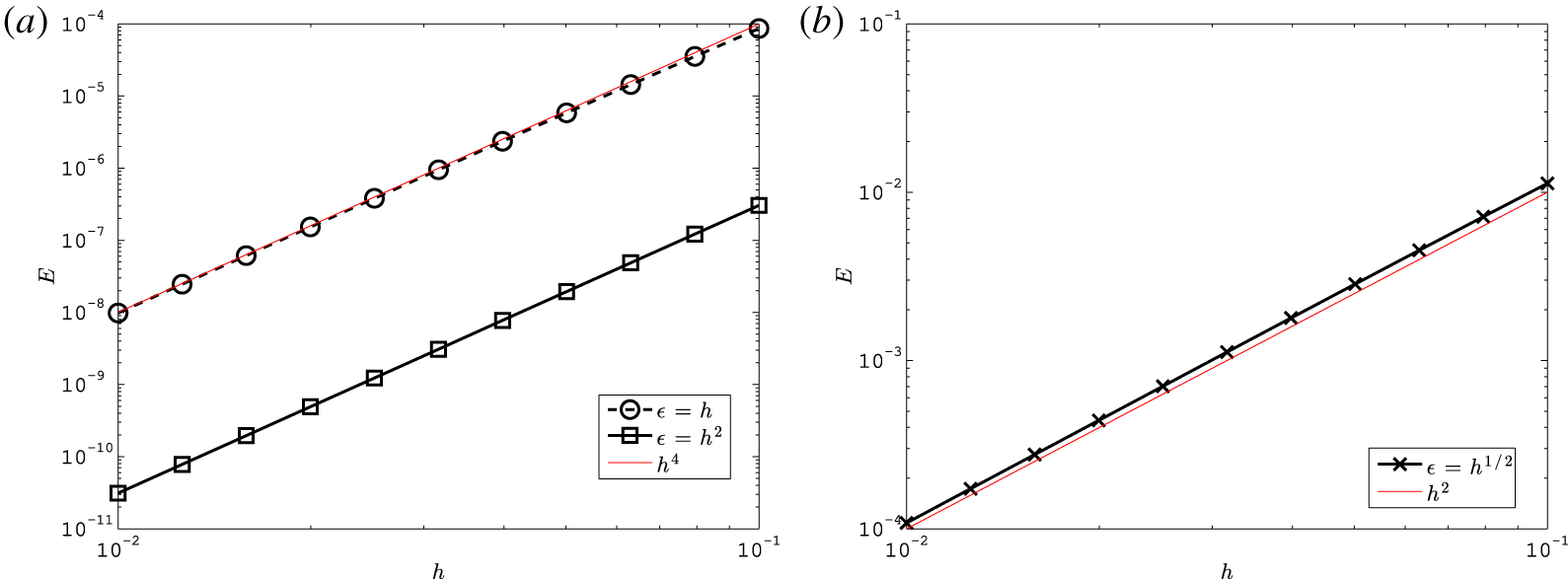
Figure 1. Absolute error per unit time, versus time step  $h$, of the augmented RK4 scheme used to solve (4.5), for (a)
  $\unicode[STIX]{x1D716}=h$ and
  $\unicode[STIX]{x1D716}=h^{2}$, and (b)
  $\unicode[STIX]{x1D716}=h^{1/2}$. These are plotted in black with the expected scaling shown as a red trace.
Second, take the equation
 $$\begin{eqnarray}\unicode[STIX]{x1D716}\frac{\text{d}^{2}y}{\text{d}t^{2}}+\frac{\text{d}y}{\text{d}t}=\cos (t),\end{eqnarray}$$
which has the solution
 $$\begin{eqnarray}y=C_{1}\exp (-t/\unicode[STIX]{x1D716})+C_{2}+\frac{1}{1+\unicode[STIX]{x1D716}^{2}}(\sin (t)-\unicode[STIX]{x1D716}\cos (t)),\end{eqnarray}$$
 where the outer solution with  $C_{1}=0$ does not exhibit the rapid transient. We solve for the outer solution using the same iterative numerical method with
  $\unicode[STIX]{x1D716}=0.1$ and time step
  $h=1/3$. The analytical solution and the error as a function of time are plotted in figure 2. Adequate numerical performance is seen.

Figure 2. Numerical solution to (4.7) (solid trace), and the difference between this and the exact solution (dashed trace), multiplied by  $10^{4}$, for
  $\unicode[STIX]{x1D716}=0.1$ and
  $h=1/3$.
5 Numerical scheme for implicit Vlasov–Poisson
To demonstrate that this methodology may be practically implemented in a gyrokinetic code, we discretise the Vlasov–Poisson equations (equations (1.4) and (1.5)) using a  $\unicode[STIX]{x1D6FF}f$ particle-in-cell (PIC) method (Lanti et al. Reference Lanti, Ohana, Tronko, Hayward-Schneider, Bottino, McMillan, Mishchenko, Scheinberg, Biancalani and Angelino2020) and use the resulting code for two example applications. Monte Carlo markers are used to represent distribution function quanta, employing the splitting
  $F=F_{0}+\unicode[STIX]{x1D6FF}F$, where we choose the equilibrium part
  $F_{0}=n_{0}(2\unicode[STIX]{x03C0}T)^{-3/2}\text{e}^{-((1/2)v_{\Vert }^{2}+\unicode[STIX]{x1D707}B)/T}$ to be Maxwellian,
  $n_{0}(\boldsymbol{R})$ is the background density,
  $T(\boldsymbol{R})$ is the temperature,
  $v$ is the particle velocity and the fluctuating part
  $\unicode[STIX]{x1D6FF}F$ is discretised as follows.
5.1 Discretisation
We define
 $$\begin{eqnarray}\displaystyle \unicode[STIX]{x1D6FF}F & = & \displaystyle N_{\text{p}}N^{-1}\mathop{\sum }_{n=1}^{N}2\unicode[STIX]{x03C0}B_{\Vert }^{\ast -1}w_{n}(t)\unicode[STIX]{x1D6FF}(\boldsymbol{R}-\boldsymbol{R}_{n}(t))\unicode[STIX]{x1D6FF}(\unicode[STIX]{x1D707}-\unicode[STIX]{x1D707}_{n}(t))\nonumber\\ \displaystyle & & \displaystyle \times \,\unicode[STIX]{x1D6FF}(v_{\Vert }-v_{\Vert n}(t)),\end{eqnarray}$$
 where  $N_{\text{p}}$ is the number of particles,
  $N$ is the number of markers and
  $w_{n}$ is the marker weight. Integrating both sides of (5.1) over a region
  $Q$ of volume
  $V_{n}$ associated with a single marker (the marker phase-space volume) and considering the limit where this volume is small, so quantities may be considered constant in this volume, we have
 $$\begin{eqnarray}\unicode[STIX]{x1D6FF}F_{n}V_{n}=N_{\text{p}}N^{-1}w_{n}(t),\end{eqnarray}$$
 where  $\unicode[STIX]{x1D6FF}F_{n}$ is the average value of
  $\unicode[STIX]{x1D6FF}F$ over
  $Q$, with
 $$\begin{eqnarray}V_{n}=\int _{Q}\text{d}^{6}z_{n}\end{eqnarray}$$
 and  $\text{d}^{6}z_{n}=B_{\Vert }^{\ast }\,\text{d}^{3}R\,\text{d}\unicode[STIX]{x1D707}\,\text{d}v_{\Vert }\,\text{d}\unicode[STIX]{x1D703}$. The value of
  $V_{n}$ depends on how the markers are loaded. More specifically, based on the algorithm chosen for sampling phase space, we can compute the distribution of markers
  $g(\boldsymbol{Z})$, which is defined so that over some volume the total number of markers is
 $$\begin{eqnarray}N=\int gB\,\text{d}^{3}R\,\text{d}\unicode[STIX]{x1D707}\,\text{d}v_{\Vert }\,\text{d}\unicode[STIX]{x1D703}.\end{eqnarray}$$
We then have
 $$\begin{eqnarray}V_{n}=B_{\Vert }^{\ast }/gB.\end{eqnarray}$$
 If we load our markers uniformly in some region of  $\boldsymbol{R}$ and
  $(\unicode[STIX]{x1D707},v_{\Vert })$, then we have
  $g$ constant in this region and zero elsewhere. The magnitude of
  $g$ is then the total number of markers divided by the volume of the phase-space region where markers are loaded.
5.2 Initialisation: phase-space volume
Since  $B_{\Vert }^{\ast }$, defined in (1.6), is potential-dependent, we cannot directly find
  $V_{n}$ (5.5) even though
  $g$ is known. Instead, we use the approximation
  $B_{\Vert }^{\ast }=B$ as an initial approximation to
  $V_{n}$. We can then set
  $w_{n}$ from the specified initial distribution using (5.2).
Upon computing the potential to lowest order in  $\unicode[STIX]{x1D716}$, we compute
  $B_{\Vert }^{\ast }$ and then find the corrected value for
  $V_{n}$ (at first order in
  $\unicode[STIX]{x1D716}$). To keep
  $\unicode[STIX]{x1D719}$ constant when correcting
  $V_{n}$, we do not alter
  $w_{n}$. This means that although the state of the initialisation is internally consistent, the actual initial
  $\unicode[STIX]{x1D6FF}F_{n}$ in the simulation is slightly modified compared to the nominal value specified in the input file. Note that higher-order corrections to the potential depend on
  $V_{n}$, so this update would need to be included in the iterative loop at the first time step to allow higher-order consistency: the current implementation does not account for this.
5.3 Time evolving the Vlasov–Poisson system
We have discussed general methods for solving coupled time-evolution equations like our Vlasov–Poisson equations. For our proof-of-principle code, however, we use a simplified low-order method. Our Poisson equation (1.5) and the Euler–Lagrange equation (1.4) contain an implicit term involving  $\dot{\boldsymbol{u}}_{1}$, which cannot be directly computed from the system state (marker weights and positions). We use a single-step method in order to compute
  $\dot{\boldsymbol{u}}_{1}$. We begin by taking a small Euler time step of length
  $h^{\prime }$ with the terms involving
  $\dot{\boldsymbol{u}}_{1}$ neglected. We may then approximate
  $\dot{\boldsymbol{u}}_{1}$ via finite differences as
 $$\begin{eqnarray}\displaystyle \dot{\boldsymbol{u}}_{1}(t) & = & \displaystyle h^{\prime -1} (\boldsymbol{u}\{\boldsymbol{R}(t)+h^{\prime }\boldsymbol{u}[\boldsymbol{R}(t),t],t+h^{\prime }\}\nonumber\\ \displaystyle & & \displaystyle -\,\boldsymbol{u}\{\boldsymbol{R}(t),t\}).\end{eqnarray}$$
 In order to evolve our markers, we use a fourth-order Runge–Kutta time-integration scheme. This requires evaluating the time derivative of the trajectories for each substep, at time points within the interval  $[t,t+h]$. At each substep, an Euler time step of length
  $h^{\prime }$ is used to evaluate the implicit time derivatives, which are correct to first order in
  $\unicode[STIX]{x1D716}$ and
  $h^{\prime }$. Overall, the error per unit time of this method (analysed in the same way as the methods described above) is
  $O(h^{4}+\unicode[STIX]{x1D716}h^{\prime }+\unicode[STIX]{x1D716}^{2})$.
6 Gyrokinetic simulations
6.1 Kelvin–Helmholtz instability
6.1.1 Weak flows
In the weak-flow and cold-ion limits, our Vlasov–Poisson system is equivalent to the Hasegawa–Mima equation (Hasegawa & Mima Reference Hasegawa and Mima1977; Horton & Hasegawa Reference Horton and Hasegawa1994). The Hasegawa–Mima equation exhibits cascade and inverse cascade phenomena, and describes perpendicular modes that lie in the plane perpendicular to a slab magnetic field. Analytic linear growth rates may be computed by assuming a three-wave coupling, for which
 $$\begin{eqnarray}|\unicode[STIX]{x1D719}_{\boldsymbol{k}_{1}}|\gg |\unicode[STIX]{x1D719}_{\boldsymbol{k}_{2}}|\sim |\unicode[STIX]{x1D719}_{\boldsymbol{k}_{3}}|\gg |\unicode[STIX]{x1D719}_{\boldsymbol{k}_{n}}|,\quad n\neq 1,2,3,\end{eqnarray}$$
 where  $\unicode[STIX]{x1D719}_{\boldsymbol{k}_{m}}$ is the complex Fourier mode amplitude,
  $\boldsymbol{k}_{m}$ is a wavevector and
  $n,m\in \mathbb{Z}^{+}$.
Weak-flow code verification was performed by comparing linear Kelvin–Helmholtz instability growth rates computed from gyrokinetic simulations with the analytic and semi-analytic results.
The converged simulations used gyrokinetic hydrogen ions,  $2^{24}$ markers, adiabatic electrons, uniform background densities, uniform ion and electron temperatures, an ion to electron temperature ratio of
  $T_{\text{i}}/T_{\text{e}}=10^{-4}$ and a time step equal to the ion thermal gyroperiod. The doubly periodic, two-dimensional spatial simulation domain used a
  $64\times 32$ grid in (
 $x,y$) and a length
  $\unicode[STIX]{x03C0}\unicode[STIX]{x1D70C}_{\text{ti}}$ in the
  $y$ direction.
The potential was initialised to contain background and perturbation sinusoidal components in the  $y$ and
  $x$ directions, respectively. This was achieved by initialising
  $\unicode[STIX]{x1D6FF}f$ as
 $$\begin{eqnarray}\unicode[STIX]{x1D6FF}f=A[\sin (k_{y}R_{y})+10^{-4}\cos (k_{x}R_{x})]F_{0},\end{eqnarray}$$
 where  $A=47.5$ is the
  $\unicode[STIX]{x1D6FF}f$ amplitude and
  $k_{x}$ and
  $k_{y}=2\unicode[STIX]{x1D70C}_{\text{ti}}^{-1}$ are the wavenumbers in the
  $x$ and
  $y$ directions, respectively (a scan over
  $k_{x}$ was performed at fixed
  $k_{y}$).
As multiple unstable modes are present in the simulation, we do not expect agreement with the analytic, three-wave-coupling result (6.1), but do expect agreement with a semi-analytic result derived in a similar manner to that of Rogers & Dorland (Reference Rogers and Dorland2005) as follows.
During the linear period of the simulation, the potential is given by
 $$\begin{eqnarray}\unicode[STIX]{x1D719}_{\text{a}}=A\sin (k_{y}y)+\text{e}^{\unicode[STIX]{x1D6FE}t+\text{i}k_{x}x}\mathop{\sum }_{n=-\infty }^{\infty }\unicode[STIX]{x1D719}_{n}\text{e}^{\text{i}nk_{y}y},\end{eqnarray}$$
 where  $\unicode[STIX]{x1D6FE}$ is the linear growth rate and
  $i$ in an exponent is the imaginary unit. By substituting this potential (6.3) into the Hasegawa–Mima equation, we obtain the eigenvalue equation
 $$\begin{eqnarray}\displaystyle & & \displaystyle \mathop{\sum }_{n=-\infty }^{\infty }\{\unicode[STIX]{x1D6FE}(n^{2}k_{y}^{2}+k_{x}^{2}+1)+\text{i}Ak_{x}k_{y}[(n^{2}-1)k_{y}^{2}+k_{x}^{2}]\nonumber\\ \displaystyle & & \displaystyle \times \,\cos (k_{y}y)\}\unicode[STIX]{x1D719}_{n}\text{e}^{\text{i}nk_{y}y}=0.\end{eqnarray}$$
By using a change of basis via
 $$\begin{eqnarray}\mathop{\sum }_{n=-\infty }^{\infty }\unicode[STIX]{x1D719}_{n}\text{e}^{\text{i}nk_{y}y}=\mathop{\sum }_{n=0}^{\infty }a_{n}\cos nk_{y}y+\mathop{\sum }_{n=1}^{\infty }b_{n}\sin nk_{y}y\end{eqnarray}$$
and the orthogonality of sine and cosine, the eigenvalue equation (6.4) can be written in the form
 $$\begin{eqnarray}M\boldsymbol{a}=\unicode[STIX]{x1D6FE}\boldsymbol{a},\end{eqnarray}$$
 where  $M\in \mathbb{C}^{n\times n}$ is an infinite square matrix,
  $n\in \mathbb{Z}^{+}$,
  $\boldsymbol{a}=a_{m}$ and
  $m\in \mathbb{Z}^{\ast }$. The eigenvalue equation in this form (6.6) can be solved numerically by computing the maximum real eigenvalues of a truncation of
  $M$ that corresponds to our finite discretised spectral range.
The simulated, semi-analytic (6.6) and analytic (6.1) linear Kelvin–Helmholtz instability growth-rate spectra are shown in figure 3. As expected, we only have good quantitative agreement between the simulated and semi-analytic (6.6) spectra.

Figure 3. Linear Kelvin–Helmholtz instability growth-rate spectra for the gyrokinetic simulation (points) and semi-analytic result (solid curve). The analytic, three-wave-coupling result (dashed curve) is shown for comparison. The simulation parameters are described in § 6.1.1.
6.1.2 Strong flows
The growth rate of the conventional Kelvin–Helmholtz instability is symmetric with respect to the sign of the parallel vorticity. However, for extended magnetohydrodynamics (MHD) that includes finite-Larmor-radius effects (Nagano Reference Nagano1978), an asymmetry appears (this effect has also been seen with hybrid codes (Gingell et al. Reference Gingell, Chapman, Dendy and Brady2012)).
The simulations used gyrokinetic hydrogen ions,  $2^{23}$ markers, constant electron density, uniform background ion density, uniform ion and electron temperatures,
  $T_{\text{i}}=T_{\text{e}}$ and a time step equal to the thermal gyroperiod. The doubly periodic, two-dimensional spatial simulation domain used a
  $64\times 64$ grid in (
 $x,y$) and a length
  $L_{y}=40\unicode[STIX]{x03C0}\unicode[STIX]{x1D70C}_{\text{ti}}$ in the
  $y$ direction. The potential was initialised to contain a shear layer dominated by a single sign of the parallel vorticity with
  $u\sim 1$ in the
  $y$ direction, and a sinusoidal perturbation in the
  $x$ direction. This was achieved by initialising
  $\unicode[STIX]{x1D6FF}f$ as
 $$\begin{eqnarray}\unicode[STIX]{x1D6FF}f=A\{\exp [-{\textstyle \frac{1}{2}}(y-L_{y}/2)^{2}/\unicode[STIX]{x1D70E}^{2}]+c+10^{-4}\cos (k_{x}x)\}F_{0},\end{eqnarray}$$
 where  $A=\pm 2.54\times 10^{-4}$ is the
  $\unicode[STIX]{x1D6FF}f$ amplitude (the sign of which allows the initialisation to be dominated by the corresponding sign of parallel vorticity),
  $\unicode[STIX]{x1D70E}=L_{y}/13.43$,
  $k_{x}$ is the wavenumber in the
  $x$ direction and
  $c=-\sqrt{\unicode[STIX]{x03C0}}/13.43$ is chosen to enforce the requirement that the total charge density in the simulation domain is zero.
The implicit term  $\dot{\boldsymbol{u}}_{1}$ (1.7) is a polarisation drift term that contains the centrifugal drift (Brizard Reference Brizard1995). Without the sinusoidal perturbation in
  $\unicode[STIX]{x1D6FF}f$ (6.7), this initialisation corresponds to a laminar flow, for which
  $\dot{\boldsymbol{u}}_{1}$ is zero. However, the seeding of a Kelvin–Helmholtz instability of the background shear layer corresponds to a non-zero
  $\dot{\boldsymbol{u}}_{1}$ that increases in magnitude as the amplitude of the perturbation grows and large curved flows arise.
The dependence on the sign of the vorticity enters through the second term in  $B_{\Vert }^{\ast }$ (1.6). Therefore, due to the presence of
  $B_{\Vert }^{\ast }$ and
  $\dot{\boldsymbol{u}}_{1}$ in the last term in
  $\dot{\boldsymbol{R}}$ (in (1.4)), this term is a strong-flow term that is asymmetric with respect to the sign of the parallel vorticity.
The difference between the growth rate spectra for positive and negative parallel vorticity is plotted in figure 4 for both extended MHD that assumes a thin incompressible shear layer (Nagano Reference Nagano1978) and the gyrokinetic simulation. There is good qualitative agreement between the two models and the asymmetry is of the same order of magnitude in both cases.
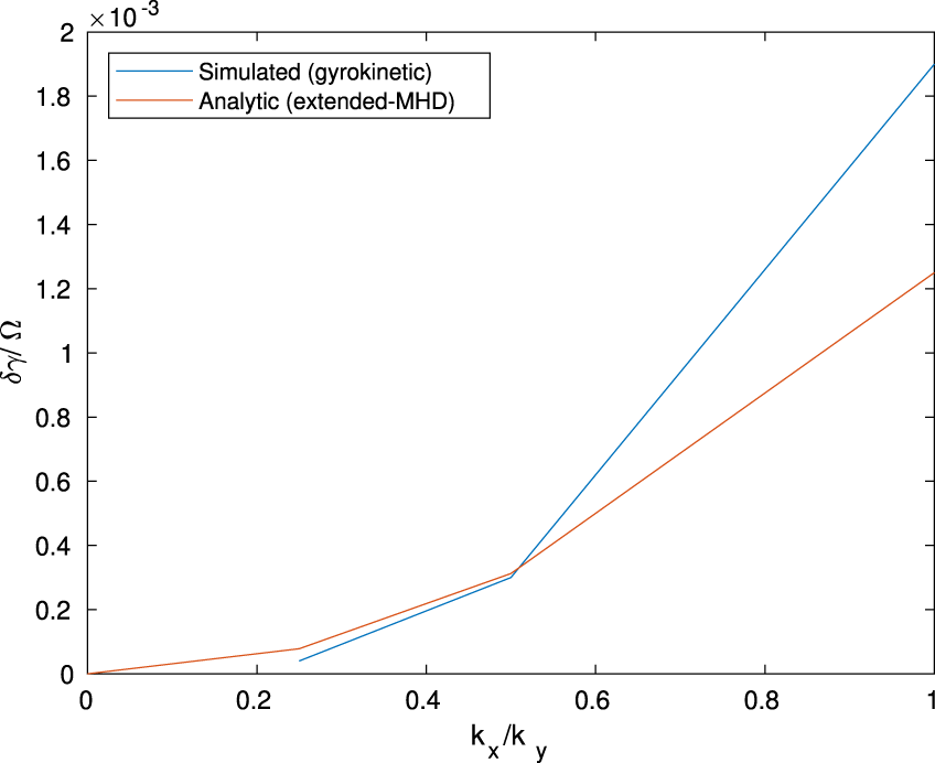
Figure 4. The difference between the growth-rate spectra for positive and negative parallel vorticity for the gyrokinetic simulation and analytic extended MHD (Nagano Reference Nagano1978). The simulation details are given in § 6.1.2 and  $k_{y}=2\unicode[STIX]{x03C0}/L_{y}$.
The dependence on the sign of the parallel vorticity is due to the chirality of gyromotion (Nagano Reference Nagano1978; Gingell et al. Reference Gingell, Chapman, Dendy and Brady2012). That is, the net flow depends on whether the shear flow and gyromotion are correspondent.
6.2 Blob motion
We examine the motion of a self-advecting blob of plasma, which initially consists of a pair of vortices of opposite sign. This is intended to be representative of the plasma blobs that form in the tokamak edge, driven by gradients in the plasma and magnetic field; as we are considering a simulation with a homogeneous  $B$ field, we will be simulating only the late-time behaviour of these blobs and ignoring the drive process itself (Krasheninnikov Reference Krasheninnikov2001). In the long-wavelength limit, the solutions of gyrokinetics are related to the Euler equation, which has solutions in terms of trajectory equations for localised vortices.
The simulations used gyrokinetic hydrogen ions,  $2^{26}$ markers, constant electron density, uniform background ion density, uniform ion and electron temperatures,
  $T_{\text{i}}=T_{\text{e}}$ and a time step equal to the thermal gyroperiod. The doubly periodic, two-dimensional spatial simulation domain used 256 grid points and a length of
  $L=80\unicode[STIX]{x03C0}\unicode[STIX]{x1D70C}_{\text{ti}}$ in each direction. The initialisation of
  $\unicode[STIX]{x1D6FF}f$ was given by
 $$\begin{eqnarray}\left.\begin{array}{@{}c@{}}\displaystyle \unicode[STIX]{x1D6FF}f=AF_{0}[d(\boldsymbol{R}-\boldsymbol{p}_{0}+\boldsymbol{d})-d(\boldsymbol{R}-\boldsymbol{p}_{0}-\boldsymbol{d})],\\ \displaystyle d(\boldsymbol{R})=\exp \left\{-\frac{R^{2}}{2\unicode[STIX]{x1D70E}_{\text{d}}^{2}}\right\}.\end{array}\right\}\end{eqnarray}$$
 For the simulations presented, we choose  $A=2.09\times 10^{-6}$,
  $y_{\text{d}}=L/16$,
  $\unicode[STIX]{x1D70E}_{\text{d}}=L/23.04$, the pair centre
  $\boldsymbol{p}_{0}=(L/10,L/2)$ and the vortex separation
  $\boldsymbol{d}=(0,y_{d})$.
The blob propagation for weak and strong flows is shown in figure 5. For weak flows, the dipole potential propagates in a straight line. An interpretation in terms of point vortices is that each vortex pulls the other around its centre, resulting in propagation. In the weak-flow limit, this motion is symmetrical, so each vortex is displaced an equal amount perpendicular to the line between the two vortices and the result is straight-line motion. For strong flows, the dipole propagates in a circle, instead: this is due to the effective  $E\times B$ drift speed being somewhat dependent on the sign of the parallel vorticity, so the top and bottom vortices move at different speeds. As the motion of each vortex stays perpendicular to the inter-vortex line, the resulting motion is on a curve. These effects are also observed with gyrofluid models (Madsen et al. Reference Madsen, Garcia, Stærk Larsen, Naulin, Nielsen and Rasmussen2011; Wiesenberger, Madsen & Kendl Reference Wiesenberger, Madsen and Kendl2014).
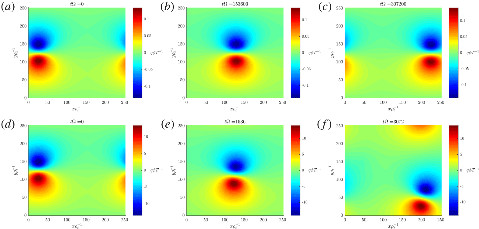
Figure 5. Electrostatic potential of the plasma blob on the doubly periodic, two-dimensional spatial simulation domain perpendicular to the slab magnetic field, for weak flows (a–c) and strong flows (d–f). Simulation details are described in § 6.2.
The radius of curvature of the curved path of the strong-flow blob  $R_{\text{b}}$ may be computed based on the relative speed of the two vortices and the distance between them. For circular motion about a common point collinear with the vortex pair, the velocities of the two vortices are
  $(R_{\text{b}}\pm y_{\text{d}})v_{\text{b}0}/R_{\text{b}}$, where
  $v_{\text{b}0}$ is the lowest-order blob speed (excluding the parallel vorticity dependence) and we solve to find
  $R_{\text{b}}$. We assume that the initial motion (figure 5) of the blob in the
  $y$ direction is small compared to that in the
  $x$ direction. This gives
 $$\begin{eqnarray}\frac{R_{\text{b}}}{v_{\text{b}0}}=\frac{y_{\text{d}}}{\unicode[STIX]{x1D6FF}v},\end{eqnarray}$$
 where  $\unicode[STIX]{x1D6FF}v$ is half the difference between the two vortex velocities.
The lowest-order blob velocity may be calculated by determining the electric field produced by each vortex and evaluating the  $\boldsymbol{E}\times \boldsymbol{B}$ motion on the other vortex, which is equal for the two vortices due to the symmetry of the setup. Assuming that the vortices retain their initial circular symmetry (which is justified for sufficiently small vortices), the velocity field outside a vortex at the origin in free space may be found as
  $\boldsymbol{v}=\hat{\unicode[STIX]{x1D73D}}K/R$, where
  $\hat{\unicode[STIX]{x1D73D}}$ is the angular unit vector,
  $K$ is a constant and
  $R$ is the distance from the vortex centre.
We have
 $$\begin{eqnarray}v_{\text{b}0}=u_{x\text{i}}-u_{x\text{s}},\end{eqnarray}$$
 where  $u_{x\text{i}}$ is the bulk inter-vortex flow speed in the
  $x$ direction,
  $u_{x\text{s}}$ is the bulk single-vortex flow speed in the
  $x$ direction,
 $$\begin{eqnarray}u_{x}=B^{-1}\unicode[STIX]{x2202}_{y}\unicode[STIX]{x1D719}\sim B^{-1}\unicode[STIX]{x1D719}/L_{y}\end{eqnarray}$$
 and  $L_{y}$ is the local length scale of variation of
  $\unicode[STIX]{x1D719}$ in the
  $y$ direction.
The strong-flow correction to the plasma equation of motion may be found by evaluating the third, strong-flow term in  $\dot{\boldsymbol{R}}$ (in (1.4)), by using that
  $B_{\Vert }^{\ast }-B$ (1.6) is small,
 $$\begin{eqnarray}\unicode[STIX]{x1D6FF}v\sim B^{-2}(B_{\Vert }^{\ast }-B)\dot{u}_{1},\end{eqnarray}$$
where
 $$\begin{eqnarray}B_{\Vert }^{\ast }-B\sim \dot{u}_{1}\sim \frac{u_{x\text{s}}}{L_{u}}\end{eqnarray}$$
 and  $L_{u}$ is the local length scale of variation of
  $u_{x\text{s}}$ in the
  $y$ direction.
The radius of curvature of the circular motion of the strong-flow blob expected from analysis is  $2.36\times 10^{3}\unicode[STIX]{x1D70C}_{\text{ti}}$ and we have reasonable agreement with the radius of curvature measured in simulations of
  $2.69\times 10^{3}\unicode[STIX]{x1D70C}_{\text{ti}}$.
7 Conclusions
We have described methods for the solution of gyrokinetic evolution equations where the field equations have a dependence on the time derivative of the field. Solutions consistent with the gyrokinetic ordering and the assumed smooth behaviour of trajectories in the limit of small  $\unicode[STIX]{x1D716}$ may be defined in terms of the limit of a Picard iteration procedure. Usually it will be possible in principle to transform coordinates so that the implicit dependence on the field does not arise, where a direct solution of the differential equation and the usual method of numerical solution are valid. It is, however, usually simpler to use the assumed asymptotic behaviour of the solution to directly construct solutions of equations derived from the symplectic form of the Lagrangian.
Implementation of this method for an electrostatic gyrokinetic formalism (Sharma & McMillan Reference Sharma and McMillan2015) is relatively straightforward, and we have illustrated that the code reduces to the usual weak-flow limit, and is also able to resolve dynamically evolving self-consistent strong flows. Although allowing time-evolving strong flows is interesting in itself, e.g. to allow the study of astrophysical structures and tokamak pedestals, this is mostly intended as a pathway to generalised electromagnetic gyrokinetic simulations. That is, implementing codes that allow large-scale MHD motion to be solved self-consistently together with microturbulence in a unified fashion; appropriate formalisms exist (McMillan & Sharma Reference McMillan and Sharma2016) that seem to be amenable to this approach, but have not yet been translated into numerical codes.
Acknowledgements
This work has been carried out within the framework of the EUROfusion consortium and has received funding from the Euratom research and training programme 2014–2018 under grant agreement no. 633053. The views and opinions expressed herein do not necessarily reflect those of the European Commission. This work was partly funded under EPSRC grant EP/N035178/1. Simulations were performed with the support of EUROfusion and Marconi Fusion.
Editor Per Helander thanks the referees for their advice in evaluating this article.


 Open access