Synoptic Measurements of Electron Temperature and Speed in the Solar Corona with Next Generation White-Light Coronagraph

Abstract

Current white-light coronagraphs measure polarized brightness (pB) of the solar corona using a single bandpass filter to measure the density of electrons. However, future coronagraphs can be modified to take pB images through four bandpass filters to measure density, temperature and speed of electrons. In this article, we use a spherical three dimensional coronal model of the Bastille Day coronal mass ejection to synthetically measure pB through four bandpass filters along lines of sight originating from two observers located diametrically in front (1 AU, 0, 0) and behind (-1 AU, 0, 0) the plane of the sky on the xy-ecliptic plane. The lines of sight pass through 81 positions on a straight line parallel to the solar north–south z-direction in the yz-plane and this line intersects the ecliptic at (0, $1.25~\mbox{R}_{\odot}$, 0) from Sun center. The 81 data points are separated in intervals of $0.05~\mbox{R}_{\odot}$ and points extend from (0, $1.25~\mbox{R}_{\odot}$, -$2.0~\mbox{R}_{\odot}$) to (0, $1.25~\mbox{R}_{\odot}$, $2.0~\mbox{R}_{\odot}$). The measured pB ratios are used to measure temperature and speed, then we compare with true temperature and speed in the plane of the sky, and quantify the difference, which is a systematic error associated with using modeled pB ratios, based on a symmetric corona, to compare with measured pB ratios, on an asymmetric corona. This understanding is reached by allowing the coronal model to rotate a full circle in intervals of $1^{\circ}$ and illuminating the lines of sight with both symmetric and asymmetric coronal atmospheres about the plane of the sky.

Appendix: Influence of Coronal Structure on Temperature and Speed Measurements for a Single Spacecraft

Here, in four steps we show the effect of streamers on measured temperature and speed using a simple streamer model in the shape of a fan.

• i) The symmetric corona is defined by a symmetric electron density profile (Equation 2 in article I), uniform temperatures (1.0 MK), and a uniform speed (200.0 $\mbox{km}\,\mbox{s}^{-1}$), and the corresponding measured (TSBR, SSBR) from Equation 1 in article I is (1.55, 1.237).

  In Figure 19 we plot modeled T-TSBR profile. The pair of wavelengths for the two filters used to model T-TSBR profile in Figure 19 were chosen from the temperature-dependent anti-nodes in the modeled pB spectra shown in Figure 1 in Reginald and Davila (2000). In Figure 19 we plot five model T-TSBR profiles for model temperature and speed ranging from [(0.06 MK → 10.0 Mk), (0.0 → 1000.0 $\mbox{km}\,\mbox{s}^{-1}$)], and the dotted profile in Figure 19, which is the average of the five model T-TSBR profiles is used represent the “speed independent” model T-TSBR profile to compare with measured TSBR to measure temperature. In Figure 19 the measured TSBR of 1.55 for the symmetric corona corresponds to a measured temperature of 1.0 MK.

  Figure 19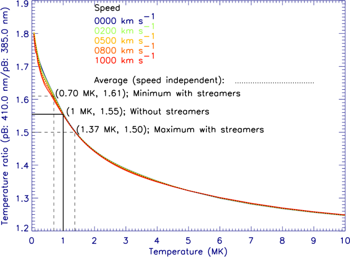

  

  Plot of the modeled T-TSBR profile (dotted black profile). The plot show coordinates of measured temperature (1.37 MK, 1.0 MK, 0.7 MK) corresponding to measured TSBR (1.50, 1.55, 1.61). Here, (1.0 MK, 1.55) corresponds to the symmetric corona while (1.37 MK, 1.50) and (0.7 MK, 1.61) corresponds to the maximum and minimum temperature for the asymmetric corona from Figure 22.

  In Figure 20 we plot modeled S-SSBR profile. The pair of wavelengths for the two filters used to model S-SSBR profile in Figure 20 were chosen from the temperature-independent nodes in the modeled pB spectra shown in Figure 2 in Reginald and Davila (2000). In Figure 20 we plot four model S-SSBR profiles for four assumed measured temperature 0.5, 1.0, 1.5, and 2.0 MK over model speed ranging from 0.0 to 1000.0 $\mbox{km}\,\mbox{s}^{-1}$. In Figure 20, which model S-SSBR profile should be used to compare with the measured SSBR? It is the model S-SSBR profile corresponding to the measured temperature. In Figure 20 the measured SSBR of 1.237 and measured temperature of 1.0 MK for the symmetric corona corresponds to a measured speed of 200.0 $\mbox{km}\,\mbox{s}^{-1}$.

  Figure 20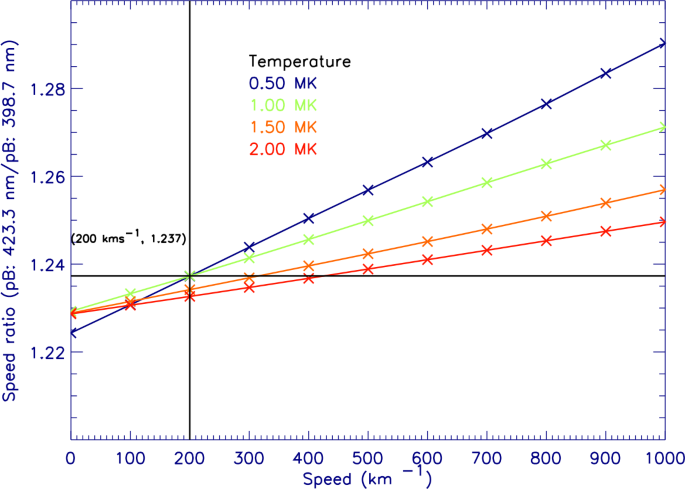

  

  Plots of the modeled S-SSBR profiles at measured temperatures 0.5, 1.0, 1.5, and 2.0 MK. The plot shows coordinates of measured speed (200.0 $\mbox{km}\,\mbox{s}^{-1}$) corresponding to measured SSBR (1.237) and measured temperature (1.0 MK) for the symmetric corona.

• ii) We introduce a simple model streamer in the shape of a fan as shown in Figure 21, which is characterized by its orientation with respect to the plane of the sky ($\xi$), angular width of the streamer ($\varepsilon$), and the density enhancement factor within the streamer (DE) over the ambient density given by Equation 2 in article II. For the streamer $\xi$ is allowed range up to $45^{\circ}$ in front and behind the plane of the sky in intervals of $5^{\circ}$, $\varepsilon$ is $20^{\circ}$, and DE is 10. The temperature and speed within the streamer still match the symmetric coronal environment of (1.0 MK, 200.0 $\mbox{km}\,\mbox{s}^{-1}$). What changes with the streamer is the shape of the density profile along the line of sight impacted by the streamer. In Figure 21 it is important to account for the location of NGC-A with respect to the plane of the sky, and check for scattering angle ($\Theta$) given by Equation 14 in Cram (1976) to (back, forward) scatter when the streamer is (behind, front) of the plane of the sky with respect to the observer. The coronal environment with the streamer will be called the asymmetric corona.

  Figure 21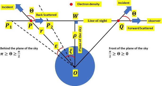

  

  Schematic of the streamer model, which is characterized by its orientation with respect to the plane of the sky ($\xi$), angular width of the streamer ($\varepsilon$), and the density enhancement factor within the streamer (DE) over the ambient density given by Equation 2 in article II.

• iii) The measured TSBR on symmetric and asymmetric corona are plotted in Figure 22 (left y-axis), which indicates that when the streamers are in (front, behind) the plane of the sky the measured TSBR for asymmetric corona are (>, <) compared to measured TSBR of 1.55 for symmetric corona. Also plotted in Figure 22 (right y-axis) are the measured temperature from comparing the measured TSBR with modeled T-TSBR in Figure 19 for both symmetric and asymmetric corona, which indicates that when the streamers are in (front, behind) the plane of the sky the measured temperature are (<, >) compared to measured temperature of 1.0 MK for symmetric corona. From Figure 22 the maximum and minimum measured temperature (1.37 MK, 0.70 MK) for asymmetric corona correspond to measured TSBR (1.50, 1.61).

  Figure 22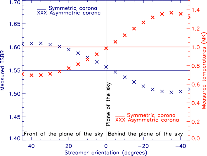

  

  Plot showing the measured TSBR for symmetric and asymmetric corona (left y-axis) and the corresponding measured temperature (right y-axis). The maximum and minimum measured TSBR are (1.61, 1.50), and the corresponding measured temperature from Figure 19 are (1.37 MK, 0.70 MK). Also shown by the horizontal lines are the measured (TSBR, temperature) of (1.55, 1.0 MK) for the symmetric corona.

• iv) The measured SSBR on symmetric and asymmetric corona are plotted in Figure 23 (left y-axis), and the corresponding measured speed are plotted in Figure 23 (right y-axis). These measured speed for the asymmetric corona were obtained by modeling S-SSBR profiles (not shown), for measured temperature in the asymmetric corona shown in Figure 22, and then comparing them with measured SSBR in Figure 23 (left y-axis). The maximum and minimum measured SSBR are (1.230, 1.242), and the corresponding measured speed are (30.0 $\mbox{km}\,\mbox{s}^{-1}$, 310.0 $\mbox{km}\,\mbox{s}^{-1}$).

  Figure 23

  

  Plot of the measured SSBR for symmetric and asymmetric corona (left y-axis) and the corresponding measured speed (right y-axis). The temperature were obtained from using Figure 19 to interpret the TSBR plotted Figure 22.

The highlights of the above example are the maximum (under-estimation, over-estimation) of measured temperature over the true temperature of 1.0 MK is (-0.30 MK, 0.37 MK), and the maximum (under-estimation, over-estimation) of measured speed over the true speed of 200.0 $\mbox{km}\,\mbox{s}^{-1}$ is (-170.0 $\mbox{km}\,\mbox{s}^{-1}$, 110.0 $\mbox{km}\,\mbox{s}^{-1}$).

Using only NGC-A, or a single spacecraft, can we use the under- and over-estimations of the measured temperature along some lines of sight as indicators for predicting the presence of coronal streamers, and its possible orientations with respect to the plane of the sky? To elaborate, let us assume NGC-A is flawless and the experiment functions as planned. Let us also assume two quiet regions, one each in solar east and west, and both regions have isothermal temperature of 1.0 MK. Then NGC-A would measure TSBR of 1.55 for both regions, which when compared with Figure 19 will measure temperature 1.0 MK. As long as the region remains undisturbed by streamers the measured TSBR will continue to measure 1.55. Now, if the measured TSBR rises in one region and falls in the other region, then from Figure 22 we can surmise on a possible streamer entering into the field of view and also predict its orientation with respect to the plane of the sky. When such streamers form they are not bound to disappear in a short span of time and with solar rotation their orientations with the plane of the sky will continue to change over time and reflect this change in measured TSBR. However, it is also possible a cosmic ray impinging on a pixel to also change the measured TSBR. In such cases, if the pixel is damaged, it will be visually recognized in pB images, and dark images taken from time to time with the aperture door closed to NGC-A to measure the dark noise of the detector. But, if the measured TSBR changes are due to statistical error (or photon noise), which will inevitably be present in a white-light coronagraph, then predictions are bound to fail. Then how do you address this issue? This issue is addressed at the design stage of NGC-A. Although we intend to measure pB the much dominant sources of brightness are the unpolarized F-coronal brightness and photospheric brightness diffracted off the occulter, which will be removed by the polarization camera, nevertheless, will be still contaminated by the statistical error associated with the unpolarized brightness. So the question is what fraction of the measured pB is due to statistical error? This fraction is quantified through rigorous signal to noise analysis to quantify the statistical error prior to finalizing the design of NGC-A. This analysis will determine how many images need to be co-added within acceptable temporal resolution, and how pixels in a given image be binned within acceptable spatial resolution. Finally, as a caution, Figure 5 in Cram (1976) also shows that the measured TSBR profiles will not necessarily have the same shape as shown in Figure 22 for different parameters used for the model streamer incorporated in to the model symmetric isothermal corona.

In the above narrative we referred to quiet regions as a region where the line of sight passing through that region will have a density profile that is symmetric about the plane of the sky, which we will not know with any certainty in remote measurements using a single spacecraft NGC-A. This fact is further compounded by the fact that in Figure 14 we will only have the blue curve pertaining to NGC-A. The question is: where on that blue curve can we assume that NGC-A is measuring the temperature in a quiet region? In this regard there is no straightforward answer but left to the observer’s judgment to set a benchmark after synoptic measurement of the temperature over at least one complete solar cycle. In support of deciding on this benchmark is the availability of over four million such blue curves in an example detector array of 2048 × 2048 $\text{pixel}^{2}$. The observer can then use the vast data set to compare with the images taken by NGC-A to group lines of sight in terms of their passages through conspicuous coronal structures such as streamers and CMEs and others that deem to bypass such areas in deciding on a benchmark temperature to reflect quiet regions. Of course, such benchmarks will always be subject to debate but will be deemed acceptable if the underlying arguments for demarcating a region as quiet are rationale and conform with the general attributes and definition of quiet region acceptable to the solar physics community. In any case, to win the debate, prediction on coronal structures need materialize at a higher certainty.

References

Altschuler, M.D., Newkirk, G.: 1969, Solar Phys.9, 131. DOI. ADS.
Billings, D.E.: 1966, A Guide to the Solar Corona, Academic Press, New York.
Crifo, E., Picat, J.P., Cailloux, M.: 1983, Solar Phys.83, 143. DOI. ADS.
Brueckner, G.E., Howard, R.A., Koomen, M.J., Korendyke, C.M., Michels, D.J., Moses, J.D., Socker, D.G., Dere, K.P., Lamy, P.L., Llebaria, A., Bout, M.V., Schwenn, R., Simnett, G.M., Bedford, D.K., Eyles, C.J.: 1995, Solar Phys.162, 357. DOI. ADS.
Fox, N.J., Velli, M.C., Bale, S.D., Decker, R., Driesman, A., Howard, R.A., Kasper, J.C., Kinnison, J., Kusterer, M., Lario, D., Lockwood, M.K., McComas, D.J., Raouafi, N.E., Szabo, A.: 2016, Space Sci. Rev.204, 7. DOI. ADS.
Hoeksema, J.T.: 1984, Structure and evolution of the large scale solar and heliospheric magnetic fields. Ph.D. thesis, Stanford Univ., ADS.
Howard, R.A., Moses, J.D., Vourlidas, A., Newmark, J.S., Socker, D.G., Plunkett, S.P., Korendyke, C.M., Cook, J.W., Hurley, A., Davila, J.M., Thompson, W.T., St. Cyr, O.C., Mentzell, E., Mehalick, K., Lemen, J.R., Wuelser, J.P., Duncan, D.W., Tarbell, T.D., Wolfson, C.J., Moore, A., Harrison, R.A., Waltham, N.R., Lang, J., Davis, C.J., Eyles, C.J., Mapson-Menard, H., Simnett, G.M., Halain, J.P., Defise, J.M., Mazy, E., Rochus, P., Mercier, R., Ravet, M.F., Delmotte, F., Auchere, F., Delaboudiniere, J.P., Bothmer, V., Deutsch, W., Wang, D., Rich, N., Cooper, S., Stephens, V., Maahs, G., Baugh, R., McMullin, D., Carter, T.: 2008, Space Sci. Rev.136, 67. DOI. ADS.
Lemaire, J.F., Stegen, K.: 2016, Solar Phys.291, 3659. DOI. ADS.
Müller, D., Marsden, R.G., St. Cyr, O.C., Gilbert, H.R.: 2013, Solar Phys.285, 25. DOI. ADS.
Reginald, N.L.: 2001, MACS, an instrument, and a methodology for simultaneous and global measurements of the coronal electron temperature and the solar wind velocity on the solar corona. Ph.D. thesis, Univ. of Delaware, ADS.
Reginald, N.L., Davila, J.M.: 2000, Solar Phys.195, 111. DOI. ADS.
Reginald, N.L., Newmark, J., Rastaetter, L.: 2019, Solar Phys.294, 100. DOI. ADS.
Reginald, N.L., Rastaetter, L.: 2019, Solar Phys.294, 12. DOI. ADS.
Reginald, N.L., Davila, J.M., St. Cyr, O.C., Rastaetter, L.: 2014, Solar Phys.289, 2021. DOI. ADS.
Reginald, N.L., St. Cyr, O.C., Davila, J.M., Rabin, D.M., Guhathakurta, M., Hassler, D.M.: 2009, Solar Phys.260, 347. DOI. ADS.
Reginald, N.L., St. Cyr, O.C., Davila, J.M., Rastaetter, L., Török, T.: 2018, Solar Phys.293, 82. DOI. ADS.
Schatten, K.H., Wilcox, J.M., Ness, N.F.: 1969, Solar Phys.6, 442. DOI. ADS.
Shklovskii, I.S.: 1965, Physics of the Solar Corona, Pergamon Press, Oxford. Edited by Beer, A., translated and edited by Meadows, A.J.
Török, T., Downs, C., Linker, J.A., Lionello, R., Titov, V.S., Mikić, Z., Riley, P., Caplan, R.M., Wijaya, J.: 2018, Astrophys. J.856, 75. DOI. ADS.
Wang, W.M., Sheeley, N.R.: 1992, Astrophys. J.392, 310. DOI. ADS.
Acknowledgements
We thank Predictive Science Inc. for sharing with us their Bastille Day CME model. NLR was supported by NASA grant PL10A-125. The authors thank the anonymous reviewer for the time and effort in reviewing our manuscript, requiring answers on the manuscript to probing questions on the material presented, highlighting mistakes, and suggesting alternate color schemes and language styles for clarity, which greatly improved the original manuscript submitted for review.
Author information
Authors and Affiliations
Corresponding author
Ethics declarations
Disclosure of Potential Conflicts of Interest
The authors declare that they have no conflicts of interest.
Additional information
Publisher’s Note
Springer Nature remains neutral with regard to jurisdictional claims in published maps and institutional affiliations.