Improving Density Peak Clustering by Automatic Peak Selection and Single Linkage Clustering

Abstract

Density peak clustering (DPC) is a density-based clustering method that has attracted much attention in the academic community. DPC works by first searching density peaks in the dataset, and then assigning each data point to the same cluster as its nearest higher-density point. One problem with DPC is the determination of the density peaks, where poor selection of the density peaks could yield poor clustering results. Another problem with DPC is its cluster assignment strategy, which often makes incorrect cluster assignments for data points that are far from their nearest higher-density points. This study modifies DPC and proposes a new clustering algorithm to resolve the above problems. The proposed algorithm uses the radius of the neighborhood to automatically select a set of the likely density peaks, which are far from their nearest higher-density points. Using the potential density peaks as the density peaks, it then applies DPC to yield the preliminary clustering results. Finally, it uses single-linkage clustering on the preliminary clustering results to reduce the number of clusters, if necessary. The proposed algorithm avoids the cluster assignment problem in DPC because the cluster assignments for the potential density peaks are based on single-linkage clustering, not based on DPC. Our performance study shows that the proposed algorithm outperforms DPC for datasets with irregularly shaped clusters.

1. Introduction

Clustering is the process of grouping data points such that each group contains similar data points, and the data points in different groups are dissimilar. It is the main task in data mining and has applications in many fields, such as marketing [1,2], image processing [3,4], bioinformatics [5] and finance [6]. For different applications, the notation of “similarity” or “dissimilarity” varies. For example, in customer segmentation, two customers are similar if they exhibit a similar spending profile, and thus the “distance” between their spending profiles is a good measure of dissimilarity. However, this distance may not be a good measure of dissimilarity for the application of identifying communities in a social network of people, where two persons in the same community are deemed similar. Notably, two persons far apart could be in the same community as long as there is a group of near-by persons between them. That is, a community is a densely populated region of people. For this type of application, the notion of similarity is related to the distance between the data points and the densities of the data points. Distance may also be defined differently for different applications. For example, symmetric distance is used for clustering analysis in [7].

Various clustering applications motivate the research community to develop many clustering methods to meet different clustering needs. Major clustering methods can be classified into the following categories: partitioning methods, hierarchical methods, density-based methods, grid-based methods, and model-based methods [8]. Partitioning methods aim to divide the data points in a dataset into k groups such that a specific objective function is minimized. The most commonly used partitioning method is k-means [9], representing each group by the centroid of the data points in the group, and tries to minimize the sum of the squared distance of each object to its group’s centroid. Hierarchical methods yield a dendrogram of data points showing how smaller groups are gradually combined to form larger groups (the agglomerative approach) or how larger groups are gradually divided into smaller groups (the divisive approach). Density-based methods form clusters by identifying those regions where the data points are densely populated. DBSCAN [10] and OPTICS [11] are two commonly used density-based methods. Grid-based methods place data points in a grid structure to accelerate the clustering process [12]. Model-based methods assume a mathematical model for each cluster and attempt to optimize the fit between the models and the clusters in the dataset. Please refer to [8,13,14] for a comprehensive survey of the clustering methods.

A density peak clustering (DPC) algorithm is a density-based clustering method proposed by Rodriguez and Laio [15] in 2014. Since its inception, DPC has received much attention in the research community [16,17,18,19,20,21,22,23,24,25,26,27,28,29,30]. Similar to other density-based methods, DPC calculates the density of each data point in the dataset. Unlike other density-based methods, DPC selects some data points in the dataset as the density peaks, forms a new cluster for each density peak, and assigns each non-peak data point to the same cluster as its nearest higher-density point in the dataset. However, DPC has two drawbacks. First, it is not trivial to select density peaks. Recall that each density peak forms a new cluster. If two data points that are supposed to be in the same cluster are both selected as the density peaks, they will be placed into two different clusters, yielding incorrect clustering results. Notably, DPC always selects the data point with the highest density as a density peak. Rodriguez and Laio [15] suggested selecting the remaining density peaks from those data points with high densities and are far from their nearest higher-density points. However, such a peak selection criterion is imprecise and prone to error. Figure 1 shows a directed graph where each vertex represents a data point in the Flame dataset [31], and each directed link connects a data point to its nearest higher-density point. Four of the directed links are highlighted in red to indicate those links whose starting points have high densities and are far from their nearest higher-density points. Selecting the data point with the highest density and the starting point of any of these four directed links as the density peaks, DPC will break the lower portion of the Flame dataset into more than one group, yielding poor clustering results.

Another drawback with DPC is its cluster assignment strategy, which assigns a non-peak data point and its nearest higher-density point into the same cluster. This strategy works fine for those data points that are not far from their nearest higher-density point. However, for those data points that are far from their nearest higher-density point, this strategy often yields a poor cluster assignment. For example, consider the three longest red directed links in Figure 1. If the starting point and the ending point of any of the three directed links are placed into the same cluster, DPC will incorrectly place the entire upper portion and part of the lower portion of the Flame dataset into one cluster.

The objective of this study is to eliminate the above two drawbacks of DPC. We propose a new clustering method that integrates DPC and single linkage clustering [8]. The proposed method automatically determines a set of potential density peaks by choosing those data points far from their nearest higher-density points. Notably, we use the term “potential” density peaks because this set may also contain the outliers of the dataset. The proposed method adopts the cluster assignment strategy of DPC only for those data points not far from their nearest higher-density points. Consequently, the proposed method will not yield the four red directed links in Figure 1. For those data points far away from their nearest higher-density points, single linkage clustering is adopted to reduce the number of clusters further.

The rest of this paper is organized as follows. Section 2 describes DPC and reviews related work. Section 3 proposes our method, and Section 4 presents the experimental results. Finally, Section 5 concludes this study.

2. Related Work

2.1. Density Peak Clustering (DPC)

The DPC algorithm contains several major steps: calculating density and searching the nearest higher-density point for each point in the dataset, selecting density peaks, and assigning clusters. This section describes these steps in detail.

The density of a point is based on a user-specified parameter $d_c$ representing the radius of a point’s neighborhood. Given a data set $X$, the local density $\mathsf{\rho }\left(x_i\right)$ of a point $x_i\in X$ can be calculated as the number of points within the neighborhood of $x_i$, as shown below.

$$\mathsf{\rho }\left(x_i\right)={{\displaystyle \sum }}_{x_j\in X\backslash \left\{x_i\right\}}\chi \left(d\left(x_i, x_j\right)-d_c\right)$$

(1)

where $d\left(x_i, x_j\right)$ is the Euclidean distance between points $x_i$ and $x_j$, and $\chi \left(t\right)=1$ if $t<0$ and otherwise $\chi \left(t\right)=0$. For small data sets, Rodriguez and Laio [15] suggested using an exponential kernel for calculating density, as shown below.

$$\mathsf{\rho }\left(x_i\right)={{\displaystyle \sum }}_{x_j\in X\backslash \left\{x_i\right\}}exp\left(-\frac{{\left(d\left(x_i, x_j\right)\right)}^2}{{\left(d_c\right)}^2}\right)$$

(2)

The value of $d_c$ can be set to the lower p% of all distances between any two points in $X$. Consequently, the average number of neighbors of a point is about p% of the total number of points in $X$. Notably, point $x_j$ is a neighbor of point $x_i$ if $d\left(x_i, x_j\right)<d_c$. Rodriguez and Laio [15] suggested using $1\le p\le 2$.

Let $\mathsf{\delta }\left(x_i\right)$ denote the distance between point $x_i$ and the nearest higher-density point of $x_i$. Then, $\mathsf{\delta }\left(x_i\right)$ can be calculated as follows.

$$\mathsf{\delta }\left(x_i\right)=\{\begin{array}{cc}\underset{x_j\in X \wedge \mathsf{\rho }\left(x_j\right)>\mathsf{\rho }\left(x_i\right)}{\min }d\left(x_i,x_j\right),& \mathrm{if} \mathsf{\rho }\left(x_i\right)<\underset{x_j\in X}{\max }\mathsf{\rho }\left(x_j\right)\hfill \\ \underset{x_j\in X}{\max }d\left(x_i,x_j\right),& \mathrm{otherwise}.\hfill \end{array}$$

(3)

Notably, for the point with the highest density in $X$, $\mathsf{\delta }\left(x_i\right)$ is set to the largest distance between any two points in $X$, as shown in the second case of (3). For ease of illustration, $\mathsf{\sigma }\left(x_i\right)$ is used to denote the nearest higher-density point of $x_i$. That is:

$$\mathsf{\sigma }\left(x_i\right)=\{\begin{array}{cc}\underset{x_j\in X \wedge \mathsf{\rho }\left(x_j\right)>\mathsf{\rho }\left(x_i\right)}{\mathrm{argmin}}d\left(x_i,x_j\right),& \mathrm{if} \mathsf{\rho }\left(x_i\right)<\underset{x_j\in X}{\max }\mathsf{\rho }\left(x_j\right)\hfill \\ x_i,& \mathrm{otherwise}.\hfill \end{array}$$

(4)

The data point with the highest density does not have any higher-density point, so for this data point, we set $\mathsf{\sigma }\left(x_i\right)$ to $x_i$, as shown in the second case of (4).

Once $\mathsf{\rho }\left(x_i\right)$ and $\mathsf{\delta }\left(x_i\right)$ are available for each point $x_i\in X$, Rodriguez and Laio [15] suggested selecting those points with high $\mathsf{\rho }\left(x_i\right)$ and high $\mathsf{\delta }\left(x_i\right)$ as density peaks. One way to achieve this is to select those points with $\mathsf{\gamma }\left(x_i\right)$ greater than a specified threshold where $\mathsf{\gamma }\left(x_i\right)=\mathsf{\rho }\left(x_i\right)\mathsf{\delta }\left(x_i\right)$. One problem with this method is that $\mathsf{\rho }\left(x_i\right)$ and $\mathsf{\delta }\left(x_i\right)$ are on different scales, and one of them may dominate the ordering of $\mathsf{\gamma }\left(x_i\right)$, resulting in a poor selection of density peaks. Another way is to select the density peaks manually with the assistance of the decision graph [15], a two-dimensional graph with $\mathsf{\rho }\left(x_i\right)$ and $\mathsf{\delta }\left(x_i\right)$ as the horizontal and vertical coordinates, respectively. However, it remains a difficult and ineffective way to select the density peaks.

After the density peaks have been determined, the cluster assignment can proceed straightforwardly. Suppose that k points are selected as the density peaks. First, each density peak forms a new cluster, with a cluster label from one to k. Let $\mathsf{\eta }\left(x_i\right)$ denote the cluster label of the cluster containing point $x_i$. Because each non-peak point $x_i$ is assigned to the same cluster as its nearest higher-density point $\mathsf{\sigma }\left(x_i\right)$, $\mathsf{\eta }\left(x_i\right)$ can be determined as follows:

$$\mathsf{\eta }\left(x_i\right)=\mathsf{\eta }\left(\mathsf{\sigma }\left(x_i\right)\right)$$

(5)

Notably, because (5) is recursive, we must ensure that $\mathsf{\eta }\left(\mathsf{\sigma }\left(x_i\right)\right)$ is calculated before $\mathsf{\eta }\left(x_i\right)$. This can be achieved by performing the cluster assignment for the non-peak points by the descending order of their densities. Figure 2 shows the DPC algorithm.

Figure 3 illustrates the clustering process of DPC using a directed tree with a sink vertex. Each vertex represents a point in the dataset, each directed link connects a point to its nearest higher-density point, and the sink vertex is the point with the highest density in the dataset. After selecting the density peaks (i.e., the red vertices in Figure 3), DPC decomposes the directed tree into the same number of directed sub-trees. Each of the subtrees has its sink vertex at a density peak. All points in a subtree form a cluster (shown as a gray ellipse region in Figure 3).

2.2. Variants of DPC

DPC has received much attention in the research community, and many variants of DPC have been proposed. This section reviews them from three perspectives: parameter setting, density peak selection, and computation acceleration.

Because DPC’s parameters can affect the clustering performance, many studies focused on setting these parameters properly. For example, ref. [16] applied the concept of heat diffusion and [17] employed the potential entropy of the data field to assist in setting the radius $d_c$. Also, many studies suggested using k nearest neighbors to define density, instead of using the radius $d_c$ [18,19,20,21]. Furthermore, ref. [22] suggested calculating two kinds of densities, one based on k nearest neighbors and one based on local spatial position deviation, to handle datasets with mixed density clusters.

As described in Section 1, selecting the density peaks in DPC can be difficult and ineffective. To resolve this problem, ref. [23] proposed a comparative technique to choose the density peaks, ref. [24] estimated density dips between points to determine the number of clusters, and [25] applied data detection to determine density peaks automatically. In [21], the optimal number of clusters was extracted from the results of hierarchical clustering. Furthermore, it may be more suitable for some datasets to locate a cluster by more than one density peak [26,27]. Overall speaking, making the clustering process more adaptive to the datasets with less human intervention is the goal.

Several studies focused on accelerating DPC [28,29,30]. Recall that DPC needs to search the nearest higher-density point $\mathsf{\sigma }\left(x_i\right)$ for each point $x_i$ (see Equation (4)). For each point $x_i$ whose density is not the highest within its neighborhood, ref. [28] suggested that we can omit this step by simply setting $\mathsf{\sigma }\left(x_i\right)$ to the point with the highest density within the neighborhood of $x_i$. Because most points are not the point with the highest density in their respective neighborhoods, this method accelerates calculating $\mathsf{\sigma }\left(x_i\right)$ in DPC. Alternatively, ref. [29] accelerates calculating the density $\mathsf{\rho }\left(x_i\right)$ by integrating k-means with DPC. Also, ref. [30] used k nearest neighbors to accelerate the calculation of both $\mathsf{\rho }\left(x_i\right)$ and $\mathsf{\delta }\left(x_i\right)$.

3. The Proposed Method

This section describes the proposed method that avoids DPC’s drawbacks described in Section 1. Specifically, the proposed method does not need to manually select the density peaks and does not place a point and its nearest higher-density point in the same cluster if the two points are far apart. The proposed method contains five stages: build a directed tree, remove long links, generate preliminary clustering, apply hierarchical clustering to the forest, and generate flat clustering results. The proposed method, referred to as density peak single linkage clustering (DPSLC), is shown in Figure 4.

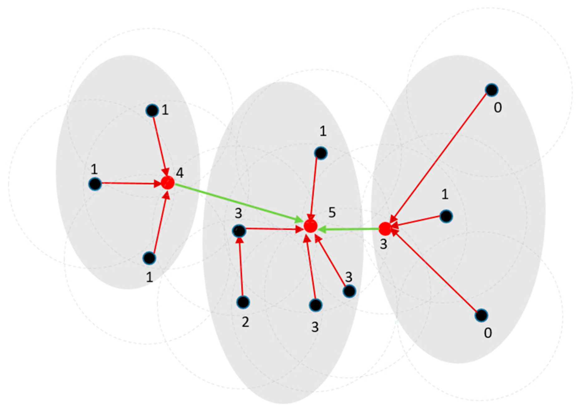
Recall from Section 2.1 and Figure 3 that DPC constructs a directed tree with a sink vertex. As with DPC, Stage 1 of DPSLC also constructs a directed tree. Figure 5 shows an example where each filled circle and the integer next to it represent a point and the point’s density (based on Equation (1)), respectively, and each red dashed circle shows the neighborhood of a point. Each link connects a point to its nearest higher-density point; the red filled circle is the point with the highest density, which is also the sink vertex of the directed tree.

Stage 2 of DPSLC decomposes the directed tree into a forest of directed subtrees by removing those links that are too long. Specifically, DPSLC removes the link $x_i\to x_j$ if $d\left(x_i,x_j\right)\ge 2.1d_c$. Stage 2 of DPSLC will delete the three non-black links in Figure 5. The green link illustrates the case of linking from an outlier; the purple link illustrates the case of linking from a high-density point to its nearest higher-density point that is far away. Removing these two types of links allows DPSLC to break the connection between two regions that are not densely connected. The blue link connects the blue point to its nearest higher-density point, making the blue point connect to the gray region on the right in Figure 5. However, the two neighbors (within the red-dashed circle centered at the blue point) of the blue point are connecting to the gray region on the left in Figure 5. Thus, removing this blue link allows DPSLC to break the connection between the blue point and the right gray region, and yield a new region containing only the blue point. This new region will be combined with other regions later in Stage 4. After Stage 2, DPSLC yields a forest of four directed trees (shown in gray regions) in Figure 5.

Stage 3 of DPSLC constructs a preliminary clustering result by forming a cluster for each directed tree in the forest. The four gray regions in Figure 5 show the four clusters generated in this stage.

Let ${\mathit{C}}_i$ and ${\mathit{C}}_j$ be two clusters in the preliminary clustering result of Stage 3. The single-linkage distance ${∆}^S\left({\mathit{C}}_i,{\mathit{C}}_j\right)$ between ${\mathit{C}}_i$ and ${\mathit{C}}_j$ is the distance between two points (one in each cluster) that are closest to each other. The overlapping distance ${∆}^O\left({\mathit{C}}_i,{\mathit{C}}_j\right)$ between ${\mathit{C}}_i$ and ${\mathit{C}}_j$ is the reciprocal of one plus the number of point pairs $\left(x_i,x_j\right)$ satisfying $d\left(x_i,x_j\right)<2d_c$ for $x_i\in {\mathit{C}}_i$ and $x_j\in {\mathit{C}}_j.$

$${∆}^S\left({\mathit{C}}_i,{\mathit{C}}_j\right)=\min \left\{d\left(x_i,x_j\right)|x_i\in {\mathit{C}}_i\wedge x_j\in {\mathit{C}}_j\right\}$$

(6)

$${∆}^O\left({\mathit{C}}_i,{\mathit{C}}_j\right)={\left(1+\left|\left\{\left(x_i,x_j\right)|d\left(x_i,x_j\right)<2d_c \wedge x_i\in {\mathit{C}}_i \wedge x_j\in {\mathit{C}}_j\right\}\right|\right)}^{-1}$$

(7)

Stage 4 of DPSLC performs agglomerative clustering on the preliminary clustering result of Stage 3 based on the single-linkage distance or the overlapping distance defined in (6) and (7). Here, overlapping distance is suitable for most datasets. However, for highly unbalanced datasets, single-linkage distance is preferred. The two nearest clusters are repeatedly combined into one until there is only one cluster left, and a dendrogram is generated to show the hierarchical relationship among clusters.

Figure 6 shows the dendrogram for the example in Figure 5. The red, green, and purple links in Figure 6 are the three shortest single-linkage distances adopted in the dendrogram. Notably, the number of clusters in the preliminary clustering result generated in Stage 3 is usually small, so the hierarchical clustering in Stage 4 will not consume too much time.

Stage 5 of DPSLC retrieves a flat clustering result from the hierarchical clustering result of Stage 4. Given the desired number of clusters k, this can be done by a horizontal cut on the dendrogram generated in Stage 4. For example, in Figure 6, setting the distance between clusters to a and b results in two and three clusters, respectively.

Additional parameter min_pts can be used to enforce that the clustering result contains k large clusters, each with no fewer than min_pts points, and possibly, some small clusters for outliers in the dataset.

4. Performance Study

4.1. Test Datasets

In this study, we used 12 well-known two-dimensional synthetic datasets to demonstrate the performance of the proposed algorithm.

Table 1. Number of points and number of clusters in the 12 datasets.

Dataset	Number of Clusters	Number of Points
Spiral	3	312
R15	15	600
D31	31	3100
A1	20	3000
T2000	2	2000
T1000	2	1000
T300	2	300
Flame	2	240
Aggregation	7	788
Jain	2	373
SMS02	3	1000
Unbalance	8	6500

describes the number of clusters and the number of points in these datasets. See Appendix A for the data distribution of these datasets.

Dataset Spiral [32] consists of three spiral-shaped clusters. Dataset R15 [33] consists of 15 similar Gaussian clusters positioned on concentric circles. Dataset D31 [33] consists of 31 similar Gaussian clusters positioned along random curves. Dataset A1 [34] contains 20 circular clusters, where each cluster has 150 points. Datasets T300, T1000, and T2000 contain two half-ring-shaped clusters each, where the density is T300 < T1000 < T2000. Dataset Flame [31] consists of two non-Gaussian clusters of points, where both clusters are of different sizes and shapes. Dataset Aggregation [35] consists of seven perceptually distinct (non-Gaussian) clusters of points. Dataset Jain [36] consists of two crescent-shaped clusters with different densities. Dataset SMS02 consists of three rectangular-shaped clusters with different sizes. Dataset Unbalance consists of eight clusters, where three of them are dense, and the other five are sparse.

4.2. Experiment Setup

Table 2. Parameter setting of DPSLC.

Parameter	Value	Description
$p$	2	$p$ is used to determine the radius $d_c$ of the neighborhood
k	See Table 1	The number of clusters in a dataset
min_pts	2	The minimum number of points in a cluster
cluster_distance	overlapping distance or single-linkage distance	Use overlapping distance for all datasets except the dataset Unbalance, which uses single-linkage distance.

shows the parameter setting of DPSLC. Parameter p = 2 is adopted to determine the radius $d_c$ of the neighborhood, as described in Section 2.1. The number of clusters k is set to the exact number of clusters in the dataset, as specified in Table 1. Parameter min_pts is set to two, so the final clustering result contains k large clusters (each with no fewer than min_pts points) and possibly, some small clusters of outliers. For all datasets except the dataset Unbalance, overlapping distance (see Equation (7)) is adopted to calculate the distance between two clusters in the preliminary clustering results generated at Stage 3 of DPSLC. Because Database Unbalance contains clusters of extremely different densities, single-linkage distance is adopted instead.

The experiment compares the performance of DPSLC and DPC.

Table 3. Parameter setting of DPC.

Parameter	Value	Description
$p$	2	$p$ is used to determine the radius $d_c$ of the neighborhood
k	See Table 1	The number of clusters in a dataset

shows the parameter setting of DPC. Parameter p is set to two, the same as in DPSLC. The top k data points with the highest $\mathsf{\gamma }\left(x_i\right)$ are selected as the density peaks, where $\mathsf{\gamma }\left(x_i\right)=\mathsf{\rho }\left(x_i\right)\mathsf{\delta }\left(x_i\right)$ and k is set to the exact number of clusters in the dataset, as specified in Table 1.

For each dataset, the clustering result C of DPSLC or DPC is compared against the ground truth T. The following four measures are collected:

• Homogeneity score measures the data points in the same cluster according to C are indeed in the same cluster according to the ground truth T. Homogeneity score is between 0 and 1, and 1 represents that C is perfectly homogeneous labeling.
• Completeness score measures the data points in the same cluster according to the ground truth T are placed in the same cluster according to C. Completeness score is between 0 and 1, and 1 represents that C is perfectly complete labeling.
• Adjusted Rand index (ARI) = (RI – Expected _Value(RI))/(max(RI) – Expected _Value(RI)), where RI (short for Rand index) is a similarity measure between two clustering results of the same dataset by considering all pairs of data points that are assigned in the same or different clusters in the two clustering results. ARI adjusts RI for chance such that random clustering results have an ARI close to 0. ARI can yield negative values if RI is less than the expected value of RI. When two clustering results are identical, ARI = 1.
• Adjusted mutual information (AMI) adjusts mutual information (MI) to correct the agreement’s effect due to chance. Similar to ARI, random clustering results have an AMI close to 0. When two clustering results are identical, AMI = 1.

4.3. Experiment Results

Table 4. Performance results of the 12 datasets. ARI: adjusted Rand index; AMI: adjusted mutual information.

Dataset	DPSLC				DPC
	Homogeneity	Completeness	ARI	AMI	Homogeneity	Completeness	ARI	AMI
Spiral	1.000	1.000	1.000	1.000	1.000	1.000	1.000	1.000
R15	0.994	0.994	0.993	0.994	0.994	0.994	0.993	0.994
D31	0.957	0.957	0.935	0.955	0.957	0.957	0.935	0.955
A1	0.970	0.970	0.959	0.970	0.970	0.970	0.959	0.970
T2000	0.930	0.930	0.966	0.930	0.930	0.930	0.966	0.930
T1000	0.941	0.941	0.972	0.941	0.941	0.941	0.972	0.941
T300	1.000	1.000	1.000	1.000	0.439	0.484	0.416	0.438
Flame	1.0	0.943	0.988	0.942	0.422	0.405	0.327	0.403
Aggregation	0.993	0.992	0.996	0.992	0.982	0.861	0.755	0.860
Jain	1.000	1.000	1.000	1.000	0.637	0.560	0.644	0.559
SMS02	0.975	0.978	0.991	0.975	0.727	1.000	0.822	0.727
Unbalance	1.000	0.999	1.000	0.999	0.970	0.824	0.853	0.823

shows the performance results. DPSLC and DPC yield the same clustering results for the first six datasets in Table 4. The common characteristics of these six datasets are that they contain clusters that are nicely separated and with similar densities. Both approaches achieve excellent performance on these six datasets.

DPSLC outperforms DPC on the bottom six datasets in Table 4. The clusters in each of these six datasets are either not well separated or with very different densities. DPC performs poorly on these datasets, but DPSLC can still achieve excellent clustering results. The rest of this section inspects the process of DPSLC for these datasets. The DPC’s clustering results are presented in Appendix B.

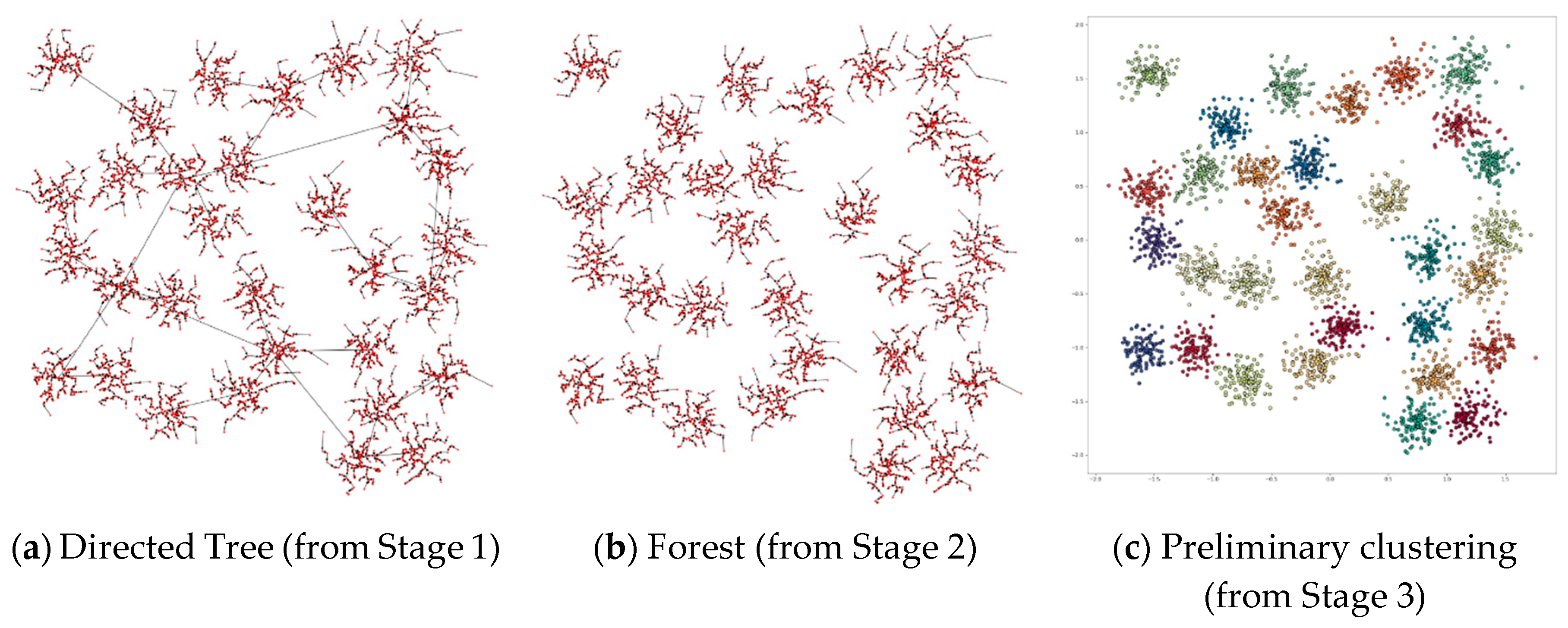
4.3.1. Applying DPSLC on Dataset T300

Figure 7 shows the process of applying DPSLC on dataset T300. The directed tree generated in Stage 1 contains several long links (see Figure 7a), which are subsequently removed in Stage 2 (see Figure 7b). The preliminary clustering result contains eight clusters where the star symbols indicate the positions of the density peaks (see Figure 7c). The final clustering result contains two clusters.

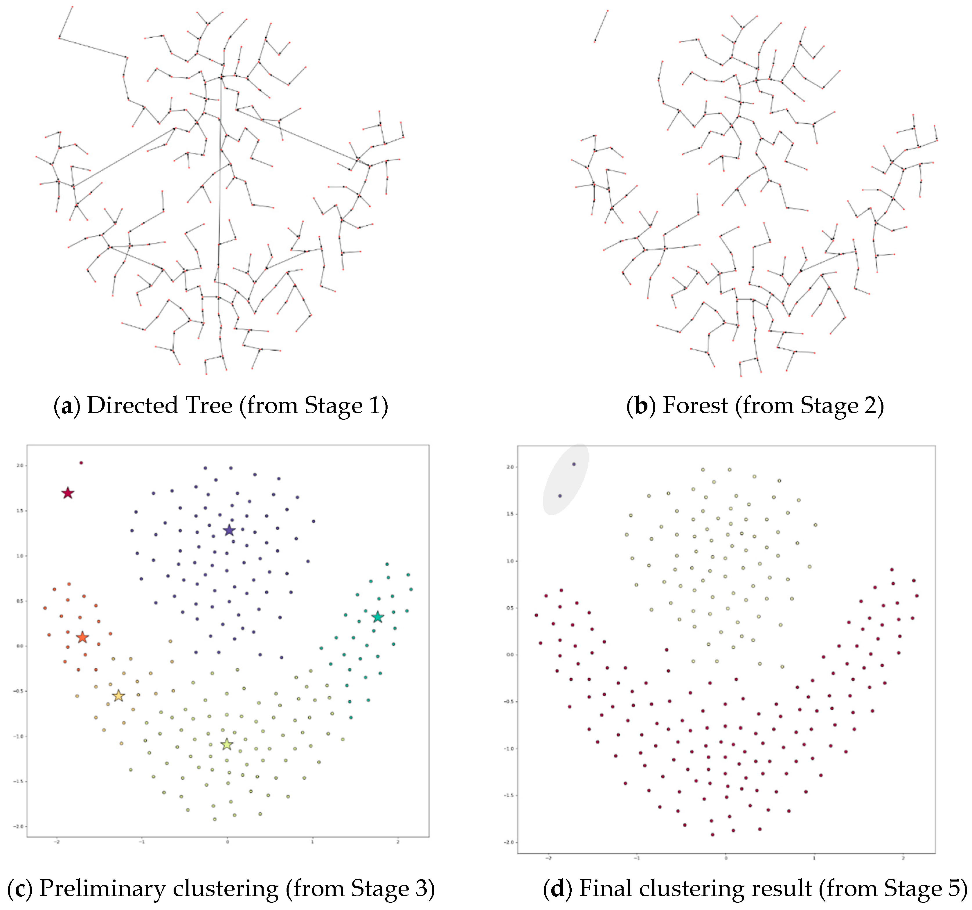
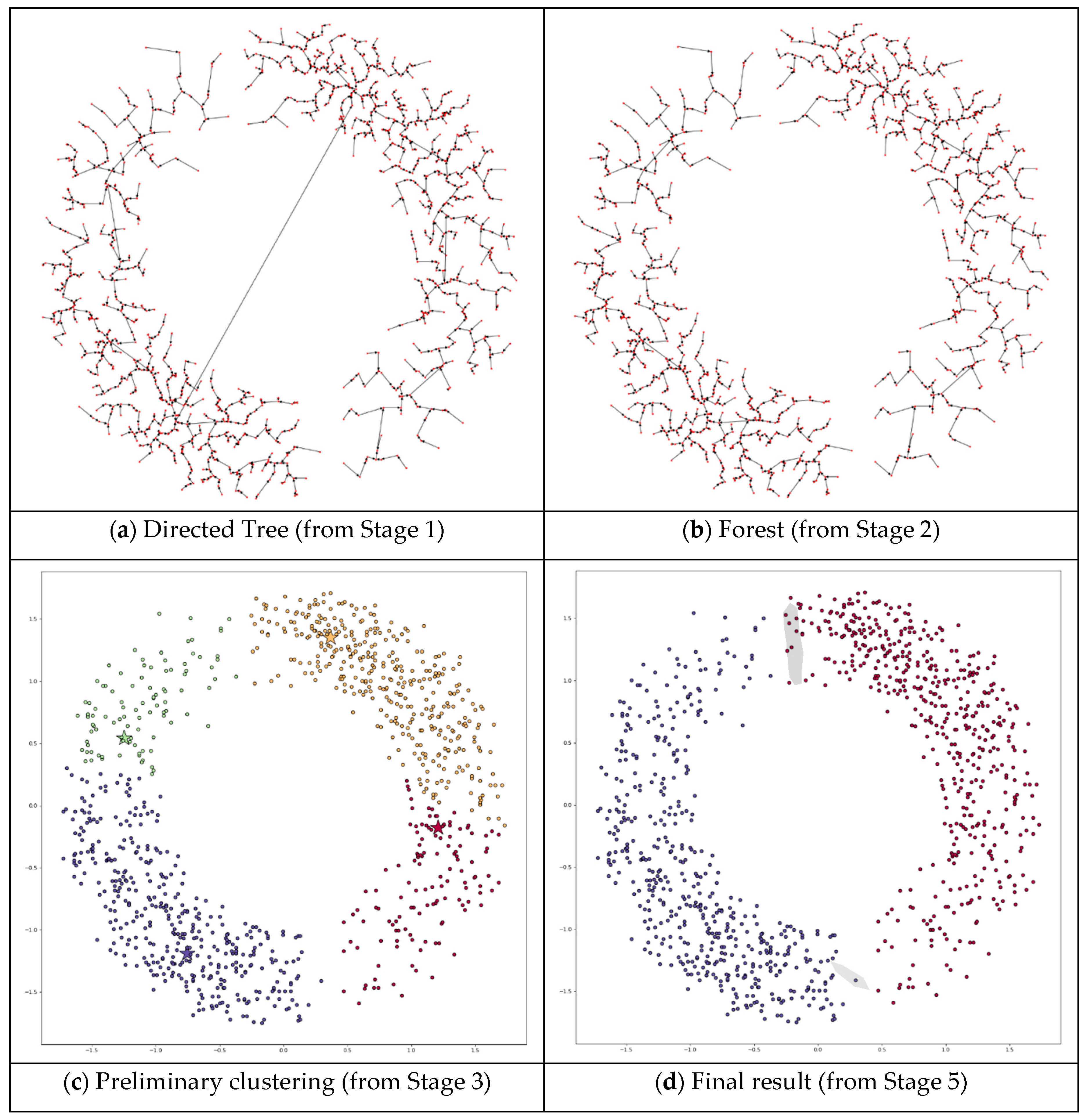
4.3.2. Applying DPSLC on Dataset Flame

Figure 8 shows the process of applying DPSLC on dataset Flame. Notice that the preliminary clustering result contains six clusters, including a cluster of two outliers in the top left corner (see Figure 8c). The final clustering result includes two large clusters and a small cluster of outliers (shown in the gray region in Figure 8d).

4.3.3. Applying DPSLC on Dataset Aggregation

Figure 9 shows the process of applying DPSLC on dataset Aggregation. According to the ground truth in Figure A1i, the two data points placed in the wrong clusters by DPSLC are shown in the gray region in Figure 9d.

4.3.4. Applying DPSLC on Dataset Jain

Figure 10 shows the process of applying DPSLC on dataset Jain. Dataset Jain contains one dense region and one sparse region. DPSLC breaks the dataset into 15 small groups in the preliminary clustering result (see Figure 10c) and coalesces them into two clusters in the final result (see Figure 10d).

4.3.5. Applying DPSLC on Dataset SMS02

Figure 11 shows the process of applying DPSLC on dataset SMS02. According to the ground truth in Figure A1k, the four data points placed in the wrong clusters by DPSLC are shown in the gray region in Figure 11d.

4.3.6. Applying DPSLC on Dataset Unbalance

Figure 12 shows the process of applying DPSLC on dataset Unbalance, which contains three dense regions and five sparse regions. The densities of the density regions and the sparse regions differ significantly. Consequently, setting parameter p = 2 results in a small value for $d_c$, which yields many clusters with just one point in the sparse regions at Stage 3 of DPSLC, as shown in Figure 12c. However, most of these clusters correctly coalesce at Stage 5 of DPSLC. However, there are still two data points misidentified as outliers by DPSLC, shown in the gray region in Figure 12d.

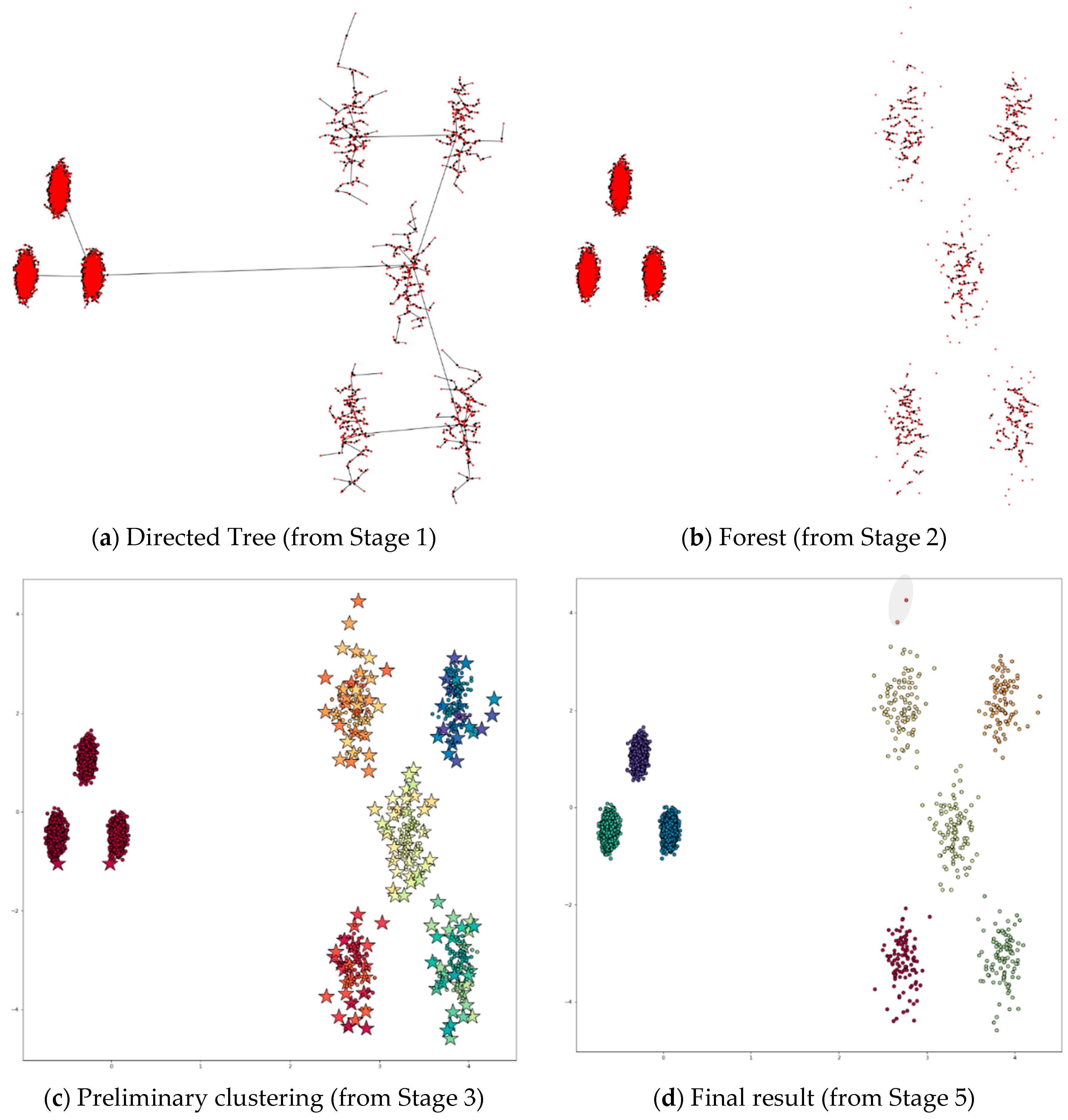
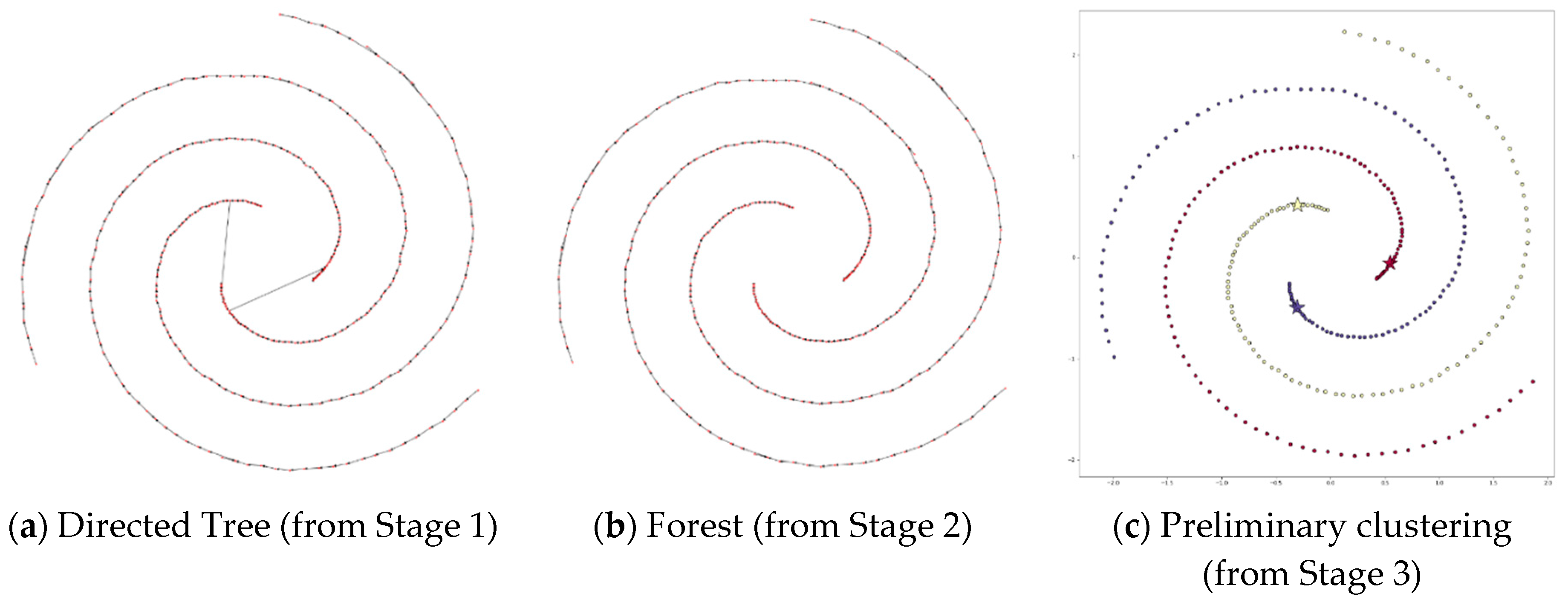
4.3.7. Applying DPSLC on Datasets Spiral, R15, D31, A1, T2000, and T1000

Figure 13, Figure 14, Figure 15, Figure 16, Figure 17 and Figure 18 show the process of applying DPSLC on datasets Spiral, R15, D31, A1, T2000, and T1000, respectively. For datasets Spiral, R15, D31, and A1, DPSLC ends at Stage 3 because the number of clusters has reached the desired k value.

The two gray regions in Figure 17d and two gray regions in Figure 18d indicate data points where the results of DPSLC and the ground truth disagree. We manually inspect those data points in Figure 17d and Figure 18d against their ground truth in Figure A1e,f. It appears that the DPSLC makes a better cluster assignment than the ground truth does for those data points.

5. Conclusions

This paper proposes DPSLC to improve DPC. DPSLC effectively avoids assigning a data point to the same cluster as its nearest higher-density point if both points are far apart. However, such a strategy could also yield many small clusters. For example, in the preliminary clustering result of dataset Unbalance, many small clusters appear on the right half of Figure 12c. DPSLC conquers this problem by applying single-linkage agglomerative clustering on the preliminary clustering result. The performance results in Table 4 show that DPSLC can still perform well on those datasets that DPC fails short.

Density-based clustering approaches are based on the idea of searching dense regions in a dataset. However, there is no de facto standard for what constitutes a dense region. In this study, we use a radius $d_c$ to define the neighborhood, and subsequently, calculate the density of a data point [10,15]. Some other studies calculate the density of a data point using the distance to the data point’s k nearest neighbor [18,19,20,21]. However, the proper value for either $d_c$ or k depends on the characteristic of the dataset. Thus, clustering approaches whose value for $d_c$ or k is adaptive to the dataset are worthy of investigation. In this study, we set the value of $d_c$ so that each data point has about 2% of all data points within its neighborhood, on average. Thus, the value of $d_c$ is adaptive to the dataset to a small extent. However, more sophisticated strategies are needed.

Finally, using a single $d_c$ or k may be insufficient for those datasets containing clusters with a wide range of densities. Using multiple $d_c$ or k may be a better way to capture the patterns of these clusters. For example, persistent homology detects persistent topological features by inspecting data points over a wide range of scales [37]. Similarly, DPC can experiment with a wide range of $d_c$ or k to detect the persistent clustering among data points. Alternatively, future research directions can also consider the integration use of $d_c$ and k.

References

- Wang, G.; Li, F.; Zhang, P.; Tian, Y.; Shi, Y. Data Mining for Customer Segmentation in Personal Financial Market. In Proceedings of International Conference on Multiple Criteria Decision Making; Springer: Berlin/Heidelberg, Germany, 2009; pp. 614–621. [Google Scholar]
- Arabie, P.; Carroll, J.D.; DeSarbo, W.; Wind, J. Overlapping Clustering: A New Method for Product Positioning. J. Mark. Res. 1981, 18, 310–317. [Google Scholar] [CrossRef]
- Chen, Z.; Qi, Z.; Meng, F.; Cui, L.; Shi, Y. Image Segmentation via Improving Clustering Algorithms with Density and Distance. Procedia Comput. Sci. 2015, 55, 1015–1022. [Google Scholar] [CrossRef] [Green Version]
- Filipovych, R.; Resnick, S.M.; Davatzikos, C. Semi-supervised cluster analysis of imaging data. Neuroimage 2011, 54, 2185–2197. [Google Scholar] [CrossRef] [PubMed] [Green Version]
- Lowe, R.; Shirley, N.; Bleackley, M.; Dolan, S.; Shafee, T. Transcriptomics technologies. PLoS Comput. Biol. 2017, 13, e1005457. [Google Scholar] [CrossRef] [Green Version]
- Arnott, R.D. Cluster Analysis and Stock Price Comovement. Financ. Anal. J. 1980, 36, 56–62. [Google Scholar] [CrossRef]
- Cleuziou, G.; Moreno, J.G. Kernel methods for point symmetry-based clustering. Pattern Recognit. 2015, 48, 2812–2830. [Google Scholar] [CrossRef]
- Han, J.; Kamber, M.; Pei, J. 10—Cluster Analysis: Basic Concepts and Methods. In Data Mining, 3rd ed.; Han, J., Kamber, M., Pei, J., Eds.; Morgan Kaufmann: Boston, MA, USA, 2012; pp. 443–495. [Google Scholar]
- MacQueen, J. Some methods for classification and analysis of multivariate observations. In Proceedings of the Fifth Berkeley Symposium on Mathematical Statistics and Probability; Statistics: Berkeley, CA, USA, 1967; Volume 1, pp. 281–297. [Google Scholar]
- Ester, M.; Kriegel, H.-P.; Sander, J.; Xu, X. A density-based algorithm for discovering clusters a density-based algorithm for discovering clusters in large spatial databases with noise. In Proceedings of the Second International Conference on Knowledge Discovery and Data Mining; AAAI Press: Portland, OR, USA, 1996; pp. 226–231. [Google Scholar]
- Ankerst, M.; Breunig, M.M.; Kriegel, H.-P.; Sander, J. OPTICS: Ordering points to identify the clustering structure. In Proceedings of the 1999 ACM SIGMOD International Conference on Management of Data, Philadelphia, PA, USA, 1–3 June 1999; pp. 49–60. [Google Scholar]
- Wang, W.; Yang, J.; Muntz, R.R. STING: A Statistical Information Grid Approach to Spatial Data Mining. In Proceedings of the 23rd International Conference on Very Large Data Bases, San Francisco CA, USA, 25–29 August 1997; pp. 186–195. [Google Scholar]
- Rui, X.; Wunsch, D. Survey of clustering algorithms. IEEE Trans. Neural Netw. 2005, 16, 645–678. [Google Scholar] [CrossRef] [Green Version]
- Xu, D.; Tian, Y. A Comprehensive Survey of Clustering Algorithms. Ann. Data Sci. 2015, 2, 165–193. [Google Scholar] [CrossRef] [Green Version]
- Rodriguez, A.; Laio, A. Clustering by fast search and find of density peaks. Science 2014, 344, 1492. [Google Scholar] [CrossRef] [Green Version]
- Mehmood, R.; Zhang, G.; Bie, R.; Dawood, H.; Ahmad, H. Clustering by fast search and find of density peaks via heat diffusion. Neurocomputing 2016, 208, 210–217. [Google Scholar] [CrossRef]
- Wang, S.; Wang, D.; Li, C.; Li, Y.; Ding, G. Clustering by Fast Search and Find of Density Peaks with Data Field. Chin. J. Electron. 2016, 25, 397–402. [Google Scholar] [CrossRef]
- Du, M.; Ding, S.; Jia, H. Study on density peaks clustering based on k-nearest neighbors and principal component analysis. Knowl. -Based Syst. 2016, 99, 135–145. [Google Scholar] [CrossRef]
- Yaohui, L.; Zhengming, M.; Fang, Y. Adaptive density peak clustering based on K-nearest neighbors with aggregating strategy. Knowl. -Based Syst. 2017, 133, 208–220. [Google Scholar] [CrossRef]
- Jiang, Z.; Liu, X.; Sun, M. A Density Peak Clustering Algorithm Based on the K-Nearest Shannon Entropy and Tissue-Like P System. Math. Probl. Eng. 2019, 2019, 1713801. [Google Scholar] [CrossRef] [Green Version]
- Zhou, R.; Zhang, Y.; Feng, S.; Luktarhan, N. A Novel Hierarchical Clustering Algorithm Based on Density Peaks for Complex Datasets. Complexity 2018, 2018, 2032461. [Google Scholar] [CrossRef]
- Liu, Y.; Liu, D.; Yu, F.; Ma, Z. A Double-Density Clustering Method Based on “Nearest to First in” Strategy. Symmetry 2020, 12, 747. [Google Scholar] [CrossRef]
- Li, Z.; Tang, Y. Comparative Density Peaks Clustering. Expert Syst. Appl. 2017. [Google Scholar] [CrossRef]
- Marques, J.C.; Orger, M.B. Clusterdv: A simple density-based clustering method that is robust, general and automatic. Bioinformatics 2018, 35, 2125–2132. [Google Scholar] [CrossRef] [Green Version]
- Min, X.; Huang, Y.; Sheng, Y. Automatic Determination of Clustering Centers for “Clustering by Fast Search and Find of Density Peaks”. Math. Probl. Eng. 2020, 2020, 4724150. [Google Scholar] [CrossRef] [Green Version]
- Ruan, S.; El-Ashram, S.; Mahmood, Z.; Mehmood, R.; Ahmad, W. Density Peaks Clustering for Complex Datasets. In Proceedings of the 2016 International Conference on Identification, Information and Knowledge in the Internet of Things (IIKI), Beijing, China, 20–21 October 2016; pp. 87–92. [Google Scholar]
- Wang, Y.; Wang, D.; Zhang, X.; Pang, W.; Miao, C.; Tan, A.-H.; Zhou, Y. McDPC: Multi-center density peak clustering. Neural Comput. Appl. 2020. [Google Scholar] [CrossRef]
- Lin, J.-L. Accelerating Density Peak Clustering Algorithm. Symmetry 2019, 11, 859. [Google Scholar] [CrossRef] [Green Version]
- Bai, L.; Cheng, X.; Liang, J.; Shen, H.; Guo, Y. Fast density clustering strategies based on the k-means algorithm. Pattern Recognit. 2017, 71, 375–386. [Google Scholar] [CrossRef]
- Sieranoja, S.; Fränti, P. Fast and general density peaks clustering. Pattern Recognit. Lett. 2019, 128, 551–558. [Google Scholar] [CrossRef]
- Fu, L.; Medico, E. FLAME, a novel fuzzy clustering method for the analysis of DNA microarray data. BMC Bioinform. 2007, 8, 3. [Google Scholar] [CrossRef] [PubMed]
- Chang, H.; Yeung, D.-Y. Robust path-based spectral clustering. Pattern Recognit. 2008, 41, 191–203. [Google Scholar] [CrossRef]
- Veenman, C.J.; Reinders, M.J.T.; Backer, E. A maximum variance cluster algorithm. IEEE Trans. Pattern Anal. Mach. Intell. 2002, 24, 1273–1280. [Google Scholar] [CrossRef] [Green Version]
- Kärkkäinen, I.; Fränti, P. Dynamic Local Search Algorithm for the Clustering Problem; A-2002-6; University of Joensuu: Joensuu, Finland, 2002. [Google Scholar]
- Gionis, A.; Mannila, H.; Tsaparas, P. Clustering aggregation. ACM Trans. Knowl. Discov. Data 2007, 1, 4. [Google Scholar] [CrossRef] [Green Version]
- Jain, A.K.; Law, M.H. Data clustering: A user’s dilemma. In Proceedings of the 2005 International Conference on Pattern Recognition and Machine Intelligence, Kolkata, India, 20–22 December 2005; pp. 1–10. [Google Scholar]
- Zomorodian, A.; Carlsson, G. Computing persistent homology. Discret. Comput. Geom. 2005, 33, 249–274. [Google Scholar] [CrossRef] [Green Version]
Figure 1.
Flame dataset where each directed link indicates a data point to its nearest higher-density point. The links whose starting points have high densities and are far from their nearest points are shown in red. Exponential kernel and p = 2 are adopted for density calculation (see Section 2.1 for details).
Figure 2.
Density peak clustering (DPC) algorithm.
Figure 3.
The directed tree built by DPC. The integer next to each point indicates the density (based on Equation (1)). The three red points are the density peaks.
Figure 4.
Density peak single linkage clustering (DPSLC) algorithm.
Figure 5.
Example for Stages 1 to 3 of DPSLC.
Figure 6.
Example for Stage 4 of DPSLC. Notably, and denote the four clusters constructed at Stage 3, and are inputted to Stage 4 for further processing.