Methane Seeps and Independent Methane Plumes in the South China Sea Offshore Taiwan
 Susan Mau1*
  Tzu-Hsuan Tu2
  Marius Becker3
  Christian dos Santos Ferreira1
  Jhen-Nien Chen4
  Li-Hung Lin4,5
  Pei-Ling Wang5,6
  Saulwood Lin5
  Gerhard Bohrmann1
- 1MARUM – Center for Marine Environmental Sciences and Department of Geosciences, University of Bremen, Bremen, Germany
- 2Department of Oceanography, National Sun Yat-sen University, Kaohsiung, Taiwan
- 3Department of Geosciences, Christian-Albrechts-University Kiel, Kiel, Germany
- 4Department of Geosciences, National Taiwan University, Taipei, Taiwan
- 5Research Center for Future Earth, National Taiwan University, Taipei, Taiwan
- 6Institute of Oceanography, National Taiwan University, Taipei, Taiwan
In the northern South China Sea (SCS) we explored methane dynamics in the water column during SONNE-cruise SO266 in October/November 2018. Two depth zones contained elevated methane concentrations: the upper 400 m (<10 nM) and near gas seeps at the seafloor (up to 2100 nM). Seeps occurred at Four Way Closure Ridge (FWCR) at the active continental margin as well as at Southern Summit Formosa Ridge (SSFR) at the passive continental margin. In the upper ocean, methane dynamics correlated with (1) temperature, (2) water masses, and (3) suspended matter. In the first case, elevated methane concentrations and aerobic methane oxidation rates (MOxs) occurred in water with temperatures > 10°C and > 20°C, respectively. Both 16S rRNA gene and pmoA amplicon analyses revealed distinct microbial and methanotrophic communities in water with temperature of 27°C, ∼10°C, and 3°C. Second, we found elevated methane concentrations in 200–400 m in the FWCR-region whereas increased methane concentrations occurred in the uppermost 100 m above SSFR. The deeper plume above FWCR might be due to an intrusion of the Kuroshio water mass into SCS keeping the methane from being aerobically oxidized in the warm surface water and vented to the atmosphere. Finally, all peak methane concentrations occurred in water depth, with rather low backscatter, i.e., in water depth with less suspended matter. At the seafloor, ocean currents and long-term seepage appeared to control methane dynamics. We derived methane fluxes of 0.08–0.12 mmol m–2 d–1 from a 4.5 km2 area at FWCR and of 3.0–79.9 mmol m–2 d–1 from a 0.01 km2 area at SSFR. Repetitive sampling of the area at SSFR indicated that changing directions of ocean currents possibly affected methane concentrations and thus flux. In contrast to these seepage sites with distinct methane plumes, retrieval of drilling equipment produced no methane plume. Even gas emission triggered by seafloor drilling did not supply measureable methane concentrations after 3 h, but caused an increase in methanotrophic activity as determined by rate measurements and molecular-biological analyses. Apparently, only long-term seepage can generate methane anomalies in the ocean.
Introduction
Methane is after water vapor and CO2 the most abundant greenhouse gas on Earth. Currently the ocean contributes 2–10% to the atmospheric methane content despite the many seepage sites in the ocean (Skarke et al., 2014; Mau et al., 2017; Riedel et al., 2018) and the generation of methane in the oxic surface and subsurface water (Reeburgh, 2007; Conrad, 2009).
Methane in the ocean originates either from discharge of methane from sediments or from methane formation in the water column itself. In the sediment, methane originates from decomposition of organic matter buried during sediment deposition. Microbial methane is produced by methanogenesis in anoxic sediments at relatively shallow sediment depths where temperature do not exceed 80°C (Wilhelms et al., 2001; Stolper et al., 2014). Marine CO2 reduction or disproportionation of methylated substrates (Whiticar, 1999; Hinrichs and Boetius, 2002; Formolo, 2010) mediates this microbial or biogenic methane. In contrast, thermal breakdown of organic matter occurring at high temperature and pressure in depths greater than one kilometer (Tissot and Welte, 1984) forms so called thermogenic methane. Although of lesser importance, serpentinization and Fischer–Tropsch reaction generate abiotic methane (Johnson et al., 2015; McCollom, 2016). In addition to these sedimentary sources, conspicuous methane concentration maxima in oxic water layers provided indications for methane production under oxic conditions. As microbial methanogenesis relies on reduced, anoxic conditions, this phenomenon was called the “ocean methane paradox” (Reeburgh, 2007). Studies of this phenomena identified fecal pellets (Karl and Tilbrook, 1994; Karl et al., 2008) and the guts of zooplankton (de Angelis and Lee, 1994; Tang et al., 2011; Stawiarski et al., 2019) as anaerobic micro-niches allowing anaerobic growth and thus methane production. Furthermore, photoautotrophs, i.e., algae, harbor potentially methanogenic Archaea, who utilize acetate produced by the algae. Their attachment hints to a direct transfer of substrate for methane production (Grossart et al., 2011; Bogard et al., 2014). In addition, methylated compounds like methylphosphonates (MPn) (Karl et al., 2008; Repeta et al., 2016) or dimethylsulfoniopropionate (DMSP) (Damm et al., 2010) correlate with methane concentration and were postulated as source of methane in the water column.
Several processes reduce the amount of methane in the sediment and water column decreasing the amount of methane entering the atmosphere. Buoyancy-triggered advection and pressure gradients transport the methane formed in sediments toward the ocean floor. On the way, methane can be sequestered within a cage of water molecules, in a gas hydrate structure, stable under the low temperature and high pressure conditions that define the gas hydrate stability zone (Sloan, 1998). A large fraction of methane was found to be consumed via anaerobic oxidation of methane (AOM) (Barnes and Goldberg, 1976; Reeburgh, 2007; Knittel and Boetius, 2009) at the sulfate-methane transition zone and aerobic methane oxidation at the sediment surface and in the water column (Murrell, 2010).
AOM leads to the precipitation of authigenic carbonates (Kulm et al., 1986) and provides energy for vent-specific biota (Sibuet and Olu, 1998). Carbonates and chemoautotrophic communities are typical features for cold seeps, which occur at sites where methane produced in the sediment is not completely exhausted by the above described processes and a fraction of the methane is emitted into the water column. This methane can be emitted either being dissolved in fluids or, in case of over-saturation, in form of gas bubbles (Valentine et al., 2001; Judd and Hovland, 2007; Reeburgh, 2007). As the bubbles ascend through the water column, a fraction of the methane gas dissolves (McGinnis et al., 2006), generating patches of high methane concentration (Leifer et al., 2000). When the gas discharge is persistent and vigorous, it leads to the formation of large dissolved methane plumes. The dissolved methane is diluted by mixing with the surrounding ocean water and it is further oxidized by aerobic methanotrophs (e.g., Mau et al., 2012). Only in cases where dissolved methane either originating from the sediment or produced in the water column reaches the surface-mixed layer in concentrations above saturation can it be transferred to the atmosphere via sea-air gas exchange (Cynar and Yayanos, 1993; Brunskill et al., 2011; Ruff et al., 2016).
Offshore Taiwan the unique tectonic setting and indications of gas hydrate occurrence provides a target area to explore for cold seeps. SW Taiwan lies at the transition from plate subduction to arc-continent collision. The oceanic lithosphere of the South China Sea (SCS) is subducting eastward beneath the Philippine Sea Plate at a rate of ∼80 mm yr–1. The subduction forms the Manila Trench, the offshore Hengchung Ridge (i.e., the accretionary prism), the Luzon trough (i.e., the forearc basin), and Luzon arc (Bowin et al., 1978; Taylor and Hayes, 1983; Hayes and Lewis, 1984; Yu et al., 1997; Chi et al., 2014). To the north of the subduction zone, the tectonic setting of SW Taiwan presents the initial stage of arc-continent collision between the Luzon arc and the northern continental margin of the SCS (Liu et al., 1997; Huang et al., 2000). One of our research areas is located in the accretionary wedge formed by the initial collision. The second research area is situated at the northern passive continental margin of the SCS where the seafloor morphology is dominated by erosional gullies.
A widespread bottom-simulating reflector (BSR) that represents the interface between gas hydrates and free gas covers an area of more than 15,000 km2 west and south of Taiwan (Chi et al., 1998). Lin et al. (2009) described four major BSR types in the region: Ridge type, basin type, submarine-canyon type, and continental slope type, which are recognized on the basis of the relationship of BSRs to topographic and structural features. The former three occur mainly in the accretionary wedge, i.e., at the active margin, and the latter lies in the SCS continental slope, i.e., the passive margin.
As gas hydrate is present in the region, part of the methane can leak and be emitted into the SCS, which is a semi-enclosed marginal sea with a deep basin and broad shelves (Hu et al., 2011). It is a sea confined by sills. The Luzon Strait between Taiwan Island and Luzon Island is the major passageway with a sill depth of 2400 m (Jilan, 2004). As the other sills are shallower, currents outside of the SCS influence mainly the upper water column. The water column generally consists of four water masses characterized by salinity. The relatively low saline surface water (thickness of up to 100 m) overlies the high salinity subsurface water (between 100 and 300 m), which lies on top of the low salinity intermediate water (300–900 m) and the high salinity deep water (1000–2500 m) (Hu et al., 2011).
However, the transport of water through the straits is the secondary force acting upon water in the SCS, monsoon winds drive mainly the currents (Isobe and Namba, 2001). In mid-May the summer monsoon starts with SW-winds in the southern area of SCS and expands over entire SCS in June. In September the NE winter monsoon starts in the north of SCS, develops over the entire SCS in November, and diminishes in April. In general, the circulation pattern in the SCS consists of a cyclonic circulation in the upper 750 m, an anticyclonic movement in the middle (750–1500 m), and another cyclonic circulation in the deep SCS (>1500 m) (Gan et al., 2016). The cyclonic surface currents in the northern SCS including the study areas are strongest in winter when warm, saline Kuroshio water intrudes from the Pacific Ocean NW into the SCS and reaches as far as the Taiwan Strait (Huang et al., 2017).
Elevated methane concentrations above the ocean background concentration of 2 nM have been observed in the surface, but also in deep waters together with authigenic carbonates in the northern part of the SCS. Several large water column surveys identified the region SW of Taiwan as an area of locally increased methane concentrations in mid-depth and deep water and suggested methane seeping from sediments (Chen and Tseng, 2006; Yang et al., 2006; Tseng et al., 2017). For example, Yang et al. (2006) reported on methane concentrations of up to 5000 nM in water near the seafloor above a ridge north of our sampling area at the active margin and considered this as evidence for methane seepage (stations of this publication are shown as dark blue dots in Figure 1A). Authigenic carbonates have been recovered from over 30 seep sites on the northern continental slope of the SCS (Han et al., 2008) (stations of this publication are shown as green dots in Figure 1A). Most of the sites were discovered to be inactive, but a site at the Formosa Ridge, was found to be an active and the most vigorous cold seep known on the northern SCS continental slope (Han et al., 2014; Feng and Chen, 2015).
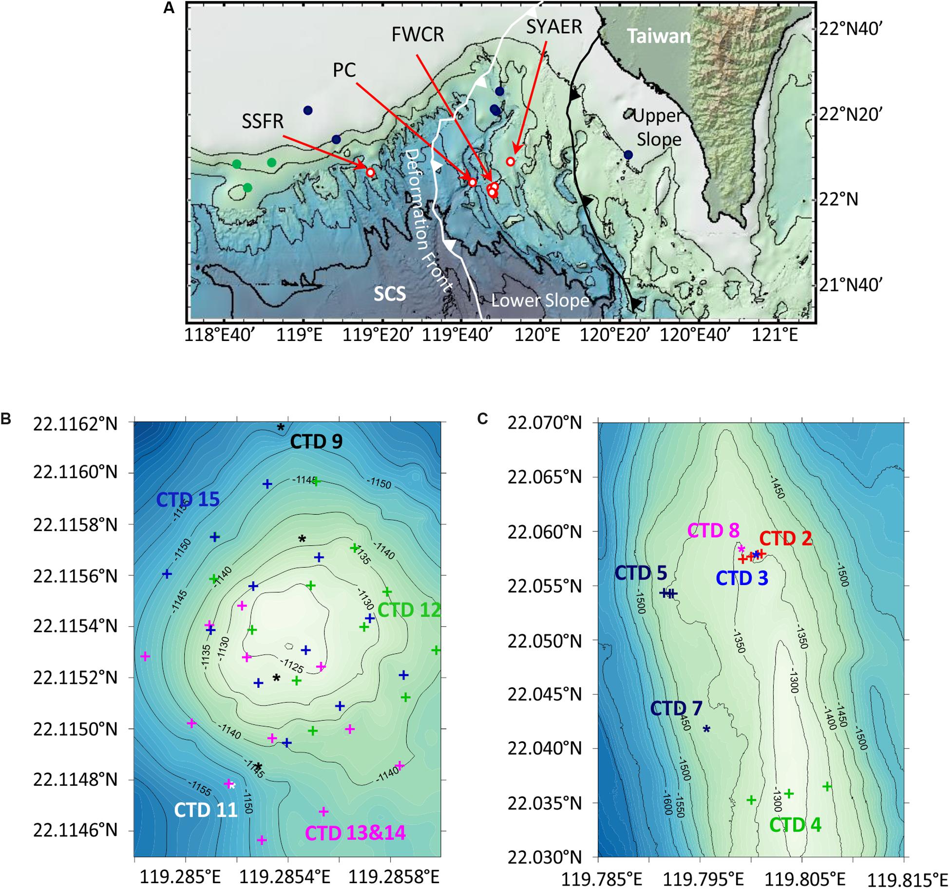
Figure 1. Maps of research areas SW of Taiwan. (A) Overview map of the northern South China Sea (SCS) including water column sampling stations at Southern Summit Formosa Ridge (SSFR), Penyu Canyon (PC), Four Way Closure Ridge (FWCR), and South Yun An East Ridge (SYAER), which are all shown as red circles. Stations, where the water column was sampled for methane concentration analyses by Yang et al. (2006) are displayed as dark blue dots, and stations where authigenic carbonates were observed by Han et al. (2008) are shown as green dots. The deformation front (white line) and the upper and lower slope boundary (black line) are adopted from Lin et al. (2009). (B,C) Bathymetric maps of SSFR and FWCR that include locations of CTD-hydrocasts.
The water column surveys also revealed methane concentrations above atmospheric equilibrium values in the surface water (Chen and Tseng, 2006; Yang et al., 2006; Zhou et al., 2009; Tseng et al., 2017) from July to September, when all the cruises took place, i.e., at the end of the summer monsoon and the beginning of the winter monsoon. Methane concentrations were higher above the continental shelf than over the deep ocean and did not correlate with chlorophyll a (Tseng et al., 2017). The latter result suggests no direct link between methanogenesis in the water column and phytoplankton biomass or photosynthesis, as has been proposed by Zindler et al. (2013) and Bogard et al. (2014).
In order to further explore the sources of the reported elevated methane concentrations, we participated on research cruise SO266 offshore SW Taiwan from 15th October to 18th November, i.e., during the winter monsoon. One of our aims was to detect seep sites at the active and passive continental margin and compare their activities with each other. The second aim was to investigate methane enrichments in the surface and subsurface water column that are not associated with seep sites. By correlating dissolved methane concentrations with aerobic microbial methane oxidation rates (MOxs), microbial community composition, oceanographic and hydroacoustic data we intended to reveal potentially important links for studies of the ocean methane paradox. Finally, we tested how coring by gravity corer and by MeBo-Drilling affected methane discharge and microbial consumption.
Materials and Methods
Water Sampling
We collected water samples at three different ridges and in a canyon during cruise SO266. We studied most extensively the Four Way Closure Ridge (FWCR, Figures 1A,C) at the active continental margin and the Formosa Ridge (SSFR, Figures 1A,B) at the passive continental margin as signs of gas seepage in form of carbonate patches and hydroacoustically detected flares were observed (Bohrmann and SO266 Shipboard Participants, 2019). At FWCR water was sampled crossing two different carbonate patches (CTD-2 and CTD-5) and the southern part of a ridge (CTD-4) where gas emissions were hydroacoustically detected (Figure 1C; Bohrmann and SO266 Shipboard Participants, 2019). We collected water by lowering the CTD-water sampler to the seafloor and by raising the instrument to 30 m above the seafloor while taking samples every 5 m, then towing the CTD-water sampler to another position, lowering it again and so on. The acoustic positioning system POSIDONIA, which we clamped into the wire 27 m above the rosette, facilitated to sample water above targeted sites. In addition, water samples throughout the entire water column were collected at two different sites (CTD-3, CTD-7) as well as 1 h after taking a gravity core (CTD-3) and 3 h after a gas emission triggered by MeBo drilling a gas pocket (CTD-8). At the SSFR (Figure 1B) first a towed hydrocast was deployed crossing the carbonate patch, which covered the morphological height of the ridge and where active bubble emissions were detected (CTD-9) (Bohrmann and SO266 Shipboard Participants, 2019). Next a vertical profile through the water column was sampled (CTD-11) and then water was collected at 12 sites using a 4 × 3 point grid that covered the entire carbonate patch (CTD-12). At these 12 sites, we sampled water at 5 m and 10 m above the seafloor. The grid was extended toward the south (CTD-13 and CTD-14) and finally the same 12 sites as sampled during CTD-12 were repeatedly sampled (CTD-15). In addition to these two main seepage sites, FWCR and SSFR, a vertical profile through the water column was also investigated at South Yun An East Ridge (SYAER, CTD-6) at the active continental margin and in the Penghu Canyon (PC, CTD-10, Figure 1A).
Oceanographic Data
A Seabird CTD Model 911plus recorded oceanographic data. The CTD comprised conductivity, temperature, and pressure sensors as well as a SBE 43 oxygen sensor and a WET labs ECO FLNTURTD fluorometer. According to the manufacturers, the accuracy of the conductivity, temperature, pressure, and oxygen was ±0.0003 S m–1, ±0.0002°C, ±0.02%, and ±2% of saturation, respectively. The difference between the two salinity and temperature sensors were 0.0069 and 0.0010°C, respectively. The WETLabs FLNTU measured chlorophyll fluorescence (ChlF, λ excitation = 470 nm, λ emission = 695 nm) with a sensitivity of 0.025 μg l–1. The data are archived in PANGAEA (doi: 10.1594/PANGAEA.915954 and doi: 10.1594/PANGAEA.915990).
Methane Concentration
Methane concentrations of discrete water samples were analyzed using the batch mode of a Greenhouse Gas Analyzer (GGA, Los Gatos Research) following the procedure described by Geprägs (2016). Briefly, water was sampled directly from the Niskin bottles. Two 140 ml syringes were flushed and filled each with 100 ml of seawater avoiding any air bubbles. To each of the syringes, 40 ml of synthetic air without any methane were added. The syringes were shaken vigorously for over 1.5 minutes to allow for equilibration between water and headspace. The 40 ml headspace gas of each of the two syringes was transferred in a dry 140 ml syringe via a Luer Lock adapter and injected in the GGA. The transfer is essential to minimize the risk of water injection into the GGA. Right after the injection of the 80 ml headspace gas (40 ml of each of the sampled syringes), additional 60 ml of Zero Air were injected, as needed to reach the required volume of 140 ml of the analyzing chamber of the GGA. The reproducibility of the method is <2.5%. Processing of 24 samples from the Niskin bottles took about 2 h.
Methane concentrations in atmospheric equilibrium was derived using the mean atmospheric methane concentration of Dongsha Island in October/November 2018 (1.983 ppm)1, the Bunsen solubility given by Wiesenburg and Guinasso (1979) and measured ocean temperatures and salinities.
Aerobic Methane Oxidation Rates
Methane oxidation rate (MOx) measurements were implemented as described by Mau et al. (2013) and Bussmann et al. (2015). Briefly, water was sampled in 100 ml crimp-top sample bottles. First, 25% sulfuric acid (0.3 ml) was added to control samples stopping microbial metabolism. Then, in the case of common measurements of MOxs, [3H]-CH4 in N2 (50 μl, 20.000 DPM) was added to each sample bottles by syringe whereupon displaced water can pass off through an additional needle. All bottles were subsequently shaken to equilibrate the tracer with the liquid phase. After that, the sample bottles were incubated for 24 h in the dark at 3, 10, 20, or 25°C (± 3°C) as close as possible to the in situ temperatures ranging from 3 to 27°C. At the end of the incubation period, a 1 ml aliquot of each sample was taken and mixed with 5 ml Ultima Gold scintillation cocktail for analysis in a liquid scintillation counter (Perkin Elmer Tri-Carb, 2910) on board to determine the total radioactivity injected. Finally, the sample was sparged for ≥ 30 min with helium to remove remaining [3H]-CH4 and a 1 ml aliquot was analyzed again by wet scintillation counting.
Furthermore, time series and temperature incubations were conducted to investigate possible differences between the methanotrophic communities in different water depth. Therefore, surface water (30 m), intermediate water (400 m) and deep water above carbonate patches of FWCR and SSFR was collected and incubated for 1–5 days in case of the time series and at four different temperatures (3, 10, 20, and 25°C) in case of the temperature evaluation. Always a duplicate sample and a control sample, which was treated with 0.3 ml of 25% H2SO4, was incubated for either a certain time period or at a certain temperature. The incubations were terminated as described above.
MOx-rates were calculated assuming first-order kinetics (Reeburgh et al., 1991; Valentine et al., 2001):
where k’ is the effective first-order rate constant calculated as the fraction of labeled methane oxidized per unit time, and [CH4] is the in situ methane concentration. The rate constant k’ provides an indication of the relative activity of methane oxidizing microorganisms in a water sample (Koschel, 1980) and is a first order rate constant if the reaction is solely dependent on methane concentration and biomass does not increase during incubation. Time series incubation show constant values of k’ over a period of 3 days confirming a first order reaction until then. Methane concentration and aerobic MOx data are archived in PANGAEA (doi: 10.1594/PANGAEA.916201).
Acoustic Doppler Current Profiler Data
An on-board Acoustic Doppler Current Profiler (ADCP, Teledyne RDI Ocean Surveyor, 38 kHz) was used to measure vertical profiles of water current velocity. The vertical resolution was set to 16 m depth cell (bins) with an average sampling interval of 12 s (ensembles). Simultaneous deployment with the other hydroacoustic devices caused typical interference patterns, visible in the echo intensity profiles of each beam. Therefore, raw beam velocities were screened and marked bad referring to corresponding peaks in echo intensity before further calculations. Beam coordinates were transformed to earth coordinates using gyro and heading information from external ship sensors. The moving platform correction was based on ADCP bottom track velocities. To determine one current velocity profile, all ensembles collected during the time of one CTD cast were combined (ca. 1.5 h, 450 ensembles) by first averaging independent velocity components and then calculating magnitude and direction. This reduced the error of measured current velocity in a specific depth to less than 3 cm s–1.
Hydroacoustic Profiling
Bathymetric data were recorded with the EM122 multibeam echosounder (MBES) operating at a frequency of 12 kHz. The software package MB-System Version 5.5.2213 and 5.5.2289 (Caress and Chayes, 1995) was used for bathymetric post-processing. After converting the data, the records were corrected for SVP and tides. Then, the data were manually edited, processed, and final grids were made.
Water column data (WCD) were recorded using the same MBES. We investigated the data to identify features of dense concentrations of particles and/or plankton to correlate those with measured methane concentrations. The software package QPS Fledermaus was used to convert the raw WCD into.gwc files, which later were visualized in the same tool for investigations and interpretation.
Flux Estimation
In order to derive the flux of methane from the ground into the ocean at the two seepage sites FWCR and SSFR, we calculated the amount of methane above the seepage sites and how long it takes to replenish this methane as it is constantly carried away by ocean currents. This flux estimation excludes any methane that remained in emitted bubbles from the seafloor.
We first estimated the inventory of methane (I in unit mol) within a box defined by the locations of the hydrocasts. We used the more accurate POSIDONIA positions instead of the ship position to calculate surface areas and volumes of these imagined boxes. For example, we collected water samples in a grid like fashion covering an area of ∼100 × 110 m above SSFR. The corner points of the grid defined the surveyed area and the sampling at ∼5 and 10 m above the seafloor defined the height of the box, i.e., ∼5 m. As the seafloor was uneven due to the carbonate mound, we used the software Surfer to generate a grid based on the lowermost water samples and another grid for the uppermost water samples and used the function volume to derive the volume between these two layers. This volume multiplied with the average methane anomalies, within the box according to Simpson’s law gives the inventory of methane above the seep site. Hence, we averaged the methane concentrations of the 12 grid point at 5 m and the 12 grid points at 10 m distance to the seafloor for SSFR and subtracted equilibrium methane concentrations according to temperature and salinity of the seawater (Wiesenburg and Guinasso, 1979). As we sampled the grid three times, we derived the inventory for each sampled 2-layer-grid. For FWCR we used data of hydrocasts CTD 2, CTD 4, and CTD 5 to define the volume and average of methane concentrations. The transects sampled during these hyrocasts crossed two carbonate patches and the southern FWCR from ca. 5 to ∼30 m above the seafloor. As we found similar methane concentration in the entire area, we summarized those transects to one large box.
Next, we calculated the output (R) in units of mol s–1. For this, we multiplied the inventory (I) with current velocity [u(z)] and divided the result by the lengths of the path it would take to move the entire box away from its original position (lpath).
The current direction and the surface area of the box define the lengths of the path, which we measured assuming parallel flow of water above ground by using the software Surfer. Current velocities and directions, recorded by ADCP in the appropriate depth where water was sampled, were used for the estimation.
Finally, we divided the output by the surface area of the grid (A) to derive the flux from the ground into the water column (F).
The uncertainty of the estimated flux is mainly due to the error of the current data; therefore, we included the range of current velocities and directions as shown in Table 1.
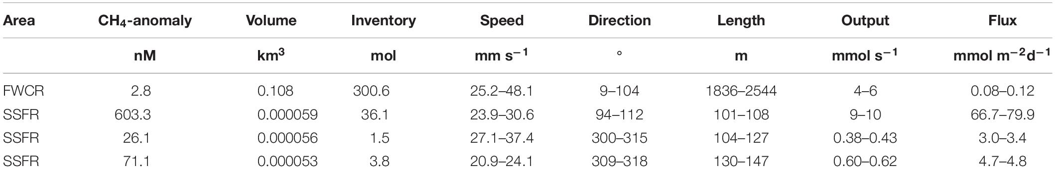
Table 1. Estimation of methane flux from the seafloor at two seep sites FWCR and SSFR based on methane anomaly (equilibrium methane concentrations subtracted from measured methane concentrations) and current speed and direction.
Characterization of the Microbial Community
Nucleic Acid Extraction and Sequencing
Water samples for the extraction of nucleic acid was filtered onto 0.2 μm Supor-200 (Pall Gelman) 47 mm filters at a rate of approximately 100 ml min–1, preserved in LifeGuardTM soil preservation solution (Qiagen, Germany), and immediately stored at −80°C. In order to prevent repeatedly melting and freezing samples, the extraction of DNA and RNA was completed in the same day. We extracted DNA and RNA from filtered water samples using the DNeasy Powersoil kit (Qiagen, Germany) and Quick-RNA Fecal/Soil Microbe Microprep Kit (Zymo, United States), respectively (volume of filtered water listed in Supplementary Table S1). In total, crude DNA and RNA was extracted from 23 and 17 samples, respectively. cDNA was synthesized immediately following the extraction of RNA using a SuperScriptTM IV VILOtTM Master Mix with ezDNasetTM Enzyme (Invitrogen, United States). The quantification of nucleic acid was implemented using QuantiFluor® dsDNA, ssDNA and RNA Systems (Promega, United States). Extracted and synthesized nucleic acid were stored at −80°C for subsequent analysis.
High-throughput sequencing of dual-indexed PCR amplicons encompassing the V4 region of 16S rRNA gene and partial sequence of particulate methane monooxygenase gene (pmoA) were conducted to assess the whole and aerobic methanotrophic community compositions in all samples, respectively. Fragments of 16S rRNA genes were amplified using the primer combination of F515 (5′–GTGCCAGCMGCCGCGGTAA–3′) and R806 (5′–CCCGTCAATTCMTTTRAGT–3′) that target both bacterial and archaeal communities (Kozich et al., 2013). Both forward and reverse primers were barcoded and appended with the Illumina-specific adapters. Each PCR mixture contained 1.1–1.5 ng of purified genomic DNA, 1U of ExTaq polymerase (TaKaRa Bio, Japan), 0.2 mM of dNTPs, 0.2 μM of each primer, and 2.5 μl of 10 × PCR buffer in a total volume of 25 μl. Thermal cycling involved a denaturation step at 94°C for 3 min followed by 30 cycles of denaturation at 94°C for 45 s, annealing at 55°C for 45 s, extension at 72°C for 90 s, and a final extension step at 72°C for 10 min. Amplification of pmoA was performed with a two-step PCR approach using primer combinations of pmoA189f (5′–GGNGACTGGGACTTCTGG–3′) and pmoA 661r (5′–CCGGMGCAACGTCYTTACC–3′) (Kolb et al., 2003). The reagents for PCR were the same as those for 16S rRNA. Nested PCR was performed to avoid the potential variations in efficiency of multiplexing PCR. For the first PCR, the thermal cycling was conducted with a denaturation step at 94°C for 3 min followed by 40 cycles of denaturation at 94°C for 45 s, annealing at 56°C for 45 s, extension at 72°C for 90 s, and a final extension step at 72°C for 10 min. The target region of pmoA were successfully amplified for 13 samples from CTD-2, 4, 6, 7, 9, and 10 (Supplementary Table S1). The amplicons from three independent PCRs for individual samples were pooled and purified as described in Tu et al. (2017), and subsequently used as templates in the second PCR, in which 10 cycles of amplification were performed with barcoded primers under the scheme of thermal cycling same as that for the first PCR. Regardless of genes, amplicons from different samples were pooled in equal quantities sufficient for sequencing on an Illumina Miseq platform (Illumina, United States).
Quantitative PCR Analysis
Quantitative PCR (qPCR) and quantitative reverse transcription PCR (qRT-PCR) were used to analyze the copy number and gene expression at transcriptional level of 16S rRNA genes for bacteria and pmoA for aerobic methanotrophs in all DNA and cDNA extracts using a QuantStudio 3 real-time PCR systems (Thermo Fisher Scientific, United States). All samples were analyzed in triplicate reactions (20 μl each) with each composed of 1 x SYBR green PCR master mix (Thermo Fisher Scientific, United States), 200 nM of each primer, and 2 μl of template DNA/cDNA. Primers targeting specific groups included: B27f and EUB338r for bacteria (Lipp et al., 2008) and pmoA189f and pmoA661r for aerobic methanotrophs. Each qPCR temperature program started at 95°C for 10 min, followed by 40 cycles of 15 s denaturation at 95°C and 1 min annealing. The annealing temperatures were: 56°C for bacteria and 59°C for aerobic methanotrophs. Primer specificity was confirmed by both melting curve analysis and gel electrophoresis. Standard preparations were the same as those described in Tu et al. (2017) and Lin et al. (2018). The copy numbers of genes represented the average of three measurements and were calculated with the length of amplicon, assuming 650 g mol–1 of one base pair of DNA. The quantity of pmoA genes was normalized to the abundance of 16S rRNA genes.
Sequence Processing and Analysis of 16S rRNA Gene and pmoA Amplicon
Sequences of 16S rRNA amplicons were analyzed using Mothur 1.42.3 following the standard protocols described by Schloss et al. (2009). Unique reads were aligned to the Silva SSU database of the NR 132 release2. Reads not aligned in the same region were removed. Sequence regions beyond the primers were truncated. Potential chimeric sequences were detected and removed using the UCHIME program (Edgar et al., 2011). The obtained sequences were deposited in GenBank under the Bio-project accession number: PRJNA592351. The number of sequences in each sample after quality filtering is shown in Supplementary Table S1. The assignment of taxonomic information to each read is based on the NR 132 release following the procedures described in Tu et al. (2017).
The usearch command “fastq_mergepairs” from UPARSE (Edgar, 2013) was used to assemble pmoA reads from the Illumina amplicon sequencing. The assembled reads were filtered using the usearch command “fastq_filter” to remove sequences shorter than 150 bp and with expected errors larger than 0.5. The remaining reads were denoised by the usearch command “unoise3” to identify and correct sequencing errors as well as to remove chimera and reads with abundance lower than 4. The built-in UNOISE algorithm generated zero-radius OTUs (ZOTUs) to report all correct biological sequences in the reads. The representative sequences of ZOTUs were subsequently analyzed using the FunGene Pipeline Version 9.8 (Fish et al., 2013). Based on the reference sequences of pmoA, reads were translated into amino acids by FrameBot (Wang et al., 2013). The translated sequences shorter than 50 a.a., possessing frameshift errors and inframe STOP codons were removed. The number of sequences in each sample after quality filtering is shown in Supplementary Table S1. Subsequently, the remaining high quality sequences were clustered at 93% similarity (threshold for genus level) (Degelmann et al., 2010; Bragina et al., 2013). The amino acid sequences of six representative pmoA OTUs were aligned with 129 reference pmoA sequences retrieved from FunGene database (Kalign, default parameters, Madeira et al., 2019). The phylogenetic tree was reconstructed using the Simply Phylogeny tool (default setting, Madeira et al., 2019) based on Neighbor-joining algorism. The type II pmoA sequences were used to root the phylogenetic tree.
All statistical analyses and visualization were performed in the R software (Version 3.6.1, R Development Core Team, 2013, 2017) using phyloseq (McMurdie and Holmes, 2013), vegan (Dixon, 2003), metagenomeSeq (Paulson et al., 2013), and ggplot2 (Wickham, 2016) packages. Pearsons’s correlations were calculated using ggplot2 to test whether the transcription of pmoA correlated with the concentration of methane and the rate of methane oxidation.
Results
Oceanographic Data
The water column in the northern SCS can be separated into depth zones with distinct characteristics (Figure 2). The mixed layer reached down to 50 m. The water of this zone had a temperature of 27–28°C and salinities between 33.7 and 34.4 (Figures 2A,B). Temperature refers throughout the text to potential temperature, i.e., the temperature a water parcel has when it is brought to the surface to exclude the effect of pressure resulting in warmer water. The oxygen concentrations range between 4.2 and 4.4 ml l–1 (Figure 2D). In the thermocline beneath the mixed layer, the temperatures dropped from 28 to 12°C from 50 to 300 m water depth, respectively. In this zone several other features occurred. Fluorescence peaked between 50 and 125 m in the upper thermocline (Figure 2E) and a salinity maximum was centered at ∼150 m. Beneath the thermocline, salinity decreased to 34.4 at 300–650 m and the oxycline extended to ∼800 m where oxygen concentrations were as low as 1.9 ml/l. In the deep water below 1000 m, salinity increased to 34.6, oxygen concentrations increased to 2.4 ml l–1, and temperature decreased to 2°C at 2000 m.
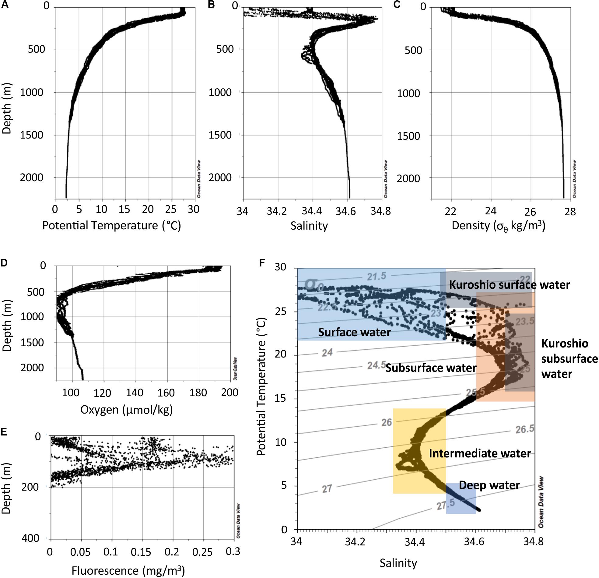
Figure 2. Depth profiles of all measurements of potential temperature (A), salinity (B), potential density (σθ) derived from potential temperature and in situ salinity (C), oxygen concentration (D), and fluorescence (E). (F) Potential temperature versus salinity data of all stations. The colored rectangles indicate potential temperatures and salinities of local water masses as described in Hu et al. (2011).
Apart from that vertical zonation, the research sites showed differences. In the mixed layer, water above FWCR was less saline than water above SSFR (Figure 3). Fluorescence peaked in the uppermost 50–100 m above FWCR and slightly deeper at 62–106 m above SSFR (Figure 3).
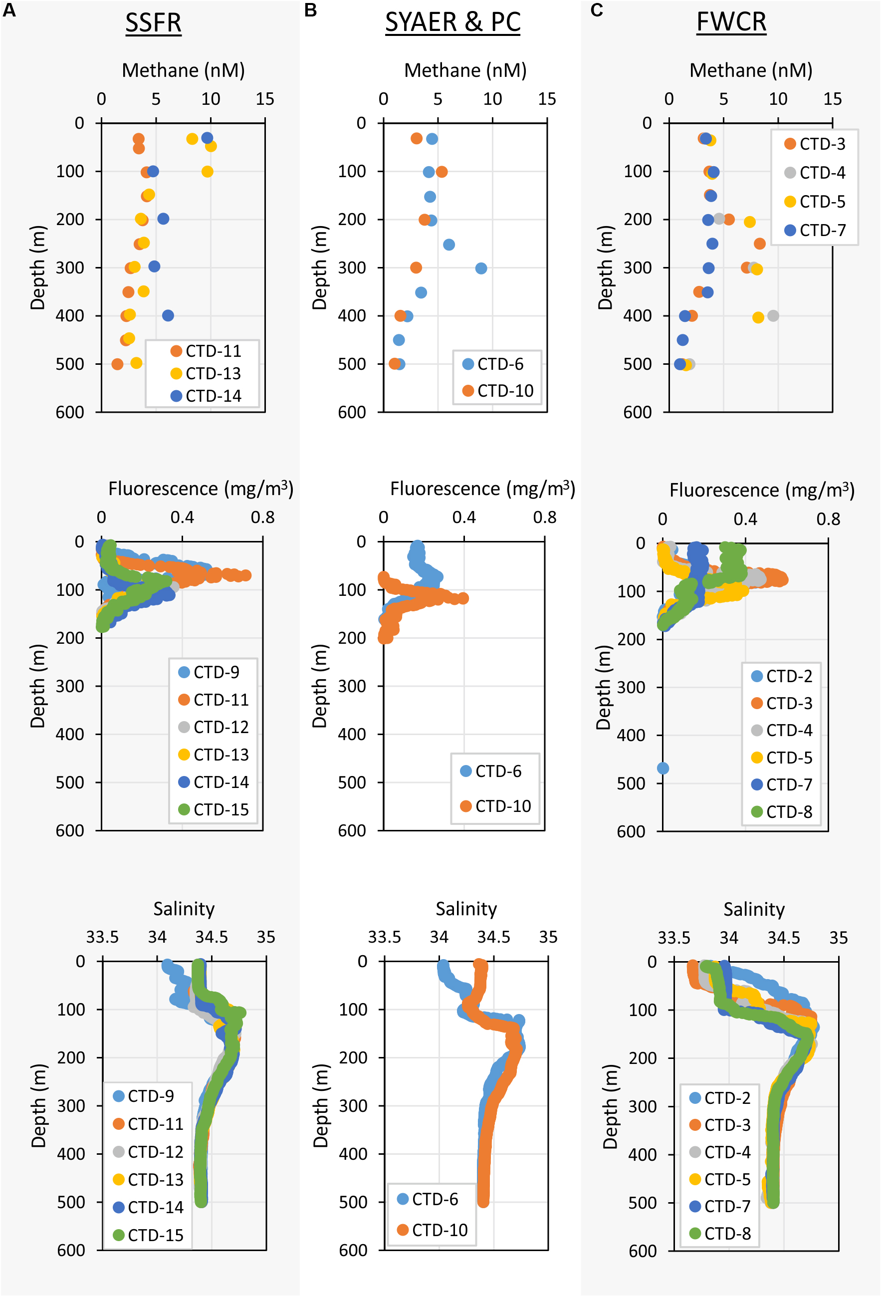
Figure 3. Depth profiles of methane concentrations – upper row, fluorescence – middle row, and salinity – lower row of the uppermost 500 m. (A) Shows the measurements of stations at SSFR – Southern Summit Formosa Ridge, (B) displays station data of SYAER – South Yun An East Ridge (CTD-6) and PC – Penghu Canyon (CTD-10), and (C) shows data recorded above FWCR – Four Way Closure Ridge.
Methane
Methane concentrations in atmospheric equilibrium would vary from 2.1 to 3.7 nM from sea surface to 2000 m. Elevated methane concentrations above these equilibrium concentrations indicate a source of methane apart from the atmosphere. Water from sea surface to 400 m and above seep sites below 1000 m contained such elevated methane concentrations (Figure 4A). Concentrations of 3–10 nM occurred in the uppermost 100 m above SSFR and between 200 and 400 m above FWCR and SYAER (Figure 3). In waters > 1000 m, we found increased methane concentrations above FWCR and SSFR, both areas of active bubble seepage as observed during cruise SO266 (Bohrmann and SO266 Shipboard Participants, 2019). However, methane concentrations did not exceed 10 nM at FWCR while reaching > 1000 nM above SSFR. Crossing two carbonate patches at the northern part of FWCR (CTD-2 and 5), methane concentrations were generally above 5 nM with increased concentrations at the edge of the larger and apparently more active carbonate patch (CTD-2; Figures 5A,B). Crossing the southern FWCR showed generally elevated methane concentrations of 5–8 nM (CTD-4; Figure 5C). Even at a site > 1 km away from the carbonate patches and any flare site, methane concentrations were slightly elevated (4.0–4.8 nM, CTD-7; Figure 5D). Overall, all stations in the area of FWCR showed increased methane concentrations.
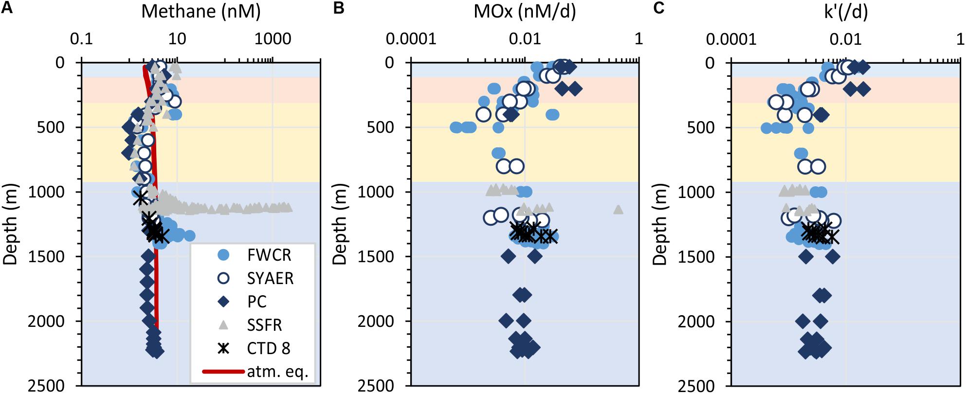
Figure 4. Depth profiles of methane concentrations (A), aerobic methane oxidation rates (B), and the relative activity of methanotrophic microorganisms – k’ (C). Horizontal colors refer to the water masses: surface water – blue, subsurface water – orange, intermediate water – yellow, and deep water – dark blue. The red line in (A) indicates the methane concentration in atmospheric equilibrium, i.e., values greater than the equilibrium concentrations suggest a source of methane. Symbols refer to the different sampling areas. Station CTD-8 located at FWCR was excluded, because these results display the difference, which results from sampling after a gas emission was caused by seabed drilling and the drilling rig was retrieved.
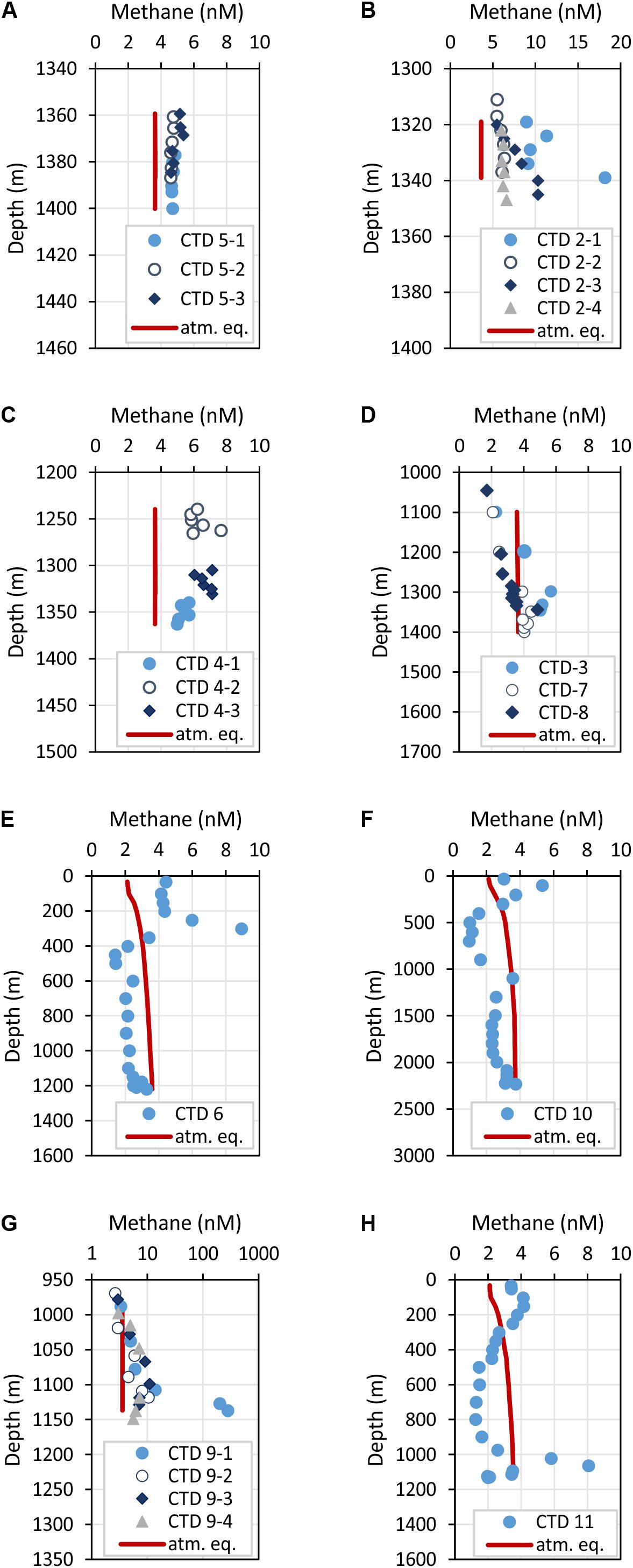
Figure 5. Depth profiles of methane concentrations crossing two carbonate patches at FWCR (A,B) and the southern part of FWCR (C). These data were used for methane flux estimation. Additional methane concentrations of water collected above FWCR are shown in (D). CTD-7 was indented to sample the background at FWCR, CTD-3 was taken after collecting a gravity core and CTD-8 after gas emission was caused by Mebo-drilling and subsequent retrieval of the seabed drilling rig. Methane concentrations above SYAER and PC are shown in (E,F), respectively. (G,H) Show methane concentrations of water sampled above SSFR; water was collected crossing the carbonate mound with hydrocast CTD-9 (G) and at the southern rim with hydrocast CTD-11 (H). The red lines mark the methane concentration in atmospheric equilibrium; values greater than the equilibrium concentrations indicate a source of methane. Note, the scale of methane concentrations in (B,G) vary to the common scale from 0 to 10 nM.
In contrast to the general moderate methane concentrations in the kilometer wide study area at FWCR, methane concentrations in the water above SSFR showed distinct peaks in the area of the carbonate paved morphological height, which is ∼140 m elevated above the surrounding seafloor and a location where distinctive flares were detected in hydroacoustic data (Bohrmann and SO266 Shipboard Participants, 2019). A transect crossing the SSFR (CTD-9) and a station near the southern edge (CTD-11) of the carbonate peak confirmed methane seepage (Figures 5G,H). Highest methane concentrations of 282 nM occurred south of the carbonate peak ∼ 5 m above ground whereas methane plumes with lower concentrations (<10 nM), but up to 100–150 m above ground, were found over the northern part (Figure 5G). The peak of the methane plumes varies from 5 m above seafloor (lowermost water sample) in the south to 20–30 m in the north and even 70 m above the seafloor at the station near the southern edge (Figure 5H). In comparison, at FWCR elevated methane concentrations were solely found 20–25 m above ground.
In addition to the transect crossing the carbonate peak, three grid like surveys were completed covering the area of the carbonate peak (Figure 6). The grids confirmed active and strong seepage in the area. However, the methane concentration range varied considerably over time, but indicated a source at the western side of the peak. We found highest methane concentrations during the first survey ranging between 10 and 2100 nM (Figures 6A,B). The second survey was shifted to the south and showed methane concentrations between 2 and 448 nM 1.5 days after the first survey (Figures 6C,D). The last survey was implemented another half a day later and revealed methane concentrations between 3 and 968 nM (Figures 6E,F).
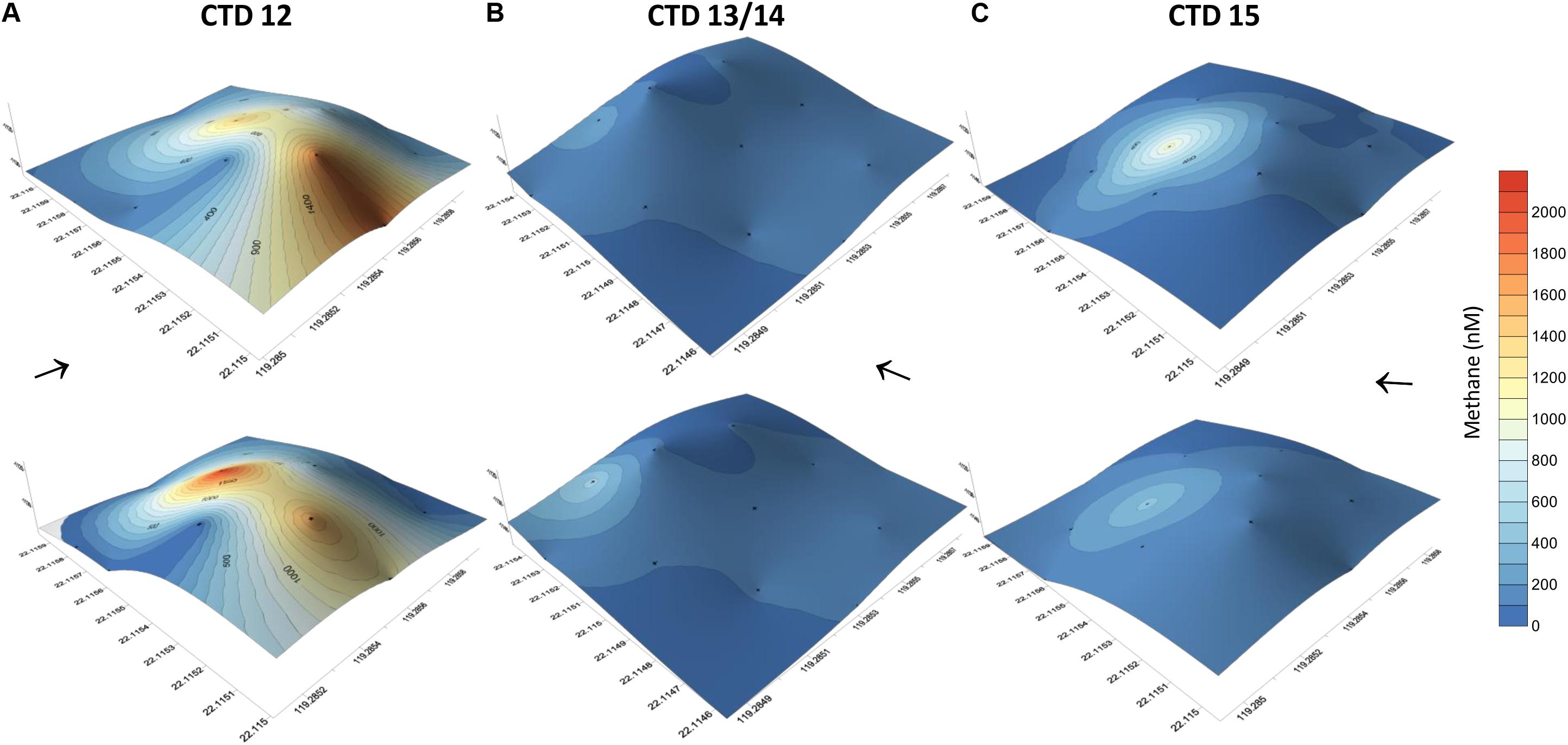
Figure 6. Methane concentrations of water collected at 12 sites using a 4 × 3 point grid that covered the entire carbonate patch at SSFR, see map Figure 1A. Methane concentrations are plotted on the topography of the mound. The grid was sampled first during hydrocast CTD-12 (A) and repeated after 1.5 day (CTD-13/14) (B). Another repetition was implemented after 0.5 days (CTD-15) (C). During the first repetition, the grid was moved to the SW (see Figure 1A). At the 12 sites, water was sampled at ∼5 m (lower row) and ∼10 m above the seafloor (upper row). Black arrows indicate current direction.
In contrast to these two seep sites, FWCR and SSFR, methane concentrations were below the equilibrium concentrations at SYAER (Figure 5E) and PC (Figure 5F). Although slightly elevated methane concentrations were observe near the seafloor at SYAER and at 1100 and 2230 m in the PC, the concentrations were still lower than methane equilibrium concentrations.
Besides, we tested if methane concentrations in the water column increase due to sediment sampling by gravity corer (CTD-3) and after a gas emission caused by MeBo-drilling at FWCR (CTD-8), but neither core sampling showed a methane concentrations greater than the ones already observed after 1 and 3 h, respectively (Figure 5D).
Aerobic Methane Oxidation Rates
Methane oxidation rates (MOx) range between 0.0006 and 0.44 nM d–1 with higher values in surface waters and waters above seep sites (Figure 4B). In the uppermost 400 m, a general increase of MOx and the relative activity (k’) of methane oxidizing microbes was observed toward the surface water yielding highest MOx and k’ in samples collected closest to the sea surface at ∼30 m water depth (Figures 4B,C). MOx-rates were elevated up to 0.076 nM d–1 in the uppermost 400 m, while k’ were increased up to 0.02 d–1 in the uppermost 200 m. We investigated surface water above FWCR and PC, but could not implement measurements above SSFR due to cruise time restrictions. Apart from the surface maxima, MOx-rates were elevated above seep sites. However, except from one value (0.43 nM d–1 above SSFR), MOx-rates were below 0.03 nM d–1 and thus lower than in the surface water (Figure 4B). In contrast, the relative activity k’ did not increase above 0.006 d–1 above seep sites and most data were even below 0.005 d–1 as in the waters above (400–1000 m) and below (in the PC, 1500–2200 m). Both MOx-rates and k’ were higher in the surface ocean than above seep sites.
MOx-rates and k’ were similar above the two seep-areas SSFR and FWCR. Comparing all data crossing the carbonate patches of FCWR and southern FWCR, MOx-rates were below 0.03 nM d–1 and k’-values were below 0.006 d–1. At SSFR, MOx-rates were also below 0.03 nM d–1 except of one value of 0.43 nM d–1 and k’ values were below 0.003 d–1. In order to test, if methanotrophic activity decreased with distance to the seafloor, we investigated MOx and k’ near the seafloor and 30 m above the seafloor at FWCR (crossing the carbonate patch, CTD-2), but found no difference. However, MOx and k’ were lower at 150 m above seafloor when compared to values at less than 10 m above ground at SSFR.
Time series incubations illustrated that the relative activity k’ of methane oxidizing microbes remained constant up to 3 days (Figure 7A). However, incubations of surface water showed an increase of k’ after 3 days while incubations of water from near the seafloor revealed a decrease of k’ after 3 days.
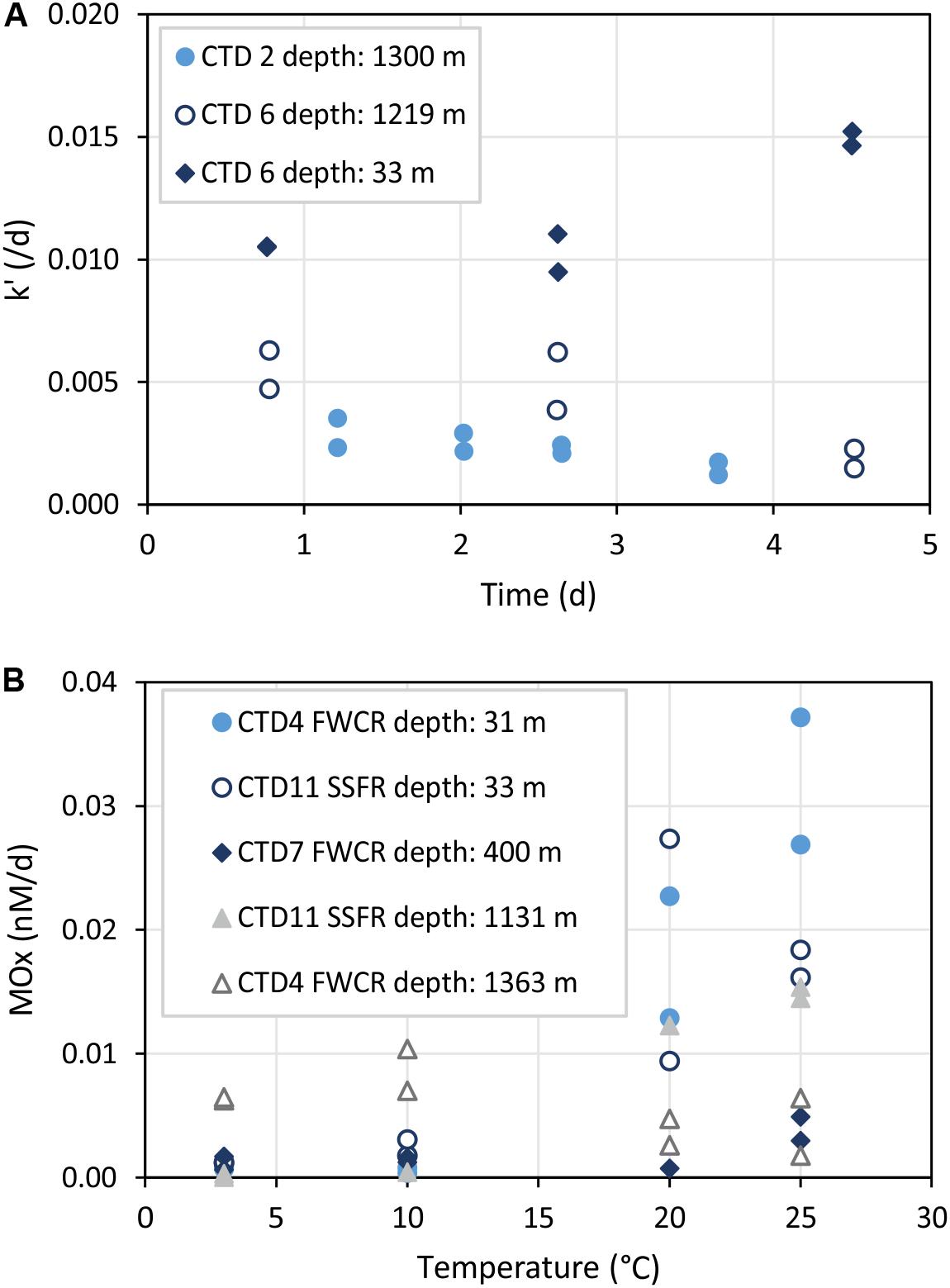
Figure 7. Time series (A) and temperature incubations (B) of water from different depths. k’ refers to the relative activity of methanotrophic microorganisms and MOx to the aerobic methane oxidation rate. (A) Shows that k’ remains constant up to 3 days. (B) Illustrates increased MOx at temperatures >20°C especially in surface water samples (CTD-4 FWCR depth: 31 m and CTD-11 SSFR depth: 33 m).
The influence of temperature on microbial methane oxidation was tested using surface water (∼30 m), intermediate water (400 m), and deep water above seep sites (>1000 m; Figure 7B). All except one set of incubations at different temperatures indicated increasing activity with increasing temperature. Samples of the one exception originated from 1363 m water depth collected above southern FWCR.
Investigations after gas emission caused by MeBo-drilling a gas-rich horizon, showed an elevated k’ in bottom water (MOx up to 0.0057 d–1, CTD-8, Figure 4). The other data were similar to measurements above the carbonate patches of the northern FWCR and seep sites at southern FWCR.
Current Speed and Direction
Currents shift considerably in space and time, but there are general differences between the eastern research area of FWCR and the western study site of SSFR (Figure 8). A northward component appeared to influence the general current pattern during the first week of sampling at FWCR (Figure 8C). In the uppermost 100 m of the water column at FWCR currents shifted from a strong northward (CTD2-3) to an eastward flow (CTD7-8). There also was a strong westward flow centered at 200 m, which turned from northwest (CTD2-3) to southwest (CTD7-8) over the course of 13 days. The northward influence diminished below ∼400 m, where waters mainly moved to the south. In contrast to this southern flow of intermediate and deep water above FWCR, northeast flow dominates almost the entire water column at the SSFR (Figure 8A), the western study site (CTD9, CTD11-15). PC situated between FWCR and SSFR, showed currents flowing toward the northeast down to 600 m (Figure 8B) similar to SSFR and water movement to the south below 600 m similar to FWCR. Surface currents at SYAER located farther to the east than FWCR moved eastward similar to the current flow at FWCR (Figure 8B), but the westward flow at 200 m was not observed as well as there was hardly any southward flow below 400 m.
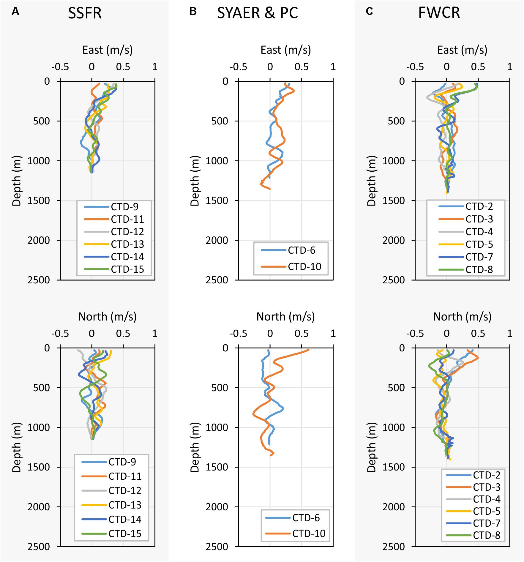
Figure 8. Depth profiles of the east (upper three graphs) and north velocities (lower three graphs). (A) Shows the east and north velocity of stations at SSFR – Southern Summit Formosa Ridge, (B) displays station data of SYAER – South Yun An East Ridge (CTD-6) and PC – Penghu Canyon (CTD-10), and (C) shows data recorded above FWCR – Four Way Closure Ridge.
Methane Output and Flux
Based on the measured methane concentrations and ADCP-records, we estimated the output in mmol s–1 and the flux of methane in mmol m–2 d–1 from the sediment into the water column ignoring any methane remaining in bubbles. We summarized data of three hydrocasts taken above FWCR (CTD-2, 4, 5; Figure 1C) for estimation and used the methane concentrations sampled in a grid-like fashion above SSFR, which was twice repeated. Due to the different sampling strategies, the volume of the imagined box including all methane concentration data above FWCR had a much larger volume of 108,939 × 103 m3 compared to the small scale grids sampled above SSFR with volumes of 59.8 × 10³ m3 for CTD-12, 56.5 × 10³ m3 for CTD-13/14, and 52.9 × 10³ m3 for CTD-15 (Table 1). The volumes above SSFR vary according to the actual positions of the water samples, which was recorded by POSIDONIA. The output was estimated to be 5 mmol s–1 for FWCR and varied between 9.5 mmol s–1 (CTD12), 0.4 mmol s–1 (CTD13/14), and 0.6 mmol s–1 (CTD15) above SSFR. Accordingly, fluxes yielded values between 0.08 and 0.12 mmol m–2 d–1 for FWCR and ranged between 67–80 mmol m–2 d–1 (CTD12), 3.0–3.4 mmol m–2 d–1 (CTD13/14), and 4.7–4.8 mmol m–2 d–1 (CTD15) during each of the three sampling periods above SSFR (Table 1).
Microbial Gene Abundance and Activity of Methanotrophs
Calibration for qPCR was well constrained with regression coefficients (R2 value) ranging between 0.996–0.997 and 0.993–0.996 for 16S rRNA and pmoA qPCR assays, respectively. The efficiencies of 16S rRNA and pmoA qPCR in all assays were between 86–95% and 80–91% allowing confident enumeration of 0.01 16S rRNA and 0.1 pmoA copies per milliliter of seawater in a 10 L sample, respectively.
The 16S rRNA and pmoA gene abundances along the water column (Figure 9) were measured above FWCR (CTD-2, 3, 8), the southern ridge of FWCR (SFWCR; CTD-4), and SSFR (CTD-11). Overall, gene abundances generated from most DNA and cDNA templates ranged between 0.5 and 70 copies of pmoA gene and between 0.3 and 26 copies of pmoA transcript per milliliter of seawater, respectively (Figure 9). The mean pmoA gene and transcript abundances were higher in the upper part than the rests of the water column with the highest value present in subsurface water collected above SFWCR (CTD-4, Figure 9B).
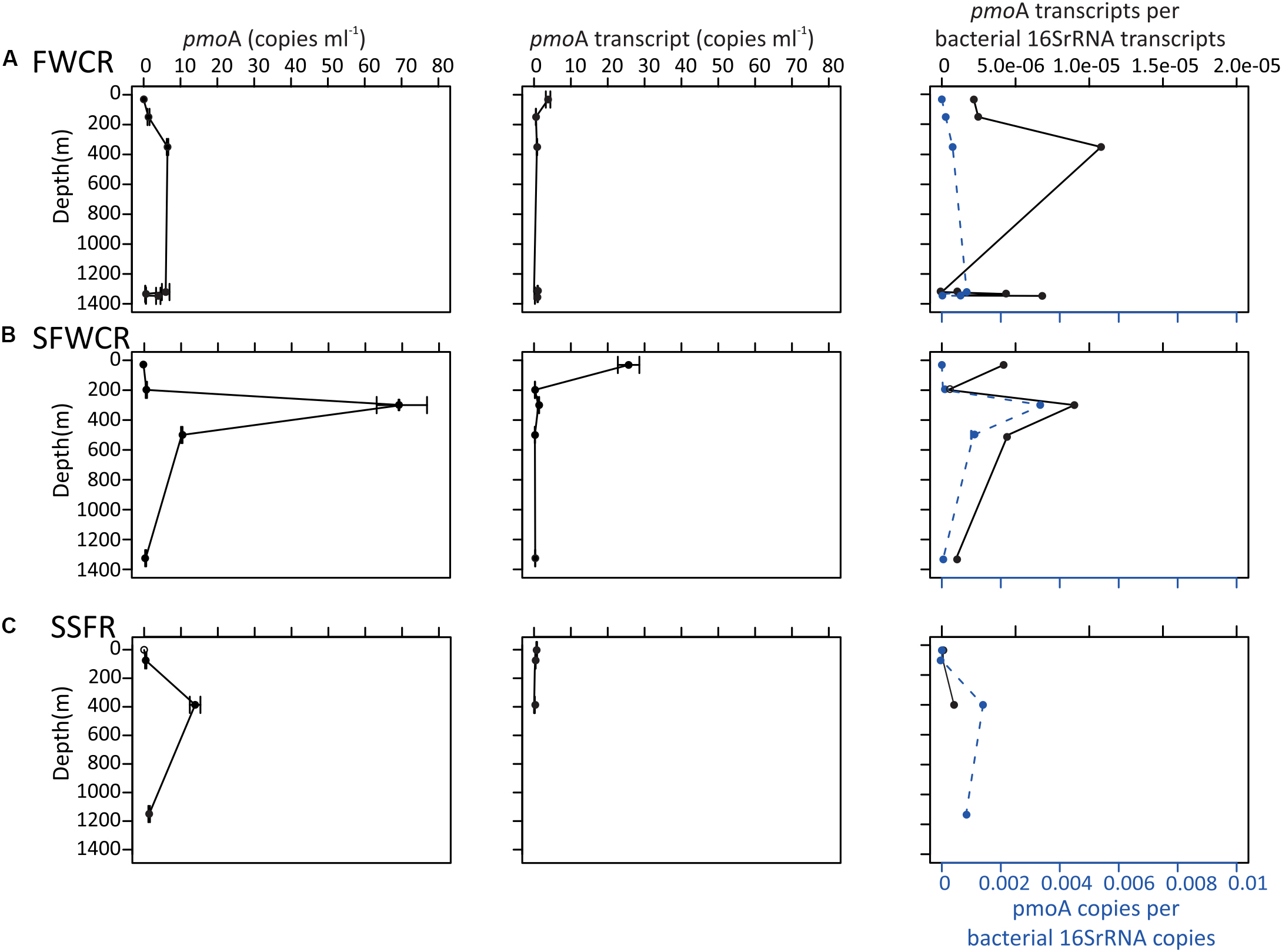
Figure 9. pmoA gene and transcript abundance in copies per milliliter of seawater, and the normalized pmoA gene to the abundance of 16S rRNA gene at the indicated depth above (A) FWCR, (B) SFWCR, and (C) SSFR. The number of copies and error bars represent the average and standard deviations calculated from four measurements.
The abundance ratio of pmoA genes to bacterial 16S rRNA genes ranged between 3.6 × 10⁻⁵ to 3.4 × 10⁻³ and was higher in samples collected above SFWCR than those above FWCR and SSFR. In contrast, the abundance ratio of transcripts between two genes ranged between 1.3 × 10⁻⁶ to 1.0 × 10⁻⁵ and was higher in water samples collected above FWCR than those above SFWCR and SSFR. These transcript ratios were lower than the average DNA ratio (Figure 9). In general, the highest transcript abundance ratios were present in the subsurface water in all hydrocasts. Although the transcript abundance of pmoA showed no clear trend with the in situ concentration of methane (Figure 10A), it demonstrated a strong correlation with the MOx and k’ value in FWCR (Figures 10B,C).
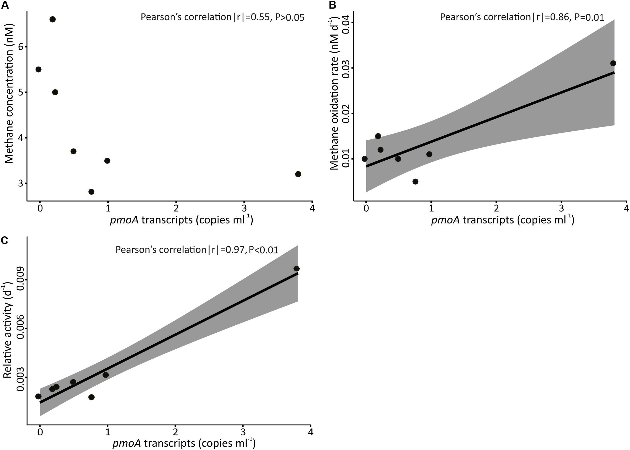
Figure 10. Concentration of pmoA transcripts in samples collected above FWCR against (A) concentration of methane, (B) methane oxidation rate, and (C) relative activity. The shading represents ± 95% confidence intervals.
Microbial Community Composition
A total of 1,344,605 16S rRNA reads and 78,096 pmoA reads were obtained after quality control and cleaning, and corresponded to a total of 63,571 OTUs at 97% similarity and six OTUs at 93% similarity, respectively. Based on 16S rRNA composition, the family Methylomonaceae within the order Methylococcales is the only detected aerobic methanotroph present in the water column. The fraction of Methylomonaceae varied along depth and among sampling sites, accounting for less than 0.1–5.7 and 14.7% of the total reads at DNA and cDNA levels, respectively (Figure 11). Except for the high fractions (5.7% for DNA and 14.7% for RNA reads) for samples collected after the MeBo drilling on a gas-rich horizon (CTD-8, 1241 m), the relative abundances of both DNA and cDNA sequences affiliated with the family Methylomonaceae showed a trend of increase from the surface to the bottom in hydrocasts CTD-3, CTD-4, and CTD-11 taken above FWCR and SSFR (Figure 11). Sequences assigned to the family Methylomonaceae could be further categorized into 8 clades including two genera with culture representatives, Methylomonas and Methyloprofundus as well as 6 uncultured clades (Figure 11). Among these clades, the clade IheB2-23 was the most abundant one at all depths, comprising from less than 0.01 to 8.2% (for the transcripts in sample collected after Mebo-drilling at FWCR) of the sequences. The remaining sequences of the family Methylomonaceae were mainly affiliated with the clade Milano-WF1B-03 (Figure 11).
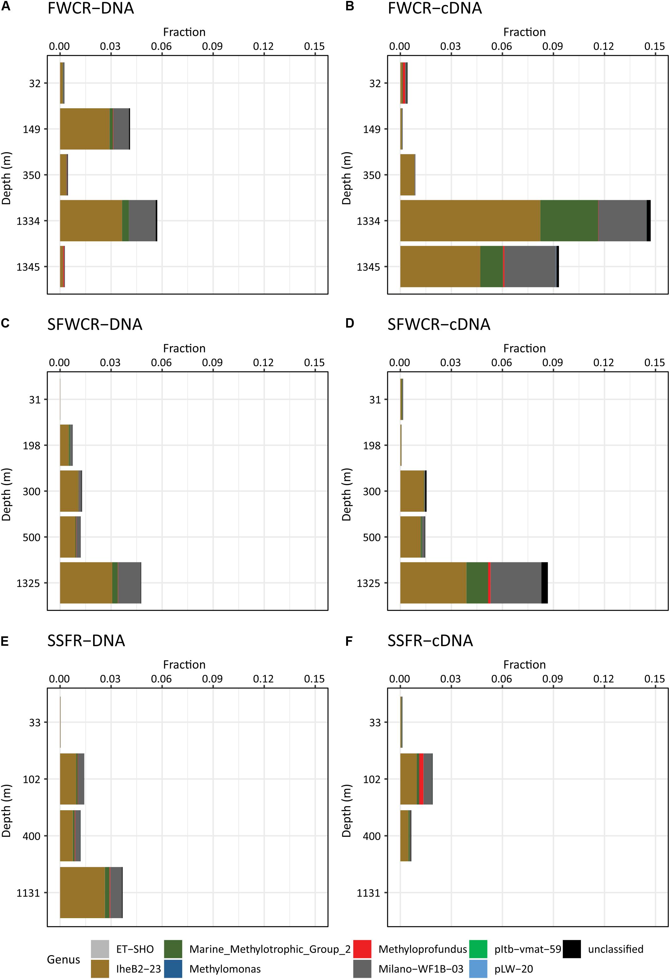
Figure 11. The relative abundance of methanotrophs in the water column based on 16S rRNA gene sequences (A) above FWCR at DNA level (B) above FWCR at cDNA level, (C) above SFWCR at DNA level, (D) above SFWCR at cDNA level, (E) above SSFR at DNA level, (F) above SSFR at cDNA level.
Phylogenetic analysis based on pmoA sequences showed that the most two dominant pmoA OTUs were affiliated with type Ia methanotrophs (pmoA OTU03) and type Ib methanotrophs (pmoA OTU06) (Figure 12A). The type Ia related pmoA OTU03 dominated over others in samples collected from >1000 m water depth (43.8–88.2% of the pmoA sequences in each sample) (Figure 12B). In contrast, the abundances of type Ib related pmoA OTU06 exceeded others in samples taken from 100 to 500 m water depth (98.7–99.6% of the total pmoA reads in each sample) (Figure 12B).
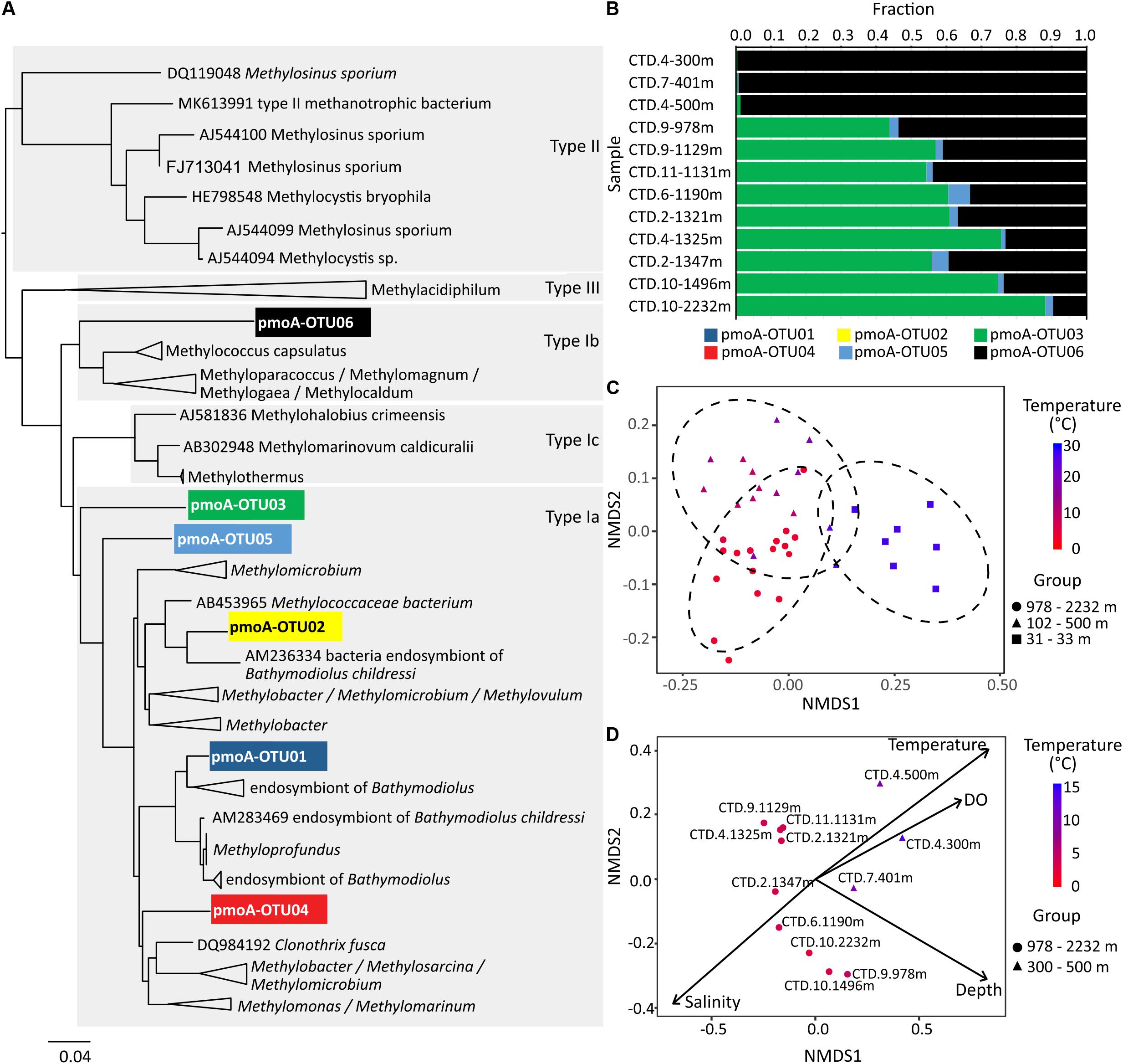
Figure 12. The N-J tree (A) and relative abundances (B) of pmoA OTUs in water samples. Non-metric multidimensional scaling plot of beta diversity based on 16S rRNA gene amplicons in (C) and pmoA gene amplicons in (D). In (C) the 95% confidence ellipses circumscribe the samples from different water depths, and in (D) vectors represent environmental variables that significantly correlated with the ordination space with length corresponding to the strength of the correlation.
Pairwise comparisons based on the 16S rRNA gene showed that the whole microbial community in samples from the upper region of the water column, i.e., 30 m water depth, were grouped together and separated from those from the middle (100–500 m) or bottom parts (>1000 m) of the water column (Figure 12C). Community similarities were significantly correlated with water temperature (R2 = 0.695), concentrations of dissolved oxygen (R2 = 0.681), and water depth (R2 = 0.543) in the NMDS ordination for 16S rRNA genes (both DNA and cDNA; P-value for all mentioned values ≤0.001; Supplementary Table S2). Likewise, the community similarities for pmoA genes inferred from the NMDS ordination were also significantly correlated with water temperature (R2 = 0.859, P≤ 0.001), water depth (R2 = 0.778, P ≤ 0.001), salinity (R2 = 0.619, P = 0.020), and dissolved oxygen (R2 = 0.553, P = 0.015) (Figure 12D and Supplementary Table S3).
Discussion
Methane Concentration and Microbial Oxidation in the Different Water Masses
The T-S-plot indicates four water masses, which have been described by Hu et al. (2011) (Figure 2F). The surface water extends from sea surface to ∼100 m and is characterized by low salinities (33.5–34.5). According to our results, this part contains the surface mixed water and the upper thermocline water. A salinity maximum (S > 34.6) marks the subsurface water, which is located at water depth between 100 and 200 m and includes the middle part of the thermocline. Beneath at 200–300 m, subsurface water mixes with intermediate water in the lower part of the thermocline. For simplicity, we merge these two depth zones and call it subsurface water. Below this depth zone, intermediate water with salinities of <34.5 extends from 300 to 900 m. Within this depth zone, the oxygen minimum zones is located. Finally, deep water with salinities between 34.5 and 34.6 fills the SCS in the investigated areas.
Seep derived methane affected solely the deep water mass whereas methane anomalies in the upper ocean were not restricted to one water mass. We found elevated methane concentrations in the surface water, the subsurface water, and in the upper part of the intermediate water (to 400 m) (Figure 4A). Microbial MOx-rates were similarly elevated in those water masses, but in contrast to the methane concentration, which were higher near the seafloor; MOx-rates were higher in the uppermost 400 m. These high MOx-rates in the uppermost 400 m resulted from high values of the relative activity (k’) of methane oxidizing microbes (Figures 4B,C). Based on these results, we termed the methane anomalies to be located in the upper water column (including surface, subsurface and intermediate water) and in the lower water column (in deep water).
In order to reveal the community composition and activity of methanotrophic bacteria, we observed that the pmoA gene abundance of methanotrophic community ranged between 0.5 and 70 copies per milliliter. Higher abundance occurred at 400 m (Figure 9), i.e., at the lower boundary of elevated methane concentration in the upper water column. In contrast, the number of pmoA transcripts was highest in the surface SCS (Figure 9) where MOx-rates and k’ values were increased. Pearson’s correlation confirmed a linear relationship between the transcripts of pmoA and both, MOx and k’, above FWCR (Figure 10). These results are similar to previous studies in a boreal wetland and rice paddy soils, highlighting the number of pmoA transcripts as a proxy of methanotrophic activity (Reim et al., 2012; Siljanen et al., 2012). In contrast to the positive correlation between pmoA transcript abundances and MOx and k’ values, a significant negative correlation between the number of pmoA transcripts and methane concentrations was revealed by excluding the point with the highest pmoA transcripts (Pearson’s correlation |r| = −0.82, P = 0.04), suggesting a net drawdown of methane concentration by elevated methanotrophic activities.
Temperature and Methanotrophy Relation
In the upper ocean, methane generation and consumption appears layered and closely related with temperature (Figure 13). Methane concentrations above the equilibrium concentration extended to a depth of 400 m. The increase in methane concentration correlated with temperatures >10°C (Figure 13A). In contrast, aerobic methanotrophic activities were mainly elevated in the uppermost 100 m correlating with temperatures >19°C (note no data in the region above SSFR; Figure 13B). MOx-rates determined from incubations of water samples at different temperatures (3, 10, 20, and 25°C) also suggest higher relative activity at temperatures >20°C in water samples collected in ∼30 m (Figure 7B). In conclusion, while methane generation appeared to take place in the uppermost 400 m, aerobic microbial methane consumption was restricted to predominantly the uppermost 100 m. Based on our data set, temperature appears to play an important role controlling microbial generation and consumption of methane in the study region.
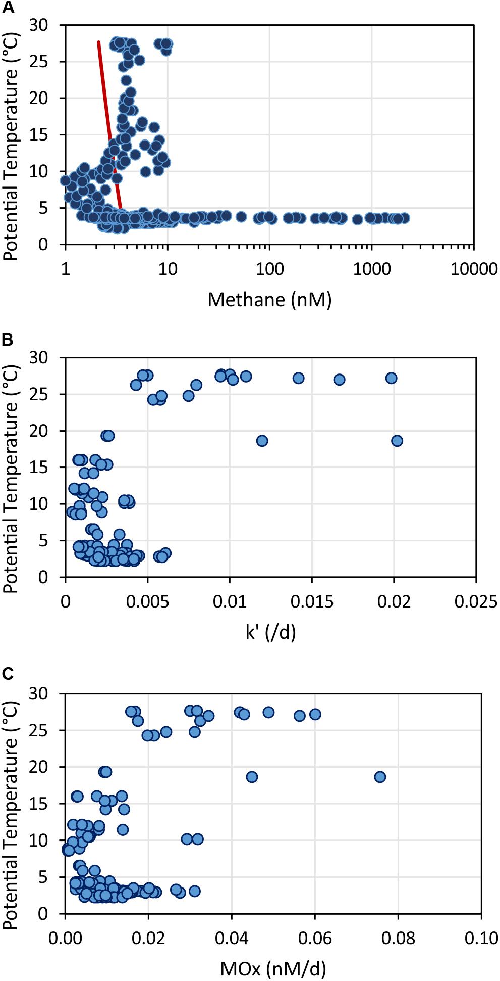
Figure 13. Methane concentrations (A), relative activities of methane oxidizing microbes – k’ (B), and aerobic methane oxidation rates – MOx (C) plotted against potential temperature. The red line in (A) shows the calculated methane concentration in atmospheric equilibrium. Values greater than the equilibrium concentrations indicate a source of methane occurring in the upper water column at temperatures >10°C. In contrast, methane oxidation rates and relative activities were enhanced in water with temperatures > 20°C.
Identified potential active methanotrophs confirmed temperature as main driver of community compositions in the water column of the northern SCS. We used both, 16S rRNA and pmoA, to determine the composition of potentially active methanotroph community, but were not able to obtain amplicons of pmoA from cDNA samples. Previous studies have revealed that type I methanotrophs in the deep water of Gulf of Mexico are more adapted to colder environments (Valentine et al., 2010). In contrast, type II methanotrophs tend to be more abundant and active when temperatures rise to around 20°C (Mohanty et al., 2007; Urmann et al., 2009). In the investigated part of the SCS, only type I methanotrophs based on 16S rRNA were found; even in the 27°C warm surface water. Both, 16S rRNA and pmoA results, related with a R2 of 0.695 and 0.859 to water temperature (Figures 12C,D and Supplementary Tables S2, S3). To investigate this relationship in more detail, we further analyzed the pmoA gene sequences and found different methanotrophs dominating in different depths. While the type Ib related pmoA reads dominated over the others in 100–500 m depth (subsurface and intermediate water), the type Ia related pmoA reads were more abundant than the others in >1000 m (deep water) (Figures 12A,B). Members within type I methanotrophs might preferentially proliferate in distinct habitats.
Methane Anomalies in the Upper Water Column
Spatial Variability of Methane Concentrations
Large areas of the surface ocean contain methane concentration above saturation. This super-saturation appears to be a permanent feature of the world ocean and thus the ocean acts as a net source to the atmosphere. For example the Baltic Sea (Schmale et al., 2010; Jakobs et al., 2014), the northwestern Gulf of Mexico (Brooks et al., 1981) as well as lakes e.g., Lake Lugano in Switzerland contain surface water with methane concentrations exceeding atmospheric equilibrium (Blees et al., 2015). However, there are regional fluctuations in the methane rich surface water (e.g., Jakobs et al., 2014). In our case offshore Taiwan, the upper water column contained elevated methane concentrations at both study sites, but the methane plumes centered at different depth (Figure 3 and Supplementary Figure S1). The FWCR plume was located at the lower edge of water moving NW (Figure 8C), which showed partly temperatures and salinities of Kurioshio subsurface water (Li et al., 2002; Figure 2F). Therefore, we speculate that a Kurioshio water intrusion between surface and subsurface water of SCS kept methane rich water below the active methanotrophic surface water and separated it from ventilation by sea-air-gas-exchange. In contrast, the methane enriched surface water above SSFR moved NE together with an active methanotrophic community (Figure 8A). Water masses influencing the distribution of methane in the upper water column were also reported in the central Arctic Ocean, where elevated methane concentrations were exclusively detected in Pacific derived water but not in Atlantic derived water (Damm et al., 2010). Data offshore Taiwan thus confirms that methane concentrations in the surface water exceeds saturation, but methane plumes in oxic waters are not uniformly present. Instead, they appear to form regional patches according to water mass distribution.
In order to evaluate possible sources of the surface methane plumes, we correlated methane concentrations with oceanographic data. Both plumes do not correlate with fluorescence as indicator of chlorophyll a and thus occurring phytoplankton. The FWCR surface plume was located below the fluorescence peak and the SSFR surface plume above fluorescence peaks. This finding is equivalent to the one by Brooks et al. (1981), who also observed little correlation between methane and chlorophyll in the Gulf of Mexico. Furthermore, methane plumes did not correlate with zooplankton migration. As zooplankton move over the course of a day from epipelagic to mesopelagic zones, sampling time might cause variations in methane concentration, but all hydrocasts above FWCR/SYAER and SSFR were taken in the afternoon/evening. However, despite of the extreme low relative abundance (less than 0.01% of the total reads), the detection of anoxic methanogens in water column indicated the possibility of in situ biogenic methane even though a link to their attachment to phytoplankton or zooplankton was not revealed.
Hydroacoustics and Methane Concentrations
Sources of methane in the upper water column can be manifold and are still an ongoing research target. Microbes can decompose methylated compounds in the water to methane or anaerobic archaea generate methane in anoxic micro-niches in zooplankton guts or fecal pellets (de Angelis and Lee, 1994; Karl and Tilbrook, 1994; Karl et al., 2008; Damm et al., 2010; Schmale et al., 2018). The latter belong to suspended matter in the ocean; therefore, we investigated the correlation of hydroacoustic data and methane concentrations (Figure 14). Elevated methane concentrations are associated with zones of lower backscatter, thus higher methane concentrations appear to be not directly linked to dense plankton or many particles. Still, methane concentration increased from CTD-3 to CTD-5 as did the backscatter. Deployments of CTD-4 and 5 took place after zooplankton moved to the surface, a process observable in multibeam data, but the methane peaks of these two hydrocasts were found below the plankton layer. In case of very high backscatter, e.g., CTD-7 and 11, methane concentrations remained low and did not show a peak supporting our first observation that elevated methane concentrations occurred always in zones of lower backscatter. These first results indicate that the approach of combining methane concentrations and hydroacoustic data might be a valuable tool to study the “oceanic methane paradox” in the vast open ocean.
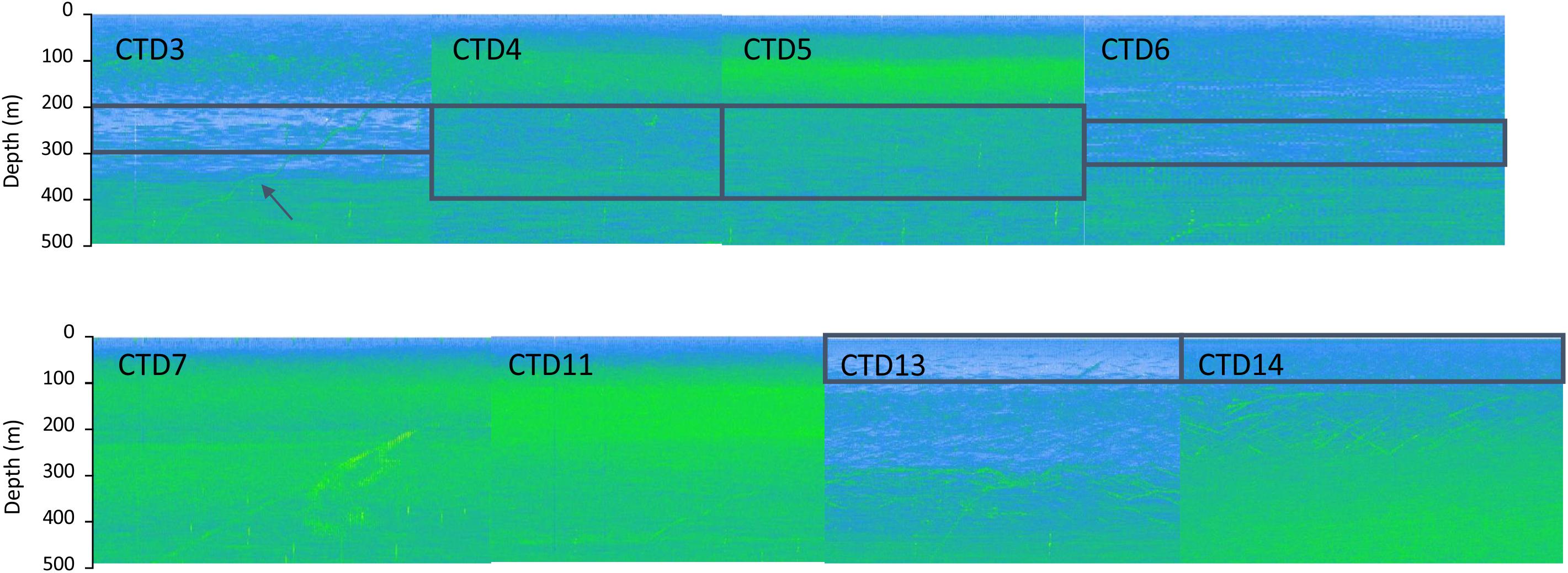
Figure 14. Hydroacoustic data recorded during the upcast of the CTD-hydrocasts (arrow indicates CTD-upcast). Solely the upper 500 m of the hydroacoustic data are shown together with boxes that represent depths of peak methane concentrations. During hydrocasts CTD-7 and CTD-11, methane concentrations did not show a distinct plume and were below 5 nM, thus only slightly elevated compared to methane concentrations in atmospheric equilibrium. Increased methane concentrations were only observed in low backscatter regions.
Methane Anomalies in the Lower Water Column
Methane Fluxes From Two Different Seep Sites
The methane flux at FWCR is lower than the methane flux at SSFR (Table 1). The difference in flux reflects the lower methane concentrations in the water above FWCR when compared to SSFR. Although a much larger area was sampled at FWCR (4.5 km2) in contrast to SSFR (0.01 km2), we focused on carbonate paved seafloor and flare locations in both areas. Seemingly, FWCR was a less active seepage site than SSFR during our investigations. Fluxes above SSFR vary considerably, due to the large temporal variations in methane concentrations. The variable methane concentrations in turn are due to bubble emissions, which have been hydroacoustically observed as flares (Bohrmann and SO266 Shipboard Participants, 2019). Current speed has been rather stable between 21 and 37 mm s–1 at SSFR, thus, affecting the flux estimates less than the methane concentrations.
Our flux estimates are based on several assumptions. First, we assumed stable methane concentrations over time for the period of which methane concentrations were averaged to obtain a flux estimate. For example, we summarized all methane concentrations of water samples collected above SSFR in a grid-like fashion during CTD-12 assuming that the concentrations remained similar over ∼3 h. For data obtained above FWCR, the period is longer as data of three hydrocasts were combined. However, we found methane concentrations of 5 nM to be a common concentration near the seafloor of FWCR. The temporal variability of methane concentrations was considerably higher in water above SSFR, thus, we sampled the grid three times. Second, we estimated methane fluxes from the water below our lowermost water samples. This is due to generating a surface based on the lowermost samples, which is located ∼5 m above the seafloor. Hence, our estimates do not include any methane horizontally spread in the 5 m bottom layer outside of our surface area, i.e., fluxes might be higher than our estimates. Third, as we sampled transects instead of grids and focused sampling water above carbonate patches at FWCR, we might have included areas of seepage more than areas of non-seepage. However, the arbitrarily chosen background station (CTD-7; Figure 5D) showed similar methane concentrations. Finally, the uncertainty of the estimated fluxes is due to the precision of the methane concentration and current measurements. The latter one causes larger uncertainties and thus a range of velocities and directions were used to evaluate the error (Table 1). Considering all assumptions, we regard the flux estimates to be valid within an order of magnitude. However, our flux estimates do not include any methane that remained in bubbles in the investigated water volumes. Therefore, the flux estimates underestimate methane contribution to the SCS offshore Taiwan.
The overall range of methane fluxes fits to reported values. Torres et al. (2002) measured fluxes using a benthic chamber that varied between 1 and 90 mmol m–2 d–1 depending on the dominant chemoautotrophic community. The authors measured higher fluxes above sediments covered with bacterial mats and low fluxes in areas covered with clams. Mau et al. (2006) used the same approach for estimation as this study and derived fluxes of 1.1–15.3 mmol m–2 d–1 above mud extrusions offshore Costa Rica. Bubble emissions were not observed during that study. Therefore, the discrepancy between our flux estimates offshore Taiwan and those reported ones result most likely from bubble emissions.
The estimated methane fluxes from the two seep-areas are approximately two orders of magnitude higher than sea to air fluxes. We estimated fluxes from the sediment into the water column to range between 0.1 and 80 mmol m–2 d–1 whereas different studies reported sea to air fluxes of 0.4–15.6 μmol m–2 d–1 for the SCS (Rehder and Suess, 2001; Mau et al., 2007; Zhou et al., 2009; Brunskill et al., 2011; Ma and Cui, 2013; Ye et al., 2016; Tseng et al., 2017) (Supplementary Table S4). The difference accounts to ∼90 μmol m–2 d–1 considering the lower seep flux of FWCR. Aerobic MOxs in the water column average to be 0.02 nM d–1 with a median of 0.01 nM d–1 (all values). Depth integration of these values (1120 m for SSFR and 1340 m for FWCR) would yield a flux of 11.2–26.8 μmol m–2 d–1. This suggests that aerobic methanotrophs oxidize ∼10% of the emitted methane at seep sites while the remaining 90% are most likely distributed and oxidized farther away from the seepage sites to finally form the background methane concentration of the seas (2 nM). The comparison of our derived seep fluxes with sea-air fluxes indicate the importance of the ocean as a sink.
Variability of Methane Seepage From SSFR and Source Location
We observed a change in ocean current direction that we speculate to explain part of the variability of dissolved methane concentrations. While dissolved methane concentrations ranged up to μM-scale during the first survey, the latter two surveys showed lower concentrations. The variability of methane concentration in the vicinity of bubble streams is well known and reported (e.g., Leifer et al., 2006; Schneider von Deimling et al., 2011). However, during this study the ocean current direction changed. Water moved east during the first survey, but to the north/north-west during the second and third survey (Figure 6). Measurements of the first survey thus suggest a methane plume drifting from the NW of the mound to the south by the currents, which we captured during our first grid sampling. The second and third survey show punctual elevated methane concentrations on the NW-side of the carbonate mound and the plume left the box at this side, thus, we missed sampling the plume. Although our data indicated a relation of ocean current direction and dissolved methane concentrations, a change in methane bubble emission from the ground cannot be excluded.
The partly higher concentrations in the upper layer (∼10 m above ground) we interpret to be due to the release of methane from bubbles. For example, during the third survey, 344 nM methane occurred at ∼5 m above the seafloor, but 963 nM at ∼10 m above ground. Most likely, a bubble was caught while closing a Niskin bottle to sample water. Peak concentrations always appeared on the NW side of SSFR; we assume a punctual source there (Figure 6 and Supplementary Figure S2).
Widespread Methane Anomaly at FWCR
Although methane concentrations were generally much lower in comparison to the ones found above SSFR, methane concentrations above the atmospheric equilibrium concentration appeared to be consistent over a wide area of FWCR. The methane concentration in atmospheric equilibrium would be 3.6 nM according to the temperature and salinity of the water, but we measured a minimum of 3.9 nM in the entire investigated FWCR area. Measured values range up to 18.2 nM with an average of 6.2 nM and a median of 5.7 nM (Figures 5A–C). We expected increased methane concentrations above two carbonate patches, which indicate active seep systems, but instead found elevated values in water above the southern part of the ridge where hydroacoustically detected flares indicated bubble emissions, but no carbonates were observed (Bohrmann and SO266 Shipboard Participants, 2019). Moreover, methane concentrations above SYAER, a ridge to the east, were below equilibrium values even at 3.5 m above the seafloor.
At FWCR elevated methane concentrations in an area of 4.5 km2 point to a continuous seepage. If we consider background methane concentrations above that area and would fill the investigated water volume of 0.1 km3 with the output discussed above (0.016 mol s–1), it would take 5 h to get the calculated methane inventory above FWCR (300 mol). This time ignores any loss by current advection and turbulent diffusion. As it is unlikely that we sampled water while methane rich fluids or bubbles discharged shortly before sampling, we hypothesize continuous seepage at least over the time of our investigation of 13 days. Data of SSFR support our hypothesis. Particularly during the second survey crossing the carbonate mound, 13 out of 24 samples had methane concentrations below the equilibrium concentration (Figures 6C,D). SSFR appeared as an active seep site with gas emission and chemosynthetic communities in a carbonate-paved environment (Bohrmann and SO266 Shipboard Participants, 2019), still, methane concentrations were partly below equilibrium values. Hence, it appears that seepage at FWCR is not as vigorous with strong bubble emissions as in the small area investigated at SSFR (0.01 km2), but that methane rich fluids and gas constantly discharge over a wide area.
Methane Release Caused by Coring
We investigated methane concentrations, aerobic MOx-rates, and the abundance of pmoA transcripts after (1) taking a gravity core (CTD-3) and (2) after MeBo drilled in a gas-rich area and gas was emitted (CTD-8). The purpose was to explore the effect of drilling for the ocean environment. However, water samples after coring showed similar methane concentrations as measured before and in the area of FWCR (Figure 5D). Aerobic MOx-rates were also similar as previously measured in the area. Only the relative activity k’ of the bacterial community showed an increase in bottom water (k’ up to 0.0057 d–1, CTD-8) after the gas emission due to MeBo-drilling. Although the number of transcripts of pmoA did not show a trend of increase after MeBo-drilling, the transcript to gene abundance ratio was higher as comparing data at similar depth. Additionally, the relative abundance of methanotrophic bacteria in the microbial community accounted for up to 14.7% of the total reads at cDNA level, greater than that at DNA level. It is thus likely that short-term methane release caused by drilling are insufficient to generate an observable methane plume, but has an observable effect on the active microbial community. The community composition sampled after MeBo-drilling (CTD-8) was similar to the composition found in other samples of the deep water (Figure 11). Hence, we speculate that the methane emission induced a rapid increase of the activity of methanotrophs in the water column whereas an inoculation of methanotrophs from suspended sediment due to the removal of the coring equipment appears less likely.
Conclusion
Offshore southwest Taiwan, elevated methane concentrations occurred in the uppermost 400 m of the water column and at seepage sites at Four Way Closure Ridge and Southern Summit Formosa Ridge, which were partly associated with authigenic carbonates. The main findings concerning the methane enriched upper water column comprise:
• Elevated methane concentrations appear not uniformly distributed. Peak methane concentrations occur in different depth, which seem linked to water mass interactions in the ocean.
• The zones of elevated methane concentrations in the upper water column correlate with depths of hydroacoustic low backscatter, but not with zooplankton migration or fluorescence as indicator of phytoplankton occurrence. Based on our data, elevated methane concentrations in the upper water column appear in ocean depth with low suspended matter and thus possibly less microbial competition.
• Methane concentrations and aerobic MOxs correlate with water temperatures above 10°C and 20°C, respectively. It seems, that microbes generating and consuming methane do find their optimum temperature in the warmer, upper water column. Our 16S rRNA and pmoA results confirm that temperature was the main driver of community compositions of potential methanotrophs in the water column of the northern SCS.
Concerning elevated methane concentrations at the FWCR and SSFR seep sites in the lower water column (>1000 m water depth), we concluded the following:
• Increased methane concentrations appear to originate from long-term seepage. Short-term gas emissions caused by core drilling did not increase methane concentrations in the ocean, but caused an increase in the activity of methanotrophic microbes, who appeared rapidly to respond to elevated methane concentrations. Apparently, only long-term seepage can generate methane anomalies such as the widespread methane anomaly above FWCR.
• Methane concentrations and flux estimates at a bubble emission site above SSFR appear to vary partly due to ocean current direction as was evaluated by repetitive grid sampling.
• Methane fluxes from both seep regions are similar to flux estimates from other seep sites in the world. These fluxes are two orders of magnitude higher than sea to air fluxes, which indicates the sink capacity of the deep waters of SCS diluting and oxidizing methane.
Data Availability Statement
The datasets analyzed for this study can be obtained from PANGAEA (https://www.pangaea.de/). The following links specify associated data with this article: https://doi.pangaea.de/10.1594/PANGAEA.900980, https://doi.pangaea.de/10.1594/PANGAEA.900661, https://doi.pangaea.de/10.1594/PANGAEA.900952, https://doi.pangaea.de/10.1594/PANGAEA.915954, https://doi.pangaea.de/10.1594/PANGAEA.915990, and https://doi.pangaea.de/10.1594/PANGAEA.916201. The obtained sequences were deposited in GenBank under the Bio-project accession number: PRJNA592351.
Author Contributions
GB and SL acquired funding for, organized and managed the research cruise. SM planned sampling strategy and collected data on board together with T-HT and J-NC. SM measured methane concentration and aerobic microbial methane oxidation rates on board. T-HT and J-NC collected and analyzed molecular biological samples. L-HL and P-LW were involved in sampling design, analysis and sequence interpretation together with T-HT and J-NC and provided financial support. MB and CS post-processed ADCP-data and hydroacoustic data, respectively. SM took the lead in writing the manuscript, but T-HT and J-NC wrote the molecular biological section, MB and CS the method sections of ADCP and hydroacoustic data, respectively. All authors contributed to discuss the collected data. All authors contributed to the article and approved the submitted version.
Funding
This work was part of the Taiwan-German cooperation. The Federal Ministry of Education and Research (BMBF) (03G0266A) funded the SO266 – TaiDrill project “Influence of tectonic processes on hydrate distribution and dynamics at Taiwan’s margin, MeBo drillings during R/V SONNE cruise SO266.” Funding included the position of SM. MB was funded by KMS, the Center for Interdisciplinary Marine Science in Kiel, Germany. The Taiwan Ministry of Science and Technology supported SL TaiGer project (MOST108-2611-M002-003).
Conflict of Interest
The authors declare that the research was conducted in the absence of any commercial or financial relationships that could be construed as a potential conflict of interest.
Acknowledgments
We are indebted to the captain, crew, and the scientific research party of the research vessel SONNE (cruise SO266). We are grateful to Laura Kramer, Gero Wetzel, and Dr. Thomas Pape for their help collecting samples and especially to Janice Malnati for analyzing samples on board. We like to thank Laura Kramer and Paul Wintersteller to record and analyze hydroacoustic data. We are grateful to the principal investigator Prof. Christian Berndt apart from the co-authors GB and SL to get the opportunity to participate on the cruise.
Supplementary Material
The Supplementary Material for this article can be found online at: https://www.frontiersin.org/articles/10.3389/fmars.2020.00543/full#supplementary-material
Footnotes
References
Barnes, R. O., and Goldberg, E. D. (1976). Methane production and consumption in anoxic marine sediments. Geology 4, 297–300.
Blees, J., Niemann, H., Erne, M., Zopfi, J., Schubert, C. J., and Lehmann, M. F. (2015). Spatial variations in surface water methane super-saturation and emission in Lake Lugano, southern Switzerland. Aquat. Sci. 77, 535–545. doi: 10.1007/s00027-015-0401-z
Bogard, M. J., Del Giorgio, P. A., Boutet, L., Chaves, M. C. G., Prairie, Y. T., Merante, A., et al. (2014). Oxic water column methanogenesis as a major component of aquatic CH4 fluxes. Nat. Commun. 5:5350.
Bohrmann, G. and SO266 Shipboard Participants (2019). MeBo200 Methane Hydrate Drillings Southwest of Taiwan First Results from the R/V Sonne Cruise SO266. AGU Fall Meeting. Washington, DC: American Geophysical Union.
Bowin, C., Lu, R.-S., Lee, C.-S., and Schouten, H. (1978). Plate convergence and accretion in Taiwan–Luzon region. Am. Assoc. Petr. Geol. Bull. 62, 1645–1672.
Bragina, A., Berg, C., Müller, H., Moser, D., and Berg, G. (2013). Insights into functional bacterial diversity and its effects on Alpine bog ecosystem functioning. Sci. Rep. 3:1955.
Brooks, J. M., Reid, D. F., and Bernhard, B. B. (1981). Methane in the upper water column of the Northwestern Gulf of Mexico. J. Geophys. Res. 86, 11029–11040.
Brunskill, G. J., Burns, K. A., and Zagorskis, I. (2011). Natural flux of greenhouse methane from the Timor Sea to the atmosphere. J. Geophys. Res. 116:G02024.
Bussmann, I., Matousu, A., Osudar, R., and Mau, S. (2015). Assessment of the radio 3H-CH4 tracer technique to measure aerobic methane oxidation in the water column. Limnol. Oceanogr. Methods 13, 312–327. doi: 10.1002/lom3.10027
Caress, D. W., and Chayes, D. N. (1995). “New software for Processing Sidescan Data from Sidescan-Capable Multibeam Sonars,” in Proceedings pf the IEEE Oceans ’95, (San Diego, CA: IEEE).
Chen, C.-T. A., and Tseng, H.-C. (2006). Abnormally high CH4 concentrations in seawater at mid-depths on the continental slopes of the Northern South China Sea. Terr. Atmos. Ocean Sci. 17, 951–959.
Chi, W.-C., Chen, L., Liu, C.-S., and Brookfield, M. (2014). Development of arc–continent collision mélanges: linking onshore geological and offshore geophysical observations of the Pliocene Lichi Mélange, southern Taiwan and northern Luzon arc, western Pacific. Tectonophysics 636, 70–82. doi: 10.1016/j.tecto.2014.08.009
Chi, W.-C., Reed, D. L., Liu, C.-S., and Lundberg, N. (1998). Distribution of the bottom-simulating reflector in the offshore Taiwan collision zone. Terr. Atmos. Ocean. Sci. 9, 779–794.
Conrad, R. (2009). The global methane cycle: recent advances in understanding the microbial processes involved. Environ. Microbiol. Rep. 1, 285–292. doi: 10.1111/j.1758-2229.2009.00038.x
Cynar, F. J., and Yayanos, A. A. (1993). “The oceanic distribution of methane and its flux to the atmosphere over Southern California waters,” in Biogeochemistry of Global Change: Radiatively Active Trace Gases, ed. R. S. Oremland (New York, NY: Chapman-Hall), 551–573. doi: 10.1007/978-1-4615-2812-8_30
Damm, E., Helmke, E., Thoms, S., Schauer, U., Noethig, E., Bakker, K., et al. (2010). Methane production in aerobic oligotrophic surface water in the central Arctic Ocean. Biogeosciences 7, 1099–1108. doi: 10.5194/bg-7-1099-2010
de Angelis, M. A., and Lee, C. (1994). Methane production during zooplankton grazing on marine phytoplankton. Limnol. Oceanogr. 39, 1298–1308. doi: 10.4319/lo.1994.39.6.1298
Degelmann, D. M., Borken, W., Drake, H. L., and Kolb, S. (2010). Different atmospheric methane-oxidizing communities in European beech and Norway spruce soils. Appl. Environ. Microbiol. 76, 3228–3235. doi: 10.1128/aem.02730-09
Dixon, P. (2003). VEGAN, a package of R functions for community ecology. J. Veg. Sci. 14, 927–930. doi: 10.1111/j.1654-1103.2003.tb02228.x
Edgar, R. C. (2013). UPARSE: highly accurate OTU sequences from microbial amplicon reads. Nat. Methods 10, 996–998. doi: 10.1038/nmeth.2604
Edgar, R. C., Haas, B. J., Clemente, J. C., Quince, C., and Knight, R. (2011). UCHIME improves sensitivity and speed of chimera detection. Bioinformatics 27, 2194–2200. doi: 10.1093/bioinformatics/btr381
Feng, D., and Chen, D. (2015). Authigenic carbonates from an active cold seep of the northern South China Sea: new insights into fluid sources and past seepage activity. Deep Sea Res. Part II 122, 74–83. doi: 10.1016/j.dsr2.2015.02.003
Fish, J. A., Chai, B., Wang, Q., Sun, Y., Brown, T. C., Tiedje, J. M., et al. (2013). FunGene: the functional gene pipeline and repository. Front. Microbiol. 4:291. doi: 10.3389/fmicb.2013.00291
Formolo, M. (2010). “The microbial production of methane and other volatile hydrocarbons,” in Handbook of Hydrocarbon and Lipid Microbiology, ed. K. N. Timmis (New York, NY: Springer), 113–126. doi: 10.1007/978-3-540-77587-4_6
Gan, J., Liu, Z., and Hui, C. R. (2016). A three-layer alternating spinning circulation in the South China Sea. J. Phys. Oceanogr. 46, 2309–2315. doi: 10.1175/jpo-d-16-0044.1
Geprägs, P. (2016). Methane Environment Around Cold Seeps - Examples from Antarctica and the Mediterranean. Ph.D. thesis, University of Bremen, Bremen.
Grossart, H.-P., Frindte, K., Dziallas, C., Eckert, W., and Tang, K. W. (2011). Microbial methane production in oxygenated water column of an oligotrophic lake. Proc. Natl. Acad. Sci. U.S.A. 108, 19657–19661. doi: 10.1073/pnas.1110716108
Han, X., Suess, E., Huang, Y., Wu, N., Bohrmann, G., Su, X., et al. (2008). Jiulong methane reef: microbial mediation of seep carbonates in the South China Sea. Mar. Geol. 249, 243–256. doi: 10.1016/j.margeo.2007.11.012
Han, X., Suess, E., Liebetrau, V., Eisenhauer, A., and Huang, Y. (2014). Past methane release events and environmental conditions at the upper continental slope of the South China Sea: constraints by seep carbonates. Int. J. Earth Sci. 103, 1873–1887. doi: 10.1007/s00531-014-1018-5
Hayes, D. E., and Lewis, S. D. (1984). A geophysical study of the Manila Trench, Luzon, Philippines 1. Crustal structure, gravity, and regional tectonic evolution. J. Geophys. Res. 89, 9171–9195.
Hinrichs, K.-U., and Boetius, A. (2002). “The anaerobic oxidation of methane: New insights in microbial ecology and biogeochemistry,” in Ocean Margin Systems, eds G. Wefer, D. Billett, D. Hebbeln, B. B. Jørgensen, M. Schlüter, and T. C. E. Van Weering (Berlin: Springer Verlag), 457–477. doi: 10.1007/978-3-662-05127-6_28
Hu, J., Pan, J., Guo, X., and Zheng, Q. (2011). Introduction to the special section on regional environmental oceanography in the South China Sea and its adjacent areas (REO-SCS). J. Oceanogr. 67, 359–363. doi: 10.1007/s10872-011-0063-y
Huang, C.-Y., Yuan, P.-B., Lin, C.-W., Wang, T.-K., and Chang, C.-P. (2000). Geodynamic processes of Taiwan arc-continent collision and comparison with analogs in Timor, Papua New Guinea, Urals and Corsica. Tectonophysics 325, 1–21. doi: 10.1016/s0040-1951(00)00128-1
Huang, D., Zhang, X., Jiang, Z., Zhang, J., Arbi, I., Jiang, X., et al. (2017). Seasonal fluctuations of ichthyoplankton assemblage in the northeastern South China Sea influenced by the Kuroshio intrusion. J. Geophys. Res. Oceans 122, 7253–7266. doi: 10.1002/2017jc012906
Isobe, A., and Namba, T. (2001). The circulation in the upper and intermediate layers of the South China Sea. J. Oceanogr. 57, 93–104.
Jakobs, G., Holtermann, P., Berndmeyer, C., Rehder, G., Blumenberg, M., Jost, G., et al. (2014). Seasonal and spatial methane dynamics in the water column of the central Baltic Sea (Gotland Sea). Cont. Shelf Res. 91, 12–25. doi: 10.1016/j.csr.2014.07.005
Jilan, S. (2004). Overview of the South China Sea circulation and its influence on the coastal physical oceanography outside the Pearl River Estuary. Cont. Shelf Res. 24, 1745–1760. doi: 10.1016/j.csr.2004.06.005
Johnson, J. E., Mienert, J., Plaza-Faverola, A., Vadakkepuliyambatta, S., Knies, J., Bünz, S., et al. (2015). Abiotic methane from ultraslow-spreading ridges can charge Arctic gas hydrates. Geology 43, 371–374. doi: 10.1130/g36440.1
Karl, D. M., Beversdorf, L., Bjoerkman, K. M., Church, M. J., Martinez, A., and Delong, E. F. (2008). Aerobic production of methane in the sea. Nat. Geosci. 1, 473–478. doi: 10.1038/ngeo234
Karl, D. M., and Tilbrook, B. D. (1994). Production and transport of methane in oceanic particulate organic matter. Nature 368, 732–734. doi: 10.1038/368732a0
Knittel, K., and Boetius, A. (2009). Anaerobic oxidation of methane: progress with an unknown process. Annu. Rev. Microbiol. 63, 311–334. doi: 10.1146/annurev.micro.61.080706.093130
Kolb, S., Knief, C., Stubner, S., and Conrad, R. (2003). Quantitative detection of methanotrophs in soil by novel pmoA-targeted real-time PCR assays. Appl. Environ. Microbiol. 69, 2423–2429. doi: 10.1128/aem.69.5.2423-2429.2003
Koschel, R. (1980). Untersuchungen zur Phosphataffinitat des Planktons in der euphotischen Zone von Seen. Limnologica 12, 141–145.
Kozich, J. J., Westcott, S. L., Baxter, N. T., Highlander, S. K., and Schloss, P. D. (2013). Development of a dual-index sequencing strategy and curation pipeline for analyzing amplicon sequence data on the MiSeq illumina sequencing platform. Appl. Environ. Microbiol. 79, 5112–5120. doi: 10.1128/aem.01043-13
Kulm, L. D., Suess, E., Moore, J. C., Carson, B., Lewis, B. T., Ritger, S. D., et al. (1986). Oregon subduction zone: venting, fauna, and carbonates. Science 231, 561–566. doi: 10.1126/science.231.4738.561
Leifer, I., Clark, J. F., and Chen, R. F. (2000). Modifications of the local environment by natural marine hydrocarbon seeps. Geophys. Res. Lett. 27, 3711–3714. doi: 10.1029/2000gl011619
Leifer, I., Luyendyk, B. P., Boles, J., and Clark, J. (2006). Natural marine seepage blowout: contribution to atmosheric methane. Glob. Biogeochem. Cycles 20:GB3008. doi: 10.1029/2005GB002668
Li, F., Li, L., Wang, X., and Liu, C. (2002). Water masses in the South China Sea and water exchange between the Pacific and the South China Sea. J. Ocean Univ. Qingdao 1, 19–24. doi: 10.1007/s11802-002-0025-5
Lin, C.-C., Lin, A. T.-S., Liu, C.-S., Chen, G.-Y., Liao, W.-Z., and Schnurle, P. (2009). Geological controls on BSR occurrences in the incipient arc-continent collision zone off southwest Taiwan. Mar. Petrol. Geol. 26, 1118–1131. doi: 10.1016/j.marpetgeo.2008.11.002
Lin, Y.-T., Tu, T.-H., Wei, C.-L., Rumble, D., Lin, L.-H., and Wang, P.-L. (2018). Steep redox gradient and biogeochemical cycling driven by deeply sourced fluids and gases in a terrestrial mud volcano. FEMS Microbiol. Ecol. 94:fiy171.
Lipp, J. S., Morono, Y., Inagaki, F., and Hinrichs, K.-U. (2008). Significant contribution of Archaea to extant biomass in marine subsurface sediments. Nature 454, 991–994. doi: 10.1038/nature07174
Liu, C.-S., Huang, I.-L., and Teng, L. S. (1997). Structural features off southwestern Taiwan. Mar. Geol. 137, 305–319. doi: 10.1016/s0025-3227(96)00093-x
Ma, L., and Cui, Y. (2013). Dissolved methane concentration and sea-to-air transfer flux of dissolved methane in the upper seawater of the central and northern South China Sea. J. Trop. Oceanogr. 32, 91–101.
Madeira, F., Park, Y. M., Lee, J., Buso, N., Gur, T., Madhusoodanan, N., et al. (2019). The EMBL-EBI search and sequence analysis tools APIs in 2019. Nucleic Acids Res. 47, W636–W641.
Mau, S., Blees, J., Helmke, E., Niemann, H., and Damm, E. (2013). Vertical distribution of methane oxidation and methanotrophic response to elevated methane concentrations in stratified waters of the Arctic fjord Storfjorden (Svalbard, Norway). Biogeosciences 10, 6267–6278. doi: 10.5194/bg-10-6267-2013
Mau, S., Heintz, M. B., and Valentine, D. L. (2012). Quantification of CH4 loss and transport in dissolved plumes of the Santa Barbara Channel, California. Cont. Shelf Res. 32, 110–120. doi: 10.1016/j.csr.2011.10.016
Mau, S., Römer, M., Torres, M. E., Bussmann, I., Pape, T., Damm, E., et al. (2017). Widespread methane seepage along the continental margin off Svalbard - from Bjørnøya to Kongsfjorden. Sci. Rep. 7:42997.
Mau, S., Sahling, H., Rehder, G., Suess, E., Linke, P., and Soeding, E. (2006). Estimates of methane output from mud extrusions at the erosive convergent margin off Costa Rica. Mar. Geol. 225, 129–144. doi: 10.1016/j.margeo.2005.09.007
Mau, S., Valentine, D. L., Clark, J. F., Reed, J., Camilli, R., and Washburn, L. (2007). Dissolved methane distributions and air-sea flux in the plume of a massive seep field, coal oil point, California. Geophys. Res. Lett. 34:L22603.
McCollom, T. M. (2016). Abiotic methane formation during experimental serpentinization of olivine. Proc. Natl. Acad. Sci. U.S.A. 113, 13965–13970. doi: 10.1073/pnas.1611843113
McGinnis, D. F., Greinert, J., Artemov, Y., Beaubien, S. E., and Wuest, A. (2006). Fate of rising methane bubbles in stratified waters: how much methane reaches the atmosphere? J. Geophys. Res. 111:C09007.
McMurdie, P. J., and Holmes, S. (2013). Phyloseq: an R package for reproducible interactive analysis and graphics of microbiome census data. PLoS One 8:e61217. doi: 10.1371/journal.pone.0061217
Mohanty, S. R., Bodelier, P. L., and Conrad, R. (2007). Effect of temperature on composition of the methanotrophic community in rice field and forest soil. FEMS Microbiol. Ecol. 62, 24–31. doi: 10.1111/j.1574-6941.2007.00370.x
Murrell, J. C. (2010). “The aerobic methane oxidizing bacteria (methanotrophs),” in Handbook of Hydrocarbon and Lipid Microbiology, ed. K. N. Timmis (Berlin: Springer), 1953–1966. doi: 10.1007/978-3-540-77587-4_143
Paulson, J. N., Stine, O. C., Bravo, H. C., and Pop, M. (2013). Differential abundance analysis for microbial marker-gene surveys. Nat. Methods 10, 1200–1202. doi: 10.1038/nmeth.2658
R Development Core Team (2013). R: A Language and Environment for Statistical computing. Vienna: R Foundation for Statistical Computing.
R Development Core Team (2017). R: A Language and Environment for Statistical Computing. Vienna: R Foundation for Statistical Computing.
Reeburgh, W. S. (2007). Oceanic Methane Biogeochemistry. Chem. Rev. 107, 486–513. doi: 10.1021/cr050362v
Reeburgh, W. S., Ward, B. B., Whalen, S. C., Sandbeck, K. A., Kilpatrick, K. A., and Kerkhof, L. J. (1991). Black Sea methane geochemistry. Deep Sea Res. 38, S1189–S1210.
Rehder, G., and Suess, E. (2001). Methane and pCO2 in the Kuroshio and the South China Sea during maximum summer surface temperatures. Mar. Chem. 75, 89–108. doi: 10.1016/s0304-4203(01)00026-3
Reim, A., Lüke, C., Krause, S., Pratscher, J., and Frenzel, P. (2012). One millimetre makes the difference: high-resolution analysis of methane-oxidizing bacteria and their specific activity at the oxic-anoxic interface in a flooded paddy soil. ISME J. 6, 2128–2139. doi: 10.1038/ismej.2012.57
Repeta, D. J., Ferrón, S., Sosa, O. A., Johnson, C. G., Repeta, L. D., Acker, M., et al. (2016). Marine methane paradox explained by bacterial degradation of dissolved organic matter. Nat. Geosci. 9, 884–887. doi: 10.1038/ngeo2837
Riedel, M., Scherwath, M., Römer, M., Veloso, M., Heesemann, M., and Spence, G. D. (2018). Distributed natural gas venting offshore along the Cascadia margin. Nat. Commun. 9:3264.
Ruff, S. E., Kuhfuss, H., Wegener, G., Lott, C., Ramette, A., Wiedling, J., et al. (2016). Methane seep in shallow-water permeable sediment harbors high diversity of anaerobic methanotrophic communities, Elba, Italy. Front. Microbiol. 7:374. doi: 10.3389/fmicb.2016.00374
Schloss, P. D., Westcott, S. L., Ryabin, T., Hall, J. R., Hartmann, M., Hollister, E. B., et al. (2009). Introducing mothur: open-source, platform-independent, community-supported software for describing and comparing microbial communities. Appl. Environ. Microbiol. 75, 7537–7541. doi: 10.1128/aem.01541-09
Schmale, O., Schneider Von Deimling, J., Gülzow, W., Nausch, G., Waniek, J. J., and Rehder, G. (2010). Distribution of methane in the water column of the Baltic Sea. Geophys. Res. Lett. 37:L12604.
Schmale, O., Wäge, J., Mohrholz, V., Wasmund, N., Gräwe, U., Rehder, G., et al. (2018). The contribution of zooplankton to methane supersaturation in the oxygenated upper waters of the central Baltic Sea. Limnol. Oceanogr. 63, 412–430. doi: 10.1002/lno.10640
Schneider von Deimling, J., Rehder, G., Greinert, J., Mcginnis, D. F., Boetius, A., and Linke, P. (2011). Quantification of seep-related methane gas emissions at Tommeliten, North Sea. Cont. Shelf Res. 31, 876–878.
Sibuet, M., and Olu, K. (1998). Biogeography, biodiversity and fluid dependence of deep-sea cold-seep communities at active and passive margins. Deep Sea Res. Part II 45, 517–567. doi: 10.1016/s0967-0645(97)00074-x
Siljanen, H. M., Saari, A., Bodrossy, L., and Martikainen, P. J. (2012). Seasonal variation in the function and diversity of methanotrophs in the littoral wetland of a boreal eutrophic lake. FEMS Microbiol. Ecol. 80, 548–555. doi: 10.1111/j.1574-6941.2012.01321.x
Skarke, A., Ruppel, C., Kodis, M., Brothers, D., and Lobecker, E. (2014). Widespread methane leakage from the sea floor on the northern US Atlantic margin. Nat. Geosci. 7, 657–661. doi: 10.1038/ngeo2232
Stawiarski, B., Otto, S., Thiel, V., Gräwe, U., Loick-Wilde, N., Wittenborn, A. K., et al. (2019). Controls on zooplankton methane production in the central Baltic Sea. Biogeosciences 16, 1–16.
Stolper, D. A., Lawson, M., Davis, C. L., Ferreira, A. A., Santos Neto, E. V., Ellis, G. S., et al. (2014). Formation temperatures of thermogenic and biogenic methane. Science 344, 1500–1503. doi: 10.1126/science.1254509
Tang, K. W., Glud, R. N., Glud, A., Rysgaard, S., and Nielsen, T. G. (2011). Copepod guts as biogeochemical hotspots in the sea: evidence from microelectrode profiling of Calanus spp. Limnol. Oceanogr. 56, 666–672. doi: 10.4319/lo.2011.56.2.0666
Taylor, B., and Hayes, D. E. (1983). “The origin and history of the South China Basin,” in the Tectonic and Geologic Evolution of Southeast Asian Seas and Islands. Geophysical Monograph 27, ed. D. E. Hayes (Washington, DC: American Geophysical Union), 23–56. doi: 10.1029/gm027p0023
Tissot, B. P., and Welte, D. H. (1984). Petroleum Formation and Occurrence. Heidelberg: Springer Verlag.
Torres, L. M., Mcmanus, J., Hammond, D. E., De Angelis, M. A., Heeschen, K. U., Colbert, S. L., et al. (2002). Fluid and chemical fluxes in and out of sediments hosting methane hydrate deposits on Hydrate Ridge, OR, I: hydrological provinces. Earth Planet. Sci. Lett. 201, 525–540. doi: 10.1016/s0012-821x(02)00733-1
Tseng, H.-C., Chen, C.-T. A., Borges, A. V., Delvalls, T. A., and Chang, Y.-C. (2017). Methane in the South China Sea and the Western Philippine Sea. Cont. Shelf Res. 135, 23–34. doi: 10.1016/j.csr.2017.01.005
Tu, T.-H., Wu, L.-W., Lin, Y.-S., Imachi, H., Lin, L.-H., and Wang, P.-L. (2017). Microbial community composition and functional capacity in a terrestrial ferruginous, sulfate-depleted mud volcano. Front. Microbiol. 8:2137. doi: 10.3389/fmicb.2017.02137
Urmann, K., Lazzaro, A., Gandolfi, I., Schroth, M. H., and Zeyer, J. (2009). Response of methanotrophic activity and community structure to temperature changes in a diffusive CH4/O2 counter gradient in an unsaturated porous medium. FEMS Microbiol. Ecol. 69, 202–212. doi: 10.1111/j.1574-6941.2009.00708.x
Valentine, D. L., Blanton, D. C., Reeburgh, W. S., and Kastner, M. (2001). Water column methane oxidation adjacent to an area of active hydrate dissociation, Eel River Basin. Geochim. Cosmochim. Acta 65, 2633–2640. doi: 10.1016/s0016-7037(01)00625-1
Valentine, D. L., Kessler, J. D., Redmond, M. C., Mendes, S. D., Heintz, M. B., Farwell, C., et al. (2010). Propane respiration jump-starts microbial response to a deep oil spill. Science 330, 208–211. doi: 10.1126/science.1196830
Wang, Q., Quensen, J. F., Fish, J. A., Lee, T., Sun, Y., Tiedje, J. M., et al. (2013). Ecological patterns of nifH genes in four terrestrial climatic zones explored with targeted metagenomics using FrameBot, a new informatics tool. mBio 4:e00592-13.
Whiticar, M. J. (1999). Carbon and hydrogen isotope systematics of bacterial formation and oxidation of methane. Chem. Geol. 161, 291–314. doi: 10.1016/s0009-2541(99)00092-3
Wickham, H. (2016). ggplot2: Elegant Graphics for Data Analysis. New York, NY: Springer-Verlag New York.
Wiesenburg, D. A., and Guinasso, J. N. L. (1979). Equilibrium solubilities of methane, carbon monoxide, and hydrogen in water and sea water. J. Chem. Eng. Data 24, 356–360. doi: 10.1021/je60083a006
Wilhelms, A., Larter, S. R., Head, I., Farrimond, P., Di Primio, R., and Zwach, C. (2001). Biodegradation of oil in uplifted basins prevented by deep-burial sterilization. Nature 411, 1034–1037. doi: 10.1038/35082535
Yang, T. F., Chuang, P.-C., Lin, S., Chen, J.-C., Wang, Y., and Chung, S.-H. (2006). Methane venting in gas hydrate potential area offshore of SW Taiwan: evidence of gas analysis of water column samples. Terr. Atmos. Ocean Sci. 17, 933–950.
Ye, W., Zhang, G., Zhu, Z., Huang, D., Han, Y., Wang, L., et al. (2016). Methane distribution and sea-to-air flux in the East China Sea during the summer of 2013: impact of hypoxia. Deep-Sea Res. Part II 124, 74–83. doi: 10.1016/j.dsr2.2015.01.008
Yu, S.-B., Chen, H.-K., and Kuo, L.-C. (1997). Velocity field GPS stations in Taiwan area. Tectonophysics 274, 41–59. doi: 10.1016/s0040-1951(96)00297-1
Zhou, H., Yin, X., Yang, Q., Wang, H., Wu, Z., and Bao, S. (2009). Distribution, source and flux of methane in the western Pearl River Estuary and northern South China Sea. Mar. Chem. 117, 21–31. doi: 10.1016/j.marchem.2009.07.011
Keywords: methane concentration, methane seeps, methane oxidation rate, methanotrophs, ocean current, water column, South China Sea, ocean methane paradox
Citation: Mau S, Tu T-H, Becker M, dos Santos Ferreira C, Chen J-N, Lin L-H, Wang P-L, Lin S and Bohrmann G (2020) Methane Seeps and Independent Methane Plumes in the South China Sea Offshore Taiwan. Front. Mar. Sci. 7:543. doi: 10.3389/fmars.2020.00543
Received: 02 March 2020; Accepted: 15 June 2020;
Published: 13 July 2020.
Edited by:
Xinping Hu, Texas A&M University Corpus Christi, United StatesReviewed by:
S. Emil Ruff, Marine Biological Laboratory (MBL), United StatesYu Hu, Shanghai Ocean University, China
Copyright © 2020 Mau, Tu, Becker, dos Santos Ferreira, Chen, Lin, Wang, Lin and Bohrmann. This is an open-access article distributed under the terms of the Creative Commons Attribution License (CC BY). The use, distribution or reproduction in other forums is permitted, provided the original author(s) and the copyright owner(s) are credited and that the original publication in this journal is cited, in accordance with accepted academic practice. No use, distribution or reproduction is permitted which does not comply with these terms.
*Correspondence: Susan Mau, smau@marum.de