Prediction of the Structural Yield Strength of Saline Soil in Western Jilin Province, China: A Comparison of the Back-Propagation Neural Network and Support Vector Machine Models

Abstract

With the increase in transportation emissions, road diseases in the saline soil area of Jilin Province have become a problem that requires serious attention. In order to improve the subgrade performance, the structural yield strength (SYS) of remolded soil and its factor sensitivity are investigated in this study. Saline soils in Western Jilin are structural in the sense that the bonding strength of soil skeleton is mainly provided by the solidification bond formed by a physicochemical interaction between particles. Its SYS is influenced by its cementation type, genetic characteristics, original rock structure, and environment. Because of the high clay content in Zhenlai saline soil, the specific surface area of soil particles is large, and the surface adsorption capacity of soil particles is strong. In addition, the main cation is Na⁺. The cementation strength of bound water film between soil particles is thus easily affected by water content and salt content, and compaction is also an important factor affecting the strength of soil. Therefore, in this study, the back-propagation neural network (BPNN) model and a support vector machine (SVM) are used to explore the relationship of saline soil’s SYS with its compactness, water content, and salt content. In total, 120 data points collected by a high-pressure consolidation experiment are applied to building BPNN and SVM model. For eliminate redundant features, Pearson correlation coefficient (r_PCC) is used as an evaluation standard of feature selection. The K-fold cross-validation method was used to avoid over fitting. To compare the performance of the BPNN and SVM models, three statistical parameters were used: the determination coefficient (R²), root mean square error (RMSE), and mean absolute percentage deviation (MAPD). The result shows that the average values of R², RMSE, and MAPD of the BPNN model are superior to the values of the SVM. We conclude that the BPNN model is slightly better than the SVM for predicting the SYS of saline soil. Thus, the BPNN model is used to analyze the factor sensitivity of SYS. The results indicate that the influence degrees of the three parameters are as follows: water content > compactness > salt content. This study can provide a basis for estimating the structural yield pressure of soil from its basic properties, and can provide a new way to obtain parameters for geotechnical engineering, ensuring safety while maintaining symmetry in engineering costs.

1. Introduction

Pre-consolidation pressure is not only important for determining the stress history of soil, but is also crucial for compression and deformation analysis of soil under different historical environments [1]. The traditional definition of pre-consolidation pressure is the maximum vertical effective consolidation pressure that the soil has undergone over time, including self-weight pressure and other loads. Clay soils are widely distributed in China. Our research team studied the engineering geology of the representative clay soils. It was found that the rule of change of pre-consolidation pressure with the depth of Xiashu loess in Wuhan is contrary to that of traditional pre-consolidation pressure. The pre-consolidation pressure of the soil samples were determined by the Casagrande method [2]. However, its basic physical properties, hydraulic properties, and mechanical properties are positively correlated with pre-consolidation pressure. In addition, the pre-consolidation pressure of the 20 cm soil layer is higher than that of the 50 cm and 70 cm soil layers of saline soil in Western Jilin [3]. This is due to the solidification bond formed between particles by physicochemical action in the long process of soil formation, which gives the soil skeleton a type of connection strength called structural strength. This kind of soil with structural strength is called structural soil. The pre-consolidation pressure determined by the Casagrands method can only be applied to unstructured soils. For structural soils, the result obtained by this method is called the structural yield strength (SYS) [3]. Butterfield (1979) proposed a more appropriate method to determine SYS by using double logarithmic coordinates [4]. Later, many scholars confirmed the effectiveness of this method [5,6].

Western Jilin Province is one of the most problematic areas of soil salinization in China, and is also a typical seasonal frozen distribution area [7]. The area’s freeze–thaw cycles and dry–wet cycles make this ecosystem fragile, as salt migrates upward and the area of saline soil increases year by year [8]. The geological characteristics of the saline soil have led to aggravation of road diseases in the area, such as salt heaving, frost heaving, and frost boiling [9]. With the development of construction projects and the increase in heavy transportation tasks, it is urgent to improve the subgrade performance of western Jilin. Therefore, in roadbed design, fully considering the SYS of soil and its variations under the influence of various factors is beneficial for the design of the subgrade projects, ensuring safety, and maintaining symmetry in the cost of engineering.

The SYS is usually obtained in a laboratory by a high pressure consolidation test [10], which is time-consuming and expensive [11]. Specific laboratory equipment and experienced geotechnical engineers are needed to obtain reliable SYS. Therefore, it is of great practical significance to establish a mathematical model to determine SYS of soil on the basis of the existing test results [12]. Soil strength and deformation parameters are affected by cementation type, genetic characteristics, the original rock structure, and the environment. Therefore, it is feasible to mine the relationship of soil strength and deformation parameters with their influencing factors, and to predict soil strength and deformation parameters by influencing factors.

Many empirical formulas have been developed by many researchers to reflect the relationship of various parameters and the strength of soil [13,14]. The main drawback of this method is that it ignores the complex mechanism of soil mechanical properties. Regression analysis needs prior knowledge about the nonlinear relationship between parameters and strength, and requires experts to judge the degree of the nonlinearity. When multiple variables are needed for an empirical formula model, there may be multicollinearity problems caused by the correlation between variables [15]. Artificial intelligence (AI) has advanced and shown excellent performance in solving engineering problems compared with traditional methods [16]. Among AI methods, the back-propagation neural network (BPNN) model and support vector machine (SVM) have significant advantages in learning the complex relationship between multi-dimensional data [14,17]. Because BPNN and SVM simplify operations and have better robustness, they are widely used to explore the complex relationship between soil parameters in geotechnical engineering [18]. In this way the BPNN and SVM models were used to explore the relationship between water content, salt content, compactness, and SYS in this study.

The main objective of this study is to develop a prediction model for SYS in the design stage of roadbed engineering, so remolded soil was used. The remolded soil samples with different water content, compactness, and salt content were used for the high-pressure consolidation test, and 120 data points were obtained. To eliminate redundant features, the Pearson correlation coefficient (r_PCC) is an evaluation standard for feature selection. The K-fold cross-validation method was used to avoid overfitting. The BPNN and SVM were used to determining the relationship of SYS with the water content, salt content, and compactness of saline remolded soil in the west of Jilin Province, and the prediction model for SYS was established. Finally, the influence of water content, salt content and compactness on the SYS was studied.

2. Materials and Methods

2.1. Study Area

The western area of Jilin Province is a typical saline soil region in China. The study area is located in the low-lying Songnen Plain, which belongs to a semi-humid and semi-arid climate and is also a typical seasonal frozen soil area. Because of climate and environmental geological factors, salt accumulates more easily on the surface of this area. As a consequence, vegetation in this area is scarce and the ecological environment is fragile (Figure 1). Temperatures below zero in winter last from November to March every year, resulting in surface freezing and upward salinity migration under the influence of the temperature gradient. Precipitation is concentrated from June to August, and the annual precipitation is low. The average precipitation from 2008 to 2018 in Zhenlai is shown in Figure 2, along with the rainfall data collected from China Meteorological Science Data Center. The average precipitation is distributed symmetrically, with the highest in July. In spring and autumn, evaporation is especially strong, so a large amount of salt accumulates on the soil surface year by year under the action of concentration gradient, which makes Jilin Province a typical saline soil area.

The soil samples were collected from Zhenlai County, Jilin Province, on 8 May, 2016 (45°59′41.62″ N, 123°13′46.88″ E, H 137.0 ± 0 m). The location of the sampling points is shown in Figure 1. Soil samples were taken vertically downward and collected every 10 cm of depth at the sampling points. The physical and chemical properties of each soil layer were determined under the guidance of GB/T 50123 (1999). From the surface to 150 cm, the natural density of the samples was 1.60~2.02 g/cm³, and the natural moisture content was 3.20%~17.40%. Due to strong evaporation, the surface layer had the lowest moisture content at 3.20%. The organic content was 0.168%~0.488%. The grain size composition of the soil samples was obtained by particle size analysis, which showed that the sand content of the samples is 5.66%~15.99%, the silt content is 46.92%~57.81%, and the clay content is 26.21%~45.07%. Thus, the saline soil is mainly composed of silt particles, followed by clay particles and sand particles.

In this study, the total soluble salt content is determined using a constant temperature water bath. The total soluble salt in the saline soil was 0.100%~0.408% from the surface to 150 cm. The salt content of the soil samples at 0~70 cm depth was higher than 0.3%, and reduced below 70 cm. The content of Na⁺ and K⁺ was determined by a flame photometer.

Results show that the primary anion in the saline soil is HCO₃⁻, and the primary cation is Na⁺. The high clay and silt content in the saline soil increases the specific surface area and surface energy, and also makes the adsorption capacity of the soil surface stronger [9]. Combined with the high content of Na⁺, a thick diffusion layer forms on the surface of soil particles, which will weaken the bound water connection between particles until it disappears [19].

The curve of ion components with depth is shown in Figure 3. We found that the 40 cm soil layer is the turning point, providing the maximum point of total soluble salt content, HCO₃⁻ content, and SO₄²⁻ content. Therefore, the 40 cm soil layer was selected as the experimental soil for studying the compression characteristics of saline soil in Zhenlai, and the results from the physical and chemical tests are shown in

Table 1. Physical indexes of 40 cm saline soil.

Property	Grain Size Composition			Water Content ω (%)	Optimum Water Content ω0 (%)	Atterberg Limits
	Sand (%)	Silt (%)	Clay (%)			Liquid Limit (%)	Plastic Limit (%)
Value	8.0	53.5	38.5	14.46	20.5	35	17

and

Table 2. Concentration of major chemicals in saline soil.

Soluble Content (%)	Main Ions Concentration(mmol/kg)						Organic Content (%)
	Na+	K+	Mg2+ + Ca2+	SO42−	HCO3−	Cl−
0.408	9.88	0.19	2.99	8.82	12.54	2.40	0.189

.

2.2. Data Preparation

2.2.1. Specimen Design

The high clay and silt content in the saline soil increases the soil’s specific surface area and surface energy and strengthens the adsorption capacity of the soil surface. The higher the content of Na⁺ in the soil, the thicker the bound water film on the outer surface of the soil particles [20]. When the water content is very low, salt crystallizes and forms a bond between soil particles. With an increase of the water content, the strength and the stability of the soil decreases because the salt dissolves in water, which thickens the bound water film and weakens the connection between soil particles. Because the salt content and water content are the factors that affect the thickness and cementation strength of the bound water film between soil particles, they have a great influence on the structural strength of saline soil. The natural salt content of the 40 cm soil layer in western Jilin Province is 0.408%, and the highest was 1.7%, so the salt content was set to 0.0%, 0.4%, 1.0%, and 2.0%. Combined with the natural water content and the optimal water content, the water content was set to 13%, 14%, 15%, 16%, 17%, 18%, 19%, 20%, 21%, and 23%.

Compactness requirements are different for different projects. Compactness requirements in highway projects are generally greater than 90%, and those of other projects are at least 85%. When compactness exceeds 95%, it is difficult to compact the soil. In terms of economic benefits, too much compaction should be avoided. Therefore, considering with the purpose of this test, the compactness was set at 85%, 90%, and 95%, respectively.

2.2.2. High Pressure Consolidation Test

The soil samples were soaked repeatedly in distilled water and desalinated. According to the water content and salinity setting, a certain quantity of soluble salt was added to distilled water to prepare the solution. The prepared solution was evenly sprayed on the desalinated air-dried soil. After full mixing, it was sealed in a freshness-preserving bag and placed in a humidifying cylinder for 24 h to ensure the solution was fully and evenly distributed. The soil sample was compacted into a cutting ring (D = 61.8 mm; H = 20 mm) by the layer-compaction method. A high-pressure consolidation experiment was carried out and 120 data points were obtained by the double logarithmic coordinate method [4]. The double logarithmic coordinate method is to draw the compression curve of soil samples in ln(1 + e)–lg(P) (where e is the void ratio and P is the vertical load) coordinates (as shown in Figure 4). In the double logarithmic coordinate method, the compression curve of a soil sample can be fitted by two straight lines, and the vertical load, corresponding to the intersection point of the two lines, is the structural yield pressure (SYS). The results are shown in

Table 3. The structural yield strength of the remolded saline soil in Zhenlai.

Number	ω (%)	C (%)	S (%)	SYS (kPa)	Number	ω (%)	C (%)	S (%)	SYS (kPa)	Number	ω (%)	C (%)	S (%)	SYS (kPa)
1	13	85	0.0	320	41	16	90	0.0	331	81	19	95	0.0	335
2	13	85	0.4	383	42	16	90	0.4	427	82	19	95	0.4	363
3	13	85	1.0	464	43	16	90	1.0	412	83	19	95	1.0	285
4	13	85	2.0	464	44	16	90	2.0	325	84	19	95	2.0	285
5	13	90	0.0	403	45	16	95	0.0	394	85	20	85	0.0	245
6	13	90	0.4	391	46	16	95	0.4	479	86	20	85	0.4	316
7	13	90	1.0	497	47	16	95	1.0	469	87	20	85	1.0	279
8	13	90	2.0	509	48	16	95	2.0	393	88	20	85	2.0	254
9	13	95	0.0	457	49	17	85	0.0	191	89	20	90	0.0	367
10	13	95	0.4	400	50	17	85	0.4	209	90	20	90	0.4	407
11	13	95	1.0	521	51	17	85	1.0	292	91	20	90	1.0	299
12	13	95	2.0	598	52	17	85	2.0	260	92	20	90	2.0	279
13	14	85	0.0	462	53	17	90	0.0	237	93	20	95	0.0	422
14	14	85	0.4	447	54	17	90	0.4	288	94	20	95	0.4	457
15	14	85	1.0	483	55	17	90	1.0	343	95	20	95	1.0	335
16	14	85	2.0	475	56	17	90	2.0	272	96	20	95	2.0	343
17	14	90	0.0	631	57	17	95	0.0	260	97	21	85	0.0	209
18	14	90	0.4	457	58	17	95	0.4	355	98	21	85	0.4	251
19	14	90	1.0	545	59	17	95	1.0	443	99	21	85	1.0	248
20	14	90	2.0	578	60	17	95	2.0	306	100	21	85	2.0	152
21	14	95	0.0	813	61	18	85	0.0	208	101	21	90	0.0	292
22	14	95	0.4	468	62	18	85	0.4	240	102	21	90	0.4	316
23	14	95	1.0	558	63	18	85	1.0	275	103	21	90	1.0	266
24	14	95	2.0	627	64	18	85	2.0	232	104	21	90	2.0	266
25	15	85	0.0	327	65	18	90	0.0	249	105	21	95	0.0	351
26	15	85	0.4	408	66	18	90	0.4	316	106	21	95	0.4	389
27	15	85	1.0	404	67	18	90	1.0	318	107	21	95	1.0	299
28	15	85	2.0	306	68	18	90	2.0	249	108	21	95	2.0	299
29	15	90	0.0	363	69	18	95	0.0	286	109	23	85	0.0	226
30	15	90	0.4	448	70	18	95	0.4	347	110	23	85	0.4	229
31	15	90	1.0	464	71	18	95	1.0	346	111	23	85	1.0	201
32	15	90	2.0	376	72	18	95	2.0	261	112	23	85	2.0	139
33	15	95	0.0	537	73	19	85	0.0	197	113	23	90	0.0	266
34	15	95	0.4	473	74	19	85	0.4	219	114	23	90	0.4	272
35	15	95	1.0	497	75	19	85	1.0	248	115	23	90	1.0	226
36	15	95	2.0	433	76	19	85	2.0	226	116	23	90	2.0	254
37	16	85	0.0	313	77	19	90	0.0	269	117	23	95	0.0	343
38	16	85	0.4	355	78	19	90	0.4	331	118	23	95	0.4	355
39	16	85	1.0	385	79	19	90	1.0	272	119	23	95	1.0	285
40	16	85	2.0	298	80	19	90	2.0	237	120	23	95	2.0	285

Note: (1) ω: water content; (2) C: compactness; (3) S: salt content; (4) SYS: structural yield strength.

below.

2.2.3. Feature Selection

Feature selection uses some evaluation criteria to select feature subsets from the original feature space and eliminate redundant features, and uses data preprocessing to improve the efficiency of the model [21]. The Pearson correlation coefficient (r_PCC) is an evaluation standard of feature selection. Its values range from −1 to 1. The closer the value is to −1 or 1, the stronger the correlation between features. The formula of the Pearson correlation coefficient is as follows [22]:

$$r_{PCC}=\frac{{{\displaystyle \sum }}_{i=1}^n\left[\left(x_i-\overline{x}\right)\left(y_i-\overline{y}\right)\right]}{\sqrt{{{\displaystyle \sum }}_{i=1}^n{\left(x_i-\overline{x}\right)}^2}\sqrt{{{\displaystyle \sum }}_{i=1}^n{\left(y_i-\overline{y}\right)}^2}}.$$

(1)

The variable x_i is water content, salt content or compactness, and y_i is the structural yield strength. $\overline{x}$ and $\overline{y}$ are the average values of the corresponding variables, and n is the number of samples. Generally speaking, r_PCC < 0.40 indicates weak correlation among variables, 0.40 ≤ r_PCC < 0.70 indicates moderate correlation, 0.70 ≤ r_PCC < 0.9 indicates strong or high correlation, and extremely strong correlation is indicated when 0.90 ≤ r_PCC ≤ 1.

After calculation, the Pearson correlation coefficients of the water content, compactness, and salt content with the structural yield pressure are 1, 1, and 0.402, respectively. There is an extremely strong correlation between water content, compactness, and structural yield pressure. The relationship between salt content and yield pressure is a moderate correlation. Therefore, in this study, the water content, compactness, and moisture content are retained to establish the model.

2.2.4. K-Fold Cross-Validation

Performance evaluation of machine learning models is very important for model selection. K-fold cross-validation is a method to evaluate the model’s performance through sample reuse, which can effectively reduce the prediction error caused by sampling randomness in the modeling process [23]. Therefore, in this study we used K-fold cross-validation for model evaluation and to avoid over-fitting, thus improving the stability and generalization ability of the models.

The main concept behind K-fold cross-validation is to divide the experimental data into K parts, where K-1 parts are the training dataset, and 1 part is the testing dataset. One part was tested alternately; training and testing were carried out K times to obtain the K group model evaluation parameters [24]. Finally, the average value of the evaluation parameters was used to evaluate the different models, and the model with the best evaluation parameters was selected.

Before the establishment of the two prediction models, in order to avoid over-fitting, 120 groups of experimental datasets were divided through five-fold cross-validation.

In order to reduce the influence caused by differences in the order of magnitude, the variables of the training dataset and testing dataset were normalized.

2.3. Methodology

2.3.1. Back Propagation Neural Network (BPNN)

The neural network method is a simplified mathematical model based on the concept of information transmission between biological neurons. Neural networks have been applied in signal processing, pattern recognition, machine control, expert system, and other fields, and have been frequently applied in the field of prediction. BPNN has the strong ability of non-linear mapping and can correctly solve some non-linear problems. The BPNN algorithm uses the Least Mean Square (LMS) learning algorithm as its basic algorithm. The gradient search algorithm is used in the learning process of the network and error propagation is used to correct the weight and to minimize the mean square deviation of the actual output and the expected output of the network. The structure of the BPNN model of this study is shown in Figure 5. Generally, though the BPNN model can get good results for fitting and classification, there are some problems such as weak interpretability, over fitting, and so on. Because of the advantages of BPNN, such as its simple topology, high error precision, easy programming, and strong practicability, the applications of BPNN are extensive, making it one of the most important algorithms in the field of intelligence. In the field of civil engineering, the BPNN has been applied to structural damage detection [25], soft rock strength prediction [26], ground vibration prediction [27], ground subsidence [28,29], engineering cost prediction [30,31], concrete expansion prediction [32], and soil-well potential prediction [33,34], as well as conductivity prediction and other engineering topics [35].

2.3.2. Support Vector Machine (SVM)

Support vector machine (SVM) is a machine learning method based on statistical learning theory [36], Vapnik-Chervonenkis dimension theory and structural risk minimization principles, thereby giving it good generalization ability for future data [37,38]. SVM was originally used to solve pattern recognition problems. With using the insensitive loss function, SVM is gradually applied to solve non-linear regression problems [39]. The SVM is mainly used in tunnel deformation prediction [40], structural damage detection and diagnosis [41], earthquake disaster prediction [42], and saline–alkali degree classification [43] in the field of civil engineering.

For a training dataset

$$(x_i,y_i), i=1,2,\dots ,l,x_i \in R^n, y_i\in R,$$

(2)

the dataset is fitted using linear functions in the high-dimensional feature space, as shown below:

$$y\left(x\right)=w^T\phi \left(x\right)+b.$$

(3)

The nonlinear mapping function φ (x) maps the dataset from the input space to the high-dimensional feature space so that the nonlinear fitting problem in the input space becomes the linear fitting problem in the high-dimensional feature space.

The regression estimation function obtained is

$$f\left(x\right)={{\displaystyle \sum }}_{i=1}^N\left({\alpha }_i-{\alpha }_i^{*}\right)k\left(x_i,x_j\right)+b,$$

(4)

where k(x_i,x_j) is called the kernel function, which is equal to the inner product of two vectors, x_i and x_j, in their characteristic spaces, φ(x_i) and φ(x_j). The kernel function must satisfy the Mercer theorem. The common kernel functions include the linear function, radial basis function, and multi-layer perception function.

The coefficient α_i in the formula can be obtained by solving the following quadratic programming problems:

$$\max -\frac{1}{2}{{\displaystyle \sum }}_{i=1}^N{{\displaystyle \sum }}_{j=1}^N\left({\alpha }_i-{\alpha }_i^{*}\right)\left({\alpha }_j-{\alpha }_j^{*}\right)k\left(x_i,x_j\right)-\epsilon {{\displaystyle \sum }}_{i=1}^N\left({\alpha }_i+{\alpha }_i^{*}\right)+{{\displaystyle \sum }}_{i=1}^N{y}_i\left({\alpha }_i-{\alpha }_i^{*}\right),$$

(5)

$$s.t. {{\displaystyle \sum }}_{i=1}^N{y}_i\left({\alpha }_i-{\alpha }_i^{*}\right)=0,$$

(6)

$$0\le {\alpha }_i,{\alpha }_i^{*}\le C,i=1,2,\dots ,N,$$

(7)

Only a part of (α_i-α_i*) is non-zero in the formula, and the corresponding data points are support vectors. C is a normal number that determines the balance between empirical risk and regularization [44,45].

For a dataset, only the kernel function and regularization parameter C are needed to construct the SVM. The SVM learning algorithm problem is used to solve the constrained quadratic programming problem, and the solution of the quadratic programming (QP) problem is global optimization.

2.3.3. Model Evaluation

In a previous study, Lei (2018) used the R², RMSE and average relative deviation (MRD) to evaluate the predictive effect of the support vector regression (SVR) and BPNN models for the energy loss of a stepped spillway [46]. Zhang (2017) used the R², RMSE and MAPD to evaluate the predictive effect of the general regression neural network (GRNN) and BPNN models for frost heave behavior [34]. According to the significance of the above statistical parameters, this study compares the performance of BPNN and SVM models by using three parameters: the R², RMSE, and MAPD methods.

The formulas of the three statistical parameters are as follows [34]:

(1)

Coefficient of determination (R²), also named the decision coefficient (R²): In a regression analysis, R² is an index that reflects the approximation between the regression predictions and real data. More specifically, R² indicates the proportion of the variance in the dependent variable that is predicted or explained by the predictor variable, also known as the independent variable. When the range of values is 0–1, the closer the values are to 1, the closer the regression predicted values are to the experimental data:

$$R^2=1-\frac{{{\displaystyle \sum }}_{i=1}^N{\left(P\_SY{S}_i-E\_SY{S}_i\right)}^2}{{{\displaystyle \sum }}_{i=1}^N{\left(P\_SY{S}_i\right)}^2}$$

(8)

where P_SYS_i is the predicted SYS, E_SYSi is measured SYS, and N is the total amount of data.

(2)

Root mean square error (RMSE): the RMSE is used to accurately measure the prediction errors of the different models of a particular dataset. The smaller the RMSE, the higher the matching degree between the predicted value and the experimental value:

$$RMSE=\sqrt{\frac{1}{N}{\displaystyle \sum }_{i=1}^N{\left(P\_SY{S}_i-E\_SY{S}_i\right)}^2}$$

(9)

(3)

Mean absolute percentage deviation (MAPD): Because the explanation of the relative error by MAPD is very intuitive, it is often used for model evaluation. The smaller the MAPD, the better the prediction effect of the model:

$$MAPD=\frac{100\%}{N}{{\displaystyle \sum }}_{i=1}^N|\frac{P\_SY{S}_i-E\_SY{S}_i}{P\_SY{S}_i}|.$$

(10)

3. Results

3.1. Determination of BPNN Parameters

In this study, the BPNN model adopts a three-layer network structure, because the BPNN with a hidden layer can simulate a highly complex nonlinear function when the neuron number in the hidden layer is sufficient [47]. There are three input variables: water content, compaction degree, and salt content. The output variable is the SYS. The “logsig” function is applied to the hidden layer, and the “tansig” function is applied to the output layer. The maximum number of iterations is set to 30,000, and the learning rate is set to 0.8.

In addition, the appropriate number of hidden neurons is crucial for network performance. However, it is a complex problem to determine. A BPNN with insufficient neurons will not learn the problem. However, a BPNN with excessive neurons is not only difficult to train, but is also prone to over fitting [48]. Many scholars simply suggest, “test and find it” [49,50]. According to Heaton’s suggestion, when the number of neurons is close to twice that of the input layer, it is a good starting point to find the appropriate neuron number in the hidden layer, and then increase or decrease neurons according to the network performance [51]. At present, there is no authoritative calculation method for the number of hidden neurons, but the range of the number of hidden neurons can be calculated by the following empirical formula [34]:

$$n=\sqrt{n_{in}+n_{out}}+a_0,$$

(11)

where n_in is the number of neurons in the input layer, n_out is the number of neurons in the output layer, and a₀ is the revised value, ranging from 0 to 10.

According to equation (9), the number of hidden neurons of the BPNN in this study ranges from 2 to 12. The evaluation parameters of the 11 models when the number of neurons varies from 2 to 12 are shown in

Table 4. Statistical parameters of BPNN models when the hidden neurons varied.

K-Fold Cross-Validation	Evaluation Parameters	Number of the Hidden Neurons
		2	3	4	5	6	7	8	9	10	11	12
K-1	R2	0.97	0.97	0.97	0.97	0.97	0.97	0.98	0.98	0.97	0.97	0.97
	RMSE	66	62	67	66	66	60	56	56	70	62	62
	MAPD	0.14	0.12	0.14	0.13	0.13	0.12	0.11	0.11	0.14	0.12	0.12
K-2	R2	0.98	0.98	0.97	0.98	0.98	0.98	0.99	0.99	0.98	0.98	0.98
	RMSE	53	52	56	52	50	48	42	42	51	44	45
	MAPD	0.12	0.12	0.13	0.12	0.11	0.11	0.09	0.09	0.12	0.10	0.10
K-3	R2	0.97	0.98	0.97	0.97	0.97	0.98	0.98	0.98	0.97	0.97	0.97
	RMSE	60	57	62	60	59	56	47	47	66	59	59
	MAPD	0.12	0.11	0.13	0.12	0.12	0.11	0.09	0.09	0.15	0.12	0.12
K-4	R2	0.97	0.97	0.96	0.96	0.97	0.97	0.97	0.97	0.96	0.97	0.98
	RMSE	65	65	68	69	64	62	58	58	72	64	56
	MAPD	0.14	0.14	0.15	0.15	0.13	0.13	0.12	0.12	0.15	0.13	0.11
K-5	R2	0.97	0.97	0.97	0.97	0.97	0.97	0.98	0.98	0.96	0.97	0.98
	RMSE	65	65	66	65	64	59	57	57	69	64	58
	MAPD	0.13	0.13	0.13	0.13	0.13	0.12	0.11	0.11	0.14	0.14	0.11

Note: (1) K-1, K-2, K-3, K-4, and K-5 represent the five datasets divided by five-fold cross-validation method; (2) R²: coefficient of determination; (3) RMSE: root mean square error; (4) MAPD: mean absolute percentage deviation.

. The average values of the three statistical parameters of the BPNN models, which are established by the five datasets of five-fold cross-validation, are shown in Figure 6. When the number of neurons is 8, R² is the closest to 1, and the RMSE and MAPD values are the smallest. Therefore, the optimal number of hidden neurons of the BPNN model is 8.

3.2. SVM Parameter Determination

The quality of the parameter settings will affect the prediction effect of the SVM model. In this study, radial basis function (RBF) is used as the kernel function, and the cross validation-grid search method (Grid Search) is used for finding the optimal parameters C and g. C is the penalty factor of the model, which indicates the tolerance of the model to errors. The higher the C value, the lower the tolerance of the model to errors. The g is a parameter of the kernel function, which implicitly determines the distribution of the original data mapped to high-dimensional feature space. The best parameters for the C, g, and mean square error (MSE) of the five datasets are shown in

Table 5. The best parameters C, g and MSE of five datasets.

Projects	Parameters	K-1	K-2	K-3	K-4	K-5
Rough selection results	C	1.7411	16	256	16	256
	g	5.27803	0.108819	0.0625	0.0625	0.0625
	MSE	0.0137	0.0159	0.0095	0.1258	0.0112
Fine selection results	C	1.4142	16	5.65685	16	0.5
	g	0.5	0.176777	0.0625	0.125	0.353553
	MSE	0.0154	0.0155	0.0114	0.0117	0.0122

Note: (1) C: the penalty factor of the model; (2) g: a parameter of the kernel function; (3) MSE: mean square error.

below.

4. Discussions

4.1. Model Performance Comparison

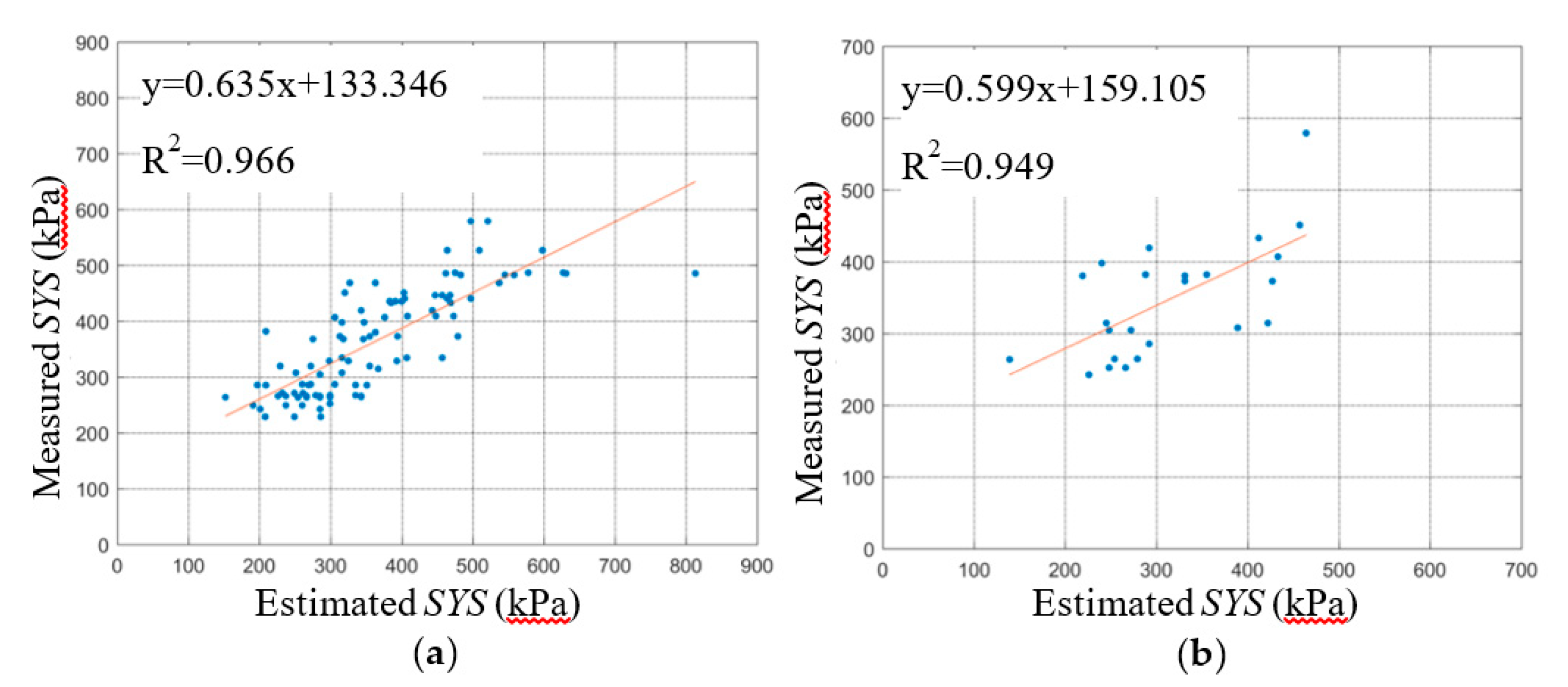
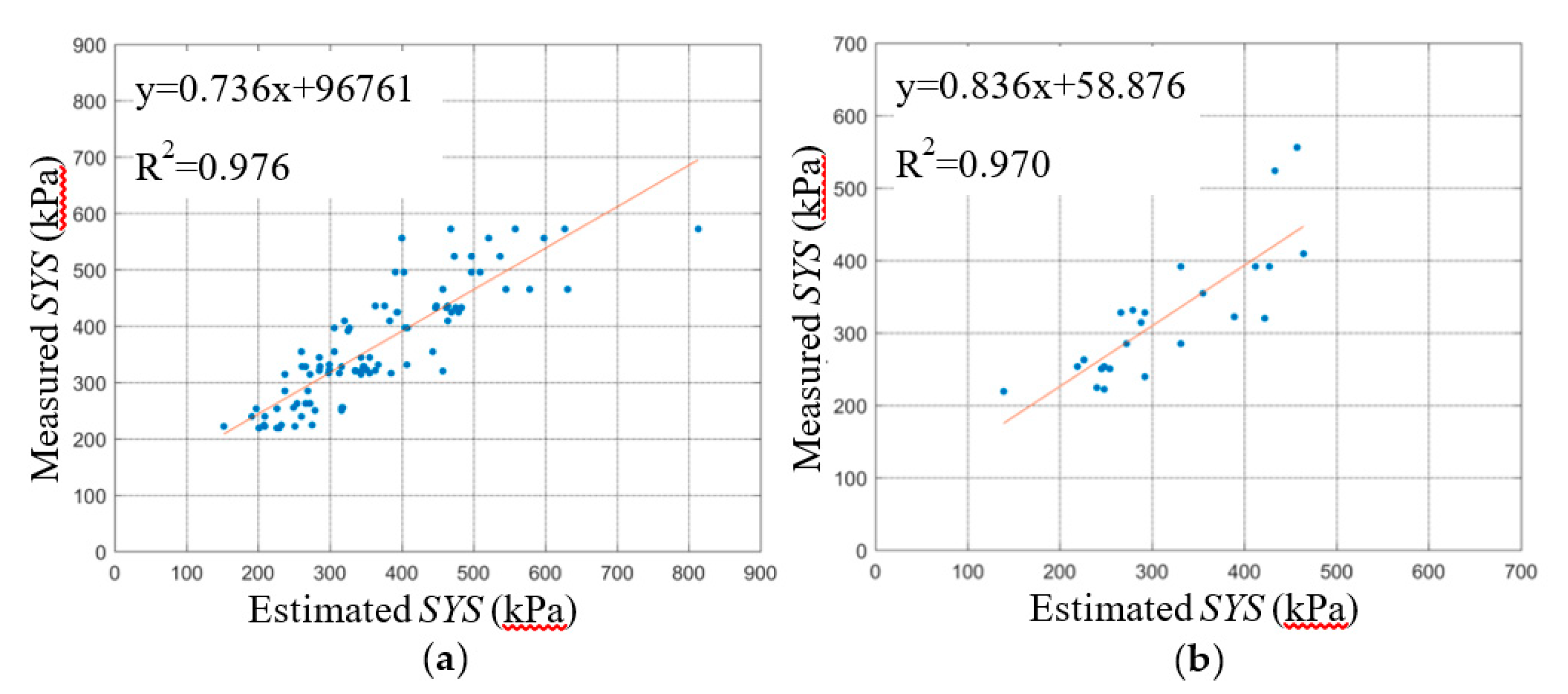
The regression relationships between the predicted SYS and measured SYS of the BPNN and SVM are shown in Figure 7 and Figure 8, respectively, including the training stage and testing stage. A comparison of the BPNN and SVM evaluation parameters in the training stage is shown in

Table 6. The statistical parameters of the BPNN and SVM models (Training stage).

K-Fold Cross-Validation	BPNN			SVM
	R2	RMSE	MAPD	R2	RMSE	MAPD
K-1	0.978	55.523	0.106	0.967	66.791	0.120
K-2	0.986	41.809	0.091	0.976	52.294	0.116
K-3	0.984	47.061	0.087	0.967	65.182	0.131
K-4	0.974	57.946	0.120	0.961	68.578	0.133
K-5	0.976	57.270	0.112	0.967	65.788	0.127
Average	0.980	51.922	0.103	0.967	63.727	0.125

Note: (1) BPNN: back propagation neural network; (2) SVM: support vector model; (3) R²: coefficient of determination; (4) RMSE: root mean square error; (5) MAPD: mean absolute percentage deviation; (5) K-1, K-2, K-3, K-4, and K-5 represent the five datasets divided by five-fold cross-validation method.

, and a comparison of BPNN and SVM evaluation parameters in the testing stage is shown in

Table 7. The statistical parameters and the BPNN and SVM models (Testing stage).

K-Fold Cross-Validation	BPNN			SVM
	R2	RMSE	MAPD	R2	RMSE	MAPD
K-1	0.985	41.554	0.105	0.983	42.370	0.130
K-2	0.943	90.967	0.150	0.931	99.438	0.171
K-3	0.960	69.996	0.168	0.955	72.646	0.177
K-4	0.986	45.334	0.093	0.982	48.486	0.109
K-5	0.982	47.399	0.102	0.966	67.484	0.155
Average	0.971	59.050	0.124	0.963	66.085	0.148

Note: (1) BPNN: back propagation neural network; (2) SVM: support vector model; (3) R²: coefficient of determination; (4) RMSE: root mean square error; (5) MAPD: mean absolute percentage deviation; (5) K-1, K-2, K-3, K-4, and K-5 represent the five dataset divided by five-fold cross-validation method.

.

First, the three statistical indicators of each group of the dataset are analyzed in this section. The R² ranges of the five BPNN models during the training and testing stage were 0.974~0.986 and 0.943~0.986, respectively. The R² ranges of the five SVM models during the training and testing stage were 0.961~0.976 and 0.931~0.983, respectively. The R²_min and R²_max values of the BPNN models during the training and testing stage were greater than those of the SVM models, and the R² ranges of BPNN models were smaller than those of the SVM models. The difference between the R²_max and R²_min of the BPNN and SVM models during the training stage was 0.012 and 0.015 respectively. The difference between the R²_max and R²_min of the BPNN and SVM models during the testing stage was 0.043 and 0.052, respectively. This shows that the R² fluctuation of the BPNN model is smaller than that of the SVM model under different dataset grouping conditions. The explanation degree of independent variable to dependent variable is less affected by dataset grouping.

The RMSE ranges of the five BPNN models during the training and testing stage were 41.809~57.946 and 41.554~90.967, respectively. The RMSE ranges of the five SVM models during training and testing stage were 52.294~68.578 and 42.370~99.438, respectively. The RMSE_max and RMSE_min of the BPNN models during the training and testing stage were less than those of the SVM models. The difference between the RMSE_max and RMSE_min of the BPNN and SVM models during the training stage was 16.137 and 16.284, respectively. The difference between the RMSE_max and RMSE_min of the BPNN and SVM models during the testing stage was 49.413 and 57.068, respectively. The RMSE range of BPNN models is smaller than that of SVM models. The RMSE of the SVM models for the K-2 group of testing dataset was 99.438, which indicates that the prediction error of the SVM models for K-2 group of the testing dataset was greater than other dataset group. Under different dataset grouping conditions, the RMSE fluctuation of the BPNN models was smaller, and the prediction errors of the BPNN models ware less affected by grouping.

The MAPDs of the five BPNN models during the training and testing stage were 0.091~0.120 and 0.102~0.168, respectively. The MAPDs of the five SVM models during the training and testing stage were 0.116~0.133 and 0.109~0.177, respectively. The MAPD_max and MAPD_min of the BPNN models during the training and testing stage were less than or that of SVM models. The MAPDs of the five SVM models during the training stage and the testing stage were all bigger than that of BPNN models. which indicates that the prediction errors of the SVM models were all greater than BPNN models.

The R² and RMSE ranges of the five BPNN models during the training and testing stage were more concentrated than that of the SVM models, which shows that the statistical parameters of the SVM models fluctuate greatly with different dataset groupings. The performance of the SVM models is greatly affected by different dataset groupings. This illustrates that the stability of the BPNN model is better than that of the SVM model.

Next, the average values of the three statistical indicators were analyzed. The average R² of the BPNN models during the training and testing stages was closer to 1 than that of SVM models. The average RMSE of the BPNN during the training and testing stage were 11.805 and 7.035 smaller than that of SVM, respectively. This showed that the prediction error of the BPNN models was smaller than that of SVM models. This indicates that the predicted data for the BPNN models match the experimental data well. The average MAPDs of the BPNN during training and testing stages were 0.022% and 0.024% smaller than that of SVM, respectively. This shows that the relative error of the BPNN model is less than that of the SVM model, so the prediction effects of the BPNN models are better.

The fitting curves between the predicted data of the BPNN and SVM models and the experimental data are shown in Figure 7 and Figure 8. The slope and intercept of the fitting curves also reflect the accuracy of the prediction effect of the model. The closer the slope of the fitting curves is to 1 and the closer the intercept is to 0, the smaller the deviation between the predicted data and the experimental data, and the better the prediction effect of the model. By comparing the fitting lines of the predicted data and the experimental value of the BPNN and SVM model, the predicted effect of the BPNN model is shown to be better overall than that of the SVM. In order to avoid overfitting, the K-fold cross-validation method was used in this study. From the results of the BPNN model parameters, the R² of K-2, K-3, and K-5 datasets in the testing stage are only slightly lower than those in the training stage, and even the R² of K-1 and K-4 datasets in the testing stage are higher than those in the training stage. The results of RMSE and MAPD showed opposite regularity. And the results of the SVM model parameters showed the similar regularity. Moreover, the model parameters of BPNN and SVM models are very stable, neither excellent nor poor. Thus, the performance of BPNN and SVM models is stable, the generalization ability of the model is good for the data of this study, and the generalization ability for external data needs to be explored and improved in future research.

Kogure (1977) [52], Stas (1984) [53], and Degroot (1999) [54] established the empirical models to predict the clay pre-consolidation pressure, and the R² values were all less than 0.80. The model performance was poor and the generalization ability was weak. Karim (2016) proposed a two-fold simple empirical model with R² = 83%, which greatly improved the performance of the model [55]. In this study, the R² results of the pre-consolidation pressure prediction models are all above 90%. Therefore, compared with the existing empirical formula model, the performance of the BPNN and SVM models established in this study are much better.

In the learning process of the BPNN model, the gradient search algorithm is used to correct the weight through error propagation, so that the MSE between the actual output and the expected output is minimized. Because of its strong learning ability, the fitting accuracy of the BPNN model is high. The SVM model is based on the principle of structural risk minimization, which transforms the plane nonlinear problem into a linear problem by mapping data to the high-dimensional feature space. The three independent variables have medium and extremely strong correlation with the dependent variables in this study, and there is no redundancy feature. Therefore, the BPNN and SVM models have good performance and stability. However, the main drawbacks of the BPNN model are that it cannot give a clear mathematical relationship and the results are not interpretable. The performance of the support vector machine mainly depends on the selection of the kernel function, but there is no good method to solve the problem of kernel function selection in different fields.

In addition, in the studies of basic properties, ignoring scale-dependence will make the experimental results deviate from the practical engineering [56]. Considering scale-dependence in the establishment of the model, the prediction results of the model will be closer to the reality and the generalization ability will be better [57,58,59,60]. But the size effect is not taken into account in this study, which may affect the generalization ability of the model. This problem should be fully considered in future research to improve the generalization ability of the model.

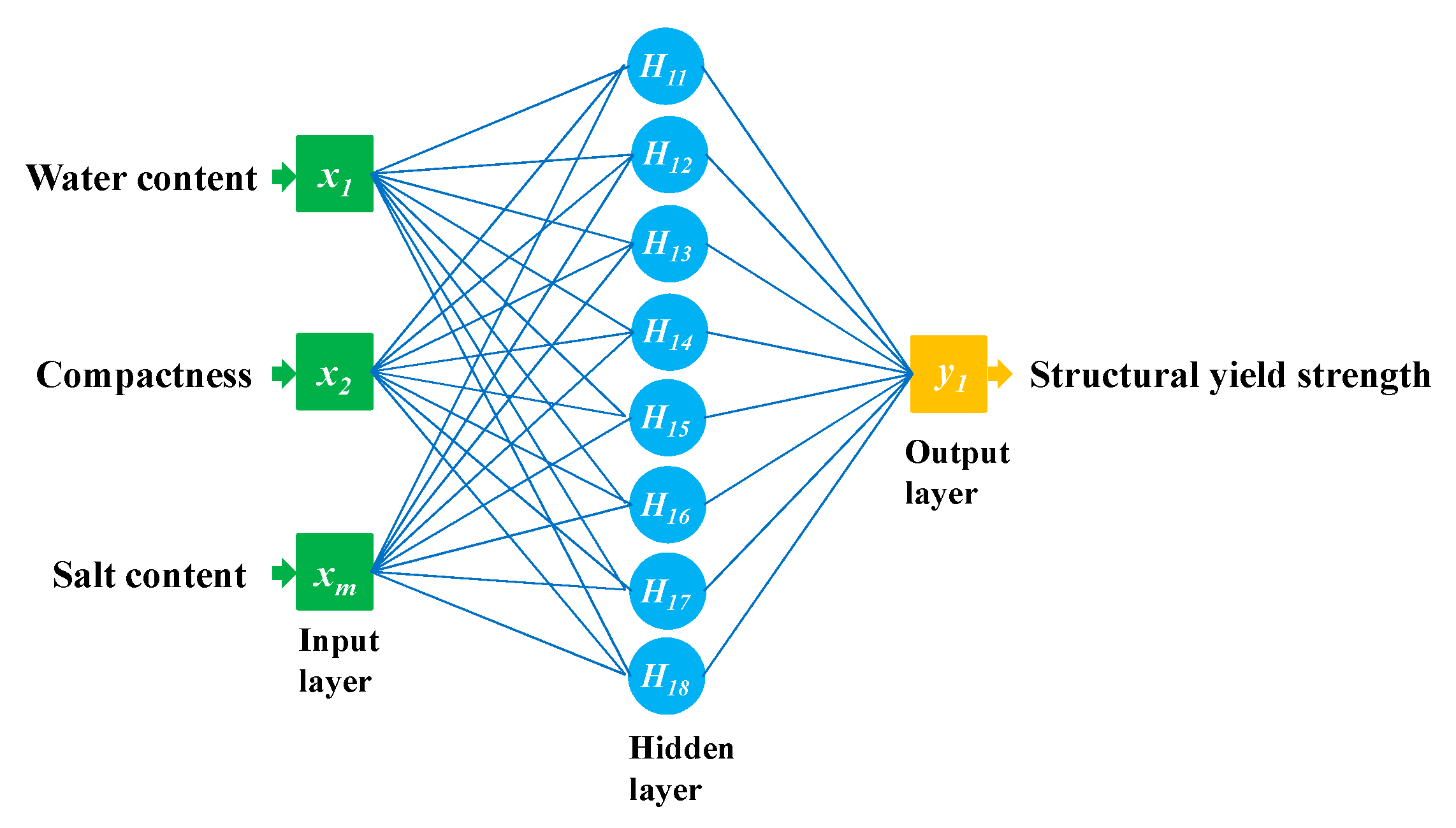
4.2. Sensitivity Analysis

Because the BPNN model is superior to the SVM model, we used it to explore the influence of water content, compactness, and salt content on the SYS. The first model takes compactness and salinity as the input variables, which are recorded as BPNN-1; the second model takes moisture content and salinity as the input variables, which are recorded as BPNN-2; and the third model takes moisture content and compactness as the input variables, which are recorded as BPNN-3. Similarly, according to the K-fold cross-validation method, the datasets are divided into five groups of training datasets and test datasets, and the BPNN models are established and simulated. The statistical evaluation parameters of the three models are shown in

Table 8. Statistical parameters of BPNN models for sensitivity analysis.

Evaluation Parameters	Training Stage			Testing Stage
	R2	RMSE	MAPD	R2	RMSE	MAPD
BPNN-1	0.919	101.005	0.236	0.892	114.365	0.271
BPNN-2	0.966	66.420	0.140	0.949	81.488	0.174
BPNN-3	0.976	56.128	0.118	0.970	62.900	0.142

Note: (1) R²: coefficient of determination; (2) RMSE: root mean square error; (3) MAPD: mean absolute percentage deviation; (4) BPNN-1: dewatering; (5) BPNN-2: de-compaction degree; (6) BPNN-3: desalination content.

.

As shown in Table 8, the average R² of the BPNN-3 during the training and testing stages were greater than 0.969 and were closer to 1 than the average R² of the other two models. This shows that the proportion of variance in the dependent variable that is explained by the independent variable is high in BPNN-3. The R² of BPNN-1 was the smallest, and the average R² value during the training and testing stages was about 0.9. This shows that the proportion of variance in the dependent variable which is explained by the independent variable decreases obviously when the water content of the input variable is removed.

The RMSE average value of BPNN-3 during the training and testing stages was the smallest, which indicates that the error of BPNN-3 was the smallest, so the BPNN-3 matching degree of experimental data and prediction data is the highest. The average RMSE of BPNN-2 during the training and testing stages was 1.186 and 1.296 times that of BPNN-3, respectively. The RMSE average value of BPNN-1 was the largest. The RMSE average value during the training and testing stage was 1.800 and 1.818 times higher than that of BPNN-3, respectively.

The average MAPD of BPNN-3 during the training and testing stages was the smallest, which indicates that the relative error of BPNN-3 was the smallest. The average MAPD of BPNN-2 during the training and testing stages is 1.187 and 1.228 times higher than that of BPNN-3, respectively. The average MAPD of the BPNN-1 model was the largest, and the average MAPD during the training and testing stage was 1.991 and 1.915 times higher than that that of BPNN-3, respectively.

The average values of the three statistical parameters of the BPNN-3 model are the best. The statistical parameters of the BPNN-2 model are better than those of BPNN-1. Because the R² average value of the BPNN-1 model is the smallest when removing the water content of the input variable, and the RMSE and MAPD average values are also larger than BPNN-2 and BPNN-3, the proportion of variance in the dependent variable that is predicted or explained by the independent variable of the model is reduced significantly, and the prediction error and relative error increase significantly when removing the water content of the input variable. Therefore, it can be concluded that the influence degree of each variable is as follows: water content > compaction degree > salt content.

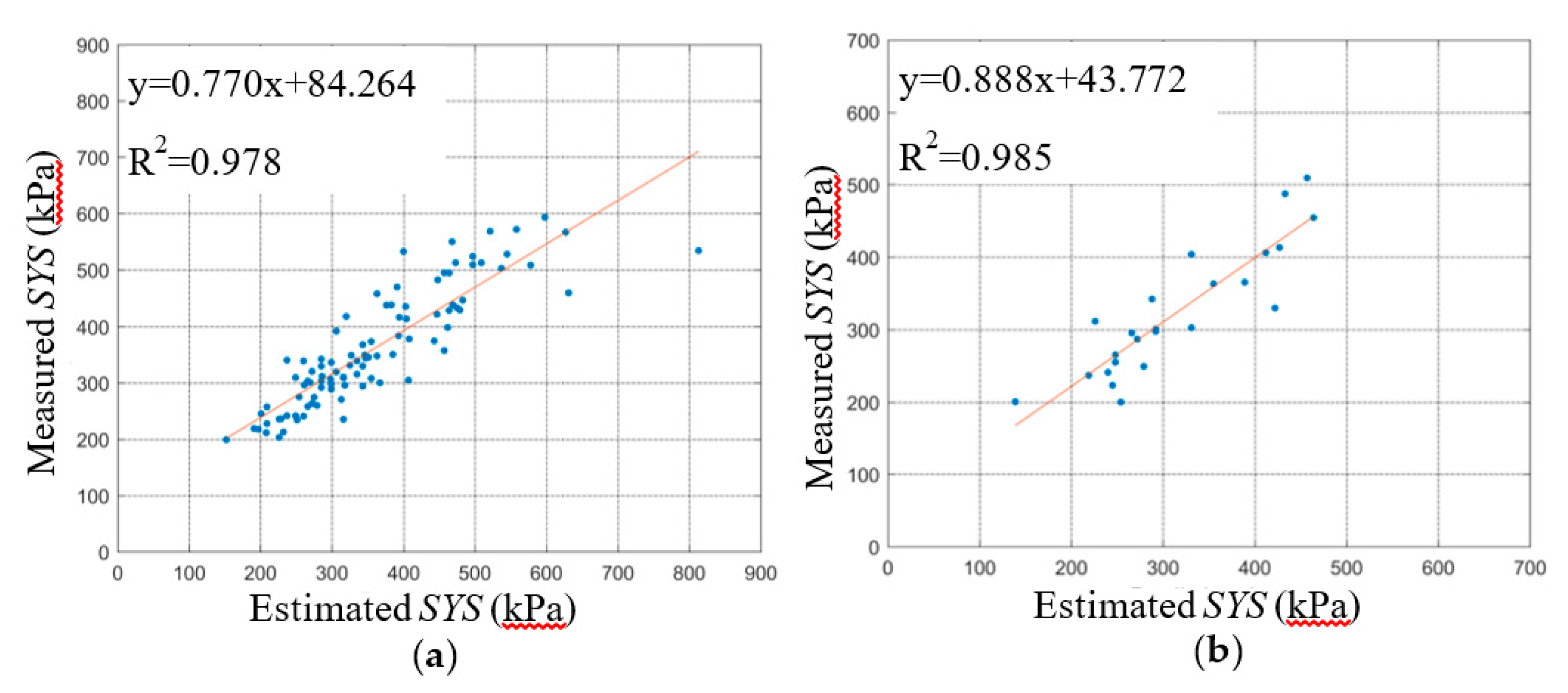
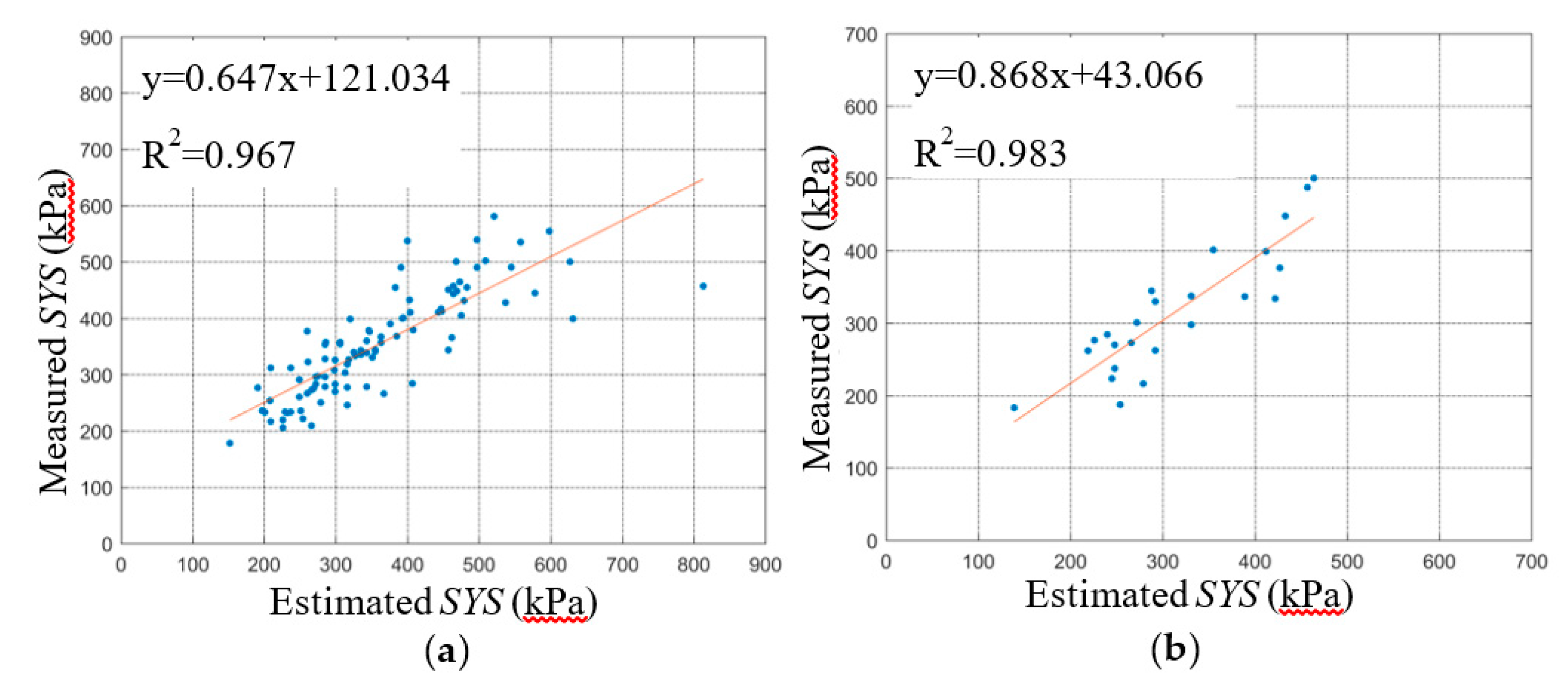
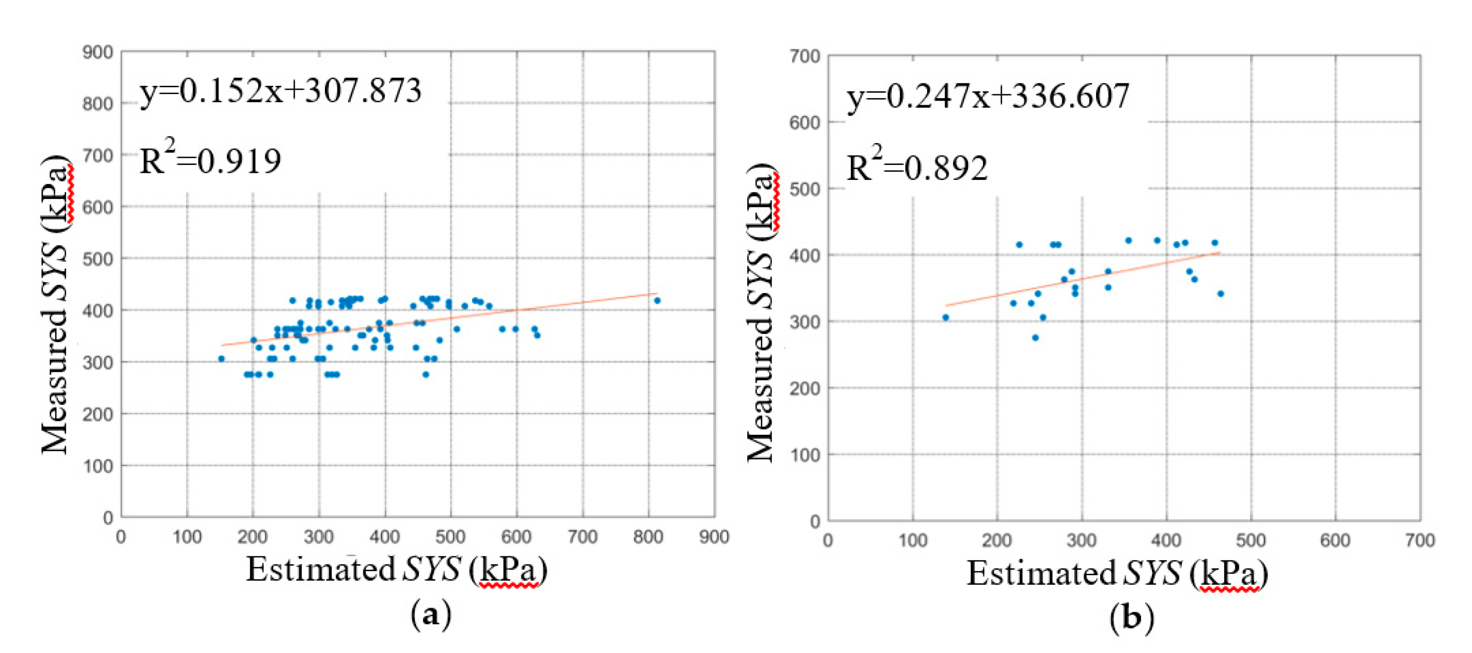
The relationship curve between the estimated SYS and the measured SYS of the BPNN model is shown in Figure 9, Figure 10 and Figure 11. The slope and intercept of the fitting curve also reflect the prediction effect of the model. By comparing the fitting lines between the predicted data of the BPNN-1, BPNN-2, and BPNN-3 models and the experimental data, we found that the predicted results of the BPNN-1 model are the worst, while those of the BPNN-3 model are the best.

5. Conclusions

Structural yield strength (SYS) is a key geotechnical parameter. However, it is impractical for most geotechnical engineering to determine the SYS of the soil layer in a region because of its relatively high technical and cost requirements and because it is time-consuming. Therefore, it is of great engineering significance and economic benefit to establish a prediction model for SYS based on the basic properties of soil.

In this study, the BPNN and SVM models were used to predict the SYS of saline soil in western Jilin Province. Comparing the performance of the BPNN and SVM models, we found that the BPNN model is slightly better than the SVM model. That is, in the BPNN model, the independent variables have a higher explainable degree of dependent variables, the matching degree between the predicted values and experimental values is higher, and the relative error is smaller.

A sensitivity analysis was also carried out by the BPNN model. Based on the same datasets, a set of input variables was removed by an exhaustive method, and two sets of input variables were left to establish the BPNN model; these sets were BPNN-1 (dewatering), BPNN-2 (de-compaction degree), and BPNN-3 (desalination content). The evaluation parameters of the BPNN-3 model are better than those of the BPNN-1 and BPNN-2 models. The evaluation parameters of BPNN-2 are better than BPNN-1. The results show that water content has the greatest influence on the SYS, whereas salt content has the least influence on the SYS. The sensitivity analysis showed that the influence degree of each variable is as follows: water content > compaction degree > salt content.

Comparing the performance of the model established in this study with the traditional empirical formula model based on the internal data set, it was found that the performance of BPNN and SVM models is better. Although K-fold cross-validation is used to avoid the overfitting problem and to improve the generalization ability of the model, the performance of the models based on external datasets needs further research, which is a deficiency of this study.

References

1. Qi, J.; Hu, W.; Ma, W. Experimental study of a pseudo-preconsolidation pressure in frozen soils. Cold Reg. Sci. Technol. 2010, 60, 230–233. [Google Scholar] [CrossRef]
2. Wang, Q.; Chen, J.; Jiang, Z. The New Konwlege on Theory of Preconsolidation Pressure. J. Changchun Univ. Earth Sci. 1996, 26, 59–63. [Google Scholar]
3. Wang, Q.; Kong, Y.; Zhang, X.; Ruan, Y.; Chen, Y. Mechanical Effect of Pre-consolidation Pressure of Structural Behavior Soil. J. Southwest Jiaotong Univ. 2016, 51, 987–994. [Google Scholar] [CrossRef]
4. Yang, A.-W.; Kong, L.-W.; Lu, L.Q. Study on the Shear Structural Yield of Soft Soil Affected by Drainage Condition. Appl. Mech. Mater. 2012, 256–259, 416–421. [Google Scholar] [CrossRef]
5. Butterfield, R. A Natural Compression Law for Soils. Géotechnique 1979, 29, 469–480. [Google Scholar] [CrossRef]
6. Jose, B.T.; Sridharan, A.; Abraham, B.M. Improved technique for estimation of preconsolidation pressure. Géotechnique 1991, 41, 263–268. [Google Scholar] [CrossRef]
7. Hong, Z.-S.; Onitsuka, K. A Method of Correcting Yield Stress and Compression Index of Ariaka Clays for Sample Disturbance. Jpn. Geotech. Soc. 1998, 38, 211–222. [Google Scholar] [CrossRef] [Green Version]
8. Bao, S.C.; Wang, Q.; Bao, X.H. Study on dispersive influencing factors of dispersive soil in western Jilin based on grey correlation degree method. Adv. Energy Sci. Technol. 2013, 291–294, 1096–1100. [Google Scholar] [CrossRef]
9. Zhang, J. Research on the Dispersion Mechanism of the Dispersive Seasonal Frozen Soil in the Western of Jilin Province. Ph. D. Thesis, Jilin University, Changchun, China, 2010. [Google Scholar]
10. Bao, S.; Wang, Q.; Bao, X.; Li, M.; Wang, Z. Biological treatment of saline-alkali soil by Sulfur-oxidizing bacteria. Bioengineered 2016, 7, 372–375. [Google Scholar] [CrossRef] [Green Version]
11. Polidori, E. On the intrinsic compressibility of common clayey soils. Eur. J. Environ. Civ. Eng. 2014, 19, 27–47. [Google Scholar] [CrossRef]
12. Terzaghi, K.; Peck, R.; Mesri, G. Soil Mechanics in Engineering Practice; John Wiley & Sons: Hoboken, NJ, USA, 1996. [Google Scholar]
13. Puri, N.; Prasad, H.; Jain, A. Prediction of Geotechnical Parameters Using Machine Learning Techniques. Procedia Comput. Sci. 2018, 125, 509–517. [Google Scholar] [CrossRef]
14. Drnevich, V.P.; Nagaraj, T.; Murthy, B.R. Prediction of the Preconsolidation Pressure and Recompression Index of Soils. Geotech. Test. J. 1985, 8. [Google Scholar] [CrossRef]
15. Oliveira, P.; Correia, A.; Lemos, L. Numerical prediction of the creep behaviour of an unstabilised and a chemically stabilised soft soil. Comput. Geotech. 2017, 87, 20–31. [Google Scholar] [CrossRef]
16. Tien Bui, D.; Nhu, V.-H.; Hoang, N.-D. Prediction of Soil Compression Coefficient for Urban Housing Project Using Novel Integration Machine Learning Approach of Swarm Intelligence and Multi-Layer Perceptron Neural Network. Adv. Eng. Inform. 2018, 38, 593–604. [Google Scholar] [CrossRef]
17. Khosravani, M.R.; Nasiri, S.; Anders, D.; Weinberg, K. Prediction of dynamic properties of ultra-high performance concrete by an artificial intelligence approach. Adv. Eng. Softw. 2019, 127, 51–58. [Google Scholar] [CrossRef]
18. Das, S.; Samui, P.; Khan, S.Z.; Sivakugan, N. Machine learning techniques applied to prediction of residual strength of clay. Cent. Eur. J. Geosci. 2011, 3, 449–461. [Google Scholar] [CrossRef]
19. Kuo, Y.L.; Jaksa, M.; Lyamin, A.; Kaggwa, W.S. ANN-based model for predicting the bearing capacity of strip footing on multi-layered cohesive soil. Comput. Geotech. 2008, 36, 503–516. [Google Scholar] [CrossRef]
20. Zhang, X.; Liu, S.; Wang, Q.; Wang, G.; Liu, Y.; Peng, W.; Xu, X.; Liu, Y. Experimental Investigation of Water Migration Characteristics for Saline Soil. Pol. J. Environ. Stud. 2019, 28, 1495–1505. [Google Scholar] [CrossRef] [Green Version]
21. Zhang, G.; Germaine, J.T.; Whittle, A.J.; Ladd, C.C. Index properties of a highly weathered old alluvium. Géotechnique 2004, 54, 441–451. [Google Scholar] [CrossRef]
22. Saidi, R.; Bouaguel, W.; Nadia, E. Hybrid Feature Selection Method Based on the Genetic Algorithm and Pearson Correlation Coefficient. In Studies in Computational Intelligence; Springer: Cham, Switzerland, 2019; pp. 3–24. [Google Scholar] [CrossRef]
23. Fu, T.; Tang, X.; Cai, Z.; Zuo, Y.; Tang, Y.; Zhao, X. Correlation research of phase angle variation and coating performance by means of Pearson’s correlation coefficient. Prog. Org. Coat. 2020, 139, 105459. [Google Scholar] [CrossRef]
24. Purushotham, S.; Tripathy, B.K. Evaluation of Classifier Models Using Stratified Tenfold Cross Validation Techniques. In Communications in Computer and Information Science; Springer: Berlin/Heidelberg, Germany, 2011; Volume 270, pp. 680–690. [Google Scholar] [CrossRef]
25. Kohavi, R. A Study of Cross-Validation and Bootstrap for Accuracy Estimation and Model Selection. In Proceedings of the 14th international joint conference on Artificial intelligence, Adelaide, Australia, 10–14 December 2001; Volume 14. [Google Scholar]
26. Wu, X.; Ghaboussi, J.; Garrett, J.H. Use of neural network in detection of structural damage. Comput. Struct. 1992, 42, 649–659. [Google Scholar] [CrossRef]
27. Tonnizam, E.; Armaghani, D.J.; Momeni, E.; Abad, S.V.A.N.K. Prediction of the unconfined compressive strength of soft rocks: A PSO-based ANN approach. Bull. Eng. Geol. Environ. 2014, 74, 745–757. [Google Scholar] [CrossRef]
28. Hajihassani, M.; Armaghani, D.J.; Marto, A.; Tonnizam, E. Ground vibration prediction in quarry blasting through an artificial neural network optimized by imperialist competitive algorithm. Bull. Eng. Geol. Environ. 2014, 74, 873–886. [Google Scholar] [CrossRef]
29. Kim, C.Y.; Bae, G.J.; Hong, S.W.; Park, C.H.; Moon, H.K.; Shin, H.S. Neural network based prediction of ground surface settlements due to tunnelling. Comput. Geotech. 2001, 28, 517–547. [Google Scholar] [CrossRef]
30. Suwansawat, S.; Einstein, H.H. Artificial neural networks for predicting the maximum surface settlement caused by EPB shield tunneling. Tunn. Undergr. Space Technol. 2006, 21, 133–150. [Google Scholar] [CrossRef]
31. Tam, C.M.; Fang, C.F. Comparative cost analysis of using high-performance concrete in tall building construction by artificial neural networks. ACI Struct. J. 1999, 96, 927–936. [Google Scholar]
32. Sarma, K.C.; Adeli, H. Life-cycle cost optimization of steel structures. Int. J. Numer. Methods Eng. 2002, 55, 1451–1462. [Google Scholar] [CrossRef]
33. Wang, B.; Man, T.; Jin, H. Prediction of expansion behavior of self-stressing concrete by artificial neural networks and fuzzy inference systems. Constr. Build. Mater. 2015, 84, 184–191. [Google Scholar] [CrossRef]
34. Penumadu, D.; Zhao, R. Triaxial compression behavior of sand and gravel using artificial neural networks (ANN). Comput. Geotech. 1999, 24, 207–230. [Google Scholar] [CrossRef]
35. Zhang, X.; Wang, Q.; Huo, Z.; Yu, T.; Wang, G.; Liu, T.; Wang, W. Prediction of Frost-Heaving Behavior of Saline Soil in Western Jilin Province, China, by Neural Network Methods. Math. Probl. Eng. 2017, 2017, 1–10. [Google Scholar] [CrossRef] [Green Version]
36. Bayat, H.; Ebrahimi, E.; Ersahin, S.; Hepper, E.; Singh, D.N.; Amer, A.-M.M.M.; Yukselen-Aksoy, Y. Analyzing the effect of various soil properties on the estimation of soil specific surface area by different methods. Appl. Clay Sci. 2015, 116–117, 129–140. [Google Scholar] [CrossRef]
37. Vapnik, V.N. Statistical Learning Theory; Wiley Interscience: Hoboken, NJ, USA, 1998. [Google Scholar]
38. Cristianini, N.; Shawe-Taylor, J. An Introduction of Support Vector Machines and Other Kernel-Based Learning Methods; Cambridge University Press: Cambridge, UK, 2000. [Google Scholar] [CrossRef]
39. Burges, C.J.C. A tutorial on support vector machines for pattern recognition. Data Min. Knowl. Discov. 1998, 2, 121–167. [Google Scholar] [CrossRef]
40. Mukherjee, S.; Osuna, E.; Girosi, F. Nonlinear prediction of chaotic time Series using support vector machines. In Neural Networks for Signal Processing [1997] VII, Proceedings of the 1997 IEEE Workshop 1997, Amelia Island, FL, USA, 24–26 September 1997; IEEE: New York, NY, USA. [Google Scholar] [CrossRef]
41. Ocak, I.; Seker, S.E. Calculation of surface settlements caused by EPBM tunneling using artificial neural network, SVM, and Gaussian processes. Environ. Earth Sci. 2013, 70, 1263–1276. [Google Scholar] [CrossRef]
42. Huo, L.-S.; Li, X.; Yang, Y.-B.; Li, H.-N. Damage Detection of Structures for Ambient Loading Based on Cross Correlation Function Amplitude and SVM. Shock Vib. 2016, 2016, 1–12. [Google Scholar] [CrossRef] [Green Version]
43. Huang, X.; Zhou, Z.; Wang, S. The prediction model of earthquake casuailty based on robust wavelet v-SVM. Nat. Hazards 2015, 77, 717–732. [Google Scholar] [CrossRef]
44. Nurmemet, I.; Sagan, V.; Ding, J.-L.; Halik, Ü.; Abliz, A.; Yakup, Z. A WFS-SVM Model for Soil Salinity Mapping in Keriya Oasis, Northwestern China Using Polarimetric Decomposition and Fully PolSAR Data. Remote Sens. 2018, 10, 598. [Google Scholar] [CrossRef] [Green Version]
45. Vapnik, V. The Nature of Statistical Learning Theory; Springer science & business media: Berlin, Germany, 1995; Volume 6. [Google Scholar]
46. Vn, V. Statistical Learning Theory; Wiley: Hoboken, NJ, USA, 1998; Volume 16. [Google Scholar]
47. Lei, J.; Mingjun, D.; Hongcheng, X.; Haomiao, S. Energy Dissipation Prediction for Stepped Spillway Based on Genetic Algorithm–Support Vector Regression. J. Irrig. Drain. Eng. 2018, 144, 04018033. [Google Scholar] [CrossRef]
48. Kao, L.-J.; Chiu, C.-C.; Lu, C.-J.; Chang, C.-H. A hybrid approach by integrating wavelet-based feature extraction with MARS and SVR for stock index forecasting. Decis. Support Syst. 2013, 54, 1228–1244. [Google Scholar] [CrossRef]
49. Khalaj, G.; Nazari, A.; Pouraliakbar, H. Prediction martensite fraction of microalloyed steel by artificial neural networks. Neural Netw. World 2013, 23, 117. [Google Scholar] [CrossRef] [Green Version]
50. Hegazy, T.; Fazio, P.; Moselhi, O. Developing Practical Neural Network Applications Using Back—Propagation. Comput.-Aided Civ. Infrastruct. Eng. 2008, 9, 145–159. [Google Scholar] [CrossRef]
51. Bishop, C.; Ligne, S. Pattern Recognition and Machine Learning; Springer: Berlin/Heidelberg, Germany, 2006; Volume 1. [Google Scholar]
52. Heaton, J. Introduction to Neural Networks for C#, 2nd ed.; Heaton Research Inc.: St. Louis, MO, USA, 2008. [Google Scholar]
53. Heaton, J. Artificial Intelligence for Humans, Volume 3: Deep Learning and Neural Networks; Heaton Research Inc: St. Louis, MO, USA, 2015. [Google Scholar]
54. Heaton, J. Programming Neural Networks with Encog3 in C#, 2nd ed.; Heaton Research Inc.: St. Louis, MO, USA, 2011. [Google Scholar] [CrossRef]
55. Keiji, K.; Yoshinori, O. Statistical forecasting of compressibility of peaty ground. Can. Geotech. J. 1977, 14, 562–570. [Google Scholar]
56. Stas, C.; Kulhawy, F. Critical Evaluation of Design Methods for Foundations under Axial Uplift and Compression Loading; Final report; Cornell University: Ithaca, NY, USA, 1984. [Google Scholar]
57. DeGroot, D.J.; Knudsen, S.; Lunne, T. Correlations among pc, su and the index properties for offshore clays. In Proceedings of the International Conference on Offshore and Nearshore Geotechnical Engineering, Panvel, India, 2–3 December 1999; pp. 173–178. [Google Scholar]
58. Kootahi, K.; Mayne, P. Index Test Method for Estimating the Effective Preconsolidation Stress in Clay Deposits. J. Geotech. Geoenviron. Eng. 2016, 142, 04016049. [Google Scholar] [CrossRef]
59. Zobeck, T.M.; Fausey, N.R.; Al-Hamdan, N.S. Effect of Sample Cross-Sectional Area on Saturated Hydraulic Conductivity in Tow Structured Clay Soils. Trans. Am. Soc. Agric. Eng. 1985, 28, 791–794. [Google Scholar] [CrossRef]
60. Ghanbarian, B.; Taslimitehrani, V.; Dong, G.; Pachepsky, Y.A. Sample dimensions effect on prediction of soil water retention curve and saturated hydraulic conductivity. J. Hydrol. 2015, 528, 127–137. [Google Scholar] [CrossRef] [Green Version]
Figure 1. Geographical position of the study area.
Symmetry 12 01163 g001
Figure 2. Column chart of monthly average rainfall in the Zhenlai area from 2008 to 2018.
Symmetry 12 01163 g002
Figure 3. Change of ion concentration with depth: (a) distribution of anions; (b) distribution of cations.
Symmetry 12 01163 g003
Figure 4. The structural yield strength (SYS) of the saline soil in Zhenlai is obtained by the high pressure consolidation test: (a) Triple high pressure consolidation apparatus produced by Nanjing Soil Instrument Factory; (b) soil sample: ω = 15%, S = 0.4%, C = 90%; (c) soil sample: ω = 17%, S = 0.4%, C = 90%; (d) soil sample: ω = 19%, S = 0.4%, C = 90%; (e) soil sample: ω = 23%, S = 0.4%, C = 90%; (f) Compression curve of saline soil in double logarithmic coordinates.
Symmetry 12 01163 g004
Figure 5. Back propagation neural network (BPNN) model structure designed in this study.
Symmetry 12 01163 g005
Figure 6. Average values of model evaluation parameters when the hidden neurons of the back propagation neural network (BPNN) varied: (a) coefficient of determination (R2); (b) root mean square error (RMSE); (c) mean absolute percentage deviation (MAPD).
Symmetry 12 01163 g006
Figure 7. Relationship between the estimated structural yield strength (SYS) of the BPNN models based on K-1 dataset and measured SYS: (a) training stage; (b) testing stage.
Symmetry 12 01163 g007
Figure 8. Relationship between the estimated SYS (structural yield strength) of the SVM models and measured SYS: (a) training stage; (b) testing stage.
Symmetry 12 01163 g008
Figure 9. Relationship the estimated SYS (structural yield strength) of the BPNN-1 models (dewatering) and measured SYS: (a) BPNN-1 in training stage; (b) BPNN-1 in testing stage.
Symmetry 12 01163 g009
Figure 10. Relationship the estimated SYS (structural yield strength) of the BPNN-2 models (de-compaction degree) and measured SYS: (a) BPNN-2 in training stage; (b) BPNN-2 in testing stage.
Symmetry 12 01163 g010
Figure 11. Relationship the estimated SYS (structural yield strength) of the BPNN-3 models (desalination content) and measured SYS: (a) BPNN-3 in training stage; (b) BPNN-3 in testing stage.
Symmetry 12 01163 g011