Wintertime Greenhouse Gas Fluxes in Hemiboreal Drained Peatlands
by
 , ,
, ,
Birgit Viru
, 
Gert Veber
,
Jaak Jaagus
,
Ain Kull
,
Martin Maddison
,
Mart Muhel
,
Mikk Espenberg
,
Alar Teemusk
and
Ülo Mander
*
Department of Geography, Institute of Ecology and Earth Sciences, University of Tartu, Vanemuine St. 46, 51014 Tartu, Estonia
*
Author to whom correspondence should be addressed.
Atmosphere 2020, 11(7), 731; https://doi.org/10.3390/atmos11070731
Submission received: 30 May 2020
/
Revised: 29 June 2020
/
Accepted: 8 July 2020
/
Published: 10 July 2020
(This article belongs to the Special Issue Interaction of Air Pollution with Snow and Seasonality Effects)
Abstract
:The aim of this study is to estimate wintertime emissions of greenhouse gases CO2, N2O and CH4 in two abandoned peat extraction areas (APEA), Ess-soo and Laiuse, and in two Oxalis site-type drained peatland forests (DPF) on nitrogen-rich sapric histosol, a Norway spruce and a Downy birch forest, located in eastern Estonia. According to the long-term study using a closed chamber method, the APEAs emitted less CO2 and N2O, and more CH4 than the DPFs. Across the study sites, CO2 flux correlated positively with soil, ground and air temperatures. Continuous snow depth > 5 cm did not influence CO2, but at no snow or a thin snow layer the fluxes varied on a large scale (from −1.1 to 106 mg C m−2 h−1). In all sites, the highest N2O fluxes were observed at a water table depth of −30 to −40 cm. CH4 was consumed in the DPFs and was always emitted from the APEAs, whereas the highest flux appeared at a water table >20 cm above the surface. Considering the global warming potential (GWP) of the greenhouse gas emissions from the DPFs in the wintertime, the flux of N2O was the main component of warming, showing 3–6 times higher radiative forcing values than that of CO2 flux, while the role of CH4 was unimportant. In the APEAs, CO2 and CH4 made up almost equal parts, whereas the impact of N2O on GWP was minor.
1. Introduction
Carbon dioxide (CO2), methane (CH4) and nitrous oxide (N2O) are three major greenhouse gases (GHG), which influence Earth’s radiation balance. Since the industrial period, the amount of greenhouse gases in the atmosphere has increased due to human activities. According to WMO (World Meteorological Organization) [1], atmospheric greenhouse gas concentrations increased from 278 ppm in the pre-industrial period to 407.8 ppm for CO2, 722 to 1869 ppb for CH4 and 270 to 331.1 for N2O in 2018, respectively.
Wintertime GHG fluxes are an important part of the global carbon and nitrogen budget. Snow cover significantly influences wintertime emissions of CO2, CH4 and N2O [2,3,4,5,6,7,8,9]. It has been reported that wintertime emissions of GHG accounted for 17–28% of CO2 [4,5,6,9,10,11]; 2–59% of CH4 [4,5,12,13,14,15,16,17,18,19]; 2–99% of N2O from mid- and high-latitude ecosystems throughout the year [5,10,15,18,20,21,22,23,24,25]. A reduction in snow cover associated with global warming may have an important effect to wintertime GHG emissions from boreal ecosystems, because snow is a good insulator and, therefore, a lack of snow can enhance soil freezing and amplitude (depth) of frost in soil [26,27]. Soil freezing stresses out fine roots and soil microbial communities. Consequently, increases in freeze events may affect root and microbial mortality, loss and cycling of nutrients and soil–atmosphere trace gas fluxes [27]. When land is snow-covered, biological production or release of trapped gas from frozen soils may occur [2,12,13,14,28,29,30,31]. It has been shown previously that GHG can be produced or consumed in soils even at temperatures below 0 °C [7,28,29]. It is well known that cold-tolerant microorganisms are able to decompose soil organic matter at temperatures down to −7 °C [32]. Panikov and Dedysh [14], with a laboratory experiment, have shown that some microbial decomposition may take place at temperatures as low as −10 to −17 °C. Thus, microbes are active at least to some extent in boreal organic soils throughout the entire winter. Even though the soil surface temperatures were below the limit, conditions in deeper layers are usually more favorable [32]. Though significant CO2 efflux has been found even at soil temperatures as low as −16 to −25 °C [33], it is likely not associated with microbial activity but with alternative mechanisms.
GHG are produced, consumed and emitted in soils in microbial processes. These are mostly regulated by soil physical and chemical characteristics. Winter respiratory CO2 losses from the Northern Hemisphere ecosystems can be high, and over half of the C assimilated by photosynthesis in the summer can be lost during the following winter [34]. The amount of winter CO2 flux is potentially related with the depth of snow cover; deeper snow provides more insulation, causing higher soil temperatures and potentially higher soil respiration rates [35]. Thus, soil respiration during the snow-cover is mostly driven by soil temperature [36]. In the case of freezing at the soil surface, soil-respired CO2 often originates from deeper soil layers.
There are many possible explanations for wintertime N2O production mechanisms. The seasonality of N2O emissions in peatlands drained for forestry or agriculture seems to depend on changes in soil moisture conditions, nitrification activity and the availability of nitrate and ammonium in the soil [18]. High N2O emissions during winter have been explained by sudden releases of capped N2O [37] or by a surge of denitrification activity due to high availability of organic N and C during freezing–thawing events [38,39]. Generally, it is well known that freeze–thaw cycles significantly increase N2O emissions from soils [8,40,41]. Maljanen et al. [42] demonstrated that the prolongation of soil frost due to reduced snow cover increases N2O emissions from boreal forest soils. The reason for the high N2O fluxes is most likely suppressed consumption in the soil rather than enhanced N2O production [43].
Snow cover controls CH4 fluxes, and phenomena like CH4 bursts in the beginning of winter [44] and during the spring thaw [45] are related to snow conditions. The production of CH4 is mainly regulated by soil temperature, water level and soil moisture.
Peatlands are the largest natural terrestrial carbon store. When peatlands are damaged—for example used for peat extraction—then they become to a major source of greenhouse gas emissions. Damaged peatlands contribute about 10% of greenhouse gas emissions from the land use sector [46]. Drainage causes intensive mineralization (decomposition) of organic matter accumulated in peat, which results in significant loss of carbon (C) and plant nutrients, especially nitrogen (N) from the drained area, while CH4 emissions usually decrease. The large carbon dioxide (CO2) emission from these drained organic soils is a major concern from the climate change perspective [47,48]. Peatlands cover 1,009,101 ha (22.3%) in Estonia. The area of abandoned peat extraction sites amounts to ca 9400 ha. Almost all currently existing abandoned extracted peatlands in Estonia were abandoned in the 1990s without any restoration measures. According to Raudsaar et al. [49], the drained swamp (decayed-mire) forests cover 14.8% (328,300 ha) of the total forest area.
Rising temperatures and shortening of the snow-covered period may shift forest ecosystems from carbon sinks to carbon emitters [50]. Seasonally snow-covered ecosystems are especially sensitive to climate changes, because the already small climate variability may cause considerable changes in snow cover, soil temperature, frost and soil moisture conditions [51,52].
The aim of this study is to estimate emissions of greenhouse gases CO2, N2O and CH4 in winter in Estonian peat extraction areas and drained forests, and to study how snow cover influences those emissions. Our first hypothesis in this study was that GHG emissions (especially N2O) have an important part in the annual budget. Another hypothesis was that without the insulating snow cover (lower soil temperature), N2O emissions would increase and CO2 production (respiration) would decrease as compared to the soil with a natural snow cover. The snow cover limits diffusion of CH4 from the atmosphere into the soil [53] and, therefore, thinner snow cover may enhance soil CH4 uptake.
2. Materials and Methods
2.1. Study Sites
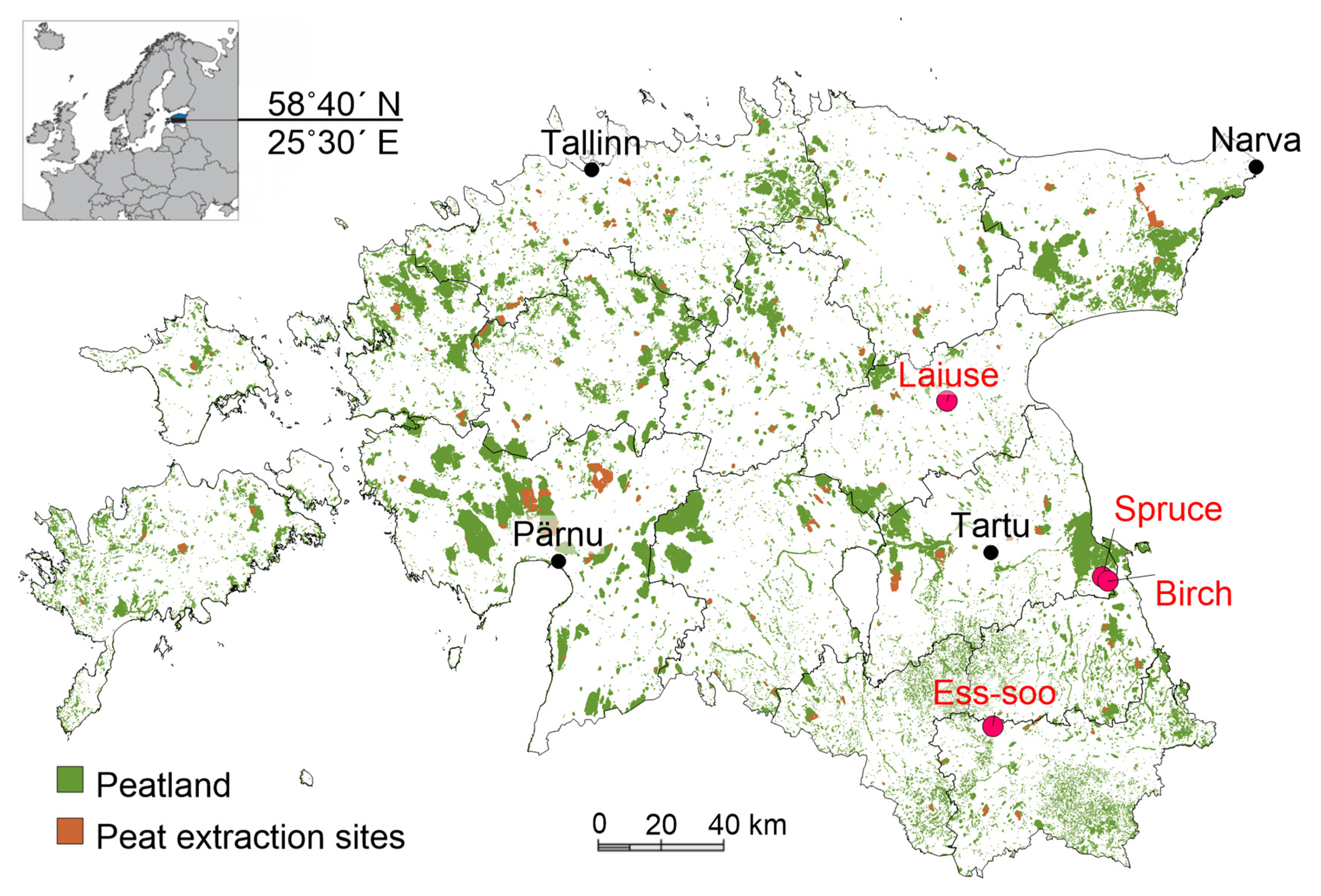
The study was conducted at two abandoned peat extraction areas (APEAs) and two drained peatland forests (DPFs) in eastern and southeastern Estonia. The locations of the study sites are shown in Figure 1.
From October 2014 until April 2019, we measured greenhouse gas fluxes (using the static chamber method) at two DPFs in Järvselja, eastern Estonia: a Downy birch (Betula pubescens Ehrh.) (DB) forest (58°17′22″ N, 27°19′2″ E) and a Norway spruce (Picea abies (L.) H. Karst.) (NS) forest (58°18′11″ N, 27°17′14″ E), both in Oxalis-type drained peatlands with two replicate plots (see forest stand parameters in Supplementary Table S1). Peat depth was more than 50 cm. In all 4 study plots, drainage work had been carried out in the early 1970s. From October 2017 until April 2019, we measured greenhouse gas fluxes in two APEAs: Ess-soo (ES) and Laiuse (LA). At Ess-soo (57°54′53″ N, 26°41′51″ E) the replicate plots were on adjacent peat fields which were separated by ditches. The peat fields had a slightly convex surface, without trees. Hare’s-tail cottongrass (Eriophorum vaginatum L.) coverage was 10 to 20%. At Laiuse (58°47′26″ N, 26°31′45″ E), the two plots were on adjacent peat fields which were separated by ditches. The most dominant plant species were E. vaginatum and bog haircap moss (Polytrichum strictum Bridel, J. Bot. (Schrader)). Pine and birch trees grew sparsely at the study site.
Both the Ess-soo and Laiuse sites are representative of Estonia’s APEAs, and the Norway spruce and Downy birch sites are typical drained forests in Estonia’s DPFs.
2.2. Meteorological Data
The meteorological analyses were based on air temperature measured hourly and calculated daily, as well as daily, monthly and annual precipitation from the Tartu Meteorological Station (58°15′51″ N, 26°27′41″ E), corresponding to weather conditions at the Downy birch study site (50 km from the station) and at the Norway spruce study site (48.5 km from the station); from the Jõgeva Meteorology Station (58°44′59″ N, 26°24′54″ E), corresponding to weather conditions at the Laiuse study site (8 km from the station); from Võru Meteorology Station (57°50′47″ N, 27°01′10″ E), corresponding to weather conditions at the Ess-soo study site (20 km from the station) (Table 1, Supplementary Figure S1).
2.3. Field Measurements
The static closed-chamber method [54] was used for the measurement of CO2, CH4 and N2O fluxes. Closed chambers (conical, made of polyvinyl chloride (PVC), height—50 cm, Ø—50 cm, volume—65 L) were installed in four replicates per plot. The chambers were sealed with a water filled ring on the soil surface. In case there was snow cover, the chambers were placed on the snow. Snow was not removed inside the collars and the chambers were sealed as previously described. Gas sampling was carried out twice a month from October to April. Measurements consisted of five gas samples which were collected into previously evacuated 50 mL gas bottles for 1 h (at 0, 15, 30, 45 and 60 min). At each plot during each gas sampling session, the depth of groundwater table (cm) in the observation wells (Ø—50 mm, up to 1.5 m deep PVC) was determined, and the soil temperature was measured at four depths (10, 20, 30 and 40 cm) by a handheld Comet S0141 temperature logger with Pt1000TG8 sensors (Comet Systems Ltd., Rožnov pod Radhoštšem, Czech Republic). During each gas sampling session at each plot, groundwater parameters were measured from piezometers (pH, oxygen concentration, redox potential, temperature, electrical conductivity) by a handheld YSI Professional Plus Multiparameter Water Quality Instrument with a Quatro field cable (YSI Incorporated, Yellow Springs, OH, USA), and air and ground surface temperature by a handheld Comet S0141 temperature logger with Pt1000TG8 sensors (Comet Systems Ltd., Rožnov pod Radhoštšem, Czech Republic). In addition, at drained forests sites, the soil temperature (at 5 cm depth) was measured with temperature probes (model CS 107, Campbell Scientific Inc., Logan, UT, USA) and soil volumetric water content (VWC; depth—10 cm) was recorded with water content reflectometers (model CS615, Campbell Scientific Inc., Logan, UT, USA) at each plot. The automated abiotic data were stored as 1-h averages on a data logger (CR1000, Campbell Scientific Inc., Logan, UT, USA).
2.4. Soil Analyses
For soil analyses, 3 composite samples from LA, DB and NS and 8 composite samples from ES were analyzed, and each sample consisted of 24 sub-samples at the LA and ES sites and 3 sub-samples at the DB and NS sites (Table S2). The sub-samples were mixed and homogenized before laboratory analyses. In the homogenized soil samples, the content of dry matter, ash (3 h at 550 °C) and total C were estimated using a dry combustion method on a varioMAX CNS elemental analyzer (Elementar Analysensysteme GmbH, Langenselbold, Germany). The soil samples were also analyzed for total nitrogen according to Kjeldahl (Tecator ASN3313), NH4-N (Tecator ASN 65-32/84) and NO3-N (Tecator ASN 65-31/84). The ammonium lactate extractable solution, using the flame photometric method was applied to analyze the available K, Ca and Mg content (Tecator ASTN 9/84). The analyses were carried out at the Plant Biochemistry Laboratory of the Estonian University of Life Sciences.
2.5. Gas Analyses
The gas concentrations in the collected samples were determined using a Shimadzu GC-2014 gas chromatography system (Shimadzu GC-2014 with an electron capture detector, flame ionization detector, and Loftfield autosampler, Loftfield Analytics, Göttingen, Germany) at the laboratory of the Department of Geography, Institute of Ecology and Earth Sciences, University of Tartu, Estonia [55]. Emission rates for one plot were calculated as the average of five subsamples. Gas fluxes were calculated from the linear increase or decrease in gas concentration in each chamber with time, using a linear regression equation [56], and were corrected for air temperature according to the ideal gas equation. The following criteria were followed for quality control: R-squared (R2) p-value < 0.05, R2 > 0.77 (5 data points) or R2 > 0.9 (4 data points) for CO2 and R2 p-value < 0.1, R2 > 0.65 (5 data points) or R2 > 0.8 (4 data points) for N2O and CH4. To achieve this, one data point was deleted of necessary. In case the difference between the minimum and maximum was smaller than 20 ppm/ppb (ppm applies to CO2 and ppb to CH4 and N2O), the R2 value was not considered and the data were included in the analysis. In case of snow cover, the volume of chamber was recalculated considering snow depth and density.
The summer period data originated from the unpublished report (https://media.rmk.ee/files/Rakendusuuring%20lopparuanne:Kodusoometsad.pdf) [57].
For the comparison of the climate impact of GHGs, we calculated their global warming potential (GWP) according to the radiative forcing. In a 100-year timespan, the GWP for CH4 and N2O is correspondingly 28 and 296 times larger than that of the equivalent amount of CO2 [58].
2.6. Statistical Analyses
Principal component analysis (PCA) was performed on environmental parameters using the R package ade4 v. 1.7–15 [59]. Differences in PCA between the sites were evaluated using PERMANOVA with 9999 permutations. The pairwise comparisons were corrected with the Bonferroni method using the vegan v. 2.5–6 R package [60].
The normality of distributions was checked using the Shapiro–Wilk, Anderson–Darling, Kolmogorov–Smirnov, Lilliefors and Jarque–Bera tests. The distribution of gas data deviated from normal, and hence non-parametric tests were performed. The median, 25% and 75% percentile, and minimum and maximum values of variables are presented. We used the Kruskal–Wallis analysis of variance (ANOVA) test and Dunn’s multiple comparison test to check the significance of differences between gas fluxes for different land-use categories and between different years at each study site, and the Spearman rank correlation to analyze the relationship between GHG fluxes and environmental parameters. p values were considered statistically significant after Benjamin–Hochberg correction. Statistical analysis was carried out using Statistica and XLSTAT. The level of significance of p < 0.05 was accepted in all cases, except in evaluating CH4 and N2O flux regressions, when p < 0.1 was accepted.
3. Results
3.1. PCA Analysis
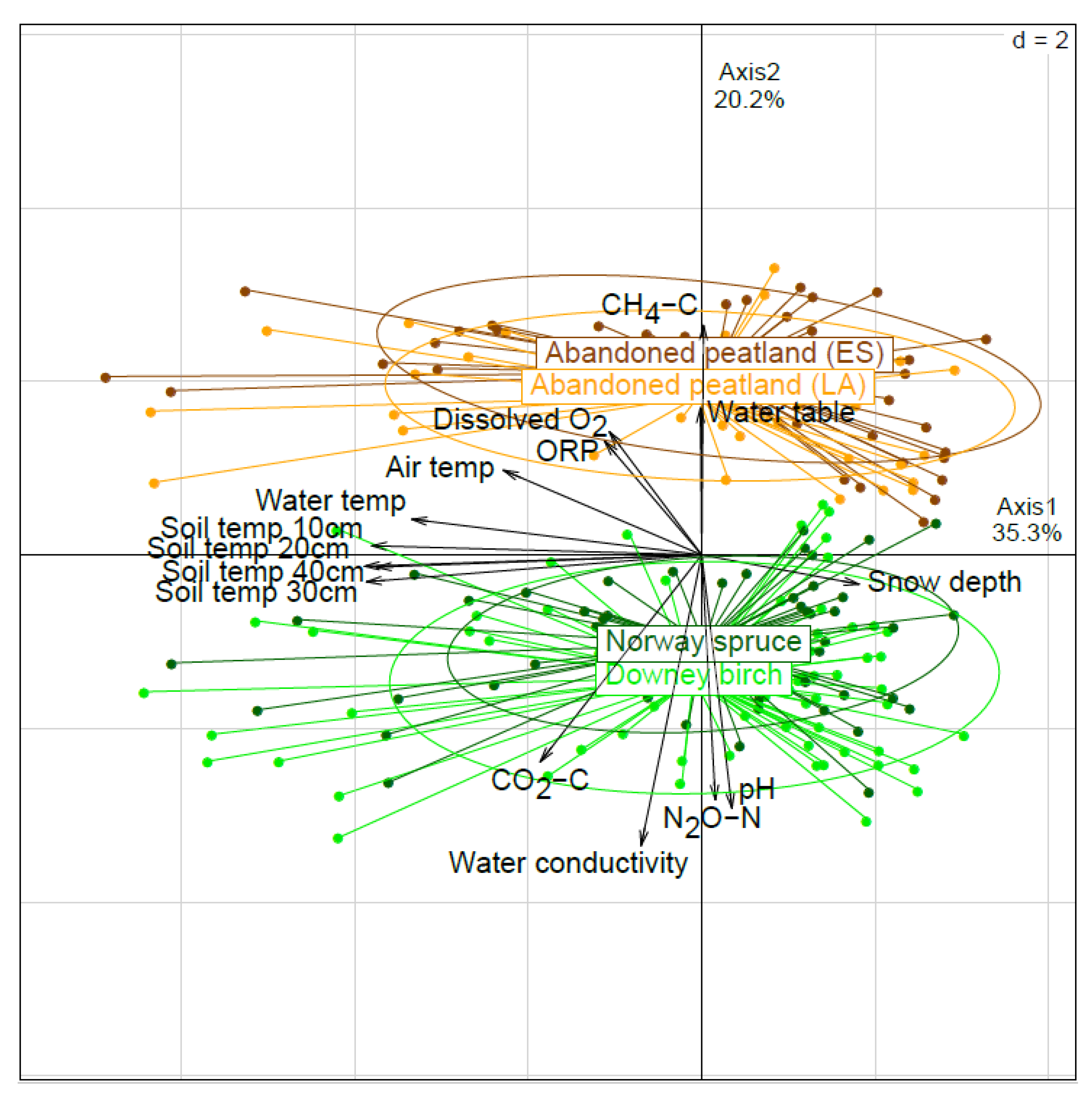
According to the principal component analysis (PCA) of the soil, water and gas emission characteristics, the APEAs (ES and LA) were under similar conditions and significantly different from peatland forests (DB and NS) (p < 0.001 in all comparisons), which were in turn similar to each other (Figure 2). The APEAs differed from the forests mainly in higher water table, dissolved O2 and oxidation-reduction potential (ORP) values, and in lower pH and water electrical conductivity. Different temperatures were strongly negatively related to snow depth, but they showed no significant difference between the studied sites. Considering the gas fluxes, the peatland forests were characterized by higher CO2-C and N2O-N, and lower CH4-C emissions compared to the APEAs.
More detailed relationships between the GHG fluxes and environmental characteristics were detected in the correlation analysis.
3.2. Soil CO2 Flux
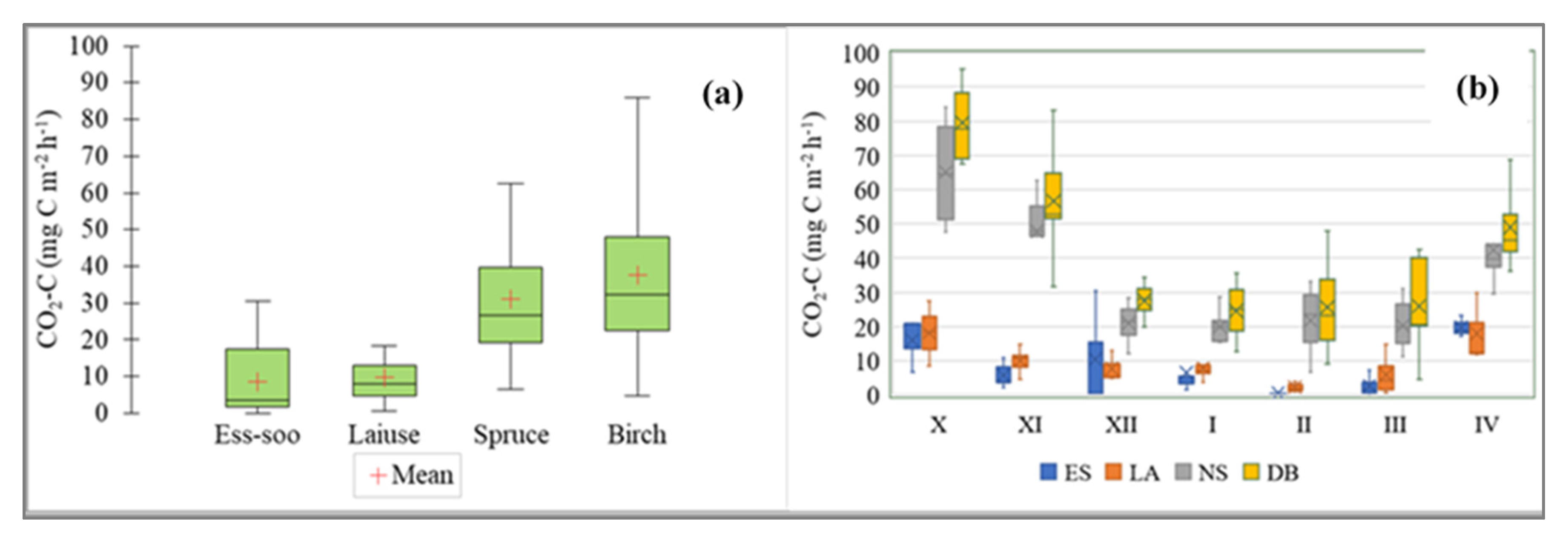
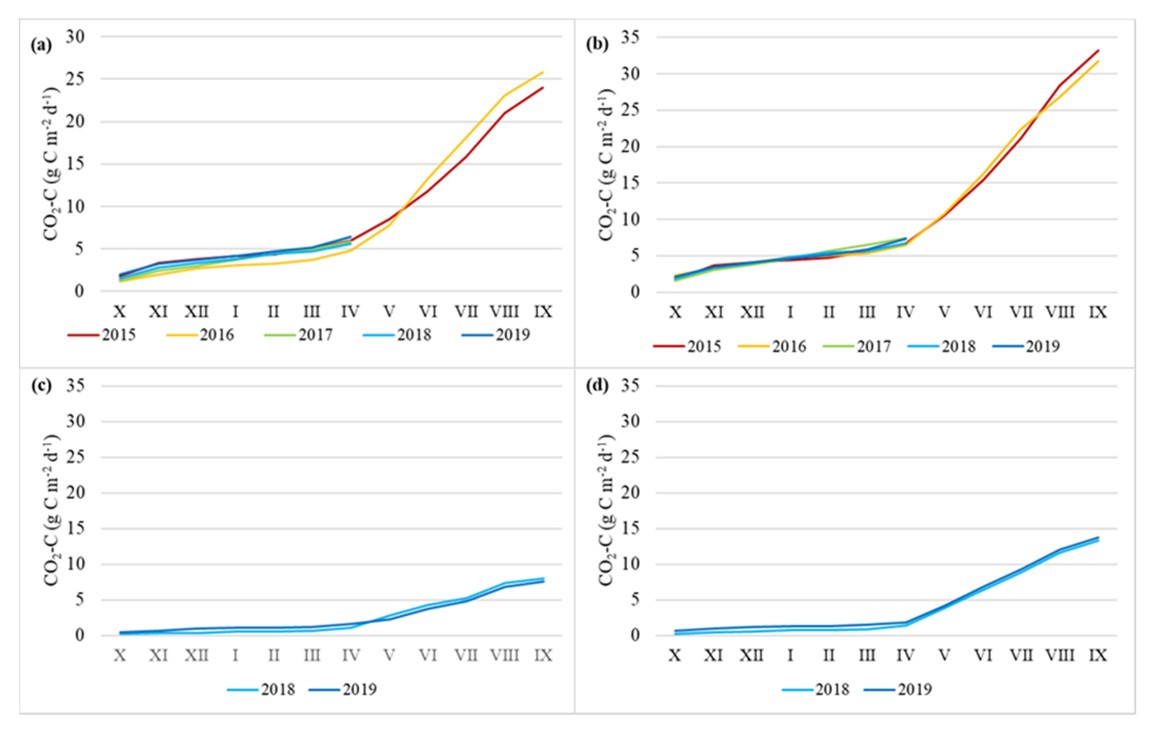
The daily average soil flux of carbon dioxide varied between −1.1 and 106 mg CO2-C m−2 h−1. The highest values were measured in October and April and the lowest values were measured in February (Figure 3). There was no significant difference between the four study sites (Kruskal–Wallis ANOVA test, multiple comparison of mean ranks). The median values of CO2-C fluxes were similar between the APEAs and DPFs, though the emissions were a little higher at the DPFs (Figure 3). There was no significant difference in CO2 fluxes between the years at any study site (Kruskal–Wallis ANOVA test) (Figure 4).
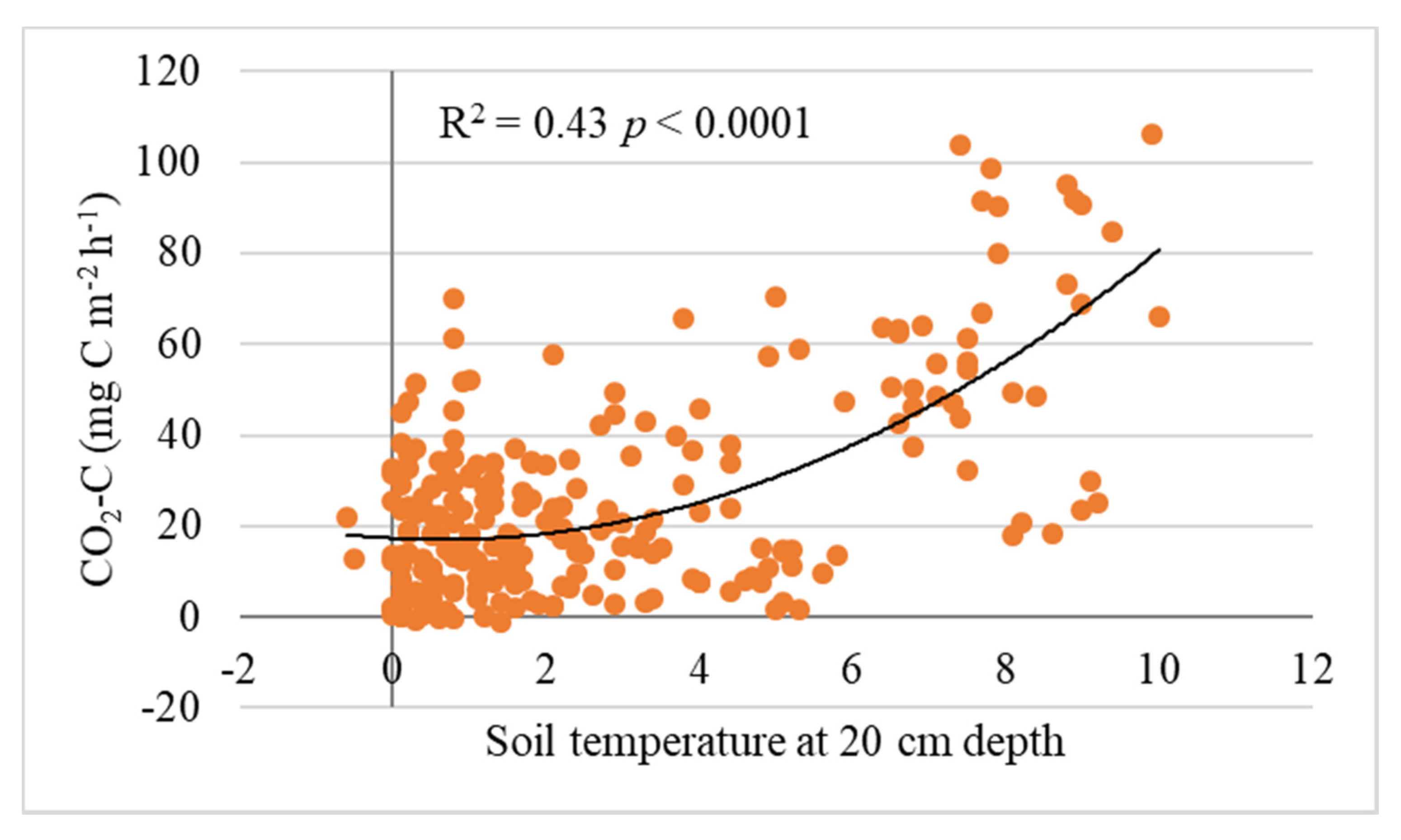
Across all study sites, the emissions correlated positively with soil temperature at all four depths (10, 20, 30 and 40 cm) (Figure 5) and air temperature (Table 2). The emissions correlated negatively with snow depth (Figure S2). In the DPFs, the correlations between CO2 flux and soil temperature (at 5, 10, 20, 30, and 40 cm depth) were stronger, and especially high in the Norway spruce forest (Table 2).
In the APEAs, at LA site the fluxes of CO2 showed a significantly positive correlation with redox potential (ORP) (Table 2). In the DPFs, the fluxes of CO2 were significantly and positively correlated with water temperature and pH (only in NS site; Table 2).
The fluxes of CO2 at the Downy birch DPF site showed a positive correlation with redox potential (ORP) and soil electrical conductivity.
The average values of cumulative winter half-year soil flux of CO2-C at the APEAs (ES and LA sites) and drained forests (NS and DB) were 47.8, 41.9, 159.8, and 194.7 g C m−2, respectively. The average winter-day fluxes were 199, 228, 761, 927 mg C m−2 d−1. Wintertime CO2 release from the APEAs (ES and LA sites) and drained forests (NS and DB) on average accounted for 18, 12, 21 and 20% of the total annual emission, respectively.
3.3. CH4 Fluxes
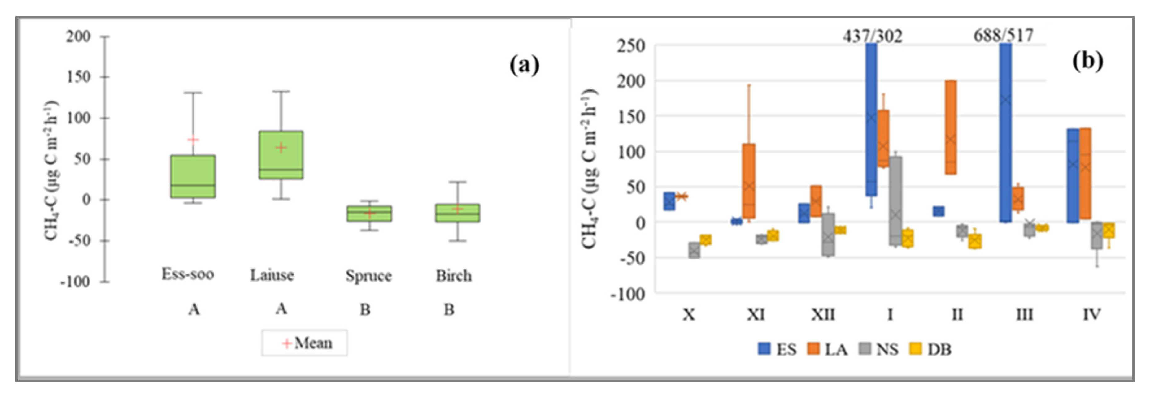
The average CH4-C emissions of varied between −97.7 and 1201.9 µg CH4-C m−2 h−1. There was a significant difference between the APEAs and DPFs (Kruskal–Wallis ANOVA test, multiple comparison of mean ranks; p < 0.05), with the highest amounts emitted from the APEAs (Figure 6). The negative values, which indicate methane consumption, were registered mainly from the DPFs. There was no clear temporal pattern, but in general, the fluxes were higher from October to January and lowest in February and March (Figure 6). There was no significant difference in the CH4 fluxes between the different years at the APEAs and the Norway Spruce site (Kruskal–Wallis ANOVA test) (Figure 7). CH4 fluxes in winters 2014/2015 and 2018/2019 showed statistically significant differences at the Downy birch DPF site (Kruskal–Wallis ANOVA test) (Figure 7).
At Laiuse APEA and the Norway spruce DPF site, the CH4 fluxes correlated positively with water table depth (Table 2). CH4 flux showed the highest values at a water table >20 cm below the surface (Figure S4). At the APEAs, the fluxes of CH4 showed a significant (p < 0.05) positive correlation with soil temperature at all four depths (10, 20, 30 and 40 cm; Table 2). The fluxes of CH4 showed a negative correlation with snow depth and a positive correlation with water table depth and water temperature at the Laiuse APEA site. The fluxes of CH4 showed a positive correlation with ground surface temperature and air temperature at the Ess-soo APEA site. In the drained forests, the fluxes of CH4 were significantly and negatively correlated with water temperature and soil temperature at all four depths (10, 20, 30 and 40 cm) (Table 2). At the NS site, CH4 correlated negatively with water electrical conductivity and positively with water table depth.
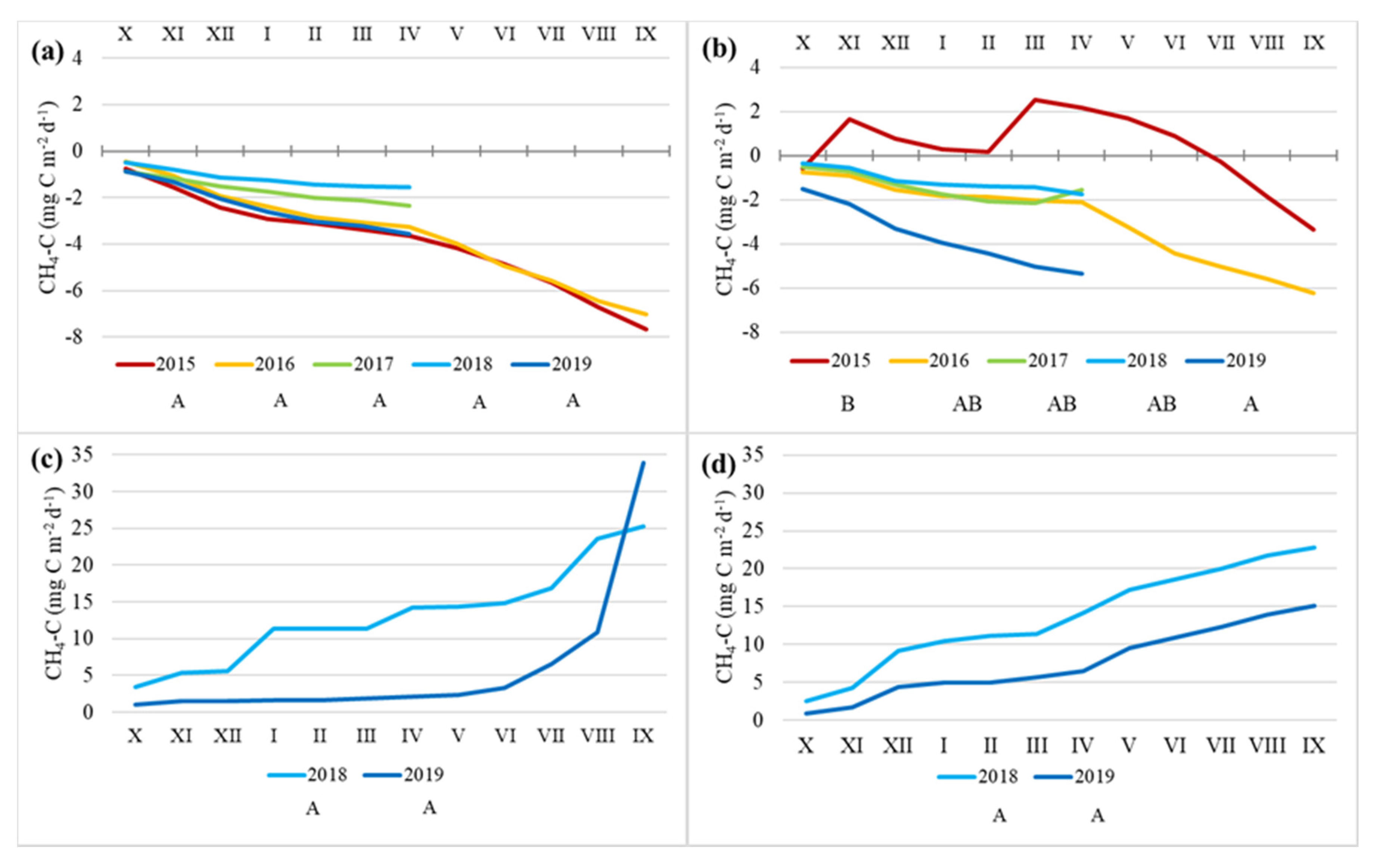
Average values of the cumulative winter half-year soil efflux of CH4-C in the abandoned peat extraction areas (the ES and LA sites) and drained forests (Spruce and Birch) were 0.25, 0.31, −0.11, and −0.07 g C m−2, respectively. Average winter-day emissions were 1175, 1471, −177, and −140 µg CH4-C m−2 d−1. Wintertime CH4 release from the APEAs (ES and LA site) on average accounted for 31 and 52% of the total annual emission, respectively, and wintertime atmospheric CH4 consumption in the drained forests (Spruce and Birch) on average accounted for 46 and (33%) of the total annual consumption, respectively. Even though in the birch forest methane consumption occurred in most winters, there was a slight methane release at the beginning and/or the end of winter (Figure 7b).
3.4. N2O Fluxes
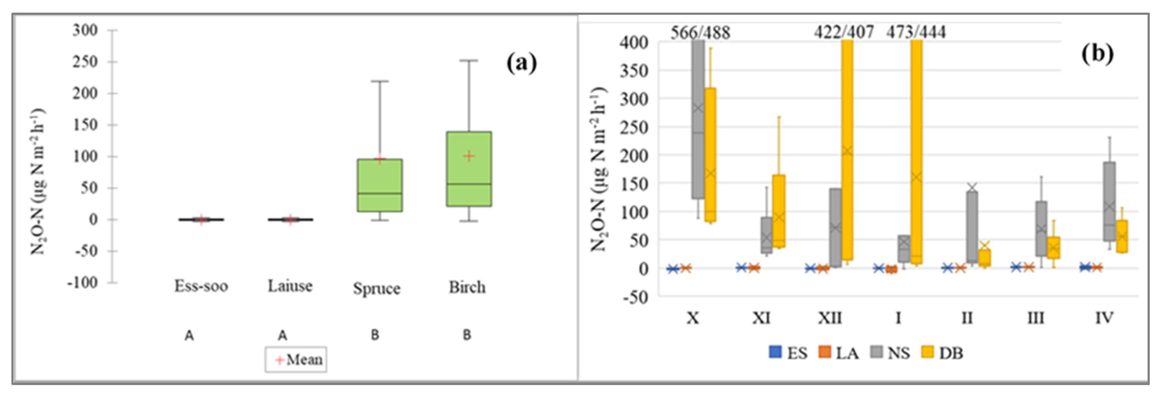
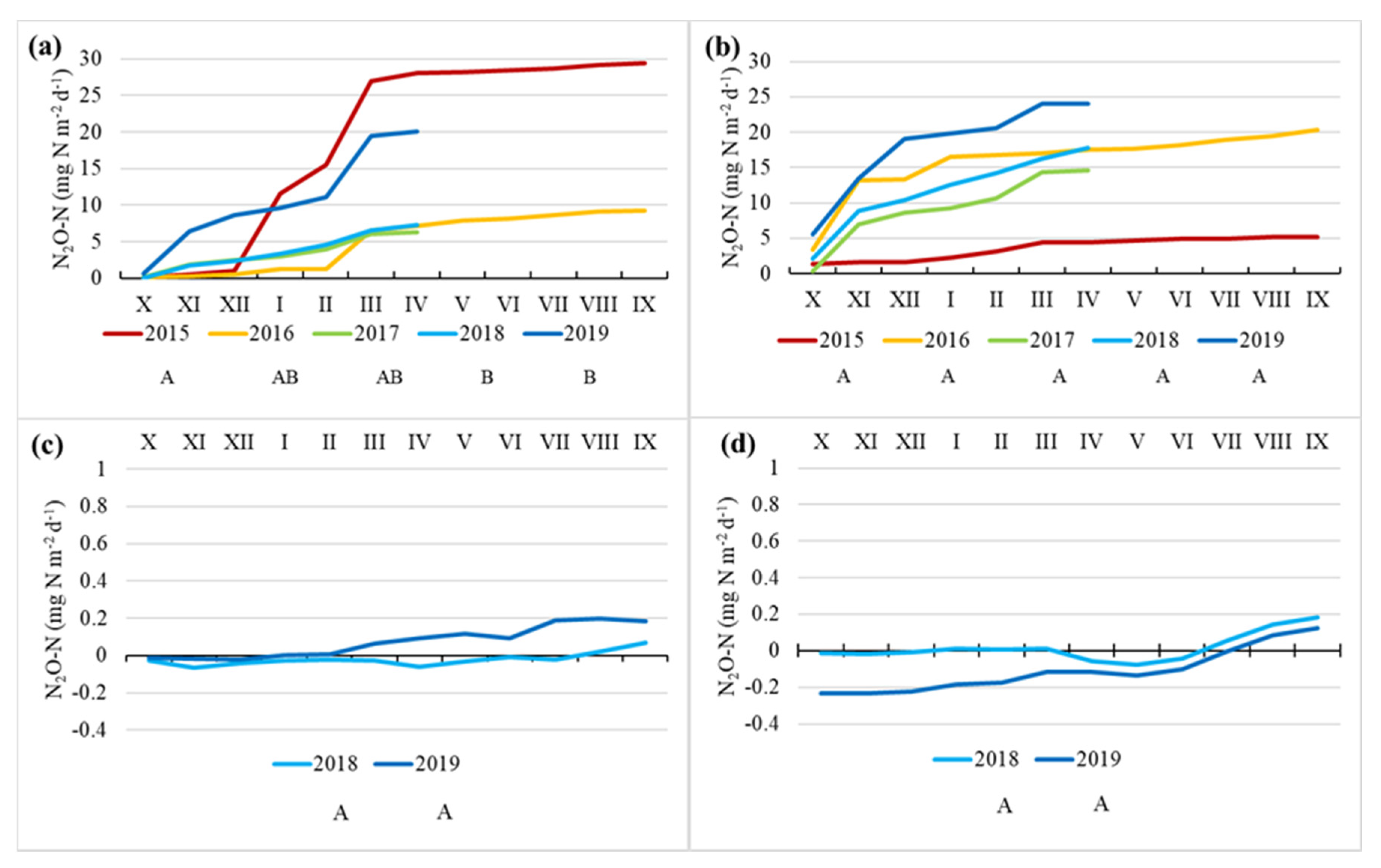
The average emissions of N2O-N varied between −32.2 and 1440.8 µg N2O-N m−2 h−1. There was a significant difference between the APEAs and DPFs (Kruskal–Wallis ANOVA test; multiple comparison of mean ranks; p < 0.05; Figure 8); the highest emissions in N2O fluxes between the years at the APEAs and Downy birch DPF site (Kruskal–Wallis ANOVA test; Figure 9). N2O fluxes in the 2014/2015 winter differed significantly from fluxes at the Norway spruce DPF site in the 2017/2018 and 2018/2019 winters (Kruskal–Wallis ANOVA test) (Figure 8). The highest peaks were registered in November and March, when freeze–thaw events were most common (Figure 9).
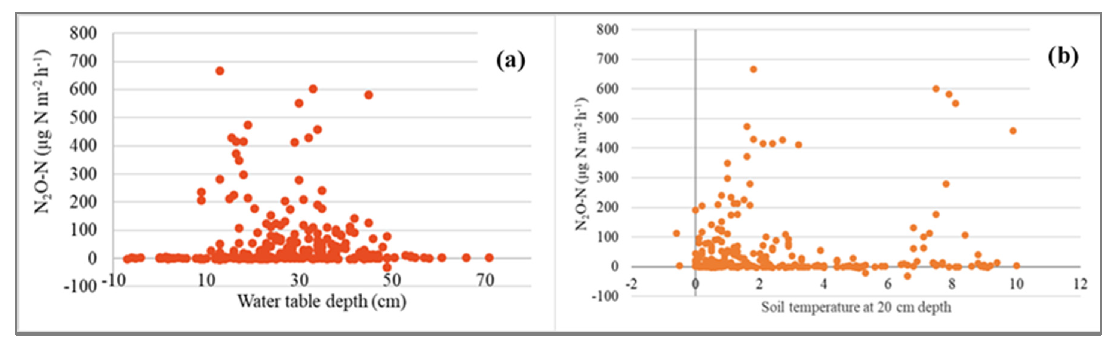
Across all sites, emissions of N2O correlated negatively with water table depth. Thus, the highest N2O fluxes were observed at a water table depth of from −30 to −40 cm (Figure 10a). The N2O emission showed high values at soil temperatures around 0 °C and 8 °C (Figure 10b). N2O fluxes at the ES and LA sites were negatively correlated with air temperature. At the ES site, the N2O fluxes correlated negatively with soil temperature at all four depths (10, 20, 30 and 40 cm), ground surface temperature, ORP, water table depth and water temperature. The fluxes of N2O had positive correlation with snow depth at the Ess-soo APEA site (Table 2).
In the spruce forest, the fluxes of N2O were positively correlated with water electrical conductivity and water table depth, and negatively correlated with soil temperature at 10 and 30 cm depth (Table 2).
The average values of the cumulative winter half-year soil efflux of N2O-N at the APEAs (ES and LA sites) and DPFs (the Norway spruce and Downy birch sites) were 0.0005, −0.003, 0.4, and 0.4 g N m−2, respectively. The average winter-day emissions of N2O 2.38, −12.1, 2000, and 2001 µg N2O-N m−2 d−1. Wintertime N2O release from the Norway spruce and Downy birch DPF sites accounted for 87 and 87% of the total annual emission, respectively.
4. Discussion
4.1. Differences in Peat Layer and Environmental Factors
There was a significant difference in peat parameters between the APEAs and DPFs (Figure 2). The top layer of peat had been removed from the peat extraction areas. The remaining peat layer consisted of compacted peat with likely recalcitrant organic carbon. Meanwhile, in the drained forests, only drainage had been conducted and no soil was removed. The most acidic soil occurred in the APEAs (especially the Ess-soo site), while the DPFs were the most neutral (pH values: 2.5, 3.0, 3.8, 4.0; in the Ess-soo and Laiuse APEAs and the Downy birch and Norway spruce DPFs, respectively). There were also significant differences in C/N ratio, which was considerably higher in the APEAs and lower in the DPFs: 45, 68, 15 and 19 in the Ess-soo, Laiuse, Downy birch and Norway spruce sites, respectively. Similarly, environmental factors such as precipitation, soil moisture, groundwater depth, air and soil temperature varied between the sites. These differences were crucial in the formation of the GHG fluxes in the sites (Appendix A).
4.2. Soil CO2 Fluxes
Average estimated wintertime CO2-C losses from the APEAs and drained forests were 42–48 and 169–195 g CO2-C m−2, respectively. Wintertime CO2 efflux made up 10–25% of the annual release. This is similar to findings in earlier works, where wintertime CO2 fluxes have been estimated. The share of wintertime CO2 from annual respiration in a drained peatland forest was 21% [5], in a boreal agricultural peat soil 23% [36], in a minerotrophic fen 25% [61] and from a boreal forest 20% [31]. In general, winter CO2 emissions in temperate and boreal areas are in the range of 10 to 40% [61]. In Arctic areas with more than 200 days of snow cover, winter CO2 emissions are 10–30% of annual soil respiration [31]. The variation can be due to different soil types and ecosystems. In our study, the emission and percentage from annual release was higher in the DPFs and lower in the APEAs with sparse vegetation.
Our results closely correspond with those of other studies in which CO2 fluxes were well explained by air temperature and soil temperature [5,31,35,36,47,62]. Kim and Kodama [31] found strong correlation between wintertime CO2 flux and air temperature. Lohila et al. [36] have suggested that air temperature is the most important component that influences CO2 efflux throughout the whole year. Our results showed a slightly stronger correlation with upper layer soil temperatures than air temperature.
The correlations between CO2 emission and air and soil temperatures were stronger in drained forests. In all areas, the correlation was strongest with the topsoil (5–10 cm) temperatures and lower with deeper (40 cm) soil temperatures.
Waddington et al. [63] have pointed out the importance of the top layer (50 cm) of peat in CO2 production of peatlands, as this has higher substrate quality due to its proximity to organic matter inputs and better access to oxygen. This may also explain why in the APEAs (ES, LA) CO2-C emissions were lower in comparison with drained forests—Sphagnum moss had been removed from the sites and the area was covered with sparse vegetation. Though at the LA site there were more vegetation, the average water level was also higher (party flooded in spring during snow melt). Due to the high water level, the circumstances were unfavorable for further peat oxidation, which resulted in lower soil CO2 efflux compared to the ES site. In both APEAs, the easier biodegradable upper layers of peat had been removed and the remaining deeper layers likely consisted of recalcitrant peat, which was not favorable for CO2 production [64,65].
There was no clear relationship between CO2-C efflux and water level (Figure S3). A significant difference in water table depth was found between the LA site and other sites (Kruskal–Wallis analysis of variance (ANOVA) test and Dunn’s multiple comparison test, p < 0.01). The LA site was slightly flooded in springtime, up to 7 cm above the ground.
CO2 measurement in the presence of snow always provides challenges, especially in warming climate conditions [66]. Negative correlation with snow depth was found in all study sites (not statistically significant at ES site). The correlation with snow depth was stronger in the DPFs and especially high in one Downy birch forest microsite (R2 = −0.75, p < 0.001). Soil temperature, which is affected by the thickness of snow and air-temperature, regulates the activity of microbes, which determine the amount of CO2 flux from the soil [35]. If the ground is covered with snow, especially with deep snow, then the soils are wetter and warmer, which can increase heterotrophic respiration. In the case of less snow, the soils could freeze more deeply and result in lower CO2 emissions. However, thin and sporadic snow cover may cause higher frequency of freeze–thaw events and winter CO2 emissions could be larger with a warmer climate [67]. On the one hand, temporary ice cover formed on snow-free soil patches may store CO2 in soil and degassing after soil is warming and ice is thawing [68], while on the other hand, freeze–thaw events may increase the soil-dissolved organic carbon (DOC) and dissolved organic nitrogen (DON) concentration [69] and, consequently, intensify the activity of soil decomposers [70] and GHG emission. The disturbance of fine roots can be a source for fresh available carbon for microorganisms [71,72]. Dense woody root mats in drained peatland forest sites (Table S1) are likely a reason why the CO2 flux was higher here than that in the APEAs without any remarkable plant root system.
Stielstra et al. [52] found that soil moisture is the primary determinant of carbon fluxes in seasonally snow-covered forest ecosystems. In this study, a weak positive correlation between CO2 flux and soil moisture was found only in the spruce forest (NS).
At the APEAs, CO2 consumption was registered in few measuring times. Generally, CO2 flux is not negative out of the growing season. However, some studies showed that many evergreen plants and mosses maintain their photosynthetic activity throughout the winter [73,74,75]. This factor of CO2 consumption can play a role in DPFs but not in APEAs with scarce vegetation.
4.3. CH4 Fluxes
Average estimated wintertime CH4-C emissions from the APEAs and drained forests were 0.25–0.31 and −0.11–−0.07 g CH4-C m−2, respectively. Wintertime CH4 fluxes made up 31–52% of annual release at the APEAs and 33–49% of annual consumption in the drained forests. Average daily CH4 fluxes from the APEAs were 1.2–1.5 mg CH4-C m−2 d−1. Compared to previous studies in Minnesota peatlands, the emissions were lower (3–16 mg CH4 m−2 d−1) [12]. However, wintertime fluxes made up 11–21% of annual emissions in the Minnesota peatlands, which is lower than our results. Our drained forests were annual sinks of CH4. This result corresponds well with earlier studies [76,77]. In the forest, the water table is relatively low due to canopy interception of precipitation and evapotranspiration [78], which may lead to a soil sink of CH4 [76,77].
CH4 consumption in our drained forests correlated negatively with soil temperature (strongest correlation with soil temperature at 20–40 cm) and positively with water level depth. Meanwhile, in our APEAs, the emissions of CH4 correlated positively with air, water and soil temperature and water table depth. Low soil temperature slowed down CH4 production in the APEAs, which is in accordance with earlier studies [5,13]. A part of methane emission in our APEAs was likely caused by the release of capped CH4 from frozen surface layers: emission peaks occurred mostly when peat surface was slightly frozen. The fluxes were lower in mid-winter when snow cover was at its deepest. In Laiuse APEA, a significant correlation between CH4 flux and snow depth was found.
4.4. N2O Fluxes
Average values of cumulative winter half-year soil N2O-N flux in the APEAs (ES and LA) and drained forests (spruce and birch) were 0.0005, −0.003, 0.4, and 0.4 g N m−2, respectively. Average winter-day emissions of N2O were 2.38, −12.1, 2000, and 2001 µg N2O-N m−2 d−1. Wintertime N2O release from the drained forests (spruce and birch) accounted for 87% of the total annual emission in both sites. The N2O fluxes were influenced by soil properties, the ecosystem and the weather. No strong relationship was found between N2O emission rates and soil factors such as soil moisture (no correlation) and soil temperature (weak correlation). This result corresponds well with Flessa et al. [40]. The highest peaks of N2O emission occurred during freeze–thaw events. The months with the highest emissions were November and March. The high N2O peaks during the freeze–thaw events can be explained by a release of organic carbon as energy source for denitrification, by decomposing soil aggregates and killing soil organisms [10,33]. In the snowy winters, the N2O emissions were especially high in November and March. In mild winters with a thin snow cover or no snow at all, the emissions were higher also in mid-winter. In contrast, Brooks et al. [79] found that wintertime N2O fluxes were higher in the winters when snow cover formed earlier and lasted longer. Like Pärn et al. [80], who found an optimal range of soil water content for N2O emissions from organic soils, our study shows an intermediate water table depth (20–40 cm) at which the emission was highest (Figure 10a). The components of the determination of wintertime GWP were different for the APEAs and DBFs. In the DPFs, the flux of N2O was the main component, showing 3–6 times higher values than that of the CO2 flux, while the role of CH4 was of little importance. In the APEAs, CO2 and CH4 made up almost equal parts, whereas the impact of N2O on global warming was minor. In none of the study sites the slight consumption of CH4 could compensate the GWP from CO2 and N2O emissions.
5. Conclusions
Wintertime CO2 and N2O fluxes in the DPFs were significantly higher than those from the APEAs. Vice versa, the mean CH4 fluxes from the DPFs showed a cumulative consumption in the drained forests, whereas in the APEAs, emission dominated. Our hypotheses on snow cover effect was only partly supported, showing both a positive and negative impact on different sites and gases. In general, thin and scattered snow cover during the freeze–thaw periods initiates GHG fluxes. In our study, the winters were relatively mild and snow cover was rather thin. Across all study sites, CO2 flux correlated positively with soil and ground and air temperature. A continuous snow depth of >5 cm did not influence CO2, while under no snow or thin snow fluxes showed the largest variation. Regarding the N2O and CH4 fluxes, the correlation with snow depth varied between the gases and sites: in the APEAs and the spruce forest, snow cover slightly increased N2O flux, while CH4 emission in the APEAs showed a negative correlation with snow depth. Most likely due to the freeze–thaw effect, the highest N2O emissions appeared at soil temperatures of around 0 °C, whereas the fluxes correlated negatively with soil temperature.
As a well-known phenomenon from previous studies, the highest N2O fluxes were observed at an intermediate water table depth of −30 to −40 cm, which corresponds with the optimal soil moisture level for microbial activity in the soil matrix.
Considering the global warming potential (GWP) of the greenhouse gas emissions from DPFs during the winters, the flux of N2O (GWP 265 times CO2 equivalent) was the main component, showing 3–6 times higher values than that of the CO2 flux, while the role of CH4 (GWP 28 times CO2 equivalent) was of little importance. In the APEAs, CO2 and CH4 made up almost equal parts, whereas the impact of N2O on global warming was minor.
In northern regions, milder winters are becoming more frequent due to the climate warming. An increase in freeze–thaw cycles will increase the likelihood of wintertime GHG emissions, especially from DPFs. Groundwater regulation around high levels in these areas would mitigate the emissions. Further analyses must focus on this and other possible measures to mitigate GHG fluxes from disturbed peatland systems. Our results might also be useful for the development of the GHG-based functional classification of soils [81].
Supplementary Materials
The following materials are available online at https://www.mdpi.com/2073-4433/11/7/731/s1, Table S1. Forest survey data in the Downy birch and Norway spruce sites. Average values are shown. Table S2. Soil physical-chemical parameters: Drained peatland forests—Downy birch (DB); Norway spruce (NS). Abandoned peat production areas: Ess-soo (ES), Laiuse (LA). Figure S1: Mean monthly precipitation (mm) (left) and monthly air temperature (°C) (right) at Jõgeva (corresponding to Laiuse study site), Tartu–Tõravere (corresponding to the Spruce and Birch forest study sites) and Võru weather stations (corresponding to the Ess-soo study site) in the period of 2015–2019. Figure S2: The relationship between CO2-C efflux and snow depth (cm) at all study sites. Figure S3: The relationship between CO2-C efflux and water table depth (cm) at all study sites. Negative water table depth values show that the surface was flooded. Figure S4: The relationship between CH4-C emissions and water table depth (cm) at all study sites. Negative water table depth values show that the surface was flooded.
Author Contributions
Conceptualization, Ü.M., B.V., J.J.; methodology, Ü.M., A.K., M.M. (Martin Maddison), M.E., A.T., G.V.; software, M.E.; validation, Ü.M., B.V., A.K., M.E.; formal analysis, Ü.M., B.V., A.K., A.T.; investigation, B.V., A.T., M.M. (Mart Muhel), M.M. (Martin Maddison), G.V., A.K.; resources, Ü.M.; data curation, B.V., Ü.M., A.K., M.E.; writing—original draft preparation, B.V., Ü.M.; writing—review and editing, B.V., Ü.M., A.K., M.E., J.J.; visualization, B.V., M.E.; supervision, Ü.M., J.J.; project administration, Ü.M., J.J.; funding acquisition, Ü.M., A.K. All authors have read and agreed to the published version of the manuscript.
Funding
This study was supported by the Estonian Research Council (IUT2-16 and PRG352); the EU through the European Regional Development Fund (Centre of Excellence EcolChange, Estonia) and by the Estonian State Forest Management Centre (projects LLOOM13056 “Carbon and nitrogen cycling in forests with altered water regime “, 2013–2016 and LLTOM17250 “Water level restoration in cut-away peatlands: development of integrated monitoring methods and monitoring”, 2017–2023).
Acknowledgments
We thank Jaan Pärn for the copyediting.
Conflicts of Interest
The authors declare no conflict of interest.
Appendix A
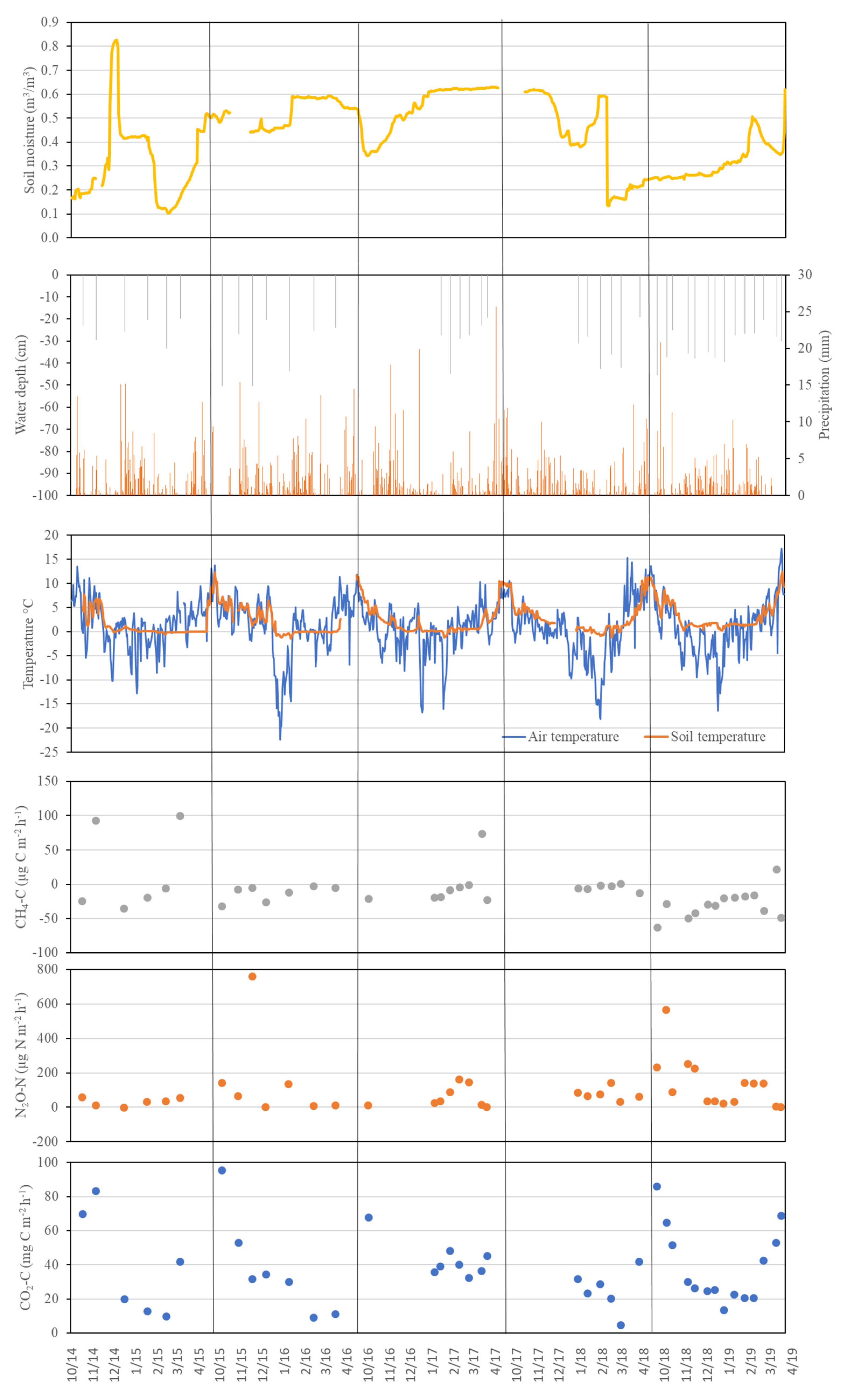
Figure A1.
Temporal dynamics of key environmental parameters and greenhouse gas emissions in the Downy birch forest (DB).
Figure A1.
Temporal dynamics of key environmental parameters and greenhouse gas emissions in the Downy birch forest (DB).

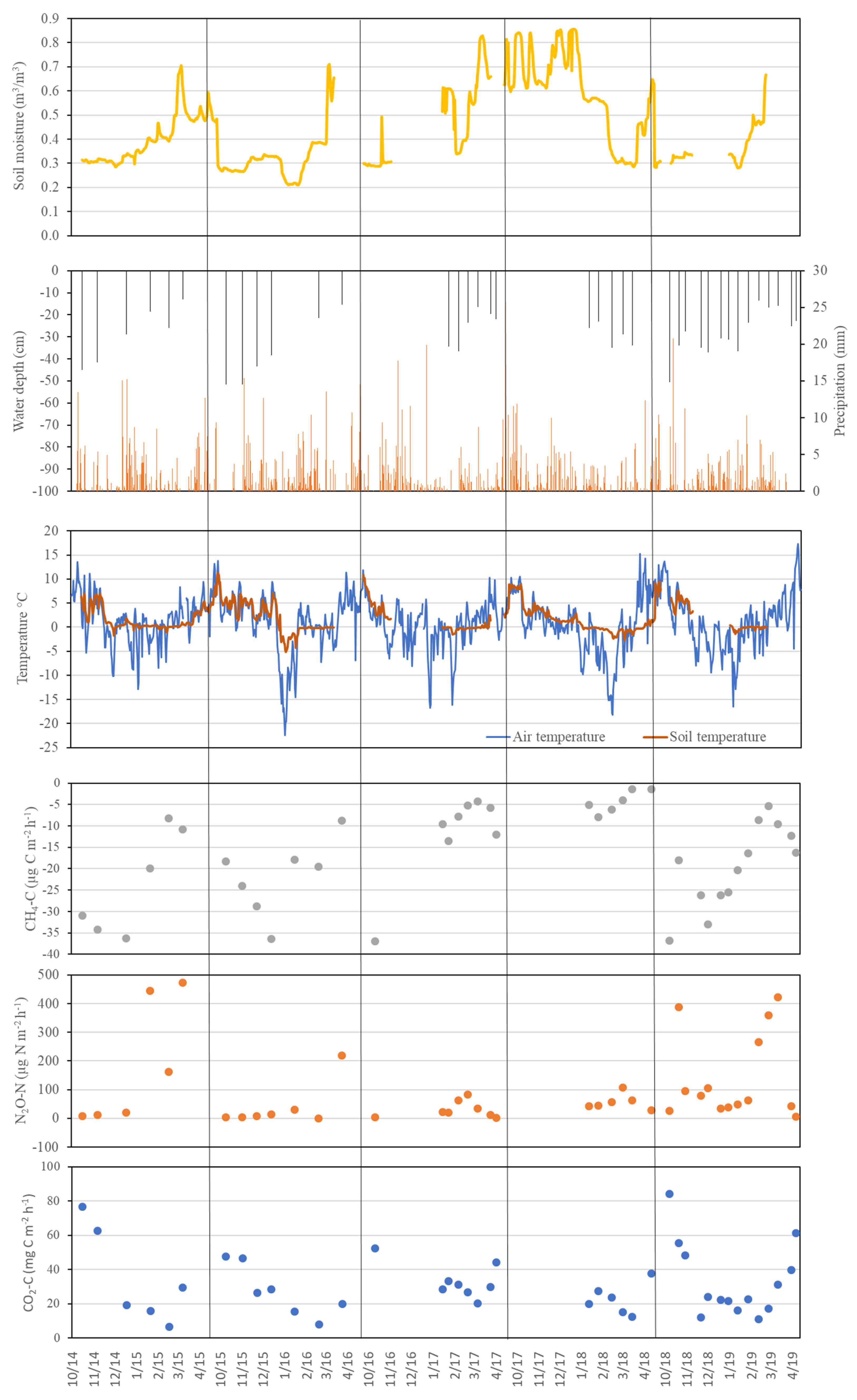
Figure A2.
Temporal dynamics of key environmental parameters and greenhouse gas emissions in the Norway spruce forest (NS).
Figure A2.
Temporal dynamics of key environmental parameters and greenhouse gas emissions in the Norway spruce forest (NS).

References
- WMO Greenhouse Gas Bulletin; WMO: Geneva, Switzerland, 2019; p. 8.
- Sommerfeld, R.A.; Mosier, A.R.; Musselman, R.C. CO2, CH4 and N2O flux through a Wyoming snowpack and implications for global budgets. Nature 1993, 361, 140–142. [Google Scholar] [CrossRef]
- Winston, G.C.; Sundquist, E.T.; Stephens, B.B.; Trumbore, S.E. Winter CO2 fluxes in a boreal forest. J. Geophys. Res.-Atmos. 1997, 102, 28795–28804. [Google Scholar] [CrossRef] [Green Version]
- Mast, M.A.; Wickland, K.P.; Striegl, R.T.; Clow, D.W. Winter fluxes of CO2 and CH4 from subalpine soils in Rocky Mountain National Park, Colorado. Glob. Biogeochem. Cycles 1998, 12, 607–620. [Google Scholar] [CrossRef]
- Alm, J.; Saarnio, S.; Nykänen, H.; Silvola, J.; Martikainen, P. Winter CO2, CH4 and N2O fluxes on some natural and drained boreal peatlands. Biogeochemistry 1999, 44, 163–186. [Google Scholar] [CrossRef]
- Fahnestock, J.T.; Jones, M.H.; Welker, J.M. Wintertime CO2 efflux from Arctic soils: Implications for annual carbon budgets. Glob. Biogeochem. Cycles 1999, 13, 775–779. [Google Scholar] [CrossRef]
- Groffman, P.M.; Hardy, J.P.; Driscoll, C.T.; Fahey, T.J. Snow depth, soil freezing, and fluxes of carbon dioxide, nitrous oxide and methane in a northern hardwood forest. Glob. Chang. Biol. 2006, 12, 1748–1760. [Google Scholar] [CrossRef] [Green Version]
- Maljanen, M.; Kohonen, A.-R.; Virkajärvi, P.; Martikainen, P.J. Fluxes and production of N2O, CO2 and CH4 in boreal agricultural soil during winter as affected by snow cover. Tellus Ser. B-Chem. Phys. Meteorol. 2007, 59, 853–859. [Google Scholar] [CrossRef] [Green Version]
- Kim, Y.; Tsunogai, S.; Tanaka, N. Winter CO2 emission and its production rate in cold temperate soils of northern Japan: 222Rn as a proxy for the validation of CO2 diffusivity. Polar Sci. 2019, 22, 100480. [Google Scholar] [CrossRef]
- Hao, Q.J.; Wang, Y.S.; Song, C.C.; Huang, Y. Contribution of winter fluxes to the annual CH4, CO2 and N2O emissions from freshwater marshes in the Sanjiang Plain. J. Environ. Sci. 2006, 18, 270–275. [Google Scholar]
- Kim, Y.; Ueyama, M.; Nakagawa, F.; Tsunogai, U.; Harazono, Y.; Tanaka, N. Assessment of winter fluxes of CO2 and CH4 in boreal forest soils of central Alaska estimated by the profile method and the chamber method: A diagnosis of methane emission and implications for the regional carbon budget. Tellus B Chem. Phys. Meteorol. 2007, 59, 223–233. [Google Scholar] [CrossRef]
- Dise, N. Winter Fluxes of Methane from Minnesota Peatlands. Biogeochemistry 1992, 17, 71–83. [Google Scholar] [CrossRef]
- Melloh, R.A.; Crill, P.M. Winter methane dynamics in a temperate peatland. Glob. Biogeochem. Cycles 1996, 10, 247–254. [Google Scholar] [CrossRef]
- Panikov, N.S.; Dedysh, S.N. Cold season CH4 and CO2 emission from boreal peat bogs (West Siberia): Winter fluxes and thaw activation dynamics. Glob. Biogeochem. Cycles 2000, 14, 1071–1080. [Google Scholar] [CrossRef]
- Jiang, C.; Wang, Y.; Hao, Q.; Song, C. Effect of land-use change on CH4 and N2O emissions from freshwater marsh in Northeast China. Atmos. Environ. 2009, 43, 3305–3309. [Google Scholar] [CrossRef]
- Koch, O.; Tscherko, D.; Kandeler, E. Seasonal and diurnal net methane emissions from organic soils of the Eastern Alps, Austria: Effects of soil temperature, water balance, and plant biomass. Arct. Antarct. Alp. Res. 2007, 39, 438–448. [Google Scholar] [CrossRef] [Green Version]
- Miao, Y.; Song, C.; Wang, X.; Meng, H.; Sun, L.; Wang, J. Annual Carbon Gas Emissions from a Boreal Peatland in Continuous Permafrost Zone, Northeast China. Clean-Soil Air Water 2016, 44, 456–463. [Google Scholar] [CrossRef]
- Nykänen, H.; Alm, J.; Lång, K.; Silvola, J.; Martikainen, P.J. Emissions of CH4, N2O and CO2 from a virgin fen and a fen drained for grassland in Finland. J. Biogeogr. 1995, 22, 351–357. [Google Scholar] [CrossRef]
- Song, W.; Wang, H.; Wang, G.; Chen, L.; Jin, Z.; Zhuang, Q.; He, J.-S. Methane emissions from an alpine wetland on the Tibetan Plateau: Neglected but vital contribution of the nongrowing season. J. Geophys. Res.-Biogeosci. 2015, 120, 1475–1490. [Google Scholar] [CrossRef]
- Kammann, C.; Grunhage, L.; Muller, C.; Jacobi, S.; Jager, H.J. Seasonal variability and mitigation options for N2O emissions from differently managed grasslands. Environ. Pollut. 1998, 102, 179–186. [Google Scholar] [CrossRef]
- Kim, Y.; Tanaka, N. Winter N2O emission rate and its production rate in soil underlying the snowpack in a subboreal region, Japan. J. Geophys. Res.-Atmos. 2002, 107, 4406. [Google Scholar] [CrossRef]
- Maljanen, M.; Hytönen, J.; Martikainen, P.J. Fluxes of N2O, CH4 and CO2 on afforested boreal agricultural soils. Plant Soil 2001, 231, 113–121. [Google Scholar] [CrossRef]
- Maljanen, M.; Komulainen, V.M.; Hytönen, J.; Martikainen, P.; Laine, J. Carbon dioxide, nitrous oxide and methane dynamics in boreal organic agricultural soils with different soil characteristics. Soil Biol. Biochem. 2004, 36, 1801–1808. [Google Scholar] [CrossRef]
- Papen, H.; Butterbach-Bahl, K. A 3-year continuous record of nitrogen trace gas fluxes from untreated and limed soil of a N-saturated spruce and beech forest ecosystem in Germany: 1. N2O emissions. J. Geophys. Res. Atmos. 1999, 104, 18487–18503. [Google Scholar] [CrossRef]
- Wagner-Riddle, C.; Congreves, K.A.; Abalos, D.; Berg, A.A.; Brown, S.E.; Ambadan, J.T.; Gao, X.; Tenuta, M. Globally important nitrous oxide emissions from croplands induced by freeze-thaw cycles. Nat. Geosci. 2017, 10, 279–283. [Google Scholar] [CrossRef]
- Kull, A.; Jaagus, J.; Kuusemets, V.; Mander, Ü. The effects of fluctuating climatic and weather events on nutrient dynamics in a narrow mosaic riparian peatland. Boreal Environ. Res. 2008, 13, 243–263. [Google Scholar]
- Groffman, P.M.; Driscoll, C.T.; Fahey, T.J.; Hardy, J.P.; Fitzhugh, R.D.; Tierney, G.L. Colder soils in a warmer world: A snow manipulation study in a northern hardwood forest ecosystem. Biogeochemistry 2001, 56, 135–150. [Google Scholar] [CrossRef]
- Zimov, S.; Semiletov, I.; Daviodov, S.; Voropaev, Y.; Prosyannikov, S.; Wong, C.; Chan, Y. Wintertime CO2 Emission from Soils of Northeastern Siberia. Arctic 1993, 46, 197–204. [Google Scholar] [CrossRef] [Green Version]
- Zimov, S.; Zimova, G.; Daviodov, S.; Daviodova, A.; Voropaev, Y.; Voropaeva, Z.; Prosiannikov, S.; Prosiannikova, O.; Semiletova, I.; Semiletov, I. Winter Biotic Activity and Production of CO2 in Siberian Soils-a Factor in the Greenhouse-Effect. J. Geophys. Res.-Atmos. 1993, 98, 5017–5023. [Google Scholar] [CrossRef]
- Zhang, J.B.; Song, C.C.; Yang, W.Y. Cold season CH4, CO2 and N2O fluxes from freshwater marshes in northeast China. Chemosphere 2005, 59, 1703–1705. [Google Scholar] [CrossRef] [PubMed]
- Kim, Y.; Kodama, Y. Environmental factors regulating winter CO2 flux in snow-covered boreal forest soil, interior Alaska. Biogeosci. Discuss. 2012, 9, 1129–1159. [Google Scholar] [CrossRef] [Green Version]
- Aurela, M.; Laurila, T.; Tuovinen, J.P. Annual CO2 balance of a subarctic fen in northern Europe: Importance of the wintertime efflux. J. Geophys. Res.-Atmos. 2002, 107, 4607. [Google Scholar] [CrossRef]
- Oechel, W.C.; Vourlitis, G.; Hastings, S.J. Cold season CO2 emission from Arctic soils. Glob. Biogeochem. Cycles 1997, 11, 163–172. [Google Scholar] [CrossRef]
- Monson, R.K.; Lipson, D.L.; Burns, S.P.; Turnipseed, A.A.; Delany, A.C.; Williams, M.W.; Schmidt, S.K. Winter forest soil respiration controlled by climate and microbial community composition. Nature 2006, 439, 711–714. [Google Scholar] [CrossRef]
- Aanderud, Z.T.; Jones, S.E.; Schoolmaster, D.R.; Fierer, N.; Lennon, J.T. Sensitivity of soil respiration and microbial communities to altered snowfall. Soil Biol. Biochem. 2013, 57, 217–227. [Google Scholar] [CrossRef]
- Lohila, A.; Aurela, M.; Regina, K.; Tuovinen, J.-P.; Laurila, T. Wintertime CO2 exchange in a boreal agricultural peat soil. Tellus Ser. B-Chem. Phys. Meteorol. 2007, 59, 860–873. [Google Scholar] [CrossRef]
- Van Bochove, E.; Theriault, G.; Rochette, P.; Jones, H.G.; Pomeroy, J.W. Thick ice layers in snow and frozen soil affecting gas emissions from agricultural soils during winter. J. Geophys. Res.-Atmos. 2001, 106, 23061–23071. [Google Scholar] [CrossRef] [Green Version]
- Mørkved, P.T.; Dörsch, P.; Henriksen, T.M.; Bakken, L.R. N2O emissions and product ratios of nitrification and denitrification as affected by freezing and thawing. Soil Biol. Biochem. 2006, 38, 3411–3420. [Google Scholar] [CrossRef]
- Öquist, M.G.; Petrone, K.; Nilsson, M.; Klemedtsson, L. Nitrification controls N2O production rates in a frozen boreal forest soil. Soil Biol. Biochem. 2007, 39, 1809–1811. [Google Scholar] [CrossRef]
- Flessa, H.; Dörsch, P.; Beese, F. Seasonal variation of N2O and CH4 fluxes in differently managed arable soils in southern Germany. J. Geophys. Res. Atmos. 1995, 100, 23115–23124. [Google Scholar] [CrossRef]
- Maljanen, M.; Virkajärvi, P.-J.Y.; Hytönen, J.; Öquist, M.; Sparrman, T.; Martikainen, P.J. Nitrous oxide production in boreal soils with variable organic matter content at low temperature–snow manipulation experiment. Biogeosciences 2009, 6, 2461–2473. [Google Scholar] [CrossRef] [Green Version]
- Maljanen, M.; Alm, J.; Martikainen, P.J.; Repo, T. Prolongation of soil frost resulting from reduced snow cover increases nitrous oxide emissions from boreal forest soil. Boreal Environ. Res. 2010, 15, 34–42. [Google Scholar]
- Goldberg, S.D.; Borken, W.; Gebauer, G. N2O emission in a Norway spruce forest due to soil frost; concentration and isotope profiles shed a new light on an old story. Biogeochem. Dordr. 2010, 97, 21–30. [Google Scholar] [CrossRef]
- Mastepanov, M.; Sigsgaard, C.; Dlugokencky, E.J.; Houweling, S.; Ström, L.; Tamstorf, M.P.; Christensen, T.R. Large tundra methane burst during onset of freezing. Nature 2008, 456, 628–630. [Google Scholar] [CrossRef] [PubMed] [Green Version]
- Song, C.; Xu, X.; Sun, X.; Tian, H.; Sun, L.; Miao, Y.; Wang, X.; Guo, Y. Large methane emission upon spring thaw from natural wetlands in the northern permafrost region. Environ. Res. Lett. 2012, 7, 034009. [Google Scholar] [CrossRef] [Green Version]
- Cris, R.; Buckmaster, S.; Bain, C.; Reed, M. Global Peatland Restoration Demonstrating SUCCESS; IUCN UK National Committee Peatland Programme: Edinburgh, Scotland, 2014. [Google Scholar]
- Salm, J.-O.; Maddison, M.; Tammik, S.; Soosaar, K.; Truu, J.; Mander, U. Emissions of CO2, CH4 and N2O from undisturbed, drained and mined peatlands in Estonia. Hydrobiologia 2012, 692, 41–55. [Google Scholar] [CrossRef]
- Mäkiranta, P.; Hytönen, J.; Aro, L.; Maljanen, M.; Pihlatie, M.; Potila, H.; Shurpali, N.J.; Laine, J.; Lohila, A.; Martikainen, P.J.; et al. Soil greenhouse gas emissions from afforested organic soil croplands and cutaway peatlands. Boreal Environ. Res. 2007, 12, 159–175. [Google Scholar]
- Raudsaar, M.; Pärt, E.; Adermann, V. Forest resources. In Yearbook Forest 2013; Estonian Environment Agency: Tartu, Estonia, 2013; pp. 1–42. [Google Scholar]
- Milakovsky, B.; Frey, B.; James, T. Carbon Dynamics in the Boreal Forest. In Managing Forest Carbon in a Changing Climate; Ashton, M.S., Tyrrell, M.L., Spalding, D., Gentry, B., Eds.; Springer: Dordrecht, The Netherlands, 2012; pp. 109–135. ISBN 978-94-007-2232-3. [Google Scholar]
- Kotta, J.; Herkül, K.; Jaagus, J.; Kaasik, A.; Raudsepp, U.; Alari, V.; Arula, T.; Haberman, J.; Järvet, A.; Kangur, K.; et al. Linking atmospheric, terrestrial and aquatic environments: Regime shifts in the Estonian climate over the past 50 years. PLoS ONE 2018, 13, e0209568. [Google Scholar] [CrossRef]
- Stielstra, C.M.; Lohse, K.A.; Chorover, J.; McIntosh, J.C.; Barron-Gafford, G.A.; Perdrial, J.N.; Litvak, M.; Barnard, H.R.; Brooks, P.D. Climatic and landscape influences on soil moisture are primary determinants of soil carbon fluxes in seasonally snow-covered forest ecosystems. Biogeochemistry 2015, 123, 447–465. [Google Scholar] [CrossRef]
- Borken, W.; Davidson, E.A.; Savage, K.; Sundquist, E.T.; Steudler, P. Effect of summer throughfall exclusion, summer drought, and winter snow cover on methane fluxes in a temperate forest soil. Soil Biol. Biochem. 2006, 38, 1388–1395. [Google Scholar] [CrossRef]
- Hutchinson, G.L.; Livingston, G.P. Use of Chamber Systems to Measure Trace Gas Fluxes. In Agricultural Ecosystem Effects on Trace Gases and Global Climate Change; ASA Special Publications; John Wiley & Sons, Ltd.: Hoboken, NJ, USA, 1993; Volume 55, pp. 63–78. ISBN 978-0-89118-321-1. [Google Scholar]
- Soosaar, K.; Mander, Ü.; Maddison, M.; Kanal, A.; Kull, A.; Lõhmus, K.; Truu, J.; Augustin, J. Dynamics of gaseous nitrogen and carbon fluxes in riparian alder forests. Ecol. Eng. 2011, 37, 40–53. [Google Scholar] [CrossRef]
- Christensen, T.R.; Jonasson, S.; Callaghan, T.V.; Havström, M. Spatial variation in high-latitude methane flux along a transect across Siberian and European tundra environments. J. Geophys. Res. Atmos. 1995, 100, 21035–21045. [Google Scholar] [CrossRef]
- Mander, Ü.; Uri, V.; Ostonen-Märtin, I.; Truu, M.; Maddison, M.; Soosaar, K.; Teemusk, A.; Hansen, R.; Järveoja, J.; Aosaar, J.; et al. Carbon and Nitrogen Cycling in Forests with Altered Water Regime. (In Estonian: Muudetud Veerežiimiga Metsade Süsiniku- ja Lämmastikuringe). Report of the Research Project of the Estonian State Forest Management Centre (RMK) 2013–2016. 2016. Available online: https://media.rmk.ee/files/Rakendusuuring%20lopparuanne:Kodusoometsad.pdf (accessed on 9 July 2020).
- Myhre, G.; Shindell, D.; Bréon, F.-M.; Collins, W.; Fuglestvedt, J.; Huang, J.; Koch, D.; Lamarque, J.-F.; Lee, D.; Mendoza, B.; et al. Anthropogenic and Natural Radiative Forcing. In Climate Change 2013: The Physical Science Basis. Contribution of Working Group I to the Fifth Assessment Report of the Intergovernmental Panel on Climate Change; Stocker, T.F., Qin, D., Plattner, G.-K., Tignor, M., Allen, S.K., Boschung, J., Nauels, A., Xia, Y., Bex, V., Midgley, P.M., Eds.; Cambridge University Press: Cambridge, UK; New York, NY, USA, 2013. [Google Scholar]
- Dray, S.; Dufour, A.-B. The ade4 Package: Implementing the Duality Diagram for Ecologists. J. Stat. Softw. 2007, 22, 1–20. [Google Scholar] [CrossRef] [Green Version]
- Oksanen, J.; Blanchet, F.G.; Friendly, M.; Kindt, R.; Legendre, P.; McGlinn, D.; Minchin, P.R.; O’Hara, R.B.; Simpson, G.L.; Solymos, P.; et al. Vegan: Community Ecology Package. 2019. Available online: https://www.mcglinnlab.org/publication/2019-01-01_oksanen_vegan_2019/ (accessed on 9 July 2020).
- Huth, V.; Jurasinski, G.; Glatzel, S. Winter emissions of carbon dioxide, methane and nitrous oxide from a minerotrophic fen under nature conservation management in north-east Germany. Mires Peat 2012, 10, 1–13. [Google Scholar]
- Järveoja, J.; Peichl, M.; Maddison, M.; Soosaar, K.; Vellak, K.; Karofeld, E.; Teemusk, A.; Mander, Ü. Impact of water table level on annual carbon and greenhouse gas balances of a restored peat extraction area. Biogeosciences 2016, 13, 2637–2651. [Google Scholar] [CrossRef] [Green Version]
- Waddington, J.M.; Rotenberg, P.A.; Warren, F.J. Peat CO2 production in a natural and cutover peatland: Implications for restoration. Biogeochemistry 2001, 54, 115–130. [Google Scholar] [CrossRef]
- Hilasvuori, E.; Akujärvi, A.; Fritze, H.; Karhu, K.; Laiho, R.; Mäkiranta, P.; Oinonen, M.; Palonen, V.; Vanhala, P.; Liski, J. Temperature sensitivity of decomposition in a peat profile. Soil Biol. Biochem. 2013, 67, 47–54. [Google Scholar] [CrossRef]
- Mastný, J.; Urbanová, Z.; Kaštovská, E.; Straková, P.; Šantrůčková, H.; Edwards, K.R.; Picek, T. Soil organic matter quality and microbial activities in spruce swamp forests affected by drainage and water regime restoration. Soil Use Manag. 2016, 32, 200–209. [Google Scholar] [CrossRef]
- Natali, S.M.; Watts, J.D.; Rogers, B.M.; Potter, S.; Ludwig, S.M.; Selbmann, A.-K.; Sullivan, P.F.; Abbott, B.W.; Arndt, K.A.; Birch, L.; et al. Large loss of CO2 in winter observed across the northern permafrost region. Nat. Clim. Chang. 2019, 9, 852–857. [Google Scholar] [CrossRef]
- Pihlatie, M.K.; Kiese, R.; Brüggemann, N.; Butterbach-Bahl, K.; Kieloaho, A.-J.; Laurila, T.; Lohila, A.; Mammarella, I.; Minkkinen, K.; Penttilä, T.; et al. Greenhouse gas fluxes in a drained peatland forest during spring frost-thaw event. Biogeosciences 2010, 7, 1715–1727. [Google Scholar] [CrossRef] [Green Version]
- Bubier, J.; Crill, P.; Mosedale, A. Net ecosystem CO2 exchange measured by autochambers during the snow-covered season at a temperate peatland. Hydrol. Process. 2002, 16, 3667–3682. [Google Scholar] [CrossRef]
- Song, Y.; Wang, G.; Yu, X.; Zou, Y. Altered soil carbon and nitrogen cycles due to the freeze-thaw effect: A meta-analysis. Soil Biol. Biochem. 2017, 109, 35–49. [Google Scholar] [CrossRef]
- Sulkava, P.; Huhta, V. Effects of hard frost and freeze-thaw cycles on decomposer communities and N mineralisation in boreal forest soil. Appl. Soil Ecol. 2003, 22, 225–239. [Google Scholar] [CrossRef]
- Comerford, D.P.; Schaberg, P.G.; Templer, P.H.; Socci, A.M.; Campbell, J.L.; Wallin, K.F. Influence of experimental snow removal on root and canopy physiology of sugar maple trees in a northern hardwood forest. Oecologia 2013, 171, 261–269. [Google Scholar] [CrossRef] [PubMed]
- Wang, C.; Han, Y.; Chen, J.; Wang, X.; Zhang, Q.; Bond-Lamberty, B. Seasonality of soil CO2 efflux in a temperate forest: Biophysical effects of snowpack and spring freeze–thaw cycles. Agric. For. Meteorol. 2013, 177, 83–92. [Google Scholar] [CrossRef]
- Åström, H.; Metsovuori, E.; Saarinen, T.; Lundell, R.; Hänninen, H. Morphological characteristics and photosynthetic capacity of Fragaria vesca L. winter and summer leaves. Flora-Morphol. Distrib. Funct. Ecol. Plants 2015, 215, 33–39. [Google Scholar] [CrossRef]
- Lundell, R.; Saarinen, T.; Åström, H.; Hänninen, H. The boreal dwarf shrub Vaccinium vitis-idaea retains its capacity for photosynthesis through the winter. Botany 2008, 86, 491–500. [Google Scholar] [CrossRef]
- Saarinen, T.; Rasmus, S.; Lundell, R.; Kauppinen, O.-K.; Hänninen, H. Photosynthetic and phenological responses of dwarf shrubs to the depth and properties of snow. Oikos 2016, 125. [Google Scholar] [CrossRef]
- Minkkinen, K.; Penttilä, T.; Laine, J. Tree stand volume as a scalar for methane fluxes in forestry-drained peatlands in Finland. Boreal Environ. Res. 2007, 12, 127–132. [Google Scholar]
- Ojanen, P.; Minkkinen, K.; Alm, J.; Penttilä, T. Soil–atmosphere CO2, CH4 and N2O fluxes in boreal forestry-drained peatlands. For. Ecol. Manag. 2010, 260, 411–421. [Google Scholar] [CrossRef]
- Sarkkola, S.; Hökkä, H.; Koivusalo, H.; Nieminen, M.; Ahti, E.; Päivänen, J.; Laine, J. Role of tree stand evapotranspiration in maintaining satisfactory drainage conditions in drained peatlands. Can. J. For. Res. 2010, 40, 1485–1496. [Google Scholar] [CrossRef]
- Brooks, P.D.; Schmidt, S.K.; Williams, M.W. Winter production of CO2 and N2O from alpine tundra: Environmental controls and relationship to inter-system C and N fluxes. Oecologia 1997, 110, 403–413. [Google Scholar] [CrossRef] [PubMed]
- Pärn, J.; Verhoeven, J.T.A.; Butterbach-Bahl, K.; Dise, N.B.; Ullah, S.; Aasa, A.; Egorov, S.; Espenberg, M.; Järveoja, J.; Jauhiainen, J.; et al. Nitrogen-rich organic soils under warm well-drained conditions are global nitrous oxide emission hotspots. Nat. Commun. 2018, 9, 1135. [Google Scholar] [CrossRef] [PubMed] [Green Version]
- Petrakis, S.; Barba, J.; Bond-Lamberty, B.; Vargas, R. Using greenhouse gas fluxes to define soil functional types. Plant Soil 2018, 423, 285–294. [Google Scholar] [CrossRef]
Figure 1.
Location of study sites. Laiuse and Ess-soo are abandoned peat extraction areas and birch and spruce drained peatland forests are dominated by Downy birch and Norway spruce, respectively.
Figure 1.
Location of study sites. Laiuse and Ess-soo are abandoned peat extraction areas and birch and spruce drained peatland forests are dominated by Downy birch and Norway spruce, respectively.

Figure 2.
Principal component analysis (PCA) ordination plot with 95% confidence ellipses showing the grouping of studied sites according to environmental characteristics (n = 215). Abbreviations: temp—temperature, ORP—oxidation-reduction potential.
Figure 2.
Principal component analysis (PCA) ordination plot with 95% confidence ellipses showing the grouping of studied sites according to environmental characteristics (n = 215). Abbreviations: temp—temperature, ORP—oxidation-reduction potential.

Figure 3.
(a) Soil CO2-C flux in abandoned peat extraction areas (Ess-soo (ES) (n = 25) and Laiuse (LA) (n = 25)) and drained peatland forests (Norway spruce (NS) (n = 41) and Downy birch (DB) (n = 41)). (b) Average monthly CO2 emissions during the winter half-year (months on x-axis are monthly from October (X) to March (IV)).

Figure 4.
Cumulative annual CO2-C emissions at Norway spruce (a) and Downy birch (b) drained peatland forests and Ess-soo (c) and Laiuse (d) abandoned peat extraction areas.
Figure 4.
Cumulative annual CO2-C emissions at Norway spruce (a) and Downy birch (b) drained peatland forests and Ess-soo (c) and Laiuse (d) abandoned peat extraction areas.

Figure 5.
Relationship between wintertime CO2-C efflux and soil temperature at 20 cm depth at all study sites (n = 246).
Figure 5.
Relationship between wintertime CO2-C efflux and soil temperature at 20 cm depth at all study sites (n = 246).

Figure 6.
(a) CH4-C emissions from abandoned peat extraction areas (Ess-soo (ES) (n = 25) and Laiuse (LA) (n = 25)) and drained peatland forests (Norway spruce (NS) (n = 41) and Downy birch (DB) (n = 41)). A and B—significantly differing values (Kruskal–Wallis ANOVA test and multiple comparison of mean ranks test). (b) Cold period CH4 fluxes; X (October) to IV (April)—months. In both figures, the median, 25 and 75% quartile and min/max values are shown.

Figure 7.
Cumulative annual CH4-C emissions at Norway spruce (a) and Downy birch (b) drained peatland forests and Ess-soo (c) and Laiuse (d) abandoned peat extraction areas. X (October) to IX (September)—months. Capital letters A, AB and B indicate significantly differing values (Kruskal–Wallis ANOVA test and multiple comparison of mean ranks test).

Figure 8.
(a) N2O-N emissions from abandoned peat extraction areas (Ess-soo (ES) (n = 25) and Laiuse (LA) (n = 25)) and drained peatland forests (Norway spruce (NS) (n = 41) and Downy birch (DB) (n = 41)). A and B—significantly differing values (Kruskal–Wallis ANOVA test and multiple comparison of mean ranks test). (b) Cold period N2O emissions; X (October) to IV (April)—months. In both figures, the median, 25 and 75% quartile and min/max values are shown.

Figure 9.
Cumulative annual N2O-N emissions at Norway spruce (a) and Downy Birch (b) drained peatland forests and Ess-soo (c) and Laiuse (d) abandoned peat extraction areas. A and B—significantly differing values (Kruskal–Wallis ANOVA test and multiple comparison of mean ranks test).
Figure 9.
Cumulative annual N2O-N emissions at Norway spruce (a) and Downy Birch (b) drained peatland forests and Ess-soo (c) and Laiuse (d) abandoned peat extraction areas. A and B—significantly differing values (Kruskal–Wallis ANOVA test and multiple comparison of mean ranks test).

Figure 10.
(a) Relationship between N2O-N emissions and water table depth (cm) across all study sites. Negative water depth values show flooding. (b) Relationship between wintertime N2O-N emissions and soil temperature at 20 cm depth at all study sites.
Figure 10.
(a) Relationship between N2O-N emissions and water table depth (cm) across all study sites. Negative water depth values show flooding. (b) Relationship between wintertime N2O-N emissions and soil temperature at 20 cm depth at all study sites.


Table 1.
Wintertime (November–March) precipitation and mean air temperature. Based on data from Jõgeva (corresponding to Laiuse study site), Tartu Observatory (corresponding to the Norway spruce and the Downy birch site) and Võru (corresponding to Ess-soo site) weather stations.
Table 1.
Wintertime (November–March) precipitation and mean air temperature. Based on data from Jõgeva (corresponding to Laiuse study site), Tartu Observatory (corresponding to the Norway spruce and the Downy birch site) and Võru (corresponding to Ess-soo site) weather stations.
| Year | Precipitation (mm) | Mean Air Temperature (°C) | ||||
|---|---|---|---|---|---|---|
| Jõgeva | Tartu | Võru | Jõgeva | Tartu | Võru | |
| 2015/16 | 283 | 253 | 223 | −5.3 | −2.6 | −2.3 |
| 2016/17 | 199 | 190 | 223 | −7.5 | −6.0 | −6.2 |
| 2017/18 | 206 | 154 | 185 | −13.1 | −11.0 | −11.2 |
| 2018/19 | 185 | 199 | 153 | −7.2 | −4.6 | −4.5 |
Table 2.
Correlations between greenhouse gas emissions and environmental factors in all study sites. The Benjamini–Hochberg-corrected (p < 0.05) Spearman’s correlation coefficient (R) values are shown. * p < 0.05, ** p < 0.01, *** p < 0.001, non-significant values (p > 0.05) are not shown. APEA—abandoned peat extraction area, DPF—drained peatland forest.
| Study Site | Laiuse APEA | Ess-soo APEA | Downy Birch DPF | Norway Spruce DPF | ||||||||
|---|---|---|---|---|---|---|---|---|---|---|---|---|
| Greenhouse Gas | CO2 | CH4 | N2O | CO2 | CH4 | N2O | CO2 | CH4 | N2O | CO2 | CH4 | N2O |
| Snow cover depth | −0.58 *** | −0.47 ** | 0.34 * | −0.59 *** | −0.48 *** | |||||||
| Water table | 0.46 ** | −0.40 * | −0.28 * | 0.52 *** | 0.37 ** | |||||||
| Soil water content | ||||||||||||
| Air temperature | 0.47 ** | −0.38 * | 0.45 ** | 0.48 ** | −0.44 ** | 0.60 *** | 0.67 *** | |||||
| Ground surface temperature | 0.71 *** | 0.56 ** | 0.47 * | −0.40 * | 0.67 *** | 0.72 *** | ||||||
| Soil temperature—10 cm | 0.51 ** | 0.43 ** | 0.55 *** | 0.53 ** | −0.62 *** | 0.57 *** | −0.38 ** | 0.72 *** | −0.49 *** | −0.33 * | ||
| Soil temperature—20 cm | 0.37 * | 0.36 * | 0.41 * | −0.62 *** | 0.53 *** | −0.57 *** | 0.63 *** | −0.65 *** | ||||
| Soil temperature—30 cm | 0.39 * | 0.36 * | −0.57 *** | 0.59 *** | −0.59 *** | 0.57 *** | −0.73 *** | −0.30 * | ||||
| Soil temperature—40 cm | 0.41 * | −0.57 *** | 0.56 *** | −0.57 *** | 0.53 *** | −0.67 *** | ||||||
| Water temperature | 0.36 * | −0.38 * | 0.37 ** | −0.51 *** | 0.30 * | −0.83 *** | ||||||
| Water pH | 0.29 * | |||||||||||
| Water O2 content | ||||||||||||
| Water ORP | 0.37 * | −0.44 ** | 0.27 * | |||||||||
| Water electrical conductivity | −0.50 *** | 0.29 * | ||||||||||
| Soil electrical conductivity | 0.43 * | |||||||||||
© 2020 by the authors. Licensee MDPI, Basel, Switzerland. This article is an open access article distributed under the terms and conditions of the Creative Commons Attribution (CC BY) license (http://creativecommons.org/licenses/by/4.0/).
Share and Cite
MDPI and ACS Style
Viru, B.; Veber, G.; Jaagus, J.; Kull, A.; Maddison, M.; Muhel, M.; Espenberg, M.; Teemusk, A.; Mander, Ü. Wintertime Greenhouse Gas Fluxes in Hemiboreal Drained Peatlands. Atmosphere 2020, 11, 731. https://doi.org/10.3390/atmos11070731
AMA Style
Viru B, Veber G, Jaagus J, Kull A, Maddison M, Muhel M, Espenberg M, Teemusk A, Mander Ü. Wintertime Greenhouse Gas Fluxes in Hemiboreal Drained Peatlands. Atmosphere. 2020; 11(7):731. https://doi.org/10.3390/atmos11070731
Chicago/Turabian StyleViru, Birgit, Gert Veber, Jaak Jaagus, Ain Kull, Martin Maddison, Mart Muhel, Mikk Espenberg, Alar Teemusk, and Ülo Mander. 2020. "Wintertime Greenhouse Gas Fluxes in Hemiboreal Drained Peatlands" Atmosphere 11, no. 7: 731. https://doi.org/10.3390/atmos11070731
Note that from the first issue of 2016, this journal uses article numbers instead of page numbers. See further details here.