Four Dimensional Gravity Forward Model in a Deep Reservoir
 Paolo Mancinelli
- Dipartimento di Ingegneria e Geologia, Università G. D’Annunzio di Chieti-Pescara, Chieti, Italy
In this work, we calculate the gravity signature of small density changes in a real-case deep reservoir. Based on the 3D forward density modeling of constrained geometries and using parameters of the involved rocks and fluids, we compute the differential gravity signature before and after the production period of the Volve oil field in the North Sea. Causative sources of the retrieved residuals are spatially correlated with positions of the most productive wells, locating areas of maximum density change. Results show that the 4D gravity forward model is capable of resolving residual gravity signatures also for deep and small density changes. In particular, we locate ∼−13 μGal gravity minima over the 2750 m deep reservoir; this minima was caused by the −53 kg m–3 density change related to production and injection activity.
Introduction
Using gravity data for sub-surface modeling of geological structures may represent a useful tool to address open questions about geological or geophysical processes at the crustal or local scale. Application of 2D or 3D forward or inverse techniques depends on real gravity data availability over the target area (e.g., Mancinelli et al., 2015; Dressel et al., 2018; Fedi et al., 2018; Mancinelli et al., 2019, 2020; Sobh et al., 2019) but often the smaller gravity signatures are concealed and hard to elaborate through filtering. In the last two decades, the increase in gravimeters’ precision allowed the development of 4D gravity models monitoring fluid-related density changes at increasing resolution (e.g., Hare et al., 1999; Eiken et al., 2000, 2008; Ferguson et al., 2007, 2008; Vasilevskiy and Dashevsky, 2007; Alnes et al., 2008; Davis et al., 2008; Gasperikova and Hoversten, 2008; Stenvold et al., 2008; Jacob et al., 2010; Krahenbuhl et al., 2011; Krahenbuhl and Li, 2012; Wilson et al., 2012; Reitz et al., 2015; Elliott and Braun, 2016, 2017). It should be noted that in all these case histories, the top of the gravity source was always above 2500 m depth. The depth of the source is the most critical parameter affecting the resolvability of a gravity anomaly (e.g., Blakely, 1996). In the case of CO2 storage, the depth of 2500 m is considered a threshold between shallower (thus resolvable) and deeper (very difficult to resolve) field applications (Cooper et al., 2009).
The evolution of gravity modeling techniques has closely followed the technological improvements that allowed significant increase in precision and accuracy of gravimeters over the last decades. A compelling revision is provided by Van Camp et al. (2017). The goal of lowering the threshold for stable measurements, together with the increased ability of identifying noise sources, has allowed to reach precisions below 1 nm s–2 – i.e., 0.1 μGal, also for transportable absolute gravimeters (Ménoret et al., 2018). Seafloor gravimeters can achieve measurements with time-lapse accuracy better than 5 μGal (Eiken et al., 2000; Sasagawa et al., 2003; Stenvold et al., 2008). However, the monitoring of fluid-induced density changes at production or storage sites through gravity 4D models has not evolved in a similar way. In fact, very few production and storage reservoirs have been investigated using 4D gravity methods. This is likely due to problems related to three main sources: (i) size of the production/injection process in terms of depth, thickness, volumes, and densities of the involved deposits and fluids; (ii) high-quality gravity data availability due to costs for gravimeters and data acquisition and knowledge about noise sources; and (iii) best familiarity with the 4D seismic method which is preferred to any other approach. If the first two are related to the non-uniqueness of the modeling solution, the third is related to the results offered by modern 3D and 4D seismic surveys, even if the method has also limitations in locating fluid content, porosity, and saturation changes (Devriese and Oldenburg, 2014).
In this work, we calculate the gravity response of small density changes in a small and deep reservoir with a size/depth ratio slightly lower than 1. This scenario represents the worst case for the application of gravity methods to locate density changes related to fluid production or injection. Through 3D forward modeling of the reservoir geometries as obtained from seismic and borehole data, we model production-related density changes to retrieve the gravity response before and after production. Modeling is constrained by volumes and densities of produced and injected fluids at reservoir conditions.
Data and Methods
The Volve Field Database
The Volve field is located in the Central North Sea (Figure 1A), and it was discovered in 1993 by the well 15/9-19 SR. It is located ∼5 km north of the Sleipner East field (e.g., Alnes et al., 2008, 2011) and production started in February 2008 (Production data report in the Volve field dataset). Oil and gas production ended in September 2016 after a total production of 1.5 × 10⁹ Sm3 including oil, gas, and formation water. Among the several wells drilled in the field, the majority of the production (∼98%) was achieved by wells 15/9-11, 15/9-12, and 15/9-14 (Figure 1). The Volve reservoir is located in the Hugin Jurassic sandstones between 2750 and 3120 m total vertical depth (TVD) below sea level (Discovery report in the Volve field dataset). Hugin sands were deposited in a nearshore marine setting, show high total organic carbon (up to 80%), and are gas prone with the capability to generate also light liquid hydrocarbons (e.g., Isaksen et al., 2002). According to well data in the Volve field, the thickness of the Hugin formation can range between a few tens of meters up to ∼150 m where all the 18 levels of the formation have been drilled. Production at Volve was sustained by formation water injection of a total volume of 3 × 10⁷ Sm3 from the wells 15/9-F-4 and 15/9-F-5 that were active between April 2008 and September 2016 (Production data report in the Volve field dataset).
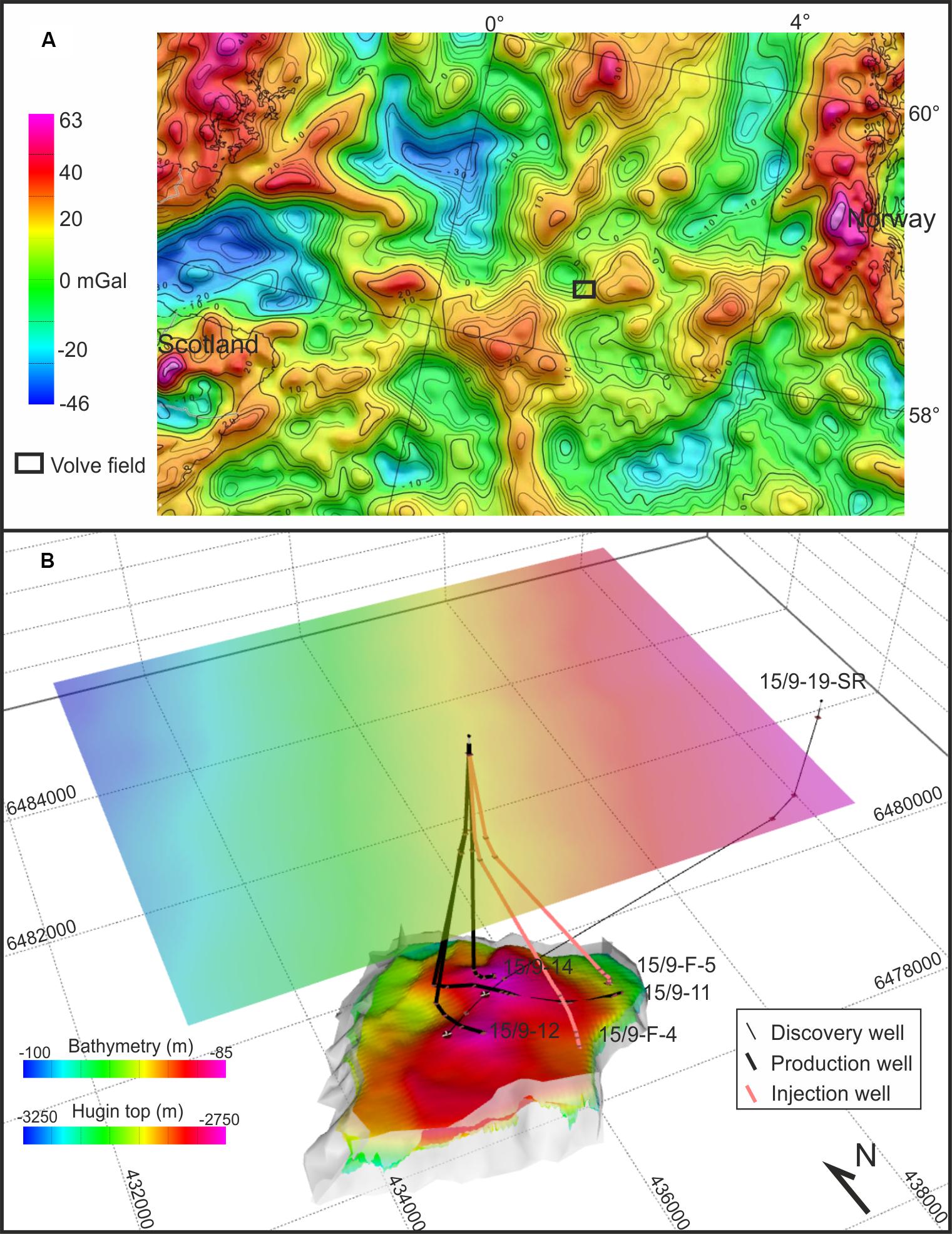
Figure 1. (A) Free-air anomaly at sea and Bouguer anomaly on land over the study region (mod. from Olesen et al., 2010). (B) 3D model of the Volve field reservoir. Light gray surfaces represent bounding faults used to delimit Hugin top and bottom surfaces. Spacing between gray lines in the bounding box provides horizontal and vertical scales: spacing in the X–Y plane is 2 km while spacing in depth is 0.5 km. Coordinates are in ED50 UTM 31N.
After shut down and removal of the production equipment in summer 2017, the entire dataset regarding seismic volumes, well logs, and petrophysical and geological characterization of the field was disclosed by Statoil (now Equinor) in June 20181.
The Volve dataset encompasses over 5 Tbytes of data counting over 11000 files including both raw data and interpretations of the formation tops and faults. It includes also the 3D models used for production simulations as resulting from the seismic data interpretation and well logs. Locations of production and injection wells, daily and monthly reports on production, and injection activities are available as well. Finally, geochemical analyses of formation fluids at reservoir conditions of pressure and temperature are provided together with detailed characterization of the involved formations. The availability for the scientific community of such a detailed and complete database regarding a reservoir system and its production history represents a unique opportunity and allows the community for unprecedented attempts in testing modeling techniques.
Modeling Procedure
In order to provide an input geometry for the forward gravity model, we first created a 3D model of the reservoir using Hugin top and bottom surfaces as provided in the Volve dataset. The surfaces of the main faults in the area were depth-converted as they are provided as two-way travel-times (TWT) in the dataset only. This step was carried out using TWT-depth data provided in well logs and reports on well activities included in the dataset. Finally, the 3D model of the reservoir was obtained by intersection of the top and bottom of the Hugin formation with the bounding faults (Figure 1B). We chose to not include other structures in the model to keep the geometry as simple as possible; moreover, we assume that all bounding faults are sealing – i.e., all density changes are contained within the reservoir volume.
Once the geometry of the reservoir was defined, we discretized the ∼4.3 × 10⁹ m3 Hugin volume in 275642 cubic cells with size 25 m × 25 m × 25 m and included it in a larger 3D mesh with same cell size. In this geometric model, the only surface included together with the Hugin volume is the sea bottom representing the major density contrast between sea water and the underlying rock volume (Figure 2). Despite the seafloor effect is obviously removed by the 4D approach, it was included in the single 3D models to evaluate the gravity signature related to bathymetry. Seafloor is found between 85 and 100 m below sea level, and the bathymetry shows a main step (∼10 m) in the eastern area of the modeled region and a gentle westward descending gradient across the entire area (Figure 1B).
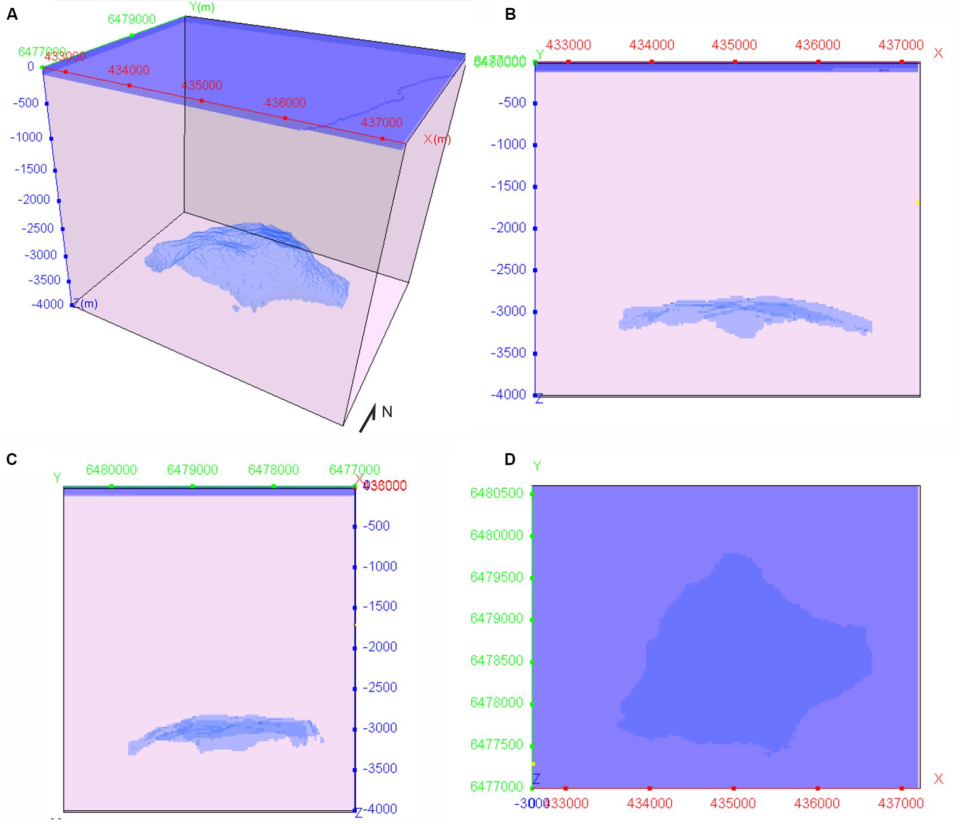
Figure 2. Geometries of the Hugin reservoir and sea water (blue volumes) within the entire model. (A) Perspective, (B) northward, (C) eastward and (D) downward view of the mesh. All scales are in meters. This mesh was used for the pre- and post-production 3D forward models. Cell size is 25 m × 25 m × 25 m. Y axis locates geographic north. Coordinates are in the same system as in Figure 1.
Within the geometric model, we set density values according to the petrophysical and geochemical data recovered from the reports available in the Volve database. In particular, by averaging the density values provided for the units surrounding Hugin, we set a bulk reference density for the volume of 2670 kg m?3. This value was used to calculate density contrasts of sea water volume (−1640 kg m–3) and the Hugin volume (−70 kg m–3) – i.e., we assume that seawater and Hugin have a density of 1030 and 2600 kg m–3, respectively. The density contrasts were used as input for a pre-production 3D forward model.
The procedure to calculate the forward gravity models of the volumes is based on the algorithm proposed by Li and Oldenburg (1998).
The vertical component of the gravity field produced by the density ρ(x,y,z) is given by:
where V is the anomalous mass volume, r0 = (x0, y0, z0) is a vector locating the observation point, r = (x, y, z) locates the source, and γ is the gravitational constant.
Assuming a constant density contrast within each prismatic cell in a 3D orthogonal mesh, the gravity field at the ith observation location is given by:
where ρj and ΔVj are the density and volume of the jth cell, respectively.
To evaluate density changes induced by fluid production and injection, we recovered data from the activity reports provided in the Volve dataset. The total reported volume balance accounting for 1.5 × 10⁹ Sm3 of volumes produced and 30 × 106 Sm3 of injected water is 1.47 × 10⁹ Sm3 (Sm3 stands for standard cubic meters and is referred to 15°C and 1010 × 102 Pa) including oil, gas, and water production and injection. At reservoir conditions (106°C and 3.28 × 10⁷ Pa), this volume becomes 3.21 × 10⁸ m3. At the same temperature and pressure conditions, the fluids in the reservoir have a density of 710 kg m–3 as reported in the geochemical analyses of samples from the discovery well 15/9-19-SR and included in the Volve dataset. Thus, the mass loss in the reservoir, accounting for production and injection activities and reservoir conditions, is of 2.28 × 10¹¹ kg. Considering that injection of water was contemporaneous to production (wells 15/9-F-4 and 15/9-F-5 were active between April 2008 and September 2016), we assume zero compaction of the Hugin sandstones during this period.
If a homogeneous mass loss across the entire reservoir is assumed, after the production each cell in the discretized Hugin volume should weigh 8.27 × 10⁵ kg less than before production – i.e., the total mass loss divided by the total number of cells. In other words, knowing the volume of each cell (1.56 × 10⁴ m3), the production and injection activities resulted in a reservoir formation density loss of ∼53 kg m–3. We note here that this configuration of the post-production model provides no preferential “paths” for density variations within the reservoir because it is not including constraints regarding injection and production wells’ locations. Finally, the achieved density loss value is used to correct the pre-production density of the Hugin volume and perform a post-production 3D gravity forward model of the total volume that is compared with the pre-production model to evaluate gravity changes related to the production activity.
Results
Figure 3 shows the gravity signatures obtained after 3D forward calculation of the pre-production model (Figure 3a) and of the post-production model (Figure 3b) and the differential signature obtained by removing the forward-calculated gravity of the pre-production gravity from the post-production (Figure 3c). All these maps are produced with regular station spacing of 50 m located on sea surface, but similar results are obtained using a double station spacing of 100 m.
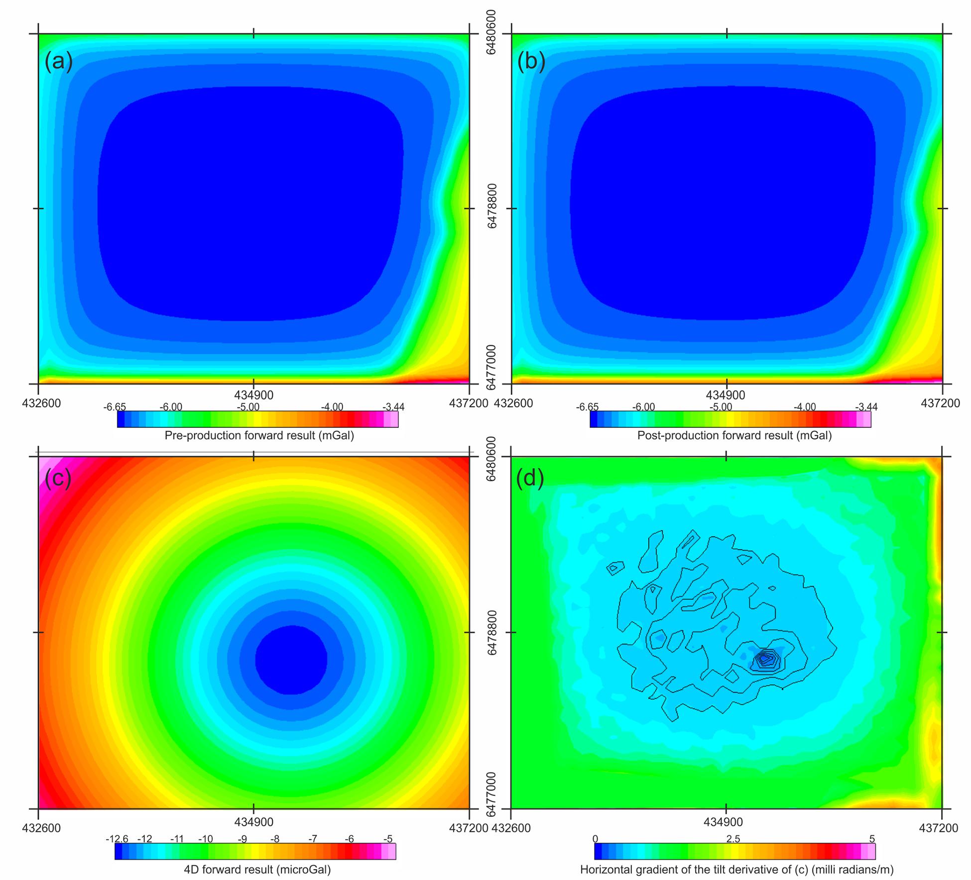
Figure 3. Forward-calculated gravity signature of the pre-production (a) and post-production (b) models. (c) Differential gravity signature calculated by subtraction of pre-production (a) from post-production gravity (b). Spacing between stations for forward calculations is 50 m. (d) Horizontal gradient of the tilt derivative (THDR) computed from (c). Contours locate areas with value <1 milliradians m–1.
Despite the results of the pre- and post-production, forward models are extremely similar in the way that it would not be possible to qualitatively locate any local undulation; the difference between these two gravity data highlights a ∼−13 μGal (−130 × 10–9 m s–2) minimum centered at 435256 E, 6478496 N (ED50, UTM 31N). Considering the modeled volume and the imposed density change, we interpret this minimum as representing the gravity effect of oil, gas, and water production and injection activities at the Volve field between February 2008 and September 2016.
The resulting residuals are in the same order of magnitude than those retrieved in the Sleipner field through gravity data acquisition (e.g., Alnes et al., 2008, 2011).
In a final processing step, we calculate the tilt derivative (Miller and Singh, 1994a; Verduzco et al., 2004) of the anomaly in Figure 3c. The horizontal gradient of the tilt derivative (THDR) is computed in order to locate zero values of the THDR representing the boundary of the causative source (e.g., Miller and Singh, 1994b). Projecting the calculated THDR (Figure 3d) on the reservoir top (Figure 4), we note that the THDR values ≈0 are surrounded by the most producing wells – i.e., 15/9-11, 15/9-12, and 15/9-14 whose production accounts for more than 98% of the total volume (Figure 4B). This evidence supports the former interpretation concerning the gravity minima observed in Figure 3c being caused by reservoir production and injection activities.
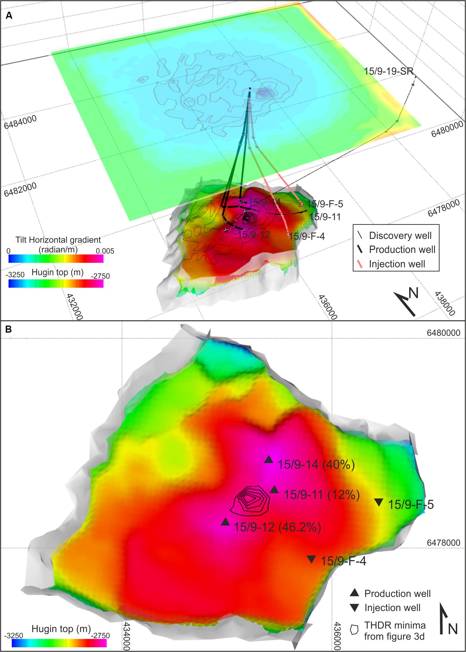
Figure 4. (A) Three-dimensional view of the THDR over the Volve field. The contoured values (thin black lines) were projected to the top Hugin at depth for spatial comparison with reservoir geometry and wells locations. (B) Map view of the reservoir top (i.e., top of the Hugin formation) compared with THDR values <0.6 milliradians m–1 and locations of the contacts between well tracks and top Hugin (triangles). Percentage values within parentheses represent the production over total mass balance achieved by each well. Contour lines are spaced 0.1 milliradians m–1. Horizontal and vertical scales are the same as in Figure 1.
Discussion
The 4D gravity approach is not a new idea to monitor fluid-related density variations, but its application has always relied on high-precision gravity data acquisitions repeated in time and on source depth <2500 m (e.g., Ferguson et al., 2007; Vasilevskiy and Dashevsky, 2007; Alnes et al., 2008, 2011; Elliott and Braun, 2016). In this work, we applied a simple modeling procedure to evaluate the 4D gravity response computed from 3D forward models repeated at pre-production (February 2008) and post-production (September 2016) time steps. This procedure allowed to evaluate the gravity effects of pre-determined density changes in the >2750 m deep Volve reservoir without gravity data acquisition. The procedure was constrained by production data and geometry of the reservoir resulting from seismic and well data.
We assumed sealing conditions of the bounding faults and isotropy of the reservoir volume. Without detailed data about fault behavior and anisotropies within the reservoir levels, we made these assumptions to confine the mass variation within the modeled reservoir and to homogeneously distribute the mass change within the entire reservoir volume. However, the reference volume can be further parametrized in order to locate density changes according to available data or simulated scenarios. For example, to investigate eventual effects on the spatial distribution of density changes after introducing a leaking fault in the model, the reservoir volume should be extended beyond the investigated leaking fault and be parametrized with proper pre-production and post-production density contrasts. Furthermore, volume parametrization allows to model also eventual noise sources – e.g., topography/bathymetry, local density changes in surrounding volumes, as long as these are quantifiable by density or volume changes within the modeled period.
Based on the well-known algorithm proposed by Li and Oldenburg (1998), we modeled the gravity signature without filtering any regional or topographic components that are naturally removed by the differential approach. The only requirements are given by well-constrained geometries of the reservoir, availability of data about produced and injected volumes, and petrophysical properties of the fluids and reservoir formation. All these data are normally produced for oil and gas field characterization.
Interestingly, the procedure locates the causative source of the residual anomaly (Figure 3c), within the area of maximum production, where THDR values ≈ 0 are surrounded by the three most productive wells (Figure 4). In general, it is not surprising that a gravity low is centered over its causative source’s top as we observed in the Volve field (Figure 4). However, what is surprising in this case is the observation per se of a minima being caused by ∼−53 kg m–3 density change at reservoir conditions and whose source is below 2750 m depth. In fact, the Volve field represents a challenging study case for the gravity method because, with a size/depth ratio slightly below the critical value of 1, gravity signatures related to density changes within the modeled volume should not be detectable because of the rapid attenuation of the gravity signal with increasing distance between the observation point and the source – e.g., Stenvold et al. (2008) and references therein.
This outcome strengthens the conclusions obtained by Stenvold et al. (2008) by expanding the retrievable depth for fluid-related density changes below the threshold of 2500 m. Furthermore, the Volve case modeling demonstrates that even without a detailed parametrization of the reservoir units, the simple forward calculation based on reservoir geometry and produced and injected volumes may prove reliable. The applicability of this method depends on the size/depth ratio of the source and on the magnitude of the density change both in terms of the density contrast imposed in the single cell and of thickness of the modeled reservoir carrying a density contrast. Approximating the reservoir shape to a horizontal slice of a cylindrical source (Telford et al., 1990; Stenvold et al., 2008) with radius 1.5 km, the imposed density change of 53 kg m–3 at a depth of 2750 m should produce a 10 μGal gravity change with reservoir thickness of ∼40 m (eq. 1 in Stenvold et al., 2008). Following the same approximation, a reservoir thickness of 100 m with the same density change and the same radius should produce a gravity change of ∼10 μGal at a depth of ∼4000 m. Of course, these approximations are not valid when dealing with complex structures and morphologies such as those often found in real geological contexts like the Volve field.
Considering the position of the gravity minimum and that the post-production input model assumed a homogeneous density change within the entire reservoir volume without constraints regarding injection and production wells, this outcome strengthens the reliability of the retrieved gravity anomaly. Moreover, we expect this approach to retrieve higher amplitude differential gravity residuals when dealing with higher density contrasts than those modeled at the Volve field. In fact, a scenario where reservoir fluids (typically oil, water, and gas) are replaced by CO2 sequestration or gas storage should produce higher density contrasts and in turn should allow to resolve density changes related to gas propagation better.
Conclusion
In this work, we successfully locate the causative source for −53 kg m–3 density changes due to fluid production from a reservoir by 3D forward calculation of gravity at pre- and post-production time steps. The Volve field was chosen as test site because it represents a challenging reservoir with a size/depth ratio slightly below 1, and in these conditions, gravity methods should not allow detection of fluid-induced small density changes. Moreover, the Volve field represents a unique opportunity because in this case, data that usually are kept confidential also after exploitation have been made available to the community allowing the parametrization of the models.
The density change used as input for the post-production model, once removed the pre-production gravity signature, resulted in differential gravity residuals with a −13 μGal minimum above the Volve field. Unsurprisingly, despite the input density variation was distributed within the entire reservoir volume, THDR minimum located on top of the reservoir, between the three most productive wells in the field, whose total production accounted for more than 98% of total mass balance.
This work demonstrates that the 4D gravity method, whether it is constrained to gravity data acquisitions or to forward modeling of known geometries and density changes, represents a reliable technique even in challenging cases. Interestingly, the production-related anomalies observed at 2750 m depth in the Volve field should be theoretically retrievable by seafloor gravimeters with 5 μGal accuracy. However, this goal is still difficult to achieve and likely requires significant efforts in terms of number of stations in order to cover small sources like the Volve field.
Finally, relying on the availability of data that are confidential in the case of oil fields or very expensive to produce for research purposes, this approach has intrinsic limitations in the possibility of being tested in more complex geological scenarios. However, the owners of such data should follow the example of Equinor and release data regarding fields that are no longer exploited; this will likely open new ways in understanding geological and geophysical processes.
Data Availability Statement
Publicly available datasets were analyzed in this study. These data can be found here: Volve data village page: https://www.equinor.com/en/how-and-why/digitalisation-in-our-dna/volve-field-data-village-download.html.
Author Contributions
PM conceived the study, produced the models, and wrote the manuscript.
Funding
This work was supported by the Chieti-Pescara University funds to PM.
Conflict of Interest
The authors declare that the research was conducted in the absence of any commercial or financial relationships that could be construed as a potential conflict of interest.
Acknowledgments
The author thanks the Associate Editor and the two reviewers for their critical reading of the manuscript and constructive comments that improved the manuscript. The author warmly thanks Equinor for providing the Volve dataset and Maurizio Fedi for his constructive comments on a preliminary version of this work.
Footnotes
- ^ https://www.equinor.com/en/how-and-why/digitalisation-in-our-dna/volve-field-data-village-download.html
References
Alnes, H., Eiken, O., Nooner, S., Sasagawa, G., Stenvold, T., and Zumberge, M. (2011). Results from sleipner gravity monitoring: updated density and temperature distribution of the CO2 plume. Energy Procedia 4, 5504–5511. doi: 10.1016/j.egypro.2011.02.536
Alnes, H., Eiken, O., and Stenvold, T. (2008). Monitoring gas production and CO2 injection at the Sleipner field using time-lapse gravimetry. Geophysics 73, WA155–WA161. doi: 10.1190/1.2991119
Blakely, R. J. (1996). Potential Theory in Gravity and Magnetic Applications. Cambridge: Cambridge University Press.
Cooper, C., Dodds, K., and McKnight, R. (2009). “Monitoring programs for CO2 storage,” in A Technical Basis for Cabon Dioxide Storage. CO2 Capture Project, ed. C. Cooper (Amsterdam: Elesevier).
Davis, K., Li, Y., and Batzle, M. (2008). Time-lapse gravity monitoring: a systematic 4D approach with applications to aquifer storage and recovery. Geophysics 73, WA61–WA69.
Devriese, S. G., and Oldenburg, D. W. (2014). “Enhanced imaging of SAGD steam changers using broadband electromagnetic surveying,” in Proceedings fo the SEG Denver 2014 Annual Meeting (Tulsa, OK: SEG) 765–769.
Dressel, I., Barckhausen, U., and Heyde, I. (2018). A 3D gravity and magnetic model for the Entenschnabel area (German North Sea). Int. J. Earth Sci. 107, 177–190. doi: 10.1007/s00531-017-1481-x
Eiken, O., Stenvold, T., Zumberge, M., Alnes, H., and Sasagawa, G. (2008). Gravimetric monitoring of gas production from the Troll feld. Geophysics 73, WA149–WA154.
Eiken, O., Zumberge, M. A., and Sasagawa, G. S. (2000). “Gravity monitoring of offshore gas reservoirs,” in Proceedings of the 70th Annual International Meeting, SEG, Expanded Abstracts (Tulsa, OK: SEG) 431–434.
Elliott, E. J., and Braun, A. (2016). Gravity monitoring of 4D fluid migration in SAGD reservoirs – forward modeling. CSEG Rec. 41, 16–21.
Elliott, E. J., and Braun, A. (2017). On the resolvability of steam assisted gravity drainage reservoirs using time-lapse gravity gradiometry. Pure Appl. Geophys. 174, 4119–4136. doi: 10.1007/s00024-017-1636-1635
Fedi, M., Cella, F., D’Antonio, M., Florio, G., Paoletti, V., and Morra, V. (2018). Gravity modeling finds a large magma body in the deep crust below the gulf of Naples, Italy. Sci. Rep. 8:8229. doi: 10.1038/s41598-018-26346-z
Ferguson, J., Klopping, F., Chen, T., Seibert, J., Hare, J., and Brady, J. (2008). The 4D microgravity method for waterflood surveillance: Part III – 4D absolute microgravity surveys at Prudhoe Bay. Alaska. Geophysics 73, WA163–WA171.
Ferguson, J. F., Chen, T., Brady, J. L., Aiken, C. L. V., and Seibert, J. E. (2007). The 4D microgravity method for waterflood surveillance II — gravity measurements for the Prudhoe Bay reservoir, Alaska. Geophysics 72, I33–I43. doi: 10.1190/1.2435473
Gasperikova, E., and Hoversten, G. M. (2008). Gravity monitoring of CO2 movement during sequestration: model studies. Geophysics 73, WA105–WA112. doi: 10.1190/1.2985823
Hare, J. L., Ferguson, J. F., Aiken, C. L. V., and Brady, J. L. (1999). The 4-D microgravity method for waterflood surveillance: a model study for the Prudhoe Bay reservoir, Alaska. Geophysics 64, 78–87. doi: 10.1190/1.1444533
Isaksen, G. H., Patience, R., van Graas, G., and Jenssen, A. I. (2002). Hydrocarbon system analysis in a rift basin with mixed marine and nonmarine source rocks: the south Viking Graben. North Sea. AAPG Bull. 86, 557–591.
Jacob, T., Bayer, R., Chery, J., and Le Moigne, N. (2010). Time-lapse microgravity surveys reveal water storage heterogeneity of a karst aquifer. J. Geophys. Res. 115, 1–18. doi: 10.1029/2009JB006616
Krahenbuhl, R., and Li, Y. (2012). Time-lapse gravity: a numerical demonstration using robust inversion and joint interpretation of 4D surface and borehole data. Geophysics 77, G33–G43.
Krahenbuhl, R. A., Li, Y., and Davis, T. (2011). Understanding the applications and limitations of time-lapse gravity for reservoir monitoring. Lead. Edge 30, 1060–1068. doi: 10.1190/1.3640530
Mancinelli, P., Pauselli, C., Fournier, D., Fedi, M., Minelli, G., and Barchi, M. R. (2020). Three dimensional gravity local inversion across the area struck by the 2016–2017 seismic events in central Italy. J. Geophys. Res. 125:e2019JB018853. doi: 10.1029/2019JB018853
Mancinelli, P., Pauselli, C., Minelli, G., and Federico, C. (2015). Magnetic and gravimetric modeling of the central Adriatic region. J. Geodynamics 89, 60–70. doi: 10.1016/j.jog.2015.06.008
Mancinelli, P., Porreca, M., Pauselli, C., Minelli, G., Barchi, M. R., and Speranza, F. (2019). Gravity and magnetic modeling of central Italy: insights into the depth extent of the seismogenic layer. Geochem. Geophys. Geosyst. 20, 2157–2172. doi: 10.1029/2018GC008002
Ménoret, V., Vermeulen, P., Le Moigne, N., Bonvalot, S., Bouyer, P., Landragin, A., et al. (2018). Gravity measurements below 10-9 g with a transportable absolute quantum gravimeter. Sci. Rep. 8:12300. doi: 10.1038/s41598-018-30608-30601
Miller, H. G., and Singh, V. (1994a). Semiquantitative techniques for the removal of directional trends from potential field data. J. Appl. Geophys. 32, 199–211. doi: 10.1016/0926-9851(94)90021-3
Miller, H. G., and Singh, V. (1994b). Potential field tilt-a new concept for location of potential field sources. J. Appl. Geophys. 32, 213–217. doi: 10.1016/0926-9851(94)90022-1
Olesen, O., Ebbing, J., Gellein, J., Kihle, O., Myklebust, R., Sand, M., et al. (2010). Gravity Anomaly Map, Norway and Adjacent Areas. Scale 1:3 Million. Trondheim: Geological survey of Norway.
Reitz, A., Krahenbuhl, R., and Li, Y. (2015). Feasibility of time-lapse gravity and gravity gradiometry monitoring for steam-assisted gravity drainage reservoirs. Geophysics 80, WA99–WA110. doi: 10.1190/GEO2014-0217.1
Sasagawa, G. S., Crawford, W., Eiken, O., Nooner, S., Stenvold, T., and Zumberge, M. A. (2003). A new sea-floor gravimeter. Geophysics 68, 544–553. doi: 10.1190/1.1567223
Sobh, M., Ebbing, J., Mansi, A. H., and Götze, H.-J. (2019). Inverse and 3D forward gravity modelling for the estimation of the crustal thickness of Egypt. Tectonophysics 752, 52–67. doi: 10.1016/j.tecto.2018.12.002
Stenvold, T., Eiken, O., and Landro, M. (2008). Gravimetric monitoring of gas-reservoir water influx – A combined flow- and gravity-modeling approach. Geophysics 73, WA123–WA131. doi: 10.1190/1.2991104
Telford, W. M., Geldart, L. P., and Sheriff, R. E. (1990). Applied Geophysics, 2nd Edn. Cambridge: Cambridge University Press.
Van Camp, M., de Viron, O., Watlet, A., Meurers, B., Francis, O., and Caudron, C. (2017). Geophysics from terrestrial time-variable gravity measurements. Rev. Geophys. 55, 938–992. doi: 10.1002/2017RG000566
Vasilevskiy, A., and Dashevsky, Y. (2007). “Feasibility study of 4D microgravity method to monitor subsurface water and gas movements,” in Proceedings of the 77th Annual International Meeting, SEG, Expanded Abstracts (Tulsa, OK: SEG) 816–820.
Verduzco, B., Fairhead, J. D., Green, C. M., and MacKenzie, C. (2004). New insights into magnetic derivatives for structural mapping. Lead. Edge 2004, 116–119. doi: 10.1190/1.1651454
Keywords: 4D modeling, gravity forward modeling, production data constraints, deep source, small density contrast
Citation: Mancinelli P (2020) Four Dimensional Gravity Forward Model in a Deep Reservoir. Front. Earth Sci. 8:285. doi: 10.3389/feart.2020.00285
Received: 04 May 2020; Accepted: 19 June 2020;
Published: 09 July 2020.
Edited by:
Andrea Cannata, University of Catania, ItalyReviewed by:
Ingo Heyde, Federal Institute for Geosciences and Natural Resources, GermanyFilippo Greco, Istituto Nazionale di Geofisica e Vulcanologia (INGV), Italy
Copyright © 2020 Mancinelli. This is an open-access article distributed under the terms of the Creative Commons Attribution License (CC BY). The use, distribution or reproduction in other forums is permitted, provided the original author(s) and the copyright owner(s) are credited and that the original publication in this journal is cited, in accordance with accepted academic practice. No use, distribution or reproduction is permitted which does not comply with these terms.
*Correspondence: Paolo Mancinelli, paolo.mancinelli@unich.it