Exact Likelihood Inference for an Exponential Parameter under Generalized Adaptive Progressive Hybrid Censoring


1
HR Strategy Team, Hyundai Motor Company, Seoul 06797, Korea
2
Division of Mathematics and Big Data Science, Daegu University, Gyeongsan 38453, Korea
*
Author to whom correspondence should be addressed.
Symmetry 2020, 12(7), 1149; https://doi.org/10.3390/sym12071149
Submission received: 10 June 2020
/
Revised: 29 June 2020
/
Accepted: 3 July 2020
/
Published: 9 July 2020
(This article belongs to the Section Mathematics)
Abstract
:In this paper, we propose a new type censoring scheme named a generalized adaptive progressive hybrid censoring scheme (GenAdPrHyCS). In this new type censoring scheme, the experiment is assured to stop at a pre-assigned time. This censoring scheme is designed to correct the drawbacks in the AdPrHyCS. Furthermore, we discuss inference for one parameter exponential distribution (ExD) under GenAdPrHyCS. We derive the moment generating function of the maximum likelihood estimator (MLE) of scale parameter of ExD and the resulting lower confidence bound under GenAdPrHyCS.
1. Introduction
There are many situations in reliability and survival analysis in which units are removed or lost (may occur carelessly or unconsciously) from experimentation before observed. This case is called to as censoring, and a type I and II censoring schemes are typical censoring scheme.
However, type I and II censoring schemes cannot be used if the experimenter wants to remove the live experimental unit at a point other than the final end point of the experiment. Removal during experimentation may be desirable when the surviving units in the experiment that are removed early on can be used for other experiment, or when a compromise between termination time of experimentation and the observation of some extreme lifetimes is required. Therefore, the loss of survival units at points other than the end point may not be avoidable, as in the case of loss of contact with experimental units or unexpected breakage of experimental units. In this reasons and motivations, reliability theoreticians and practitioners considered progressive censoring scheme [1].
Progressive censoring scheme (PrCS) proposed by the Reference [2] can be described as follows. If the first failure is observed, the survival units are removed randomly from the test. Furthermore, if the second failure is observed, the survival units are removed randomly from the test. Finally, if the m-th failure is observed, all the survival units () are removed from the test. In this test, the PrCS is pre-assigned. The m ordered time of observed failure is called PrCS data. Furthermore, we denoted by . See References [3,4,5,6]. The joint probability density function (PDF) of PrCS data can be expressed by
where .
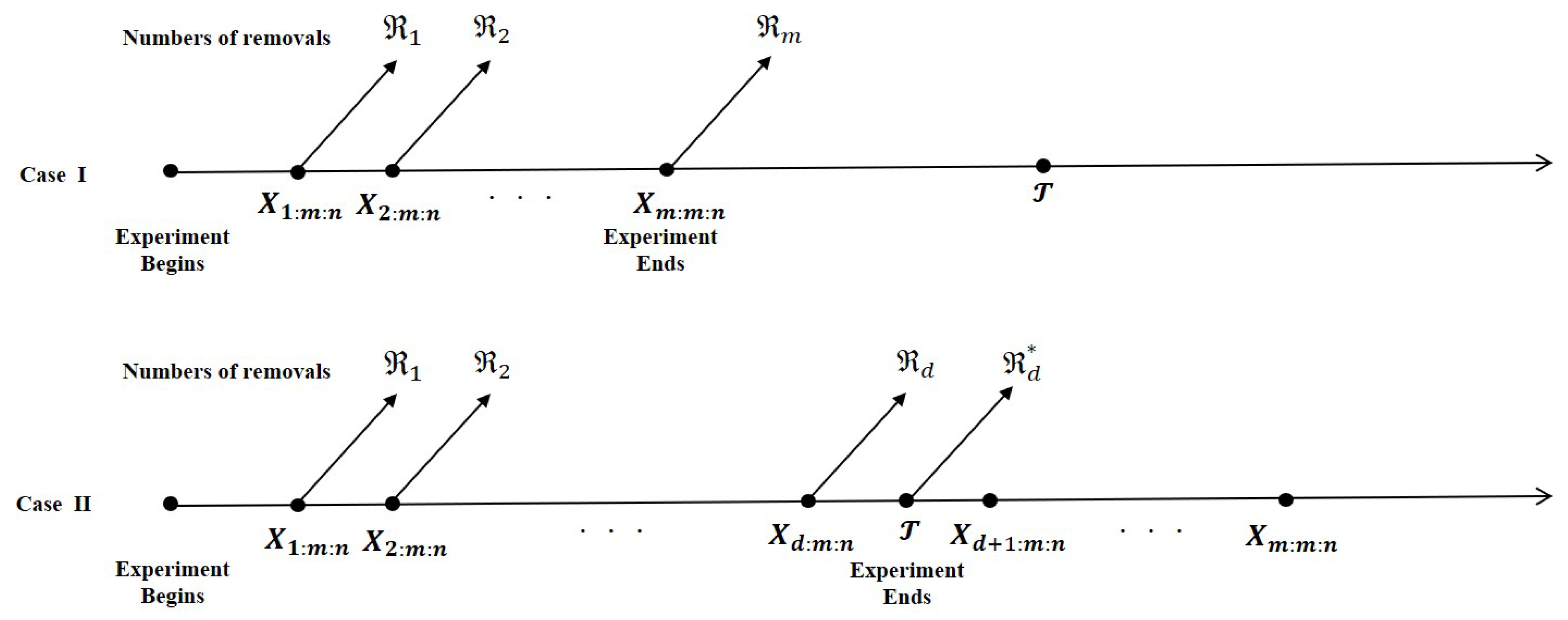
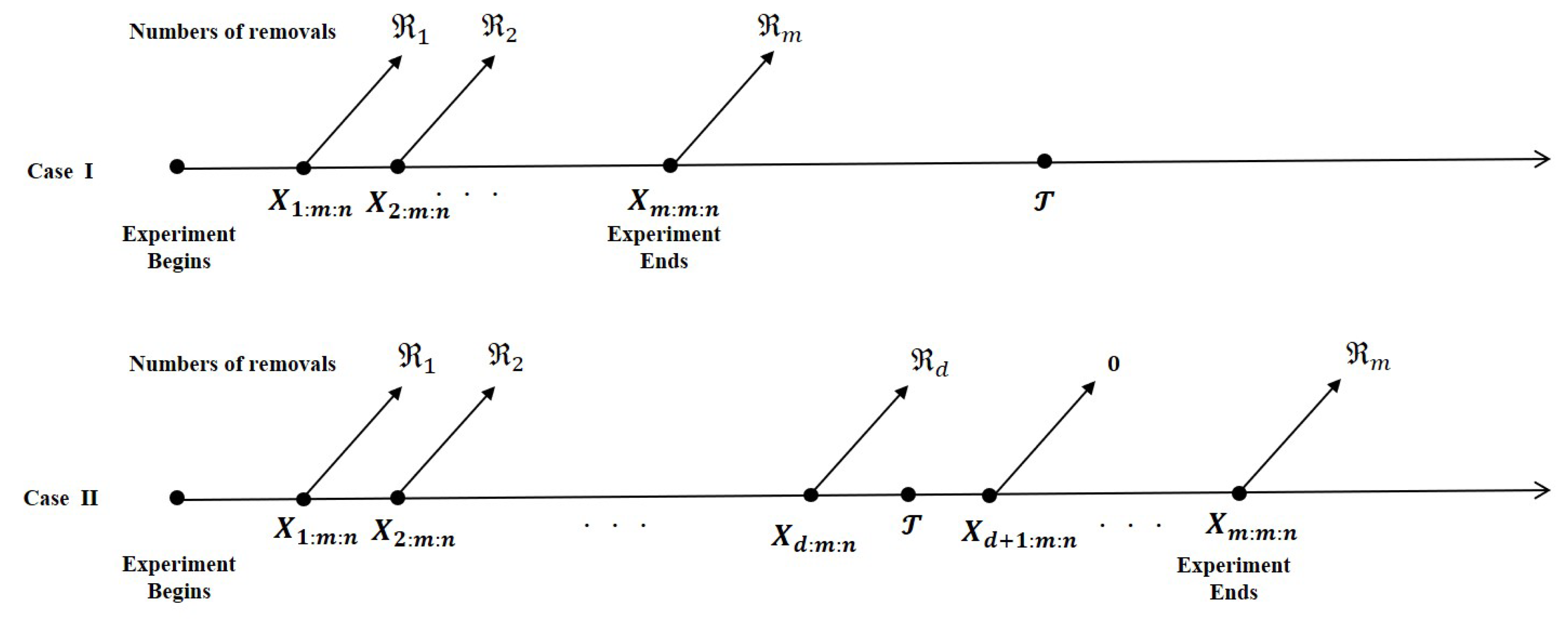
One of the disadvantages of the PrCS is that the time of the experiment can be very long if units are highly reliable. Hence, Reference [7] introduced a progressive hybrid censoring scheme (PrHyCS) in which the reliability test is stopped at a mimimum time of and , where and integer m are pre-assigned. In PrHyCS, the total time required to terminate the experiment does not exceed . Reference [8] derived the exact conditional distribution as well as an interval estimation of the MLE f ExD based on the PrHyCS. A schematic representation of the PrHyCS is presented in Figure 1.
However, the drawback of the PrHyCS is that the number of observed failures is random. Accordingly, it can turn out to be a small number of observed failures (even equal to zero). Therefore, the statistical inference process may not be applicable. Hence, Reference [9] suggest an adaptive progressive hybrid censoring scheme (AdPrHyCS) in which the number of effective sample size m is pre-assigned. In AdPrHyCS, the PrCS is pre-assigned, but the values of some of the may change accordingly during the test. Suppose the experimenter provides a pre-assigned time , which is an ideal total time on test. However, assume that we still allow the experiment to run over time . If the occurs before pre-assigned time , the test stops at the . Otherwise, once the test time passed pre-assigned time but the number of failures has not reached m, we would want to end the test as soon as possible. A schematic representation of the AdPrHyCS is presented in Figure 2.
This setting can be viewed as a design in which we are assured of getting observed failure times for efficiency of statistical inference plus the total time on test will not be too far away from the ideal time . That is to say, after the test passed pre-assigned time , we set and . See References [10,11,12,13,14]. This formulation leads us to end the test as soon as possible if the -th failure time is greater than . Then, there are Cases I and II as follow:
Case I: , if ,
Case II: , if .
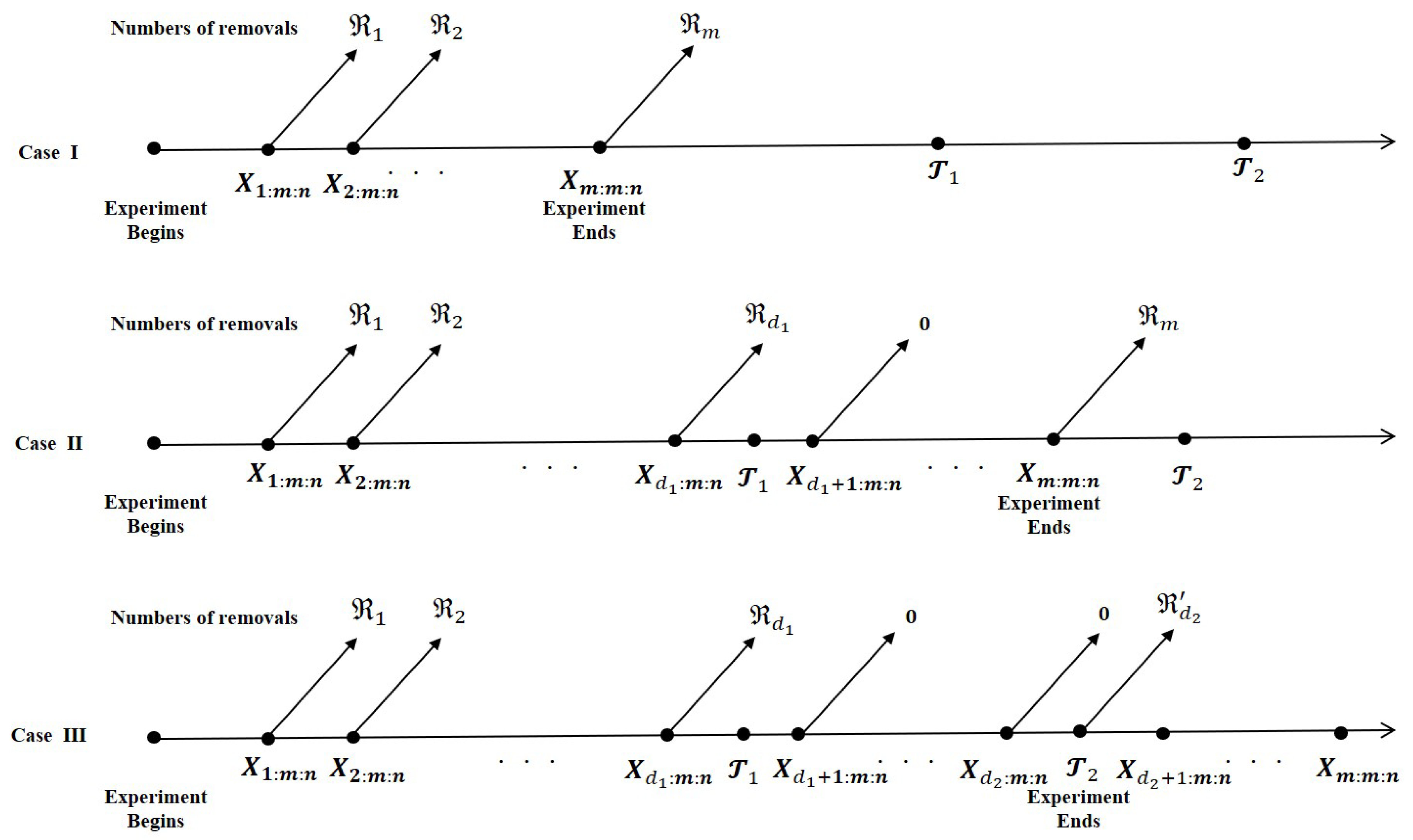
Though the AdPrHyCS assure a pre-assigned number of failures, it has the drawback that it might take a long time to observe a pre-assigned number of failures and terminate the test. In this reason and motivation, we suggest a generalized adaptive progressive hybrid censoring scheme (GenAdPrHyCS) in which the test is assured to end at a pre-assigned time. This censoring scheme is designed to correct the drawbacks in the AdPrHyCS. The survival test based on the GenAdPrHyCS can save both the total time and cost on tests. If the experimenter has prepaid for the use of the facility for units of time, GenAdPrHyCS can be applied. The detailed GenAdPrHyCS description will be described in Section 2.
Furthermore, we will derive the distribution of the MLE of parameter as well as confidence interval for MLE of parameter. In Section 3, we present the results of a numerical study to investigate the MSE, bias, confidence length (CL), and coverage percentages (CP) of the MLE under various GenAdPrHyCS. Furthermore, an illustrative example is presented. Finally, summary and conclusion are presented in Section 4.
2. Model Description and Inference
2.1. Model Description
Consider a life-testing experiment in which n identical units are put on test. GenAdPrHyCS can be explained as follows. The times , , and integer m are pre-assigned such that and , and also pre-assigned PrCS are satisfied . Let and represent the number of failures up to pre-assigned times and , respectively. Likewise, let and be the observed value of and , respectively. When the first failure is observed, the survival units are removed randomly from the test. Furthermore, when the second failure is observed, the survival units are removed randomly from the test and so on. If , terminate the test at (Case I). If , then instead of terminating the test by removing the all survival units at pre-assigned time , continue to observe failures, without any removals, up to time m-th failure (Case II). Therefore, . If , terminate the test at pre-assigned time (Case III). This GenAdPrHyCS modifies the AdPrHyCS by assuring that the test will be terminated by pre-assigned time . Here, the pre-assigned time expresses the longest test time that the experimenter is willing to allow the test to continue. In the GenAdPrHyCS, therefore, there are Cases I, II and III as follow:
Case I: , if .
Case II: , if .
Case III: , if .
Here, , , and are not observed for Case III. A schematic representation of the GenAdPrHyCS is presented in Figure 3.
2.2. MLE
Assume that the observed failure times are independent and identically exponential distribution (ExD) as;
Based on the three scenarios as discussed in the Section 2.1, the likelihood function () can be expressed as;
where . From 2, we obtain the MLE of as
2.3. Exact Inference for MLE
The following Lemma 1 established in Reference [15] is used to derive the explicit expression of the conditional moment generating function (MGF) of MLE.
Lemma 1.
Let where , and let X denote the absolutely continuous random variable with PDF and CDF . Then for , we have
where ; , with the usual conventions that and .
Lemma 2.
- (a)
- The conditional joint density (ConJD) of given , iswhere for .
- (b)
- For and , the ConJD of given and , is
- (c)
- For , the ConJD of given , is
Proof.
Theorem 1.
The MGF of is given by
where , and .
Proof.
The proof of Theorem 1 is given in Appendix A. □
Theorem 2.
With conditional , the conditional PDF of is given by
where , and .
Proof.
The proof of Theorem 2 is given in Appendix B. □
Corollary 1.
Conditional on , the expectation and mean squared error (MSE) of are given by
and
In order to derive a lower confidence bound for , the expression for which is presented in the following theorem is needed.
Theorem 3.
Conditional on , the tail probibility of can be expressed as
where , and .
Proof.
The proof of Theorem 3 is given in Appendix C. □
We shall assume that is an increasing function of . Then, a lower confidence bound for is , where satisfies the equation , and is the observed value of . Similarly, a confidence interval for is , where and satisfy the equations and , respectively.
3. Real Data Analysis and Simulation Results
3.1. Real Data Analysis
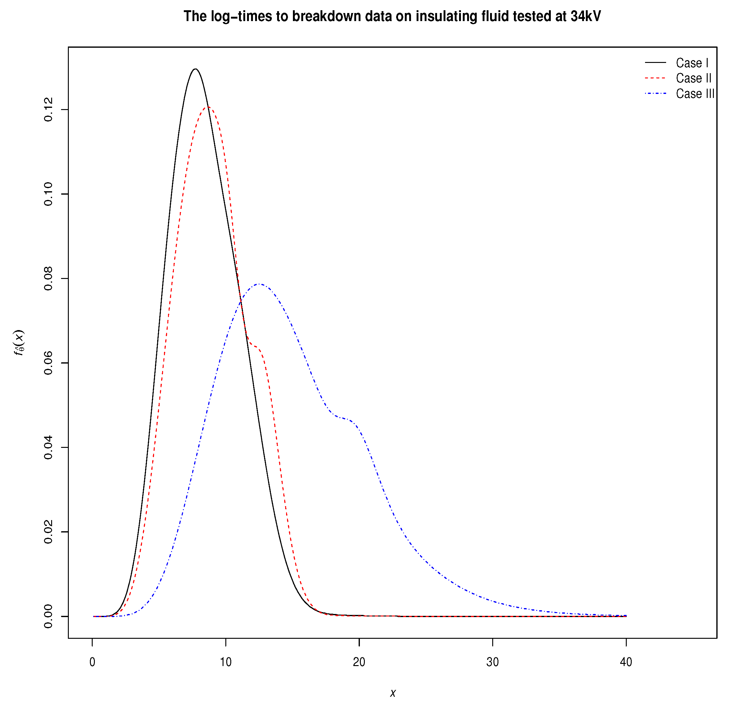
A PrCS data generated from the log-times to breakdown data on insulating fluid tested at 34 kV by Reference [16] is used to illustrate the test statistics discussed earlier. Table 1 represents the PrCS data.
3.2. Simulation Results
We consider various n, m, and . We have used three different PrCS as; Scheme I: and for . Scheme II: and for . Schemes III: and for and m.
For three PrCS, we generate PrCS data. If , we have Case I and the corresponding GenAdPrHyCS data is . If , we have Case II and the corresponding GenAdPrHyCS data is , and . If , we have Case III and we find such that . The corresponding GenAdPrHyCS data is . Without loss of generality, we take in each case. We reiterate the procedure 1000 times in each GenAdPrHyCS. We calculate the average biases of the estimaor, and the corresponding MSEs. The simulation results are presented in Table 3. Furthermore, we calculate the average CL and the corresponding CP. The results are presented in Table 4.
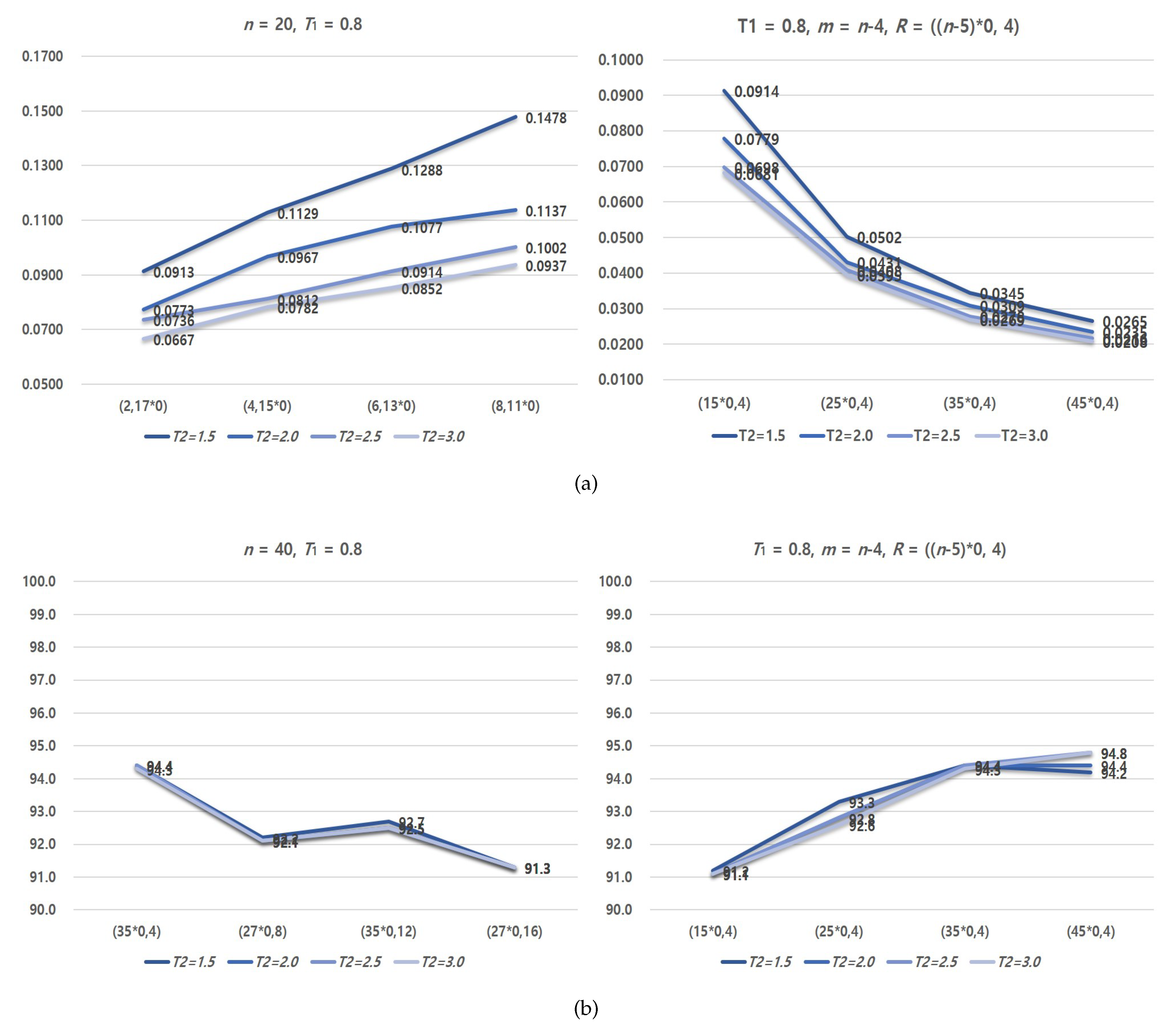
From Table 3 and Figure 5a, the following general observations can be made. The MSEs decrease as sample size n increases. For fixed sample size n, the MSEs decrease generally as the number of PrCS data size m increases. For fixed sample size n and PrCS data size m, the MSEs decreases generally as the time increases. Furthermore, we can observed that the estimaor for PrCS I has smaller MSE and bias than the corresponding estimaor for the other two PrCS.
From Table 4 and Figure 5b, the CL decrease as sample size n increases. For fixed sample size n, the CL decrease generally as the number of PrCS data size m increases. For fixed sample size n and PrCS data size m, the CL decreases generally as the time increases. Furthermore, we can observed that the estimaor for PrCS I has smaller CL than the corresponding estimaor for the other two PrCS. It is observed that the CI works well for all GenAdPrHyCS.
4. Conclusions
There are many situations in reliability and survival analysis in which units are removed or lost (may occur carelessly or unconsciously) from experimentation before observed. This case is called to as censoring, and a type I and II censoring schemes are typical censoring scheme. However, type I and II censoring schemes cannot be used if the experimenter wants to remove the live experimental unit at a point other than the final end point of the experiment. Therefore, the loss of survival units at points other than the end point may not be avoidable. In this reasons and motivations, reliability theoreticians and practitioners considered progressive censoring scheme. One of the disadvantages of the PrCS is that the time of the experiment can be very long if units are highly reliable. Hence, Reference [7] introduced a PrHyCS. Though the AdPrHyCS assure a pre-assigned number of failures, it has the drawback that it might take a long time to observe a pre-assigned number of failures and terminate the test. In this reason and motivation, we suggest a GenAdPrHyCS in which the test is assured to end at a pre-assigned time. This censoring scheme is designed to correct the drawbacks in the AdPrHyCS. The survival test based on the GenAdPrHyCS can save both the total time and cost on tests. Furthermore, we derive the distribution of the MLE of ExD parameter as well as confidence interval for MLE of ExD parameter under GenAdPrHyCS.
Consequently, the MSEs decrease as sample size increases. For fixed sample size, the MSEs decrease generally as the number of PrCS data size increases. For fixed sample size and PrCS data size, the MSEs decrease generally as the time increases. The CL decrease as sample size increases. For fixed sample size, the CL decrease generally as the number of PrCS data size decreases. For fixed sample size and PrCS data size, the CL decrease generally as the time increases. Although we focused on the inference for scale parameter of the ExD, the suggested GenAdPrHyCS can be extended to other distributions.
Author Contributions
Conceptualization, K.L. and H.L.; Software, K.L. and H.L.; Supervision, K.L.; Writing—original draft preparation, K.L. and H.L.; Writing—review and editing, K.L.; Visualization, K.L.; Funding acquisition, K.L. All authors have read and agreed to the published version of the manuscript.
Funding
This work was supported by the National Research Foundation of Korea (NRF) grant funded by the Korea government (MSIT) (NRF-2019R1F1A1043598).
Conflicts of Interest
The authors declare no conflict of interest.
Appendix A. Proof of Theorem 1
Conditional on , the MGF of is given by
For ,
From Lemma 1 with and then factor out of all of the ’s, the above expression can be easily simplified as
For and ,
From Lemma 1 with and then factor out of all of the ’s, the above expression can be easily simplified as
Equation (A3) is obtained by the integration process on the basis of identity that
For ,
From Lemma 1 with and then factor out of all of the ’s, the above expression can be easily simplified as
Appendix B. Proof of Theorem 2
From Theorem 1, the MGF of is given by
Because is the MGF of at , where Y is a gamma random variable with PDF , the theorem readily follows.
Appendix C. Proof of Theorem 3
Let
Then,
References
- Balakrishnan, N.; Aggarwala, R. Progressive Censoring: Theory, Methods and Applications; Birkhauser: Boston, MA, USA, 2000. [Google Scholar]
- Herd, R.G. Estimation of the Parameters of a Population from a Multi-Censored Sample. Ph.D. Thesis, Iowa State College, Ames, IA, USA, 1956. [Google Scholar]
- Górny, J.; Cramer, E. A volume based approach to establish B-spline based expressions for density functions and its application to progressive hybrid censoring. J. Korean Stat. Soc. 2019, 48, 340–355. [Google Scholar]
- Goyal, T.; Rai, P.K.; Maurya, S.K. Bayesian estimation for GDUS exponential distribution under type-I progressive hybrid censoring. Ann. Data Sci. 2020, 7, 307–345. [Google Scholar] [CrossRef]
- Sen, T.; Singh, S.; Tripathi, Y.M. Statistical inference for Lognormal distribution with type-I progressive hybrid censored data. Am. J. Math. Manag. Sci. 2019, 38, 70–95. [Google Scholar] [CrossRef]
- Xie, Y.; Gui, W. Statistical inference of the lifetime performance index with the log-logistic distribution based on progressive first-failure-censored data. Symmetry 2020, 12, 937. [Google Scholar] [CrossRef]
- Kundu, D.; Joarder, A. Analysis of type II progressively hybrid censored data. Comput. Stat. Data Anal. 2006, 50, 2509–2528. [Google Scholar] [CrossRef]
- Childs, A.; Chandrasekar, B.; Balakrishnan, N. Exact likelihood inference for an exponential parameter under progressive hybrid schemes. In Statistical Models and Methods for Biomedical and Technical Systems; Vonta, F., Huber-Carol, C., Limnios, N., Nikulin, M.S., Eds.; Birkhauser: Boston, MA, USA, 2007; pp. 319–330. [Google Scholar]
- Ng, H.K.T.; Kundu, D.; Chan, P.S. Statistical analysis of exponential lifetimes under an adaptive type-II progressively censoring scheme. Nav. Res. Logist. 2010, 56, 687–698. [Google Scholar] [CrossRef] [Green Version]
- Ashour, S.K.; Nassar, M. Inference for Weibull distribution under adaptive type-I progressive hybrid censored competing risks data. Commun. Stat. Theory Methods 2017, 46, 4756–4773. [Google Scholar] [CrossRef]
- Nassar, M.; Abo-Kasem, O.E. Estimation of the inverse Weibull parameters under adaptive type-II progressive hybrid censoring scheme. J. Comput. Appl. Math. 2017, 315, 228–239. [Google Scholar] [CrossRef]
- Sobhi, M.M.A.; Soliman, A.A. Estimation for the exponentiated Weibull model with adaptive type-II progressive censored schemes. Appl. Math. Model. 2016, 40, 1180–1192. [Google Scholar] [CrossRef]
- Xu, B.; Gui, W. Entropy estimation of inverse Weibull distribution under adaptive type-II progressive hybrid censoring schemes. Symmetry 2019, 11, 1463. [Google Scholar]
- Yan, Z.; Wang, N. Statistical analysis based on adaptive progressive hybrid censored sample from alpha power generalized exponential distribution. IEEE Access 2020, 8, 54691–54697. [Google Scholar] [CrossRef]
- Balakrishnan, N.; Childs, A.; Chandrasekar, B. An efficient computational method for moments of order statistics under progressive censoring. Stat. Probab. Lett. 2002, 60, 359–365. [Google Scholar] [CrossRef]
- Viveros, R.; Balakrishnan, N. Interval estimation of parameters of life from progressively censored data. Technometrics 1994, 36, 84–91. [Google Scholar] [CrossRef]
Figure 1.
Schematic representation of PrHyCS.

Figure 2.
Schematic representation of AdPrHyCS.

Figure 3.
Schematic representation of GenAdPrHyCS.

Figure 4.
The PDF of for example.

Figure 5.
The MSE (a) and CP (b) of estimator for some GenAdPrHyCS.


Table 1.
Log-times to breakdown data on insulating fluid tested at 34 kV.
| i | 1 | 2 | 3 | 4 |
| 0.18999 | 0.77997 | 0.95993 | 1.30996 | |
| 0 | 0 | 3 | 0 | |
| i | 5 | 6 | 7 | 8 |
| 2.77986 | 4.84962 | 6.49999 | 7.35000 | |
| 3 | 0 | 0 | 5 |
Table 2.
Inference for .
| C.I for | |||||
|---|---|---|---|---|---|
| Case | MSE | SE. | |||
| Case I | 9.08855 | 14.9261 | 3.6217 | (4.99597, 20.96100) | (5.48302, 18.17892) |
| Case II | 10.80235 | 23.2914 | 4.5846 | (5.98840, 25.00965) | (6.56902, 21.69869) |
| Case III | 11.89555 | 45.7945 | 6.6352 | (9.88020, 41.89090) | (10.85072, 36.28145) |
Table 3.
The MSE and bias of estimator for various GenAdPrHyCS.
| MSE (Bias) | |||||||
|---|---|---|---|---|---|---|---|
| 20 | 0.8 | 18 | (17*0,2) † | 0.0807 (0.0353) | 0.0725 (0.0228) | 0.0650 (0.0154) | 0.0613 (0.0109) |
| (2,17*0) ‡ | 0.0913 (0.0399) | 0.0773 (0.0274) | 0.0736 (0.0200) | 0.0667 (0.0165) | |||
| (1,16*0,1) | 0.0900 (0.4210) | 0.0751 (0.0242) | 0.0669 (0.0176) | 0.0641 (0.0145) | |||
| 16 | (15*0,4) | 0.0914 (0.0286) | 0.0779 (0.0165) | 0.0698 (0.0081) | 0.0681 (0.0070) | ||
| (4,15*0) | 0.1129 (0.0379) | 0.0967 (0.2810) | 0.0812 (0.0198) | 0.0782 (0.0185) | |||
| (2,14*0,2) | 0.1005 (0.0355) | 0.0841 (0.0231) | 0.0774 (0.0168) | 0.0710 (0.0101) | |||
| 14 | (13*0,6) | 0.0863 (0.0188) | 0.0765 (0.0101) | 0.0754 (0.0094) | 0.0752 (0.0094) | ||
| (6,13*0) | 0.1288 (0.0522) | 0.1077 (0.0377) | 0.0914 (0.0267) | 0.0852 (0.0207) | |||
| (3,12*0,3) | 0.1101 (0.0420) | 0.0857 (0.0191) | 0.0790 (0.0123) | 0.0769 (0.0100) | |||
| 12 | (11*0,8) | 0.0856 (0.0133) | 0.0826 (0.0115) | 0.0826 (0.0115) | 0.0826 (0.0115) | ||
| (8,11*0) | 0.1478 (0.0542) | 0.1137 (0.0319) | 0.1002 (0.0270) | 0.0937 (0.0236) | |||
| (4,10*0,4) | 0.1051 (0.0311) | 0.0897 (0.0171) | 0.0839 (0.0121) | 0.0830 (0.0117) | |||
| 30 | 0.8 | 26 | (25*0,4) | 0.0502 (0.0168) | 0.0431 (0.0075) | 0.0408 (0.0023) | 0.0395 (0.0007) |
| (4,55*0) | 0.0613 (0.0256) | 0.0498 (0.0140) | 0.0451 (0.0090) | 0.0426 (0.0059) | |||
| (2,24*0,2) | 0.0551 (0.0223) | 0.0464 (0.0129) | 0.0428 (0.0067) | 0.0408 (0.0030) | |||
| 24 | (23*0,6) | 0.0503 (0.0140) | 0.0446 (0.0050) | 0.0426 (0.0022) | 0.0423 (0.0020) | ||
| (6,23*0) | 0.0658 (0.0247) | 0.0531 (0.0123) | 0.0490 (0.0081) | 0.0463 (0.0061) | |||
| (3,22*0,3) | 0.0553 (0.0194) | 0.0483 (0.0094) | 0.0449 (0.0057) | 0.0429 (0.0029) | |||
| 22 | (21*0,8) | 0.0498 (0.0115) | 0.0444 (0.0040) | 0.0438 (0.0036) | 0.0437 (0.0036) | ||
| (8,21*0) | 0.0682 (0.0326) | 0.0569 (0.0222) | 0.0530 (0.0167) | 0.0488 (0.0116) | |||
| (4,20*0,4) | 0.0554 (0.0245) | 0.0491 (0.0120) | 0.0456 (0.0055) | 0.0442 (0.0039) | |||
| 20 | (19*0,10) | 0.0548 (0.0060) | 0.0512 (0.0036) | 0.0511 (0.0036) | 0.0511 (0.0036) | ||
| (10,19*0) | 0.0824 (0.0344) | 0.0684 (0.0214) | 0.0606 (0.0128) | 0.0572 (0.0108) | |||
| (5,18*0,5) | 0.0649 (0.0205) | 0.0558 (0.0077) | 0.0522 (0.0042) | 0.0513 (0.0037) | |||
| 40 | 0.8 | 36 | (35*0,4) | 0.0345 (0.0124) | 0.0309 (0.0056) | 0.0278 (−0.0007) | 0.0269 (−0.0031) |
| (4,35*0) | 0.0371 (0.0149) | 0.0340 (0.0085) | 0.0317 (0.0057) | 0.0294 (0.0014) | |||
| (2,34*0,2) | 0.0359 (0.0122) | 0.0325 (0.0085) | 0.0295 (0.0025) | 0.0279 (−0.0006) | |||
| 32 | (27*0,8) | 0.0368 (0.0073) | 0.0341 (0.0000) | 0.0323 (−0.0023) | 0.0323 (−0.0023) | ||
| (8,27*0) | 0.0438 (0.0132) | 0.0389 (0.0095) | 0.0360 (0.0051) | 0.0349 (0.0033) | |||
| (4,26*0,4) | 0.0392 (0.0121) | 0.0348 (0.0038) | 0.0343 (0.0007) | 0.0331 (−0.0013) | |||
| 28 | (35*0,12) | 0.0382 (0.0027) | 0.0358 (−0.0002) | 0.0356 (−0.0003) | 0.0356 (−0.0003) | ||
| (12,35*0) | 0.0511 (0.0165) | 0.0436 (0.0099) | 0.0420 (0.0088) | 0.0401 (0.0069) | |||
| (6,34*0,6) | 0.0435 (0.0129) | 0.0388 (0.0042) | 0.0363 (0.0004) | 0.0356 (−0.0003) | |||
| 24 | (27*0,16) | 0.0424 (0.0021) | 0.0423 (0.0020) | 0.0423 (0.0020) | 0.0423 (0.0020) | ||
| (16,27*0) | 0.0650 (0.0247) | 0.0525 (0.0119) | 0.0488 (0.0079) | 0.0462 (0.0059) | |||
| (8,26*0,8) | 0.0485 (0.0102) | 0.0430 (0.0026) | 0.0424 (0.0021) | 0.0423 (0.0020) | |||
| 50 | 0.8 | 46 | (45*0,4) | 0.0265 (0.0070) | 0.0235 (0.0031) | 0.0216 (−0.0010) | 0.0208 (−0.0030) |
| (4,45*0) | 0.0293 (0.0085) | 0.0258 (0.0049) | 0.0236 (0.0011) | 0.0225 (−0.0005) | |||
| (2,44*0,2) | 0.0275 (0.0069) | 0.0243 (0.0040) | 0.0224 (0.0003) | 0.0215 (−0.0015) | |||
| 42 | (41*0,8) | 0.0280 (0.0082) | 0.0256 (0.0017) | 0.0234 (−0.0025) | 0.0234 (−0.0026) | ||
| (8,41*0) | 0.0324 (0.0094) | 0.0288 (0.0042) | 0.0272 (0.0033) | 0.0263 (0.0030) | |||
| (4,40*0,4) | 0.0301 (0.0087) | 0.0265 (0.0043) | 0.0254 (0.0016) | 0.0240 (−0.0015) | |||
| 38 | (37*0,12) | 0.0305 (0.0021) | 0.0275 (−0.0033) | 0.0272 (−0.0035) | 0.0272 (−0.0035) | ||
| (12,37*0) | 0.0410 (0.0144) | 0.0345 (0.0063) | 0.0312 (0.0015) | 0.0296 (0.0004) | |||
| (6,36*0,6) | 0.0340 (0.0089) | 0.0298 (0.0017) | 0.0282 (−0.0023) | 0.0273 (−0.0035) | |||
| 34 | (33*0,16) | 0.0295 (−0.0019) | 0.0286 (−0.0029) | 0.0286 (−0.0029) | 0.0286 (−0.0029) | ||
| (16,33*0) | 0.0396 (0.0048) | 0.0341 (0.0012) | 0.0323 (0.0007) | 0.0311 (0.0000) | |||
| (8,32*0,8) | 0.0326 (0.0036) | 0.0292 (−0.0024) | 0.0287 (−0.0030) | 0.0287 (−0.0030) | |||
| 60 | 0.8 | 54 | (53*0,6) | 0.0217 (0.0041) | 0.0191 (−0.0001) | 0.0180 (−0.0048) | 0.0177 (−0.0058) |
| (6,53*0) | 0.0249 (0.0069) | 0.0210 (0.0013) | 0.0194 (−0.0018) | 0.0188 (−0.0026) | |||
| (3,52*0,3) | 0.0228 (0.0052) | 0.0198 (0.0008) | 0.0187 (−0.0017) | 0.0180 (−0.0051) | |||
| 48 | (47*0,12) | 0.0231 (0.0016) | 0.0213 (−0.0035) | 0.0207 (−0.0044) | 0.0207 (−0.0044) | ||
| (12,47*0) | 0.0296 (0.0088) | 0.0246 (0.0027) | 0.0232 (−0.0011) | 0.0219 (−0.0030) | |||
| (6,46*0,6) | 0.0245 (0.0048) | 0.0225 (−0.0003) | 0.0216 (−0.0026) | 0.0210 (−0.0040) | |||
| 42 | (41*0,18) | 0.0244 (−0.0011) | 0.0234 (−0.0026) | 0.0234 (−0.0026) | 0.0234 (−0.0026) | ||
| (18,41*0) | 0.0323 (0.0094) | 0.0288 (0.0043) | 0.0271 (0.0034) | 0.0263 (0.0030) | |||
| (9,40*0,9) | 0.0276 (0.0077) | 0.0250 (0.0002) | 0.0235 (−0.0025) | 0.0234 (−0.0026) | |||
| 36 | (35*0,24) | 0.0267 (−0.0035) | 0.0267 (−0.0035) | 0.0267 (−0.0035) | 0.0267 (−0.0035) | ||
| (24,35*0) | 0.0368 (0.0145) | 0.0337 (0.0085) | 0.0317 (0.0056) | 0.0295 (0.0013) | |||
| (12,34*0,12) | 0.0297 (0.0020) | 0.0268 (−0.0034) | 0.0267 (−0.0035) | 0.0267 (−0.0035) | |||
† (17*0, 2): (0,0,0,0,0,0,0,0,0,0,0,0,0,0,0,0,0,2); ‡ (2,17*0): (2, 0,0,0,0,0,0,0,0,0,0,0,0,0,0,0,0,0).
Table 4.
The CP and the corresponding CL of estimator for various GenAdPrHyCS.
| Coverage Percentage (Confidence Length) | |||||||
|---|---|---|---|---|---|---|---|
| 20 | 0.8 | 18 | (17*0,2) † | 94.8 (1.0548) | 94.5 (0.9846) | 94.4 (0.9525) | 94.4 (0.9385) |
| (2,17*0) ‡ | 93.8 (1.1183) | 94.0 (1.0371) | 94.3 (0.9945) | 94.4 (0.9709) | |||
| (1,16*0,1) | 94.3 (1.0925) | 94.8 (1.0069) | 94.4 (0.9688) | 94.4 (0.9509) | |||
| 16 | (15*0,4) | 93.2 (1.0608) | 93.1 (1.0083) | 93.1 (0.9894) | 93.1 (0.9869) | ||
| (4,15*0) | 93.8 (1.1865) | 94.0 (1.1043) | 93.5 (1.0559) | 93.2 (1.0340) | |||
| (2,14*0,2) | 93.5 (1.1170) | 93.1 (1.0427) | 93.1 (1.0112) | 93.1 (0.9938) | |||
| 14 | (13*0,6) | 93.5 (1.0837) | 93.4 (1.0595) | 93.3 (1.0577) | 93.3 (1.0575) | ||
| (6,13*0) | 93.5 (1.2875) | 93.1 (1.1916) | 93.4 (1.1359) | 93.4 (1.1056) | |||
| (3,12*0,3) | 93.5 (1.1650) | 93.5 (1.0862) | 93.5 (1.0647) | 93.3 (1.0591) | |||
| 12 | (11*0,8) | 93.8 (1.1490) | 93.8 (1.1446) | 93.8 (1.1446) | 93.8 (1.1446) | ||
| (8,11*0) | 93.8 (1.3988) | 94.2 (1.2792) | 94.0 (1.2301) | 94.0 (1.2006) | |||
| (4,10*0,4) | 93.8 (1.2077) | 93.8 (1.1580) | 93.8 (1.1460) | 93.8 (1.4490) | |||
| 30 | 0.8 | 26 | (25*0,4) | 94.3 (0.8377) | 94.8 (0.7898) | 94.8 (0.7737) | 94.6 (0.7699) |
| (4,55*0) | 94.6 (0.9104) | 94.0 (0.8461) | 94.7 (0.8145) | 94.8 (0.7965) | |||
| (2,24*0,2) | 93.9 (0.8728) | 94.0 (0.8157) | 93.8 (0.7879) | 93.8 (0.7757) | |||
| 24 | (23*0,6) | 93.6 (0.8418) | 93.4 (0.8086) | 93.5 (0.8023) | 93.3 (0.8018) | ||
| (6,23*0) | 94.1 (0.9456) | 94.1 (0.8784) | 94.1 (0.8470) | 93.8 (0.8295) | |||
| (3,22*0,3) | 94.1 (0.8855) | 93.6 (0.8313) | 93.4 (0.8116) | 93.4 (0.8038) | |||
| 22 | (21*0,8) | 93.4 (0.8574) | 93.3 (0.8398) | 93.2 (0.8388) | 93.2 (0.8387) | ||
| (8,21*0) | 93.8 (0.9978) | 93.1 (0.9292) | 93.9 (0.8936) | 94.4 (0.8713) | |||
| (4,20*0,4) | 93.4 (0.9100) | 93.5 (0.8589) | 93.3 (0.8425) | 93.3 (0.8394) | |||
| 20 | (19*0,10) | 93.9 (0.8855) | 93.9 (0.8799) | 93.9 (0.8797) | 93.9 (0.8797) | ||
| (10,19*0) | 93.4 (1.0503) | 93.2 (0.9745) | 93.1 (0.9331) | 93.0 (0.9138) | |||
| (5,18*0,5) | 93.0 (0.9320) | 93.8 (0.8898) | 93.9 (0.8811) | 93.9 (0.8799) | |||
| 40 | 0.8 | 36 | (35*0,4) | 94.4 (0.7193) | 94.4 (0.6765) | 94.4 (0.6573) | 94.3 (0.6520) |
| (4,35*0) | 94.5 (0.7607) | 94.3 (0.7134) | 94.5 (0.6890) | 94.1 (0.6726) | |||
| (2,34*0,2) | 94.3 (0.7376) | 94.2 (0.6947) | 94.3 (0.6694) | 94.3 (0.6580) | |||
| 32 | (27*0,8) | 94.2 (0.7208) | 94.1 (0.6956) | 94.1 (0.6914) | 94.1 (0.6914) | ||
| (8,27*0) | 94.7 (0.8049) | 94.5 (0.7580) | 94.3 (0.7305) | 94.6 (0.7158) | |||
| (4,26*0,4) | 94.5 (0.7583) | 94.4 (0.7134) | 94.1 (0.6979) | 94.9 (0.6929) | |||
| 28 | (35*0,12) | 94.7 (0.7466) | 94.5 (0.7408) | 94.5 (0.7406) | 94.5 (0.7406) | ||
| (12,35*0) | 94.0 (0.8650) | 94.6 (0.8108) | 94.9 (0.7851) | 94.5 (0.7688) | |||
| (6,34*0,6) | 94.7 (0.7854) | 94.7 (0.7501) | 94.5 (0.7418) | 94.5 (0.7406) | |||
| 24 | (27*0,16) | 93.3 (0.8020) | 93.3 (0.8017) | 93.3 (0.8017) | 93.3 (0.8017) | ||
| (16,27*0) | 93.1 (0.9444) | 93.1 (0.8773) | 93.1 (0.8464) | 93.8 (0.8291) | |||
| (8,26*0,8) | 93.6 (0.8227) | 93.4 (0.8031) | 93.3 (0.8019) | 93.3 (0.8017) | |||
| 50 | 0.8 | 46 | (45*0,4) | 94.2 (0.6377) | 94.4 (0.6011) | 94.8 (0.5834) | 94.8 (0.5773) |
| (4,45*0) | 94.0 (0.6664) | 94.5 (0.6278) | 94.5 (0.6056) | 94.5 (0.5937) | |||
| (2,44*0,2) | 94.9 (0.6507) | 95.0 (0.6137) | 94.7 (0.5927) | 94.7 (0.5827) | |||
| 42 | (41*0,8) | 94.8 (0.6403) | 94.8 (0.6107) | 94.7 (0.6035) | 94.8 (0.6033) | ||
| (8,41*0) | 94.5 (0.6984) | 94.1 (0.6565) | 94.9 (0.6360) | 94.1 (0.6245) | |||
| (4,40*0,4) | 94.8 (0.6668) | 94.8 (0.6284) | 94.9 (0.6117) | 94.8 (0.6050) | |||
| 38 | (37*0,12) | 94.6 (0.6461) | 94.8 (0.6340) | 94.8 (0.6337) | 94.8 (0.6337) | ||
| (12,37*0) | 94.9 (0.7398) | 94.9 (0.6919) | 94.5 (0.6666) | 94.4 (0.6541) | |||
| (6,36*0,6) | 94.8 (0.6824) | 94.7 (0.6462) | 94.6 (0.6356) | 94.8 (0.6337) | |||
| 34 | (33*0,16) | 94.7 (0.6719) | 94.7 (0.6703) | 94.7 (0.6703) | 94.7 (0.6703) | ||
| (16,33*0) | 94.4 (0.7715) | 94.3 (0.7272) | 94.6 (0.7050) | 94.2 (0.6920) | |||
| (8,32*0,8) | 94.7 (0.6880) | 94.7 (0.6712) | 94.7 (0.6702) | 94.7 (0.6702) | |||
| 60 | 0.8 | 54 | (53*0,6) | 94.8 (0.5796) | 94.9 (0.5469) | 94.3 (0.5332) | 94.2 (0.5306) |
| (6,53*0) | 94.4 (0.6136) | 94.9 (0.5763) | 94.9 (0.5567) | 94.5 (0.5465) | |||
| (3,52*0,3) | 95.2 (0.5956) | 95.2 (0.5606) | 94.9 (0.5429) | 94.2 (0.5337) | |||
| 48 | (47*0,12) | 94.1 (0.5814) | 94.2 (0.5646) | 94.2 (0.5633) | 94.2 (0.5633) | ||
| (12,47*0) | 94.5 (0.6523) | 94.1 (0.6123) | 94.9 (0.5909) | 94.5 (0.5792) | |||
| (6,46*0,6) | 94.3 (0.6114) | 94.0 (0.5776) | 94.1 (0.5664) | 94.2 (0.5637) | |||
| 42 | (41*0,18) | 94.9 (0.6055) | 94.8 (0.6033) | 94.8 (0.6033) | 94.8 (0.6033) | ||
| (18,41*0) | 94.5 (0.6981) | 94.1 (0.6564) | 94.9 (0.6359) | 94.1 (0.6244) | |||
| (9,40*0,9) | 94.7 (0.6343) | 94.9 (0.6078) | 94.8 (0.6034) | 94.8 (0.6033) | |||
| 36 | (35*0,24) | 94.3 (0.6510) | 94.3 (0.6510) | 94.3 (0.6510) | 94.3 (0.6510) | ||
| (24,35*0) | 94.5 (0.7592) | 94.3 (0.7129) | 94.4 (0.6886) | 94.0 (0.6725) | |||
| (12,34*0,12) | 94.3 (0.6621) | 94.3 (0.6513) | 94.3 (0.6510) | 94.3 (0.6510) | |||
† (17*0, 2): (0,0,0,0,0,0,0,0,0,0,0,0,0,0,0,0,0,2); ‡ (2,17*0): (2, 0,0,0,0,0,0,0,0,0,0,0,0,0,0,0,0,0).
© 2020 by the authors. Licensee MDPI, Basel, Switzerland. This article is an open access article distributed under the terms and conditions of the Creative Commons Attribution (CC BY) license (http://creativecommons.org/licenses/by/4.0/).
Share and Cite
MDPI and ACS Style
Lee, H.; Lee, K. Exact Likelihood Inference for an Exponential Parameter under Generalized Adaptive Progressive Hybrid Censoring. Symmetry 2020, 12, 1149. https://doi.org/10.3390/sym12071149
AMA Style
Lee H, Lee K. Exact Likelihood Inference for an Exponential Parameter under Generalized Adaptive Progressive Hybrid Censoring. Symmetry. 2020; 12(7):1149. https://doi.org/10.3390/sym12071149
Chicago/Turabian StyleLee, Hyojin, and Kyeongjun Lee. 2020. "Exact Likelihood Inference for an Exponential Parameter under Generalized Adaptive Progressive Hybrid Censoring" Symmetry 12, no. 7: 1149. https://doi.org/10.3390/sym12071149
Note that from the first issue of 2016, this journal uses article numbers instead of page numbers. See further details here.