Evaluation of Traffic Assignment Models through Simulation


Department of Civil Engineering, University of Burgos, 09001 Burgos, Spain
Sustainability 2020, 12(14), 5536; https://doi.org/10.3390/su12145536
Submission received: 15 June 2020
/
Revised: 2 July 2020
/
Accepted: 7 July 2020
/
Published: 9 July 2020
(This article belongs to the Special Issue Traffic Flow Modelling and Simulation towards Sustainable Transportation)
Abstract
:Assignment methodologies attempt to determine the traffic flow over each network arc based on its characteristics and the total flow over the entire area. There are several methodologies—some fast and others that are more complex and require more time to complete the calculation. In this study, we evaluated different assignment methodologies using a computer simulation and tested the results in a specific case study. The results showed that the “all-or-nothing” methods and the incremental assignment methods generally yield results with an unacceptable level of error unless the traffic is divided into four or more equal parts. The method of successive averages (MSA) was valid starting from a relatively low number of iterations, while the user equilibrium methodologies (approximated using the Frank and Wolfe algorithm) were valid starting from an even lower number of iterations. These results may be useful to researchers in the field of computer simulation and planners who apply these methodologies in similar cases.
1. Introduction
Traffic assignment techniques can be used to assess traffic intensities on a track or road system based on its physical and functional characteristics and the potential traffic that can use it.
An assignment process has two stages. First, it is necessary to determine the possible traffic that can be used by the network, which is usually expressed through current and future origin/destination matrices. Based on this data, in the second stage of the process, this potential traffic is assigned to each of the sections of a given road network. There are a multitude of procedures for this purpose, most of which are empirical and based on statistical observations of user behavior, certain track conditions, and the traffic itself. Procedures with a higher level of precision are, of course, more complicated. However, we cannot forget that we are starting from an estimate of future potential traffic; therefore, each result must be studied by a decision-maker in order to develop appropriate contrasts and produce final results that are consistent with the analyzed situation.
There are several assignment methodologies, some of which have already been compared in certain case studies, although usually not all at once, and only sometimes using simulation techniques [1,2]. The assignment stage has been analyzed at times as an intermediate problem between optimization and equilibrium issues [3]. We can also attempt to analyze the zonal distribution and assignment stages together, as was performed by Tan et al. [4] in a study in which the use of Intelligent Transport Systems (ITS) was incorporated. The number of possible applications of assignment methodologies is enormous, among which we can include their adaptation to multimodal networks as especially novel [5], their use to minimize the environmental impact of traffic [6] and the damage caused to infrastructure by traffic [7], or to optimize the process of searching for a place to park a vehicle [8]. In addition, if we add the use of simulation with computer tools to this [9,10], the number of possibilities is greatly increased.
However, the assignment problem is not only associated with road traffic, but also with other means of transport. For example, within road networks, assignment methods are applied to private vehicles, including taxis and autonomous vehicles and public transportation (PT). For example, Long et al. [11] introduced the concept of the expected rate of return of taxi drivers and performed a dynamic taxi traffic assignment problem supposing real-time traffic information provision; Bischoffa and Maciejewski [12] analyzed the possible effect of a city-wide replacement of private cars with autonomous taxi fleets; Heilig et al. [13] used a microscopic travel demand model to simulate the mode choice behavior in the assumption of the existence of a large autonomous mobility on demand service instead of private cars; and Poulhès and Berrada [14,15] analyzed the effect of dial-a-ride services on the assignment problem. Within the PT assignment problem, Liu and Ceder [16] and Eltved et al. [17] considered different schemes for that; Cats and Hartl [18] focused on the discomfort that causes congestion on PT users and how it affects their choices; and Nuzzolo and Comi [19] included big data issues to this modeling.
With railway transport, there are also interesting studies that employ these techniques to estimate the passenger load on each route. Thus, Lin et al. [20] investigated the railway passenger pricing problem, supposing that operators could modify ticket prices to optimize the system’s performance; Xu et al. [21] proposed a dynamic assignment problem for urban rail transit networks considering queuing process, capacity constraints, and congestion effects; and Gao and Wu [22] proposed a method to calculate the proportion of passengers on each path based on the entry and exit time records of users.
In the maritime domain, assignment methods are also applicable and there are several studies that have analyzed the assignment problem by considering traffic assignment close to seaports. Venturini et al. [23] and Iris et al. [24] studied the integrated berth allocation in seaport container terminals; Li and Jia [25] modeled the traffic scheduling problem as a mixed integer linear program to minimize the berthing and departure delays of vessels; Han et al. [26] studied a storage yard management problem if the loading and unloading activities are both heavy and concentrated; and Iris et al. [27] formulated a mathematical model for the containership loading problem, where the terminal has the right to decide which specific container to load for each slot.
In air transportation, we can find some examples of the application of assignment methods. For instance, Ganić et al. [28] and Ho-Huu et al. [29] developed mathematical models of air traffic assignment in order to minimize the noise effects on population, and Starita et al. [30] considered future capacity provision in terms of the available man-hours of air traffic controllers.
Finally, several studies have considered two or more means of transport simultaneously in a multimodal scenario. Thus, Yu and Guo [31] developed a tri-level combined-mode traffic assignment model; Pi et al. [32] included heterogeneous traffic on roads, parking availability, and travel modes (such as solo-driving, carpooling, ride-hailing, public transit, and park-and-ride); Macedo et al. [33] proposed an efficient traffic assignment, where users are not only concerned about travel times, but also about global and local pollutant emissions; Jiang et al. [34] included the car–truck interaction paradox in assignment problems; and Dimitrov et al. [35] modeled the interaction between buses, passengers, and cars on a bus route.
Some researchers have applied these methodologies in a specific case study, often with the support of computer simulation [36,37,38,39], while others have attempted to assess different techniques or even propose novel ones [40,41,42,43,44,45]. Among the first ones, Zhang et al. [36] integrated an activity-based travel demand model with a dynamic traffic assignment model for the Baltimore Metropolitan Council; Shafiei et al. [37] developed a simulation-based dynamic traffic assignment model of Melbourne, Australia; Zhu et al. [38] used dynamic traffic assignment for a case study in Maryland; and Kucharski and Gentile [39] applied the Information Comply Model on different situations, including a corridor in the North of Kraków, Poland, and the Sioux-Falls network. Within the latter ones, Zhang et al. [40] analyzed the calibration of dynamic traffic assignment models applying the extended Kalman filter; Prakash et al. [41] presented a dimensionality reduction of the assignment model’s calibration problem based on principal components; Du et al. [42] focused on the dynamic traffic assignment problem on large-scale expressway networks, especially under the condition of traffic events (such as severe weather, large traffic accidents, etc.) and proposed an approximate solution algorithm; Lin and Chen [43] developed a simulation-based multiclass, multimodal traffic assignment model for evaluating the traffic control plans of planned special events; Batista and Leclercq [44] studied a regional dynamic traffic assignment framework for a macroscopic fundamental diagram considering stochasticity on both the trip lengths and the regional mean speed; and Bagdasar et al. [45] examined discrete and continuous optimization and equilibrium-type problems and made a comparison of them with the Beckmann cost function.
Finally, we can cite some interesting studies that consider multi-class, multi-modal, and elastic demand traffic for assignment models. Cascetta [46] covered all the issues on traffic assignment; Cantarella [47] provided a highlight on traffic assignment with elastic demand; and Cantarella et al. [48,49,50] proposed an overview of solution algorithms for traffic assignment, presenting a general fixed-point formulation for the multi-user stochastic equilibrium assignment with variable and elastic demand and comparing it with other approaches.
Following this line of research, the main objectives of this study are: (1) to develop an assignment model for a specific case study (the new B-40 highway in Barcelona, Spain) and implement it using traffic macro-simulation tools; and (2) to evaluate the influence of the use of different assignment models on the results and the numbers of iterations in them.
This paper is structured as follows. After a brief introduction, Section 2 outlines the main techniques used in the modeling work performed in this study. Section 3 contains a description of the case study and the principles adopted for delimitation, zonification, and obtaining the base origin/destination matrix. The principles adopted for applying the general methodologies to the specific case study that is being analyzed are then set out in Section 4. Section 5 contains an evaluation of the best assignment methodology for the specific case study to be analyzed. Finally, in Section 6, we discuss our results and the main conclusions drawn from the full study.
2. Methods for Traffic Assignment
Potential users of a transportation system in which there are different alternative itineraries generally have incomplete information about the conditions of each section; however, they must make their decision with these inaccurate data. These data include the length of each segment, the quality of the track (in terms of layout, pavement, and safety conditions), and, finally, the degree of congestion at all times, which decisively affects the vehicle’s speed and, therefore, the time spent on the route. The possibility of knowing the above data ranges from high to low. In addition, with regard to congestion, the knowledge that each driver has is very subjective and is generally based on his/her previous experiences, since in very few cases does he/she have information about the actual situation.
Typically, when choosing from several possible itineraries, we consider different types of factors (e.g., distance, travel time and/or cost, comfort, and toll, if any) that are usually grouped into a single variable called generalized cost. In practice, the process that we need to follow in order to assign traffic to the existing road network in a given area of study has the following steps:
- Zone division. First, the entire study area to be analyzed must be divided into zones of more or less homogeneous characteristics.
- Origin/destination matrix construction. Once the study area has been divided into zones, we need to construct a matrix that lists the movements of each origin/destination pair. We should also distinguish between light and heavy vehicles, since the conditions for the assignment of each type of vehicle are different.
- Definition of road networks. Each defined zone is represented by its centroid, which is the fictional place that generates or attracts all trips in the area. All zones must be joined to one another through the existing transportation system and, if applicable, through the future one (constituting two separate transport networks: a current one and a future one).
- Calculation of travel costs and/or times. For each of the sections of the considered network (current and future), the generalized cost of travelling along it under certain traffic conditions must be determined. It is desirable to calculate the costs for various traffic levels in order to take into account the capacity of each segment, or even do it dynamically at each iteration of the process, depending on the traffic supported by each part of the network.
- Assignment. Using the origin and destination data, it is advisable to calculate the traffic intensities for the existing network in the current situation, and then compare the results obtained with the traffic accounts that have been made. Once this check has been carried out, each of the movements in the origin/destination matrix is assigned to the current and future networks. A separate assignment should be performed for light and heavy vehicles and for various driving conditions. The application of computer tools to traffic assignment models has resulted in the creation of new methods that introduce a greater number of theoretical complications but are perfectly applicable nowadays.
Among the wide variety of methods for traffic assignment (or methods for calculating the traffic load on the network), we used the following, which are those that are used in practice in most cases [51]:
- all-or-nothing assignment
- stochastic assignment
- simulation methodologies
- proportion-based methodologies
- assignment with congestion
- wardrop equilibrium
- speed adaptation
- incremental assignment
- the successive averages method
2.1. All-or-Nothing Assignment
This is the simplest of all assignment methods and results from the load of all journeys to the minimum cost path between the nodes. The costs are initially fixed for all segments in the network: i.e., the speed/flow ratio function is not considered.
While it is simple, it has significant drawbacks. It is an unstable method because small changes in the travel time of a segment can drastically change which routes are chosen to form the minimum cost path. This method ignores limits on the capacity of each segment and the number of times that they have been used in the assignment, so the result may result in little relation to the real flow in the network. In addition, it does not allow for variations between users. For these reasons, if in a study we include a new alternative route and use this methodology, we usually find that all trips head for the new path (the so-called “vacuuming effect”), when, in reality, there will be a distribution of travel through the segments of the network.
A number of modifications have been made to this “base” methodology, such as the one by Lee and Oduor [52], which includes parameters from a GIS (Geographic Information System) network that improve the model’s results.
2.2. Stochastic Assignment
Stochastic assignment distributes the trips of each O/D (Origin/Destination) pair between different paths of the multiple alternatives that connect them. We can sort these methodologies into two kinds: those based on simulation and those based on proportions.
In simulation-based methodologies, which often use the Monte Carlo simulation [53] to represent the variability among users in terms of their perception of network costs, the following assumptions are often made:
- For each segment, it is necessary to differentiate the objective costs, which are measured or estimated by an observer (modeler), from the subjective costs, which are perceived by each user. It is accepted that the target cost roughly matches the average of the subjective costs, which are randomly distributed according to a given probability function. By analyzing the literature on this topic, we can find different assumptions regarding the distribution of these subjective costs. For example, Burrel [53] adopts a uniform distribution, while other authors adopt a normal distribution.
- The distributions of costs perceived by users are independent.
- Users choose the route that minimizes their perceived travel cost: i.e., the sum of the costs of each used section.
Although these methods are simple and relatively quick to apply, they have certain drawbacks. For instance, the assumption that the perceived costs of each section are independent may not be true when users have a certain predisposition to the use of certain types of infrastructure (high-capacity highways, as an example). In addition, the effect of congestion is not explicitly taken into account. However, these methods do allow us to distribute the trips in such a way that the “optimal” paths for the modeler turn out to be the ones with the highest amount of traffic; however, they do not convey the total number of trips. Moreover, it is not necessary to know the flow–speed functions of each section, which makes these methods easier to apply, although sometimes this can be a limitation.
In proportion-based methods, as their name suggests, the fraction of trips assigned to a particular path is equal to the probability of choosing it, which is calculated using a logit-type route choice model. The lower the generalized cost of one path as compared with the others, the greater its chance of being chosen. However, with this methodology, the only alternative paths that have traffic are those that are considered to be “reasonable”—that is, those that separate the user from the origin point and bring them to the destination point. The travel time for each segment in a stochastic assignment is a fixed set of input data and is not dependent on the volume that it supports. Therefore, these methods are not equilibrium methods, nor are they valid in situations of congestion.
According to the single path method [54], the trips between an i–j origin/destination pair along the r-path, Tijr, would result in:
where Tij is the total number of trips from i to j, Cijk is the generalized cost from i to j using the k-path, Ω is a parameter (usually 1), and k is the number of reasonable paths from i to j. Ω can be used to control the distribution of trips between routes; thus, depending on their (always positive) value, cheaper routes tend to concentrate trips, or, on the contrary, distribute them more uniformly among the possible reasonable paths.
2.3. Assignment with Congestion
Regarding congestion-side assignment techniques, the methodologies that researchers most commonly use when requiring an adequate level of detail are equilibrium methods. These methods take into account the dependence between the flow of a section and its generalized travel cost, and calculate both of them simultaneously so that they are consistent. Equilibrium algorithms require the iteration of flow assignments and the recalculation of travel times. Despite the additional computational load, equilibrium methods are almost always preferable to other assignment methods.
The main behavioral assumptions are that each traveler has all of the information about the attributes of network alternatives, all travelers choose routes that minimize their travel time or cost, and all travelers—of the same category—assign the same value to all of the network attributes.
According to the first equilibrium principle, which was proposed by Wardrop [55] and is called “user equilibrium” (UE), no individual traveler can reduce his/her travel time unilaterally by changing his/her path [56]. One consequence of the UE principle is that all of the roads that an O/D pair uses have the same minimum cost, while unused roads have equal or higher costs. Unfortunately, this is not an absolutely realistic description of congested traffic networks, although it can be considered to be sufficiently approximate. The mathematical notation for these expressions is as follows (bearing in mind that, in addition, the conditions of continuity, conservation, and non-negativity of flows must be met):
where cp is the unit cost in the equilibrium state, Pw is the set of paths that connect the pair w, and hp is the flow of path p.
In addition, Wardrop [55] proposed a second alternative to assigning traffic to the network, which takes the name of “system equilibrium.” According to this alternative, under balanced conditions, traffic should be distributed so that the total cost of operation of the network is the minimum possible cost. Computationally, it is similar to the first principle, as expressed in Equation (2), but it replaces unit costs with marginal costs:
where fa and hp are the flows of section a and path p, respectively, CMa and CMp are their respective marginal costs, and ca and cp are their respective unit costs.
In either case (the first principle is most commonly used, since it responds more to the actual “self-interested” behavior of users), we obtain a system of equations, the solution of which would be the flows in sections or on paths.
Another type of model is that of speed adaptation. The simplest of these models, called direct adaptation, is based on all-or-nothing methodologies. However, it differs from them in that, once it assigns traffic, it recalculates the travel times or costs of each section, and then reapplies the all-or-nothing method with the new values. This process can be iterated indefinitely. However, this approach has a major drawback, as the selected paths usually change at each iteration, and the method does not converge to a single solution.
Therefore, in order to try to reduce these oscillations, a methodology was proposed that uses the average of the speeds of two or more all-or-nothing assignments in each iteration. This methodology, called speed-weighted adaptation, is not a real improvement, as it continues to assign all traffic to a single minimum path, which is also usually different in each iteration.
The incremental assignment methodologies are, again, based on the all-or-nothing concept. In this case, however, they introduce a significant improvement by making the results more realistic. In the first step, the demand matrix is split into parts (not necessarily equal ones). The first portion is assigned using the all-or-nothing method and, once the flows are entered, the travel times of each section are recalculated. Then, with the new travel times, the second fraction of the demand matrix is allocated using the all-or-nothing method, and the travel times of each section are recalculated again. This continues until all of the fractions have been assigned. Commonly used values for the fractions are [51]: 0.4, 0.3, 0.2, and 0.1. The end result provides us with flows that are distributed between routes and not assigned in their total to the initially shorter one, which more closely approximates reality.
Theoretically, the larger the number of fractions considered, the more likely it is that trips will be distributed among a greater number of roads. However, even if the demand matrix is divided into very small fractions, this method may never converge to the solution when using the Wardrop balance, as the flow that is already assigned to a section cannot be suppressed or modified. In any case, it is clear that its simplicity and ease of use and the possibility of interpreting its results as the accumulation of congestion during peak periods make it an interesting method.
Finally, the method of successive averages (MSA) is another variant of the all-or-nothing method. In each iteration, the flow of a section is calculated as a linear combination of the flows assigned in the previous iterations and the auxiliary flow resulting from an all-or-nothing assignment in that iteration. Thus, the resulting flow in each iteration is:
where Van is the flow of section a in iteration n, Fa is the auxiliary flow in section a from an all-or-nothing assignment, and ϕ is a value between 0 and 1. The different variations of this algorithm lie in the value of the parameter ϕ. One approach is to assign it a fixed value of 0.5. However, one of the best-performing techniques [57] assigns a value of ϕ = 1/n. In this situation, each auxiliary flow Fa always has the same weight, and that is why it is called the method of successive averages (MSA). In fact, it has been demonstrated [56] that, with this value, it is possible to obtain a convergent solution with Wardrop’s equilibrium principles.
Frank and Wolfe’s algorithm [58] aims to determine the optimal values of ϕ in order to ensure a rapid convergence of the MSA methods with the user equilibrium principle. The problem of searching for “the lowest point of the valley on a day of thick fog” is often used as an allegory to explain it [51]:
- Since we do not know the optimal downward direction in global terms, we start by descending to where it looks optimal at that point.
- We continue descending until the slope starts to rise again.
- We stop at that point, look again for a new downward direction, and take it. We continue and repeat the previous step.
- We continue like this until there are no downward directions. By that time, we will have reached the bottom of the valley.
In our case, in each iteration of the MSA method, a feasible solution (equivalent to a position in the valley) was obtained. The all-or-nothing assignment is the one that marks the direction of descent. The Frank–Wolfe algorithm tends to converge quickly in the first few iterations; however, it will converge more slowly as it approaches the optimal value [59].
3. Case Study
In the study report of the Barcelona Orbital Highway B-40 (from Terrassa to Granollers (link with AP-7/C60 roads)) it was necessary to carry out a traffic study in Barcelona, Spain to analyze the different considered alternatives. This traffic study was divided into two phases, each with a different scope:
- Phase A. This phase included a comprehensive background study and the collection of numerous previous traffic, mobility, urban planning, and socio-economic data.
- Phase B. This phase contained the traffic study itself, including the complete modeling of the network, the network’s simulation via a computer, and the final results and conclusions.
In November, 2017, Phase A of the study was conducted. In September, 2018, Phase B was completed. We used the results obtained in this traffic study as the basis for a further assessment of the influence of the used type of model on the level of observed error.
In total terms, the road network of Catalonia (Spain) consists of 12,076 km of tracks, of which 1648 km are high capacity. The regional government is responsible for 50.4% of these tracks, the local government is responsible for 34.8% of them, and the country’s government is responsible for 14.9% of them [60].
For the analysis of traffic in the area, all of the roads parallel and perpendicular to the new network were considered, regardless of their ownership. We collected data from the Ministry of Development of Spain [61] and the Government of Catalonia [62]. In particular, we collected information from 16 metering stations belonging to the Ministry of Development (three of them permanent ones) and 42 stations of the Government of Catalonia.
3.1. Zonification
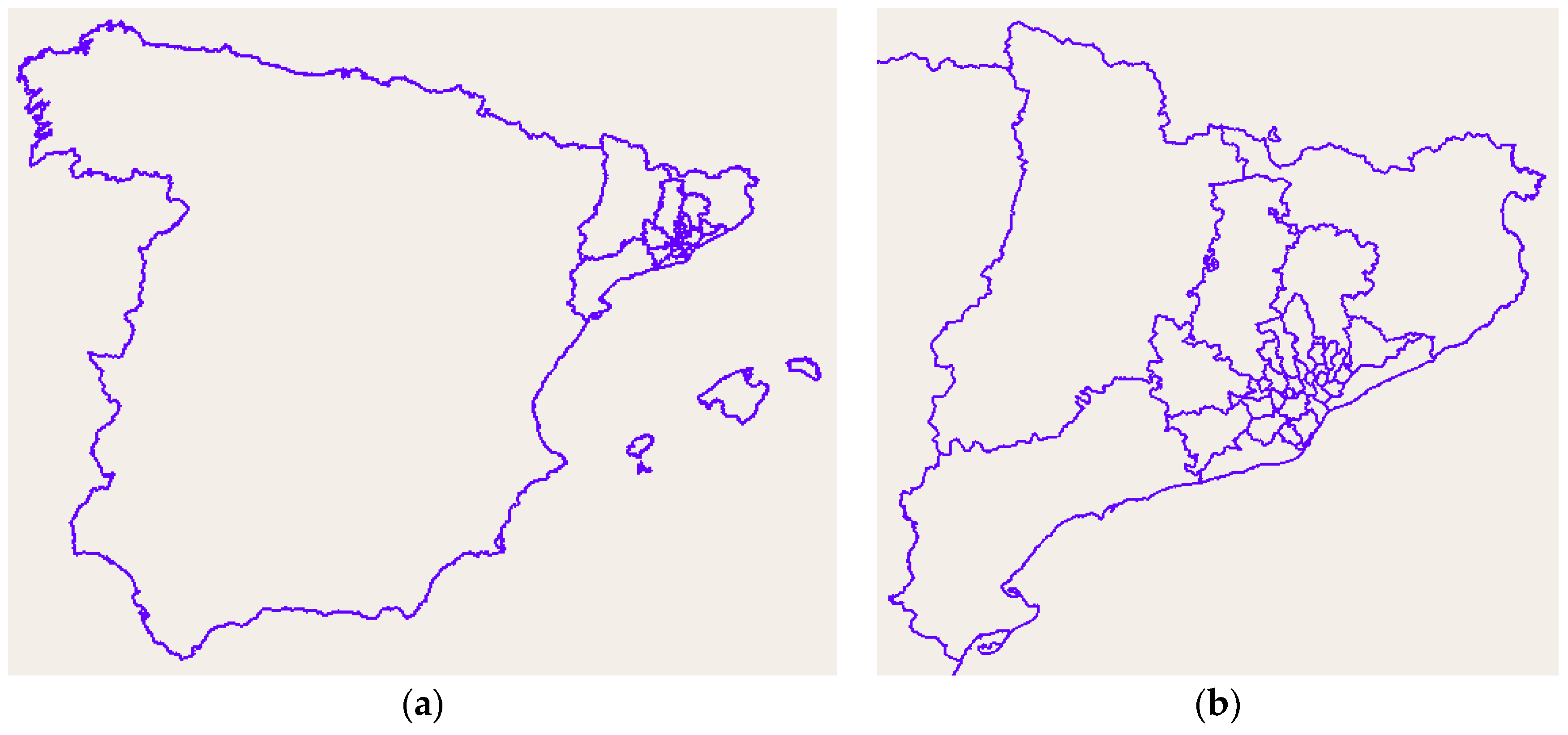
Seventeen (17) municipalities were directly affected by the layout of the different considered corridors. All 17 belonged to the province of Barcelona (Spain). However, as the study area obviously could not be limited to these municipalities, we extended it to a much larger territorial area that included the entire province of Barcelona, the neighboring provinces, and the rest of Spain.
Therefore, we defined two distinct areas:
- The internal area, which incorporated the areas on which the new infrastructure had a direct impact. This area included the municipalities directly affected by the new infrastructure and almost the entire Metropolitan Area of Barcelona.
- The external area, which incorporated some areas that supported penetration or crossing trips and usually contained more than one municipality. In the external area, we had large areas that modeled long-distance relationships in the corridor, such as trips from the Mediterranean area or Portugal to Europe or Girona.
The model consisted of 38 zones (34 internal zones plus four external macro zones), with municipal disaggregation in the area most directly influenced by the new highway, and with less detail when moving away from the area of action. All areas were composed of individual municipalities or aggregations thereof. The final zonification set is shown in Figure 1.
3.2. Determining the Basic Origin/Destination Matrix
The main source of data used in the project was anonymized mobile phone data from a network operator with an important market share of total users in Spain. To do so, information on the geolocated positions of mobile devices was gathered and recorded during March, 2018. The study population consisted of residents of Spain over 16 years old. The resulting data from this process were: four origin/destination matrices for light vehicles (with different travel reasons) and one origin/destination matrix for heavy vehicles on an average working day.
After adding the different travel reasons, a global origin/destination matrix was obtained for an average working day. Finally, based on data collected from the Movilia survey [63], we noted that the proportion of private vehicle travel on a working day was 40.6%, and that the average occupancy of vehicles was 1.22 people/vehicle on a working day. Taking into account all of these corrective elements, the final base matrices of light and heavy vehicles were obtained for the 38 considered zones. These tables were found to yield values similar to those obtained in the Movilia survey for the province of Barcelona, which gave us some confidence in the reliability of the process.
However, when applying these matrices to the network model, the traffic values recorded at the actual metering stations were not accurately reproduced. Therefore, we needed to make one last adjustment after developing the offer model (or network model).
4. Methodological Application
This section describes the particularities of the methodology that we used for the modeling in the case study. We differentiate between an offer model (a model of the road network on which the future highway is framed) and an assignment traffic model (consisting of a choice model with multiple paths according to the generalized cost).
4.1. Network Model
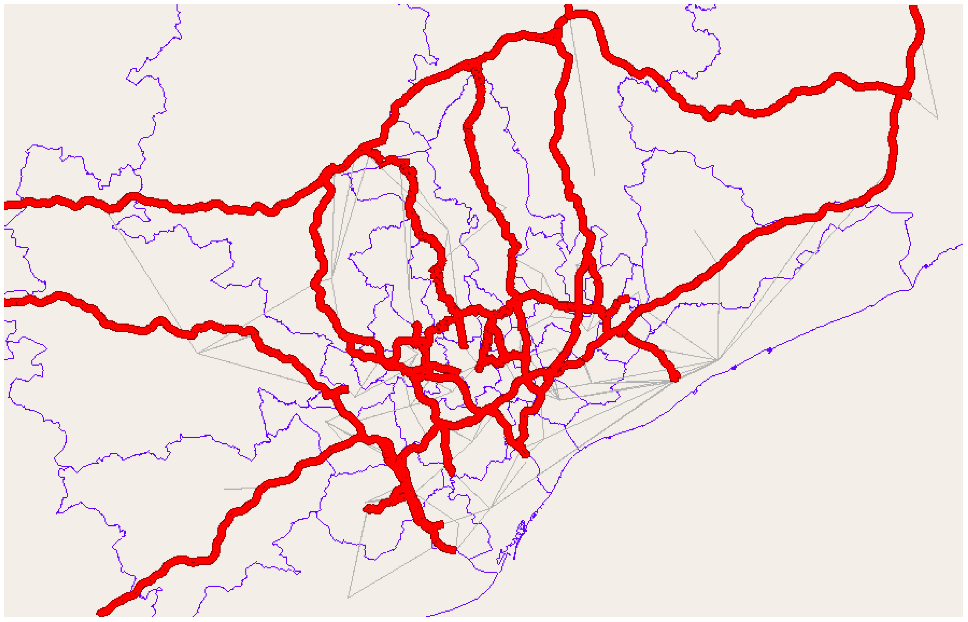
The offer model consists of a representative structure of the characteristics of the road network on which the travel matrices assignment was to be carried out. We included, as prescribed by Spanish regulations [64], all of the sections of roads belonging to corridors, from which the new road could take a significant amount of traffic, all of the sections of roads that connected the new road with alternative corridors, all of the roads that crossed the new road, and all of the connections to the traffic generation/attraction centers in the immediate area.
In other words, all of the main types of road infrastructure included in the new road’s area of influence were modeled. The scenario was complemented by the inclusion of other roads of the province of Barcelona that could potentially be in competition with the new infrastructure or may have influenced the results of the model. Furthermore, sections where movement was free were distinguished from those where a toll was applied. This incorporated an additional cost into the latter sections depending on the travelled distance.
Figure 2 shows the explanatory graph of the modeled network and the connections of the centroids on it.
In total, the modeled network consisted of 1232 sections and 519 intersections and had a total length of 1593 km (3251 km if we divided the roads by lane). Considering that the total length of the road network of the province of Barcelona was 3929 km during the same period, these data reflect the high degree of detail achieved in this study.
4.2. Traffic Assignment Model
The network model was implemented using the AIMSUN software. In this case, we used macro-simulation tools, as they have been adapted for studies in which the size of the study area is large. Each section of the network was delineated in this software from the basic information contained in the OpenStreetMap platform [65], updating the new or modified infrastructures with respect to it if necessary. The generalized cost of each section was determined using a function that considered the economic cost, the cost of spent time, and other variables, such as toll rates, if needed. The general expression of the unit generalized cost was:
where SVT is the subjective value of time. The average value of time was extracted from the Spanish regulations [66], which set a value of 23.03 euros/h for the year 2013, which we updated in accordance with the official Euribor [67].
The model assigned both types of trips—light vehicle trips and heavy vehicle trips—together to the network by applying an equivalence factor, which, in our study, was initially equal to 3.0, as this value corresponded to undulating terrain in the Highway Capacity Manual [68]. The network was simulated over various assignment models, and the results obtained with each of them were compared with the actual data from the existing metering stations.
5. Results
In this section, we compare the assignment models described in Section 2 in order to initiate a brief discussion on the quality of the different alternatives. Specifically, we performed experiments with five types of static traffic assignment (all-or-nothing, stochastic assignment with a simulation-based method, the method of successive averages (MSA), incremental assignment, and user equilibrium, applying the Frank and Wolfe algorithm). We compare the results obtained with each of these methodologies with the traffic data that were actually measured by the detectors in the network. We also qualitatively assess the ability of each methodology to estimate the traffic flow in the modeled network. To this end, we followed the guidelines established by Spanish legislation [64], which indicate that a valid model satisfies two conditions:
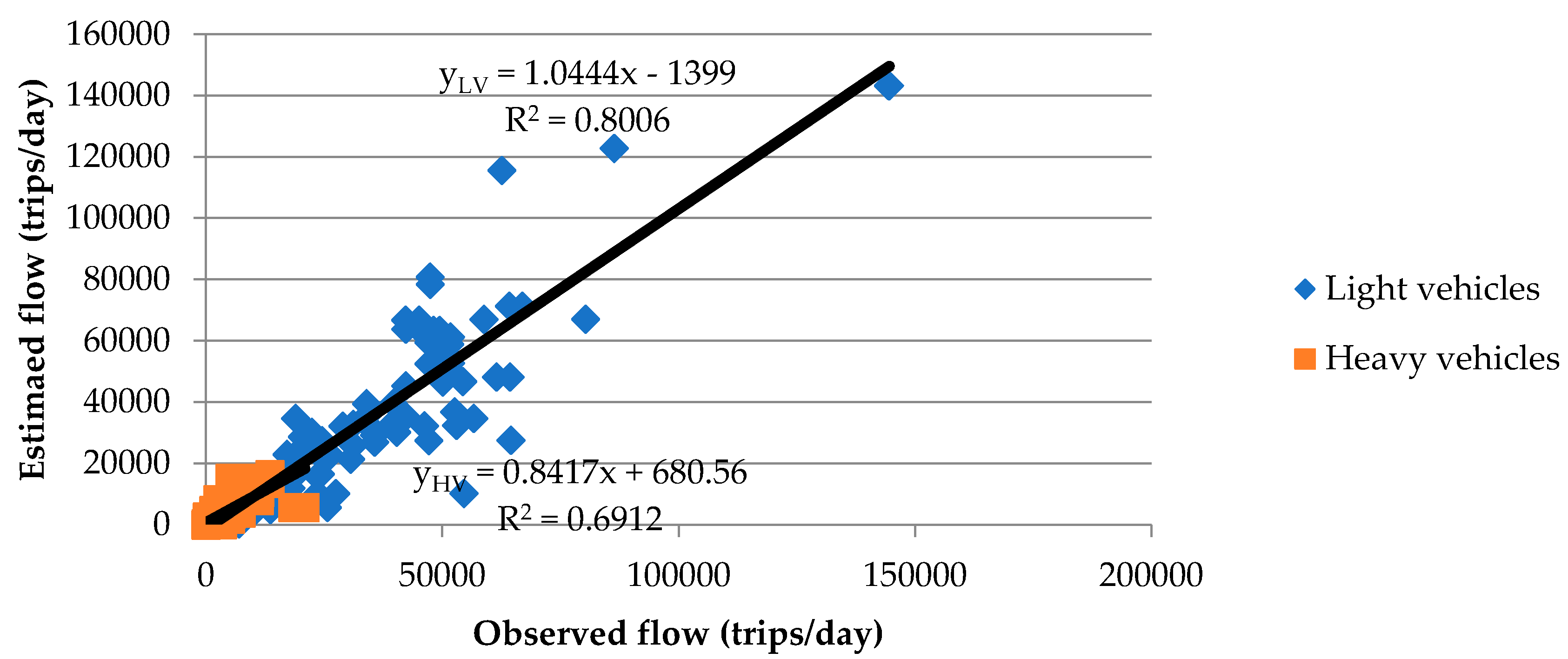
- Regression analysis. A scatter plot should be developed containing the pairs of traffic volume values obtained in each section by the model (vertical axis) and by the actual observations in metering stations (horizontal axis). Above it, a regression line must be adjusted, where the slope value should be close to 1, the intercept value on the vertical axis should be close to 0 (compared with the analyzed traffic volume ranges), and the coefficient of determination R2 should be greater than 0.7.
- Root–mean–square error (RMSE) index. The total set of observations should be divided into two groups: a “contrast” sample containing at least 10% of the values and a sample containing the rest of the values. For each group, the following indicator should be calculated, and the values in all cases should be less than 30%:where Ei is the estimated flow by the model, Oi is the observed flow in the metering station, and N is the number of observations. In our case study, the data were divided into a sample containing 29 observations (representing 28% of the total data) and a sample containing the remaining 73 observations. These proportions were used in all considered models.
5.1. All-or-Nothing Assignment
By comparing the data recorded by the metering stations with those estimated by the model, we obtained Figure 3. A regression analysis was performed between the observed and the estimated values. In Figure 3, the estimated values are shown on the vertical axis and the observed ones are shown on the horizontal axis. We found an R2 coefficient of 80.1% for light vehicles and an R2 coefficient of 69.1% for heavy vehicles. Since the value for heavy vehicles was less than 0.7 [64], this methodology can be directly discarded in the current case.
In addition, the RMSE index was calculated, resulting in a value of 27.6% for the sample of 29 observations, and a value of 43.3% for the sample of 73 observations. These results were also inadmissible [59], so we again arrived at the above conclusion.
5.2. Stochastic Assignment with a Simulation-Based Method
For the application of this methodology, we tested seven different utility functions. All of these functions were dependent on the generalized cost of travel and were calculated according to Equation (6) with a 95% level of confidence. These functions are shown in Table 1.
After comparing the data recorded in the metering station with the estimated values from the model, the results shown in Table 2 were obtained by a regression analysis. Table 2 shows that, in general terms, this methodology did not allow us to obtain a sufficient degree of approximation to the actual situation. Only the U2d utility function yielded admissible R2 coefficients [64]. Table 3 contains the results of the calculation of the RMSE indices for each considered utility function. In this case, there was no utility function that yielded values lower than 30% in all cases. Therefore, this methodology should also be discarded in the current case study.
5.3. Incremental Assignment
For this methodology, we tested six different configurations. In the first five configurations, the demand was divided equally—specifically, into 2, 3, 4, 5, and 10 parts, respectively. In the sixth configuration, we used the scheme proposed by Ortúzar and Willumsen [51] with declining proportions (40%–30%–20%–10%).
Similar to the previous cases, after comparing the data recorded by the metering stations with those estimated using the model, the results shown in Table 4 were obtained by a regression analysis. Table 4 shows that all of the considered schemes yielded admissible R2 coefficients [64]. On the other hand, Table 5 shows the results of the calculation of the RMSE indices in each analyzed case. This time, we can see that only homogeneous partitions with four or more divisions yielded values less than 30%, so they were the only permissible ones [64]. Therefore, this methodology can be accepted, but only in the case of four or more homogeneous partitions.
5.4. Method of Successive Averages (MSA)
For this methodology, we tested five different configurations with a maximum number of 5, 10, 20, 50, and 100 iterations to determine the value needed to achieve the required level of detail [64].
Table 6 shows the results of the regression analysis. The results showed that all of the considered schemes yielded admissible R2 coefficients [64]. Table 7 shows the evolution of the RMSE indices based on the number of iterations. From Table 7, we can see that all configurations with 10 or more iterations yielded permissible values [64].
Finally, Figure 4 shows a summary of the evolution of these indices based on the number of iterations. We can see there that the level of accuracy increased rapidly over the first several iterations, and then remained practically stagnant even though the number of iterations significantly increased.
5.5. User Equilibrium Using the Frank and Wolfe Algorithm
As in the previous case, the main issue to consider was the maximum number of iterations with which to limit the process. Again, we tested five different configurations with a maximum number of 5, 10, 20, 50, and 100 iterations.
After comparing the data recorded by the metering stations with those estimated using the model, the results shown in Table 8 were obtained by a regression analysis. Table 9 shows the evolution of the RMSE indices based on the number of iterations. Table 8 and Table 9 show that all of the considered schemes yielded admissible R2 coefficients and that all configurations, even the one that only had five iterations, yielded adequate RMSE values [64].
Finally, Figure 5 shows that the level of accuracy increased even more rapidly over the first several iterations than in the MSA algorithm, and then remained practically stagnant even though the number of iterations significantly increased. This finding was consistent with those of Arezki and Van Vliet [59].
6. Discussion and Conclusions
From our analysis, we can draw the following conclusions:
- The all-or-nothing and stochastic assignment methods are inadmissible in this particular case study. In our study, we did not obtain the same outcome as Chen and Pan [69], who concluded that stochastic algorithms can produce similar results to the UE and MSA. This may be due to the size of the simulated network; the examples they used were small in size, while we analyzed a large area. Further research is needed to verify this point.
- The incremental assignment algorithms are valid only when they have four or more demand partitions of equal size; thus, no individual partition can exceed 25% of the total.
- The method of successive averages (MSA) algorithm is valid only when working with more than 10 iterations. This result is consistent with those of Ameli et al. [1], who found that this method is good for small- and medium-sized networks, but is not the fastest one when estimating the traffic flow in a large network.
- Finally, the user equilibrium methods (approximated by the Frank and Wolfe algorithm) were found to be valid in all of the considered cases (five or more iterations).
Table 10 shows a summary of the results obtained using those methodologies that were found to be valid for the case study.
From the results, we can conclude that the MSA and UE yield practically the same results when we have a sufficiently high number of iterations [59]. However, for lower numbers of iterations, the results of the UE algorithm are clearly better. The incremental allocation method provides a significantly lower level of detail.
Therefore, we recommend the use of user equilibrium methodologies. To speed up the process, approximation with the Frank and Wolfe algorithm could be performed. This recommendation is in line with the results of Denoyelle et al. [70], who determined, by applying numerical simulation techniques, that this method is versatile and superior to other methodologies.
However, as Bliemer et al. [71] note, planners have to evaluate a methodology’s applicability in terms of both its adjustment to real-world data and its computational flexibility and speed. In our case study, the Frank and Wolfe algorithm was found to satisfy all of these criteria. We can infer that a network’s size is a crucial variable to take into account when choosing a method [40,41,44,69,71].
To finish, we want to make a note about the limitations of this study and its scientific and practical implications. In this study, we used five different types of methods to estimate the traffic flow in a large network and compared the results with real-world data. These five methods were the ones included in the employed software. It would be interesting to use other methodologies, or even a higher number of different configurations within the considered ones. In addition, we determined whether the models complied with the Spanish regulations [64], since their verification, through the R2 and the RMSE indices, is a prerequisite of their use in our geographical area. However, it would have been interesting to use other goodness-of-fit indicators, or even to develop new ones, to enhance our knowledge of the adjustment of each methodology to real-world data. These are possible lines of future research in this field.
Regarding scientific and practical implications, we want to note that the results obtained in this study can be considered to be valid for both the case study and other areas with similar characteristics. However, although they cannot be directly extrapolated to different cases, it may be possible to develop a similar methodology that allows, under the same conditions, for the selection of the optimal assignment method in eacvv cfdh case. The results of this study and the employed procedure may be useful to researchers in the field of computer simulation and planners who apply these methodologies in similar cases.
Funding
This research was carried out using funds provided under the Research Contract entitled “Simulación y Análisis de Tráfico dentro del Estudio Informativo de la Autovía Orbital B-40” (Simulation and Traffic Analysis within the Study Report of the B-40 Orbital Highway) between GPYO Innova, S.L. and the University of Burgos (Spain) with reference number W24T06.
Conflicts of Interest
The authors declare no conflicts of interest. The funders participated in the collection of data and agree with the decision to publish the results.
References
- Ameli, M.; Lebacque, J.; Leclercq, L. Cross-comparison of convergence algorithms to solve trip-based dynamic traffic assignment problems. Comput. Civ. Infrastruct. Eng. 2020, 35, 219–240. [Google Scholar] [CrossRef]
- Ameli, M.; Lebacque, J.-P.; Leclercq, L. Improving traffic network performance with road banning strategy: A simulation approach comparing user equilibrium and system optimum. Simul. Model. Pr. Theory 2020, 99, 101995. [Google Scholar] [CrossRef]
- Bagdasar, O.; Popovici, N.; Berry, S. Traffic assignment: On the interplay between optimization and equilibrium problems. Optimization 2020, 1–18. [Google Scholar] [CrossRef]
- Tan, H.; Du, M.; Jiang, X.; Chu, Z. The Combined Distribution and Assignment Model: A New Solution Algorithm and Its Applications in Travel Demand Forecasting for Modern Urban Transportation. Sustainability 2019, 11, 2167. [Google Scholar] [CrossRef] [Green Version]
- Zhang, T.; Yang, Y.; Cheng, G.; Jin, M. A Practical Traffic Assignment Model for Multimodal Transport System Considering Low-Mobility Groups. Mathematics 2020, 8, 351. [Google Scholar] [CrossRef] [Green Version]
- Wang, Y.; Szeto, W.; Han, K.; Friesz, T.L. Dynamic traffic assignment: A review of the methodological advances for environmentally sustainable road transportation applications. Transp. Res. Part B Methodol. 2018, 111, 370–394. [Google Scholar] [CrossRef]
- Mao, X.; Wang, J.; Yuan, C.; Yu, W.; Gan, J. A Dynamic Traffic Assignment Model for the Sustainability of Pavement Performance. Sustainability 2018, 11, 170. [Google Scholar] [CrossRef] [Green Version]
- Pel, A.J.; Chaniotakis, E. Stochastic user equilibrium traffic assignment with equilibrated parking search routes. Transp. Res. Part B Methodol. 2017, 101, 123–139. [Google Scholar] [CrossRef]
- Al-Ahmadi, H.; Jamal, A.; Reza, I.; Assi, K.; Ahmed, S.A. Using Microscopic Simulation-Based Analysis to Model Driving Behavior: A Case Study of Khobar-Dammam in Saudi Arabia. Sustainability 2019, 11, 3018. [Google Scholar] [CrossRef] [Green Version]
- Wei, L.; Xu, J.; Lei, T.; Li, M.; Liu, X.; Li, H. Simulation and Experimental Analyses of Microscopic Traffic Characteristics under a Contraflow Strategy. Appl. Sci. 2019, 9, 2651. [Google Scholar] [CrossRef] [Green Version]
- Long, J.; Szeto, W.; Du, J.; Wong, C.P. A dynamic taxi traffic assignment model: A two-level continuum transportation system approach. Transp. Res. Part B Methodol. 2017, 100, 222–254. [Google Scholar] [CrossRef] [Green Version]
- Bischoff, J.; Maciejewski, M. Simulation of City-wide Replacement of Private Cars with Autonomous Taxis in Berlin. Procedia Comput. Sci. 2016, 83, 237–244. [Google Scholar] [CrossRef] [Green Version]
- Heilig, M.; Hilgert, T.; Mallig, N.; Kagerbauer, D.-I.M.; Vortisch, P. Potentials of Autonomous Vehicles in a Changing Private Transportation System—A Case Study in the Stuttgart Region. Transp. Res. Procedia 2017, 26, 13–21. [Google Scholar] [CrossRef]
- Poulhès, A.; Berrada, J. User assignment in a smart vehicles’ network: Dynamic modelling as an agent-based model. Transp. Res. Procedia 2017, 27, 865–872. [Google Scholar] [CrossRef]
- Poulhès, A.; Berrada, J. Single vehicle network versus dispatcher: User assignment in an agent-based model. Transp. A Transp. Sci. 2020, 16, 270–292. [Google Scholar] [CrossRef]
- Liu, T.; Ceder, A. Integrated Public Transport Timetable Synchronization and Vehicle Scheduling with Demand Assignment: A Bi-objective Bi-level Model Using Deficit Function Approach. Transp. Res. Procedia 2017, 23, 341–361. [Google Scholar] [CrossRef]
- Eltved, M.; Nielsen, O.A.; Rasmussen, T.K. An assignment model for public transport networks with both schedule- and frequency-based services. EURO J. Transp. Logist. 2019, 8, 769–793. [Google Scholar] [CrossRef]
- Cats, O.; Hartl, M. Modelling public transport on-board congestion: Comparing schedule-based and agent-based assignment approaches and their implications. J. Adv. Transp. 2016, 50, 1209–1224. [Google Scholar] [CrossRef] [Green Version]
- Nuzzolo, A.; Comi, A. Advanced Public Transport and ITS: New modelling challenges. Transp. A Transp. Sci. 2016, 12, 1–51. [Google Scholar] [CrossRef]
- Lin, D.-Y.; Fang, J.-H.; Huang, K.-L. Passenger assignment and pricing strategy for a passenger railway transportation system. Transp. Lett. 2017, 11, 320–331. [Google Scholar] [CrossRef]
- Xu, G.; Zhao, S.; Shi, F.; Zhang, F. Cell transmission model of dynamic assignment for urban rail transit networks. PLoS ONE 2017, 12, e0188874. [Google Scholar] [CrossRef] [PubMed] [Green Version]
- Gao, S.; Wu, Z. Modeling Passenger Flow Distribution Based on Travel Time of Urban Rail Transit. J. Transp. Syst. Eng. Inf. Technol. 2011, 11, 124–130. [Google Scholar] [CrossRef]
- Venturini, G.; Iris, C.; Kontovas, C.; Larsen, A. The multi-port berth allocation problem with speed optimization and emission considerations. Transp. Res. Part D Transp. Environ. 2017, 54, 142–159. [Google Scholar] [CrossRef] [Green Version]
- Iris, C.; Pacino, D.; Røpke, S.; Larsen, A. Integrated Berth Allocation and Quay Crane Assignment Problem: Set partitioning models and computational results. Transp. Res. Part E Logist. Transp. Rev. 2015, 81, 75–97. [Google Scholar] [CrossRef] [Green Version]
- Li, S.; Jia, S. The seaport traffic scheduling problem: Formulations and a column-row generation algorithm. Transp. Res. Part B Methodol. 2019, 128, 158–184. [Google Scholar] [CrossRef]
- Han, Y.; Lee, L.H.; Chew, E.P.; Tan, K.C. A yard storage strategy for minimizing traffic congestion in a marine container transshipment hub. OR Spectr. 2008, 30, 697–720. [Google Scholar] [CrossRef]
- Iris, C.; Christensen, J.M.; Pacino, D.; Røpke, S. Flexible ship loading problem with transfer vehicle assignment and scheduling. Transp. Res. Part B Methodol. 2018, 111, 113–134. [Google Scholar] [CrossRef] [Green Version]
- Ganic, E.; Babić, O.; Cangalovic, M.; Stanojevic, M. Air traffic assignment to reduce population noise exposure using activity-based approach. Transp. Res. Part D Transp. Environ. 2018, 63, 58–71. [Google Scholar] [CrossRef]
- Ho-Huu, V.; Ganić, E.; Hartjes, S.; Babić, O.; Curran, R. Air traffic assignment based on daily population mobility to reduce aircraft noise effects and fuel consumption. Transp. Res. Part D Transp. Environ. 2019, 72, 127–147. [Google Scholar] [CrossRef]
- Starita, S.; Strauss, A.K.; Fei, X.; Jovanović, R.; Ivanov, N.; Pavlović, G.; Fichert, F. Air Traffic Control Capacity Planning Under Demand and Capacity Provision Uncertainty. Transp. Sci. 2020. [Google Scholar] [CrossRef]
- Yu, X.; Wang, H.; Ge, Z.; Guo, J. Traffic assignment model for combined mode with travel condition constraints. Int. J. Mod. Phys. B 2020, 34, 2050003. [Google Scholar] [CrossRef]
- Pi, X.; Ma, W.; Qian, Z.S. A general formulation for multi-modal dynamic traffic assignment considering multi-class vehicles, public transit and parking. Transp. Res. Part C Emerg. Technol. 2019, 104, 369–389. [Google Scholar] [CrossRef]
- Macedo, E.; Tomás, R.; Fernandes, P.; Coelho, M.C.; Bandeira, J.M. Quantifying road traffic emissions embedded in a multi-objective traffic assignment model. Transp. Res. Procedia 2020, 47, 648–655. [Google Scholar] [CrossRef]
- Jiang, Y.; Szeto, W.; Long, J.; Han, K. Multi-class dynamic traffic assignment with physical queues: Intersection-movement-based formulation and paradox. Transp. A Transp. Sci. 2016, 12, 878–908. [Google Scholar] [CrossRef] [Green Version]
- Dimitrov, S.; Ceder, A.; Chowdhury, S.; Monot, M. Modeling the interaction between buses, passengers and cars on a bus route using a multi-agent system. Transp. Plan. Technol. 2017, 40, 592–610. [Google Scholar] [CrossRef]
- Zhang, L.; Yang, D.; Ghader, S.; Carrion, C.; Xiong, C.; Rossi, T.F.; Milkovits, M.; Mahapatra, S.; Barber, C. An Integrated, Validated, and Applied Activity-Based Dynamic Traffic Assignment Model for the Baltimore-Washington Region. Transp. Res. Rec. J. Transp. Res. Board 2018, 2672, 45–55. [Google Scholar] [CrossRef]
- Shafiei, S.; Gu, Z.; Saberi, M. Calibration and validation of a simulation-based dynamic traffic assignment model for a large-scale congested network. Simul. Model. Pract. Theory 2018, 86, 169–186. [Google Scholar] [CrossRef]
- Zhu, Z.; Xiong, C.; Chen, X.; He, X.; Zhang, L. Integrating mesoscopic dynamic traffic assignment with agent-based travel behavior models for cumulative land development impact analysis. Transp. Res. Part C Emerg. Technol. 2018, 93, 446–462. [Google Scholar] [CrossRef]
- Kucharski, R.; Gentile, G. Simulation of rerouting phenomena in Dynamic Traffic Assignment with the Information Comply Model. Transp. Res. Part B Methodol. 2019, 126, 414–441. [Google Scholar] [CrossRef]
- Zhang, H.; Seshadri, R.; Prakash, A.A.; Pereira, F.C.; Antoniou, C.; Ben-Akiva, M.E. Improved Calibration Method for Dynamic Traffic Assignment Models: Constrained Extended Kalman Filter. Transp. Res. Rec. J. Transp. Res. Board 2017, 2667, 142–153. [Google Scholar] [CrossRef] [Green Version]
- Prakash, A.A.; Seshadri, R.; Antoniou, C.; Pereira, F.C.; Ben-Akiva, M.E. Reducing the Dimension of Online Calibration in Dynamic Traffic Assignment Systems. Transp. Res. Rec. J. Transp. Res. Board 2017, 2667, 96–107. [Google Scholar] [CrossRef]
- Du, L.; Song, G.; Wang, Y.; Huang, J.; Ruan, M.; Yu, Z. Traffic Events Oriented Dynamic Traffic Assignment Model for Expressway Network: A Network Flow Approach. IEEE Intell. Transp. Syst. Mag. 2018, 10, 107–120. [Google Scholar] [CrossRef]
- Lin, Y.-Z.; Chen, W.-H. A simulation-based multiclass, multimodal traffic assignment model with departure time for evaluating traffic control plans of planned special events. Transp. Res. Procedia 2017, 25, 1352–1379. [Google Scholar] [CrossRef]
- Batista, S.F.A.; Leclercq, L. Regional Dynamic Traffic Assignment Framework for Macroscopic Fundamental Diagram Multi-regions Models. Transp. Sci. 2019, 53, 1563–1590. [Google Scholar] [CrossRef]
- Bagdasar, O.; Berry, S.; O’Neill, S.; Popovici, N.; Raja, R. Traffic assignment: Methods and simulations for an alternative formulation of the fixed demand problem. Math. Comput. Simul. 2019, 155, 360–373. [Google Scholar] [CrossRef] [Green Version]
- Cascetta, E. Transportation Systems Analysis: Models and Applications, 2nd ed.; Springer: Berlin/Heidelberg, Germany, 2009. [Google Scholar]
- Cantarella, G.E. A General Fixed-Point Approach to Multimode Multi-User Equilibrium Assignment with Elastic Demand. Transp. Sci. 1997, 31, 107–128. [Google Scholar] [CrossRef]
- Cantarella, G.; Watling, D.; de Luca, S.; Di Pace, R. Dynamics and Stochasticity in Transportation Systems, Tools for Transportation Network Modeling, 1st ed.; Elsevier: Amsterdam, The Netherlands, 2019. [Google Scholar]
- Cantarella, G.E.; Carteni, A.; De Luca, S. Stochastic equilibrium assignment with variable demand: Theoretical and implementation issues. Eur. J. Oper. Res. 2015, 241, 330–347. [Google Scholar] [CrossRef]
- Cantarella, G.E.; De Luca, S.; Di Gangi, M.; Di Pace, R. Approaches for solving the stochastic equilibrium assignment with variable demand: Internal vs. external solution algorithms. Optim. Methods Softw. 2014, 30, 338–364. [Google Scholar] [CrossRef]
- Ortúzar, J.D.; Willumsen, L.G. Modelling Transport, 4th ed.; Wiley & Sons: Hoboken, NJ, USA, 2011. [Google Scholar]
- Lee, E.S.; Oduor, P.G. Using Multi-Attribute Decision Factors for a Modified All-or-Nothing Traffic Assignment. ISPRS Int. J. Geo Inf. 2015, 4, 883–899. [Google Scholar] [CrossRef]
- Burrel, J.E. Multiple Route Assignment and its Application to Capacity Restraint. In Proceedings of the Fourth International Symposium on the Theory of Traffic Flow, Karlsruhe, Germany, 18–20 June 1968. [Google Scholar]
- Dial, R.B. A probabilistic multipath traffic assignment model which obviates path enumeration. Transp. Res. 1971, 5, 83–111. [Google Scholar] [CrossRef]
- Wardrop, J.G. Road paper. some theoretical aspects of road traffic research. Proc. Inst. Civ. Eng. 1952, 1, 325–362. [Google Scholar] [CrossRef]
- Sheffi, Y. Urban Transportation Networks; Prentice Hall: Englewood Cliff, NJ, USA, 1985. [Google Scholar]
- Smock, R.J. An iterative assignment approach to capacity restraint on arterial networks. Highw. Res. Board Bull. 1962, 347, 60–66. [Google Scholar]
- Frank, M.; Wolfe, P. An algorithm for quadratic programming. Nav. Res. Logist. Q. 1956, 3, 95–110. [Google Scholar] [CrossRef]
- Arezki, Y.; Van Vliet, D. A Full Analytical Implementation of the PARTAN/Frank–Wolfe Algorithm for Equilibrium Assignment. Transp. Sci. 1990, 24, 58–62. [Google Scholar] [CrossRef]
- Generalitat de Cataluña. Observatorio Viario de Cataluña 2014. (VIACAT); Generalitat de Cataluña: Barcelona, Spain, 2015. Available online: http://territori.gencat.cat/es/03_infraestructures_i_mobilitat/carreteres/observatori_viari_de_catalunya_viacat/publicacions_enllacos_interes/5_1_anuari_estadistic_viacat/anuari-estadistic-viacat-2014/ (accessed on 1 June 2018).
- Ministerio de Fomento. Mapa de Tráfico 2016; Ministerio de Fomento: Madrid, Spain, 2017. Available online: https://www.mitma.es/carreteras/trafico-velocidades-y-accidentes-mapa-estimacion-y-evolucion/mapas-de-trafico (accessed on 1 June 2018).
- Generalitat de Cataluña. Plan de Aforos 2016; Generalitat de Cataluña: Barcelona, Spain, 2017. Available online: http://territori.gencat.cat/ca/01_departament/documentacio/mobilitat/carreteres/pla_daforaments/ (accessed on 1 June 2018).
- Encuesta de Movilidad de las Personas Residentes en España, MOVILIA 2006/2007; Ministerio de Fomento: Madrid, Spain, 2008.
- Nota De Servicio 5/2014, Prescripciones y Recomendaciones Técnicas para la Realización de Estudios de Tráfico de los Estudios Informativos, Anteproyectos y Proyectos De Carreteras; Ministerio de Fomento: Madrid, Spain, 2014.
- OpenStreetMap. Available online: https://www.openstreetmap.org (accessed on 1 February 2018).
- Nota de Servicio 3/2014, Prescripciones y Recomendaciones Técnicas Relativas a los Contenidos Mínimos a Incluir en los Estudios de Rentabilidad de los Estudios Informativos de la Subdirección General de Estudios y Proyectos; Ministerio de Fomento: Madrid, Spain, 2014.
- Euribor. Available online: https://es.euribor-rates.eu (accessed on 1 June 2018).
- Transportation Research Board (TRB). Highway Capacity Manual HCM 2016; Transportation Research Board: NW Washington, DC, USA, 2016. [Google Scholar]
- Chen, Q.; Pan, S. Direct formulation and algorithms for the probit-based stochastic user equilibrium traffic assignment problem. Transp. Plan. Technol. 2017, 40, 1–14. [Google Scholar] [CrossRef]
- Denoyelle, Q.; Duval, V.; Peyré, G.; Soubies, E. The sliding Frank–Wolfe algorithm and its application to super-resolution microscopy. Inverse Probl. 2019, 36, 014001. [Google Scholar] [CrossRef] [Green Version]
- Bliemer, M.C.J.; Raadsen, M.P.H.; Brederode, L.J.N.; Bell, M.G.H.; Wismans, L.J.J.; Smith, M.J. Genetics of traffic assignment models for strategic transport planning. Transp. Rev. 2016, 37, 56–78. [Google Scholar] [CrossRef] [Green Version]
Figure 1.
Geographical distribution of zones. (a) The whole of Spain; (b) Catalonia in detail.

Figure 2.
The base road network.

Figure 3.
All-or-nothing assignment: regression analysis.

Figure 4.
MSA assignment: comparison by number of iterations.

Figure 5.
Equilibrium assignment: comparison by number of iterations.


Table 1.
Stochastic assignment: utility functions.
| Function | Equation |
|---|---|
| U1a | |
| U1b | |
| U1c | |
| U2a | |
| U2b | |
| U2c | |
| U2d |
Where Uijr is the utility within path r for trips from i to j and cij is the generalized cost of the trip from i to j.
Table 2.
Stochastic assignment: regression analysis.
| Utility Function | Light Vehicles | Heavy Vehicles | ||
|---|---|---|---|---|
| Equation | R2 | Equation | R2 | |
| U1a | y = 1.0312x − 753.67 | 0.7886 | y = 0.8523x + 1296.8 | 0.6146 |
| U1b | y = 1.0258x − 41.031 | 0.7808 | y = 0.889x + 1563.3 | 0.5308 |
| U1c | y = 1.02x + 553.03 | 0.7738 | y = 0.9241x + 1690 | 0.4754 |
| U2a | y = 1.7822x − 9943.3 | 0.715 | y = 0.7287x + 2677.2 | 0.2442 |
| U2b | y = 1.6037x − 7780.3 | 0.7405 | y = 0.7797x + 1954.1 | 0.4494 |
| U2c | y = 1.4134x − 5076.1 | 0.7688 | y = 0.8021x + 1578.5 | 0.5765 |
| U2d | y = 1.1243x − 975.06 | 0.7969 | y = 0.92x + 927.58 | 0.7445 |
Table 3.
Stochastic assignment: root–mean–square error (RMSE) index.
| Utility Function | Sample | Rest |
|---|---|---|
| U1a | 25.5% | 43.5% |
| U1b | 26.9% | 45.5% |
| U1c | 28.2% | 47.6% |
| U2a | 87.5% | 108.7% |
| U2b | 65.5% | 90.2% |
| U2c | 43.2% | 72.1% |
| U2d | 20.9% | 49.1% |
Table 4.
Incremental assignment: regression analysis.
| Partitions | Light Vehicles | Heavy Vehicles | ||
|---|---|---|---|---|
| Equation | R2 | Equation | R2 | |
| 2 × 50% | y = 1.0539x − 1335.1 | 0.8691 | y = 0.8557x + 610.06 | 0.7918 |
| 3 × 33% | y = 1.0528x − 1670.4 | 0.8872 | y = 0.85x + 607.36 | 0.8046 |
| 4 × 25% | y = 1.0436x − 863.34 | 0.8984 | y = 0.8692x + 559.38 | 0.8429 |
| 5 × 20% | y = 1.0345x − 642.87 | 0.9049 | y = 0.8503x + 646.15 | 0.824 |
| 10 × 10% | y = 1.0389x + 475.52 | 0.8976 | y = 0.8632x + 604.35 | 0.8466 |
| 40–30–20–10% | y = 1.0381x + 475.58 | 0.883 | y = 0.8519x + 654.53 | 0.8162 |
Table 5.
Incremental assignment: RMSE index.
| Partitions | Sample | Rest |
|---|---|---|
| 2 × 50% | 21.4% | 34.7% |
| 3 × 33% | 22.4% | 31.0% |
| 4 × 25% | 20.3% | 29.1% |
| 5 × 20% | 19.4% | 28.0% |
| 10 × 10% | 18.8% | 29.3% |
| 40–30–20–10% | 18.3% | 31.7% |
Table 6.
Method of successive averages (MSA) assignment: regression analysis.
| No Iterations | Light Vehicles | Heavy Vehicles | ||
|---|---|---|---|---|
| Equation | R2 | Equation | R2 | |
| 5 | y = 1.031x + 4306.5 | 0.864 | y = 0.8644x + 718.37 | 0.8615 |
| 10 | y = 1.0257x + 2670.5 | 0.9153 | y = 0.8799x + 602.54 | 0.8826 |
| 20 | y = 0.9967x + 2370.5 | 0.9324 | y = 0.8965x + 510.79 | 0.8866 |
| 50 | y = 0.9872x + 1888.3 | 0.9341 | y = 0.9095x + 440.84 | 0.888 |
| 100 | y = 0.9861x + 1671.5 | 0.9335 | y = 0.9143x + 412.01 | 0.8893 |
Table 7.
MSA assignment: RMSE index.
| No Iterations | Sample | Rest |
|---|---|---|
| 5 | 21.6% | 37.1% |
| 10 | 15.5% | 28.8% |
| 20 | 14.3% | 24.3% |
| 50 | 14.9% | 23.0% |
| 100 | 15.3% | 22.8% |
Table 8.
Equilibrium assignment: regression analysis.
| No Iterations | Light Vehicles | Heavy Vehicles | ||
|---|---|---|---|---|
| Equation | R2 | Equation | R2 | |
| 5 | y = 0.9809x + 3849.9 | 0.8889 | y = 0.8544x + 733.41 | 0.8417 |
| 10 | y = 1.0006x + 2551.3 | 0.9224 | y = 0.8867x + 578.03 | 0.8784 |
| 20 | y = 0.9917x + 2008 | 0.9324 | y = 0.908x + 467.01 | 0.8876 |
| 50 | y = 0.9749x + 2019.3 | 0.9329 | y = 0.907x + 444.57 | 0.8874 |
| 100 | y = 0.9784x + 1752.4 | 0.9325 | y = 0.9143x + 410.07 | 0.8893 |
Table 9.
Equilibrium assignment: RMSE index.
| No Iterations. | Sample | Rest |
|---|---|---|
| 5 | 17.5% | 29.8% |
| 10 | 15.5% | 25.8% |
| 20 | 14.8% | 23.6% |
| 50 | 15.4% | 22.7% |
| 100 | 15.6% | 22.7% |
Table 10.
Comparison of results obtained with valid methodologies.
| Algorithm | R2 Index | RMSE Index | |||
|---|---|---|---|---|---|
| Light Vehicles | Heavy Vehicles | Sample | Rest | ||
| Incremental assignment | 4 × 25% | 0.8984 | 0.8429 | 20.3% | 29.1% |
| 5 × 20% | 0.9049 | 0.824 | 19.4% | 28.0% | |
| 10 × 10% | 0.8976 | 0.8466 | 18.8% | 29.3% | |
| MSA | 10 iterations | 0.9153 | 0.8826 | 15.5% | 28.8% |
| 20 iterations | 0.9324 | 0.8866 | 14.3% | 24.3% | |
| 50 iterations | 0.9341 | 0.888 | 14.9% | 23.0% | |
| 100 iterations | 0.9335 | 0.8893 | 15.3% | 22.8% | |
| User equilibrium | 5 iterations | 0.8889 | 0.8417 | 17.5% | 29.8% |
| 10 iterations | 0.9224 | 0.8784 | 15.5% | 25.8% | |
| 20 iterations | 0.9324 | 0.8876 | 14.8% | 23.6% | |
| 50 iterations | 0.9329 | 0.8874 | 15.4% | 22.7% | |
| 100 iterations | 0.9325 | 0.8893 | 15.6% | 22.7% | |
© 2020 by the author. Licensee MDPI, Basel, Switzerland. This article is an open access article distributed under the terms and conditions of the Creative Commons Attribution (CC BY) license (http://creativecommons.org/licenses/by/4.0/).
Share and Cite
MDPI and ACS Style
Rojo, M. Evaluation of Traffic Assignment Models through Simulation. Sustainability 2020, 12, 5536. https://doi.org/10.3390/su12145536
AMA Style
Rojo M. Evaluation of Traffic Assignment Models through Simulation. Sustainability. 2020; 12(14):5536. https://doi.org/10.3390/su12145536
Chicago/Turabian StyleRojo, Marta. 2020. "Evaluation of Traffic Assignment Models through Simulation" Sustainability 12, no. 14: 5536. https://doi.org/10.3390/su12145536
Note that from the first issue of 2016, this journal uses article numbers instead of page numbers. See further details here.