A New Climate Nowcasting Tool Based on Paleoclimatic Data

Abstract

Atmospheric pollutants and environmental indicators are often used to reconstruct historic atmospheric pollution from peat, as it accumulates over time by decomposing plant material, thus recording a history of air pollution. In the present study, three key parameters related to the peat bogs’ surface wetness dynamics in European Russia during the Holocene were investigated using modern statistical analysis. These parameters are: (i) the water table depth (WTD) in relation to the surface, which is reconstructed based on the community structure of the subfossil testate amoeba assemblages; (ii) the peat humification estimated as absorption of alkaline extract that directly reflects moisture at which the peat was formed; (iii) the Climate Moisture Index (CMI) and the Aridity Index derived from pollen-based reconstructions of the mean annual temperature and precipitation and classifying moisture conditions as the ratio between available annual precipitation and potential land surface evapotranspiration. All these parameters provide useful information about the paleoclimate (atmospheric moisture component) dynamics. High values of WTD and peat humification appear to comply with Gutenberg–Richter law. It is noteworthy that this law also seems to reproduce the high values of the modeled climate moisture and aridity indices. The validity of this new result is checked by replacing “conventional time” with “natural time”. On this basis, a new nowcasting tool is developed to more accurately estimate the average waiting time for the extreme values of these climate parameters. This will help to understand climate variability better to address emerging development needs and priorities by implementing empirical studies of the interactions between climatic effects, mitigation, adaptation, and sustainable growth.

1. Introduction

A better understanding of the climate–land surface interaction in the past and present is a very important issue, especially for predicting its future changes. Mathematical models can be very useful in deriving the key components of the energy, water, and carbon budgets of the ground surface and to predict the spatial and temporal variability of surface evapotranspiration, surface moisture and runoff, carbon uptake and release, etc. [1,2]. Over the past few decades, many process-based and statistical models of different levels of complexity have been developed and implemented in various climatological, hydrological, and ecological studies [3,4]. While process-based models use mathematical representations of physical and biological processes on the land surface–atmosphere interface, statistical models apply mathematically-formalized ways to derive reality using statistical methods. Recent progress in the modeling of paleo ecological processes has been made using advanced mathematical tools and sophisticated models of statistical physics developed based on long-term biological data [5,6,7]. Natural time and multifractal analyses are core concepts for studies aimed at building nowcasting models [8,9,10].

The paleo ecological records archived in various types of deposits represent a valuable tool for long-term modeling of biosphere dynamics and past climate change. Peatlands, with their gradual and consistent accretion of deposits, make these ecosystems an excellent medium for paleoecology with a range of biological remains preserved. Peat proxies are capable of indicating a variety of aspects of Holocene climate change [11,12]. Ombrotrophic (‘rain-fed’) peatlands receive all their moisture directly from the atmosphere and are, therefore, particularly sensitive to changing hydroclimate. It is believed that the peatland surface wetness may be a useful indicator of climate, and in the last two decades, the reconstructions of Holocene climate by peats have proliferated [13,14].

Recently, we applied biological (remains of pollen and testate amoebae in peat) and physicochemical (peat humification) proxies to reconstruct surface wetness dynamics during the Holocene in two peatlands in the East European Plain [15,16,17].

The present study aims to investigate the long-term variability of the reconstructed values of peatland surface wetness to develop a new nowcasting tool for evaluating the average waiting time in which these parameters achieve extreme values. With the term nowcasting of these parameters, we refer to the use of their data to estimate the current dynamical state of these parameters. In other words, nowcasting differs from forecasting in that its objective is to assess the current state of these parameters and not the probability of future extreme values, which is the goal of forecasting [18,19]. This will reduce losses to climate-related risks enhancing sustainability.

2. Data and Methods

2.1. Data

The dataset used in the present analysis contains parameters that reflect the long-term dynamics of surface wetness and peat humification in two peat bogs situated in the East European Plain (namely Klukva [15,16] and Staroselsky Mokh [17]) during the Holocene. Due to the fact that peat bogs receiving water only from the atmospheric via precipitation, surface wetness can be a very good indicator to reflect surface moisture conditions.

To describe the surface wetness, we used in our study three key parameters: (i) the water table depth (WTD) in relation to the surface (i.e., the depth of water below the bog surface), which was reconstructed based on the community structure of the subfossil testate amoeba assemblages, using the transfer function developed by Tsyganov et al. [20]; (ii) the peat humification estimated as absorption of alkaline extract that directly reflects the moisture in which the peat was formed [21]; (iii) the Climate Moisture Index (CMI) suggested by Willmott and Feddema [22] and the Aridity Index obtained using pollen-based reconstructions of the mean annual temperature and precipitation which allows the classification of moisture conditions as the ratio between available annual precipitation and potential land surface evapotranspiration [15,23].

2.2. Methods

The date calibration was given by the IntCal13 calibration curve of the northern hemisphere, which is defined by tree-ring measurements from 0 to 13,900 cal Before Present (BP) and was supplemented by the addition of the Lake Suigetsu macrofossil data. This procedure is described in detail in [24].

Additionally, where the analysis of data requires the null hypothesis H_o test (i.e., whether the normal distribution fits significantly to the values of a paleoclimate parameter), we used the Kolmogorov–Smirnov and Anderson–Darling tests of goodness-of-fit [25,26].

To investigate the distribution of high values of the above-mentioned parameters, we first calculated the cumulative absolute frequency A(x), which indicates the times of exceeding a high value x in the total dataset. We then plotted the logA(x) versus x to examine if the high values were significantly described by a semi-logarithmic distribution (i.e., the Gutenberg–Richter–GR law):

logA(x) = a − b·x

(1)

However, the unequal time intervals between the sequential data of the two paleoclimate time-series we used gave us the idea to replace the clock time with the “natural time”. The definition of natural time is as follows: If a time series consists of N events and the order of occurrence (count) of an individual event is A, then the ratio τ = A/N is defined as the natural time of this event.

For example, suppose a time series includes N = 5 events that can occur at unequal times in the conventional time domain. Then, to convert this time series into the natural time domain, the first event corresponds to τ₁ = 1/5, the second event to τ₂ = 2/5, the third event to τ₃ = 3/5, the fourth event to τ₄ = 4/5, and the fifth event to the τ₅ = 5/5. Thus, natural time is not continuous, unlike conventional time. In the natural time domain for the study of a time series involving a series of events, the original time intervals between successive events are ignored and eventually become equally spaced [27].

In addition, natural time refers to the concept of using the count $A_s$ of small events (with magnitude x > $X_s$) that occurred after a large event (with magnitude x > $X_h$) to determine the count the $A_h$ of large events [8].

Additionally, the natural time concept could help our analysis to test the reliability of the GR-fit to the high values of both parameters. More specifically, according to the semi-logarithmic relationship given in Equation (1), two values with a constant difference (i.e.,$X_s-X_h$) must correspond to a constant ratio $\frac{A_h}{A_s}$ = ${10}^{b\left(X_s-X_h\right)}$ regardless of when this difference occurred (where b is derived from Equation (1)).

Finally, for the purposes of our study, we attempted to calculate the average waiting time t for a specific large value (with size x) based on the latter equation that can be written as follows:

$$t={\left[\frac{d{A}_s}{dt}·{10}^{b\left(X_s-x\right)}\right]}^{-1}$$

(2)

where $A_s$ indicates the count of small events (with magnitude x > $X_s$), $\frac{d{A}_s}{dt}$ is the slope of the linear regression applied to the $A_s$ plot versus age, and b comes from Equation (1) (more details are given below, in Section 3.1.2).

3. Results and Discussion

3.1. A Novel Nowcasting Tool; the Case of WTD and Peat Humification

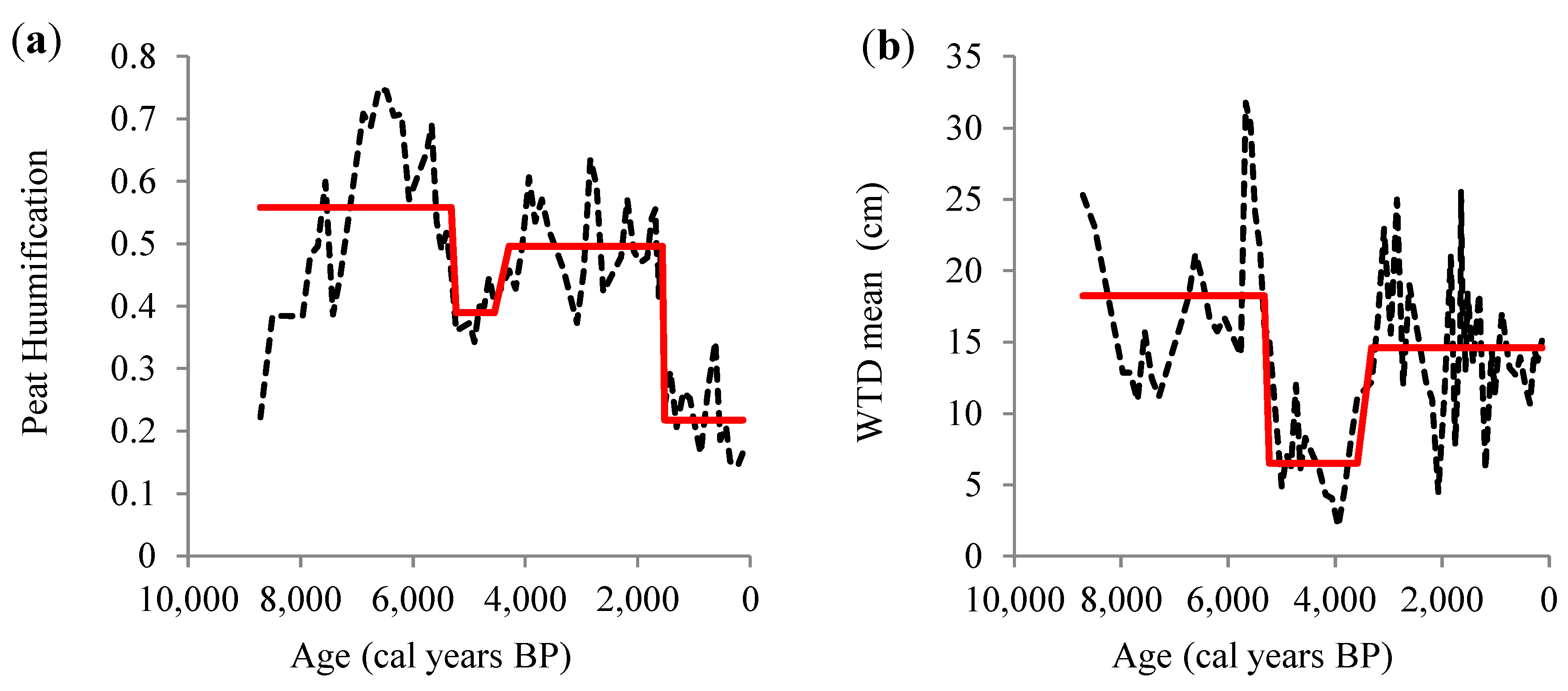
3.1.1. The Long-Term Dynamics of WTD and Peat Humification: A Step-Wise Pattern

Figure 1a illustrates the WTD values in relation to the estimated age of the deposits according to the mean depth, covering the period 8749–131 cal years BP. According to Figure 1a, there was an abrupt downward shift (occurred 5232 years BP), followed by a rapid upward shift (occurred 3316 years BP) in the WTD time-series. The statistical method used in the WDT dataset to detect the existence of these two shifts was the numerical algorithm developed by Rodionov [28]. This algorithm is based on a sequential t-test that examines the hypothesis that the average of two consecutive intervals in a time-series is significantly different [29].

Similarly, the application of the Rodionov method to the peat humification time-series (covering the common period 8749–131 cal years BP) again led to a downward shift (occurred 5232 years BP, as in the case of WTD), which followed this time by a rapid upward shift (appeared 4291 years BP) and a downward shift (occurred 1525 years BP) (see Figure 1b). The coincidence of the downward shift for the two parameters (at 5232 years BP) might indicate a specific climatic event or a physicochemical change associated with both WTD and peat humification.

Certainly, there is more to be explained about how shifts in the various series are related to each other and what they imply about Holocene climate shifts in the region. However, a clear answer to these questions requires the availability of much more data as the system under consideration is complex and complicated. However, the fact is that the present analysis shows that these two variables can change abruptly, which is similar to the behavior of the short-term climate and even the weather [30].

On small time scales, groundwater tables fall faster when peat is humified and are flashier, recovering faster after rain. In addition, during wet periods, less water is required for groundwater tables to rise in humified peatlands, which explains the faster recovery after rain and generally the more flashy behavior. Moreover, deeper groundwater tables in humified peat during dry periods lead to more severe hydrological drought than in non-humified peat [31].

On large time scales, such as those shown in Figure 1a,b, knowledge is limited. There is no doubt that the afore-mentioned finding is a result of the complex mechanisms that govern the peatlands and WTD dynamics. However, to better understand hydrological, physicochemical changes taking place as a result of WTD changes, the detailed study of the evolution of the organic matter of the bulk peat and its humified fraction is required. In this regard, it should be recalled that peatland ecosystems have been shown to be net CO₂ sinks and net greenhouse gases sources on a long-term basis. More specifically, when they are drained, the peatland areas become a threat to the environment as the thickness of the aerobic layer increases. This leads to an increase in the rate of decomposition of organic matter, and so peatlands may change from net carbon sinks to large carbon sources, resulting in increased CO₂ and CH₄ emissions from these organic soils.

All of the shifts in the regime described above reflect sudden paleoclimatic changes that may affect the parameters studied in different ways, as suggested by Payne et al. [17]. However, these rapid shifts have recently also been identified in the sea surface temperature (SST) time-series and hurricane frequency over the North Atlantic (in 1925/1926 and 1987/1988) This may indicate that there are similar natural laws and mechanisms that govern the paleo and modern climate, which could have potential effects on future climate shifts and crossing tipping points due to the well-established interactions of intrinsic climate dynamics and anthropogenic enhancement of the atmospheric greenhouse effect [32].

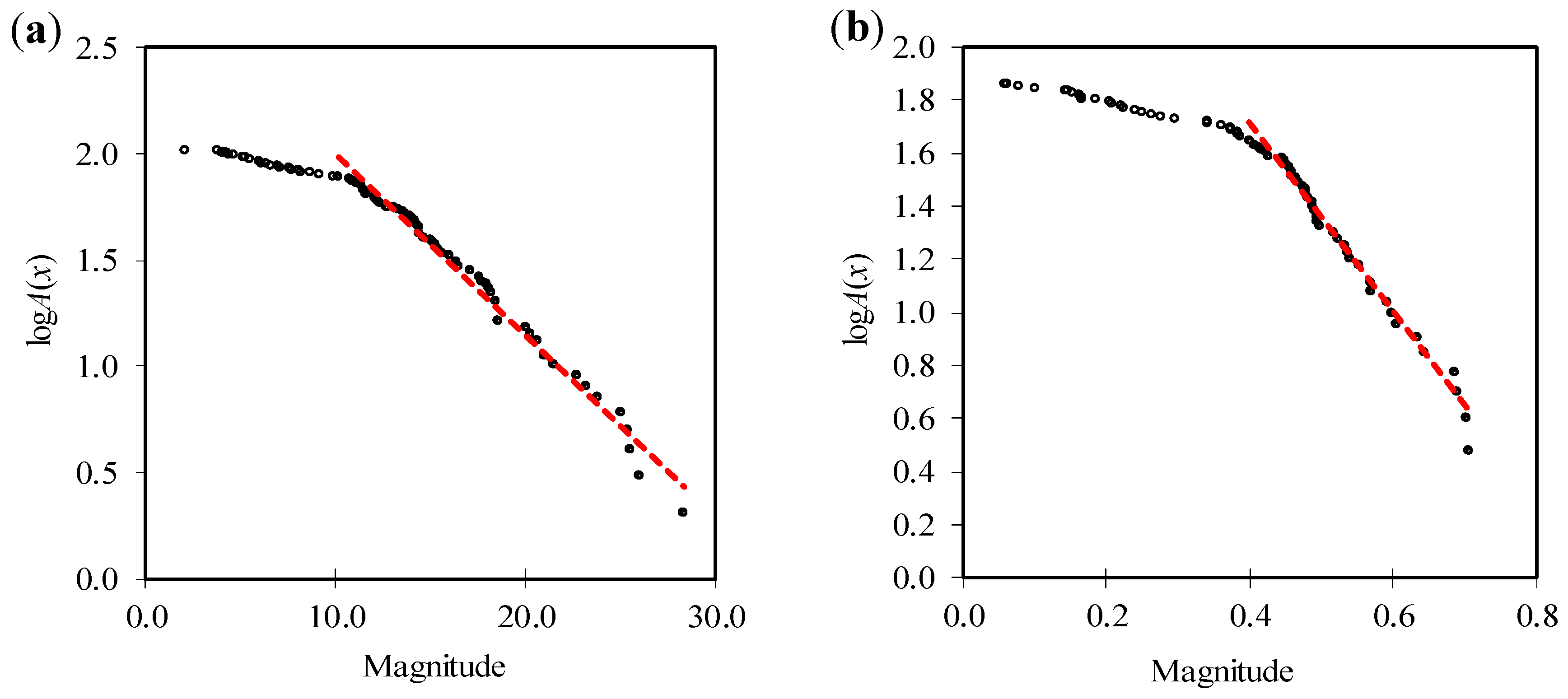
3.1.2. Gutenberg–Richter Law on WTD and Peat Humification

In the context of climate change problems, such as those mentioned in the previous section, techniques for estimating exceedance probabilities and return periods for extreme events are a matter of first priority. To that end, good, high-resolution paleoclimatic files can be quite useful in this context, as they provide opportunities for evaluating more extreme events over longer periods [32,33,34].

In this direction, the next step in our analysis was to investigate the statistical distributions of WTD and peat humification values. As it turned out, the normal distribution fits significantly to the values of both paleoclimate parameters, and this result was checked using appropriate statistical tests, such as Kolmogorov–Smirnov and Anderson–Darling tests, at a 95% confidence level. However, focusing on the high values of WTD and peat humification, we showed that they were better described by a semi-logarithmic distribution (i.e., the Gutenberg–Richter–GR law) than the Gaussian distribution.

In this regard, calculating the cumulative absolute frequency A(x) (which indicates the times that a value x is exceeded into a dataset) and plotting the logA(x) versus x (see Figure 2a,b), a statistically significant linear fit yielded (see Equation (1)). More specifically, for the high x values of WTD (or peat humification) with x ≥ x_o = 10.1 (with x ≥ x_o = 0.4) the estimated b–value was 0.085 ± 0.002 (3.55 ± 0.07) and the a–value was 2.84 ± 0.02 (3.13 ± 0.04). The x_o–values were selected to achieve the best statistical significance for the R²-coefficient of determination and the a–, b–coefficients (according to the F–test and t–test, respectively, at the 95% confidence level).

Then, we introduced in our analysis the concept of natural time (mentioned in Section 2), putting in the equation $\frac{A_h}{A_s}$ = ${10}^{b\left(X_s-X_h\right)}$ as $X_h$–value the data average μ (i.e., 13.8 and 0.42 for WTD and peat humification, respectively) and as $X_s$–value a slightly lower value than μ (i.e., 11.3 and 0.41 for WTD and peat humification, respectively).

Figure 3a,b shows $A_h$ versus $A_s$ revealing, indeed, the expected constant ratio $\frac{A_h}{A_s}$ = $c$ which verified the GR-model for the high values of both parameters. Applying the F-test (t-test), we established the linear fit $A_h$ = c∙$A_s$, in terms of the statistical significance of R² (slope c).

Finally, the introduction of the ratio $c$ (i.e., 0.66 ± 0.066 and 0.92 ± 0.043 for WTD and peat humification, respectively) and the difference $(X_s$ – $X_h$) (i.e., 2.5 and 0.01 for WTD and peat humification, respectively) into the equation $\frac{A_h}{A_s}$ = ${10}^{b\left(X_s-X_h\right)}$, provides a coefficient b’, which is approximately equal to the b–value obtained by Equation (1) for each parameter examined. Therefore, the use of the natural time concept helped our analysis to re-affirm the reliability of the GR that fits the high values of both paleoclimate parameters.

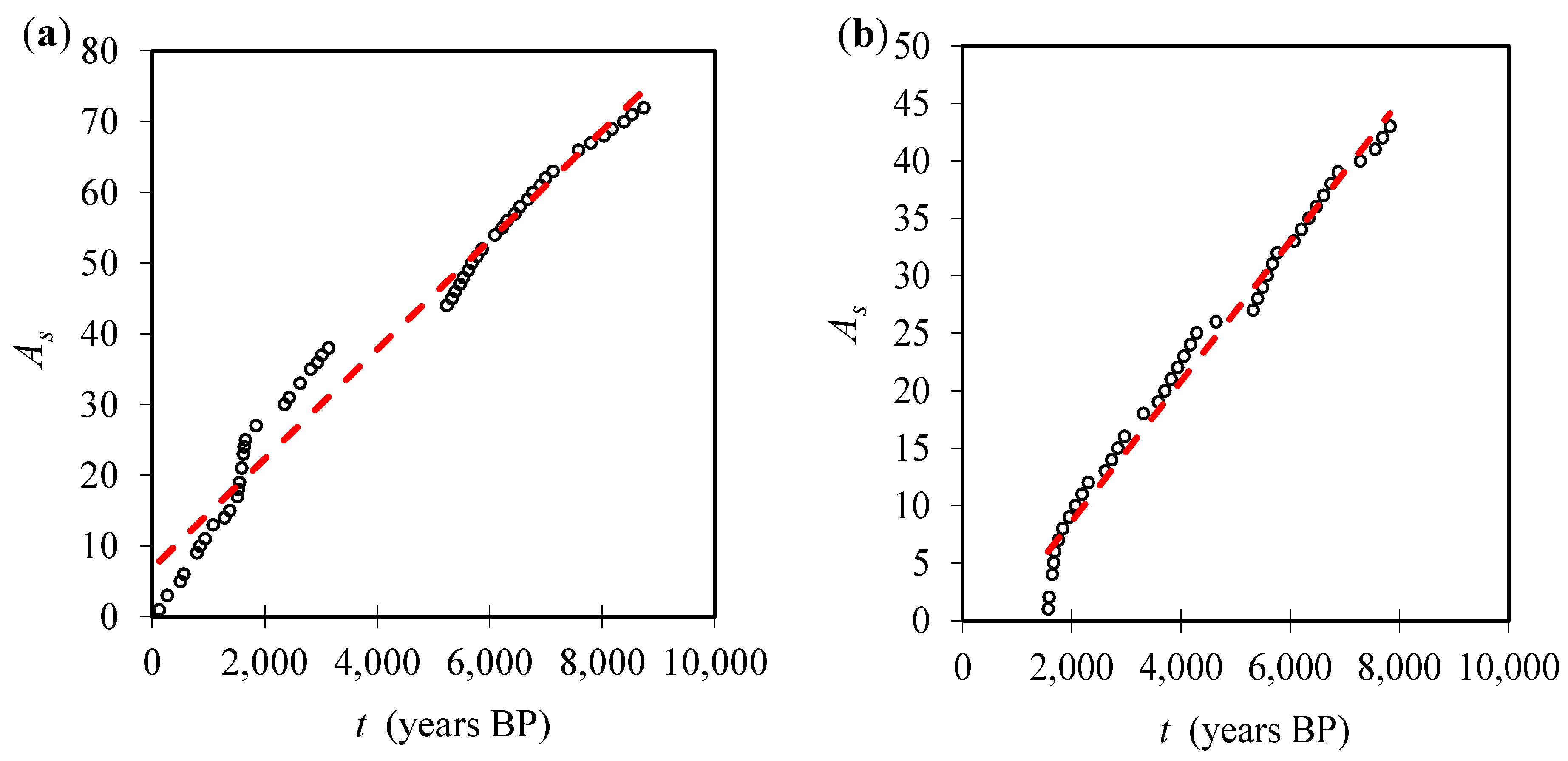
3.1.3. Occurrence Rate for High WTD and Peat Humification Values

In the following, we employed the natural time tool again to estimate the rate of occurrence for high values of WTD and peat humification. To this aim, we calculated the rate of occurrence $\frac{d{A}_s}{dt}$ (between 8749–131 cal years BP for WTD and 8714–131 cal years BP for peat humification) by determining the slope of the linear regression applied to the plot of $A_s$ as a function of the age. The linear fit in this plot was characterized by a high R²–value (which was statistically significant at 95% confidence level), indicating a constant occurrence rate for the lower values (with x > $X_s$) of the two parameters examined (see Figure 4a,b).

After that, we plotted the empirical and the nowcasted A_h–values (derived from the product of the A_s–values and the constant ratio c) versus the age, over the periods 8749–131 cal years BP (8714–131 cal years BP) for WTD (or peat humification) (see Figure 5a,b). The Wilcoxon signed-rank test confirmed the assumption that the empirical and the nowcasted A_h–values have the same distribution, at a 95% confidence level.

Then, the occurrence rate of high values with size x > $X_h$ (i.e., $\frac{d{A}_h}{dt}=\frac{d{A}_s}{dt} ·$c) showed a time interval of about 152 years and 109 years (for WTD and peat humification, respectively) between two consecutive high values.

The last step of our analysis was to estimate the time intervals between extreme events of both parameters examined. So, we calculated the average waiting time t for a specific large value (with size x) of WTD and peat humification using Equation (2), where b comes from Equation (1) and $X_s$–value was 11.3 and 0.41 for WTD and peat humification, respectively (see Figure 6a,b). For example, the average time interval for a WTD (or peat humification) value with x = 14 (x = 0.45) was estimated at approximately 169 (137) years, with confidence interval [165.2, 172.9] ([134.3, 139.8]). Thus, using Figure 6a,b as a nowcasting tool, we can predict the average waiting time for high values of both WTD and peat humification. Estimating the corresponding 1σ–error bars, the uncertainties in the waiting times seem to have a small range for both parameters [35].

3.2. Studying the CMI and Aridity Index Using the Novel Nowcasting Tool

3.2.1. Study of the Long-Term Dynamics of CMI and Aridity Index

To classify the surface moisture conditions in the next step, we analyzed the time-series of two modeled climatic indices (i.e., Climate Moisture Index (CMI) and Aridity Index) over the past 8700 cal years BP from Staroselsky Moch peatland, Russia [17]. In contrast to the long-term dynamics of WTD and peat humification, no abrupt shift of the CMI and Aridity Index time-series was found (see Figure 7a,b).

3.2.2. Gutenberg–Richter Law on CMI and the Aridity Index

The Kolmogorov–Smirnov test suggested an insufficient determination of the normal distribution for CMI and Aridity Index values at a 95% confidence level. It would be of great interest to use the natural time tool in our analysis by applying the nowcasting model described above, at high values of CMI and Aridity indices (see Figure 8a,b).

Table 1. The results of the statistical analysis of the Gutenberg–Richter (GR)-model applied (a) to the large Climate Moisture Index (CMI) values and (b) to the large Aridity Index values for the last 8700 cal years.

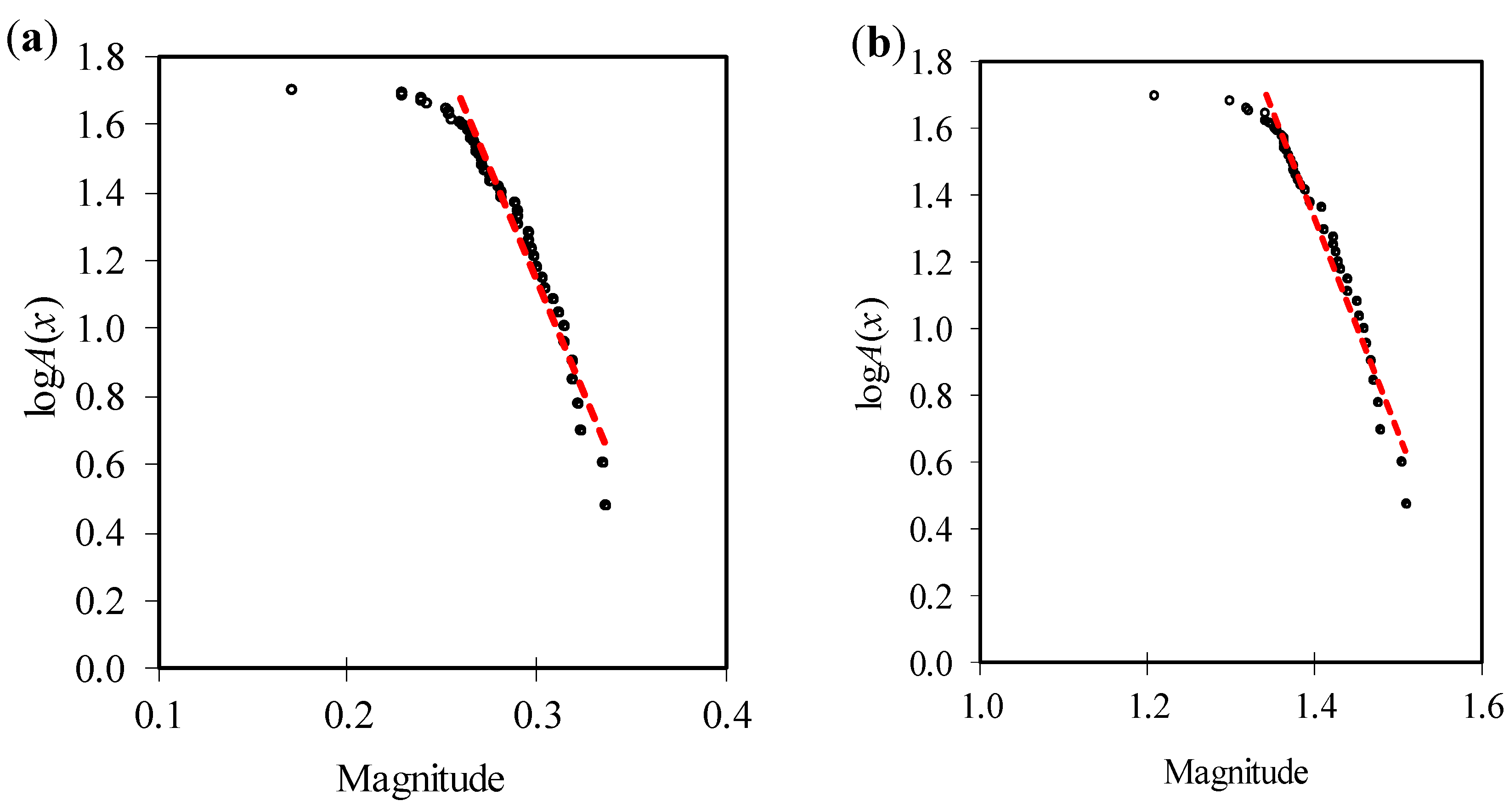
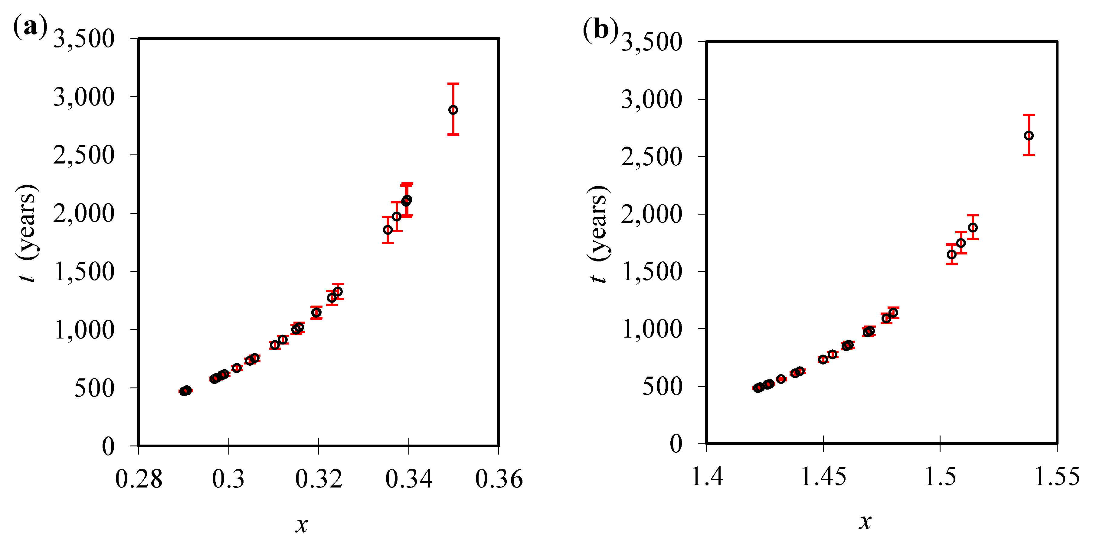
(a) Statistically Significant Semi-Logarithmic Fit to the Large CMI Values (with x ≥ 0.26):	logA(x) = a − b·x with b = 13.2 ± 0.46 and a= 5.1 ± 0.13
${\mathit{X}}_{\mathit{h}}$–value:	0.284
${\mathit{X}}_{\mathit{s}}$–value:	0.278
$\frac{{\mathit{A}}_{\mathit{h}}}{{\mathit{A}}_{\mathit{s}}}$:	constant ratio c = 0.84
b΄:	12.6 (which is very close to b)
$\frac{\mathit{d}{\mathit{A}}_{\mathit{s}}}{\mathit{d}\mathit{t}}$:	0.0031
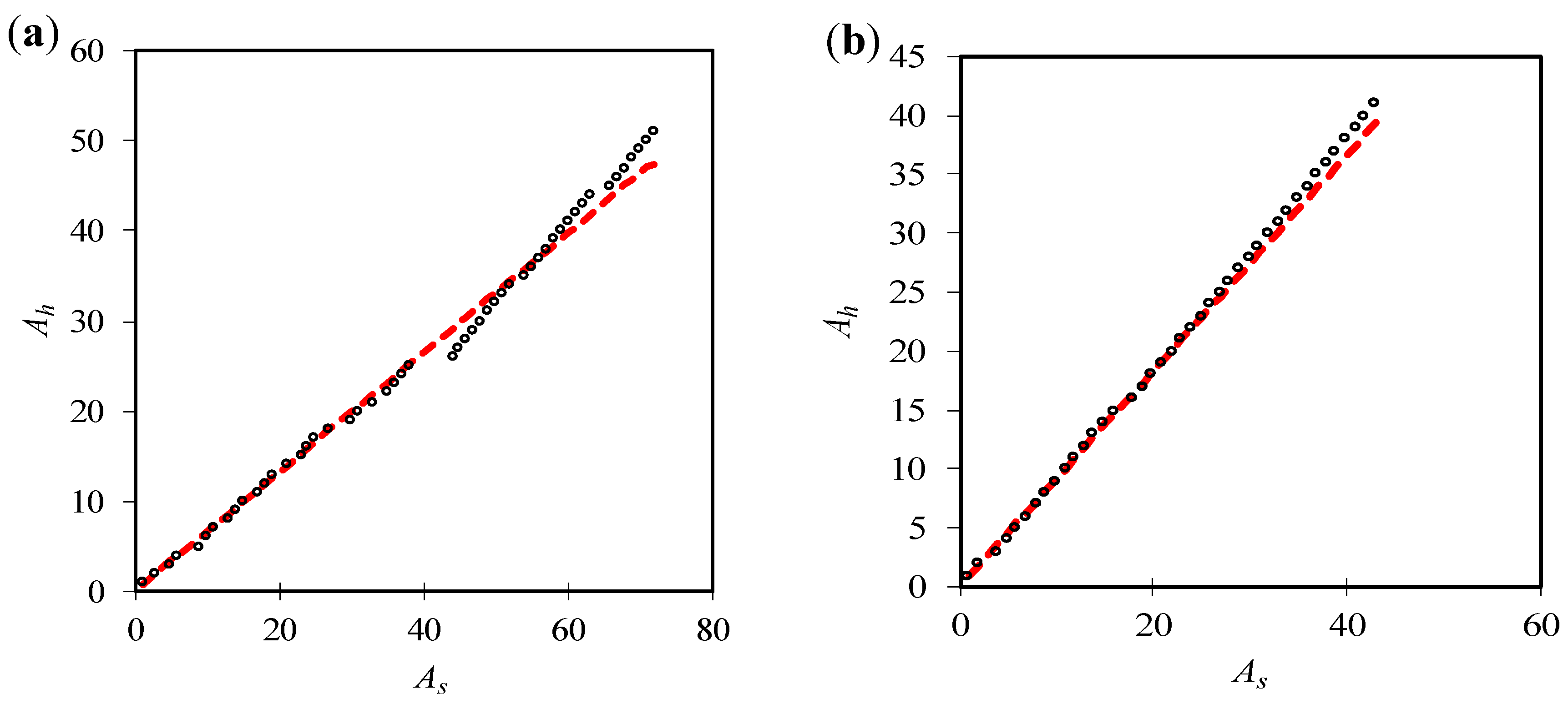
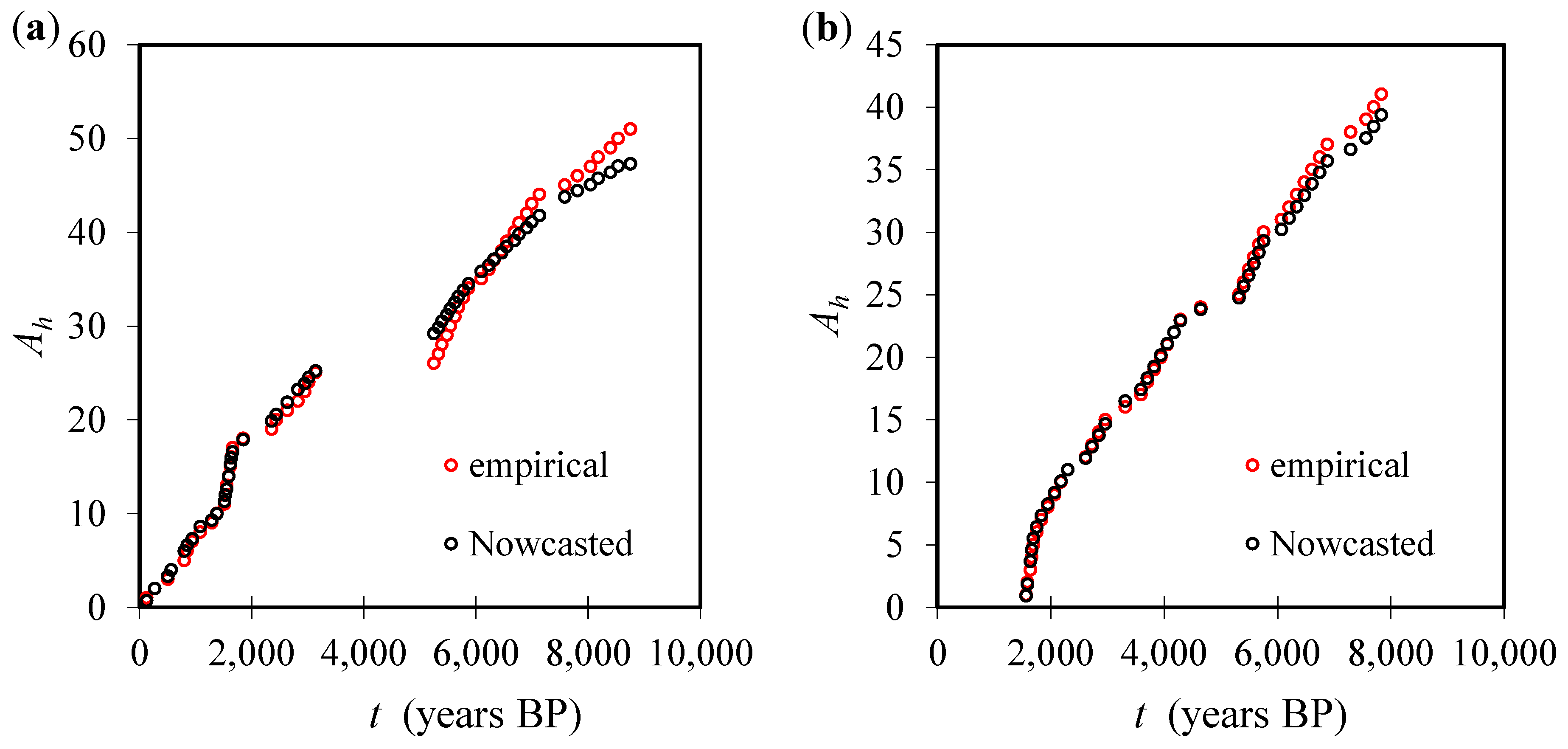
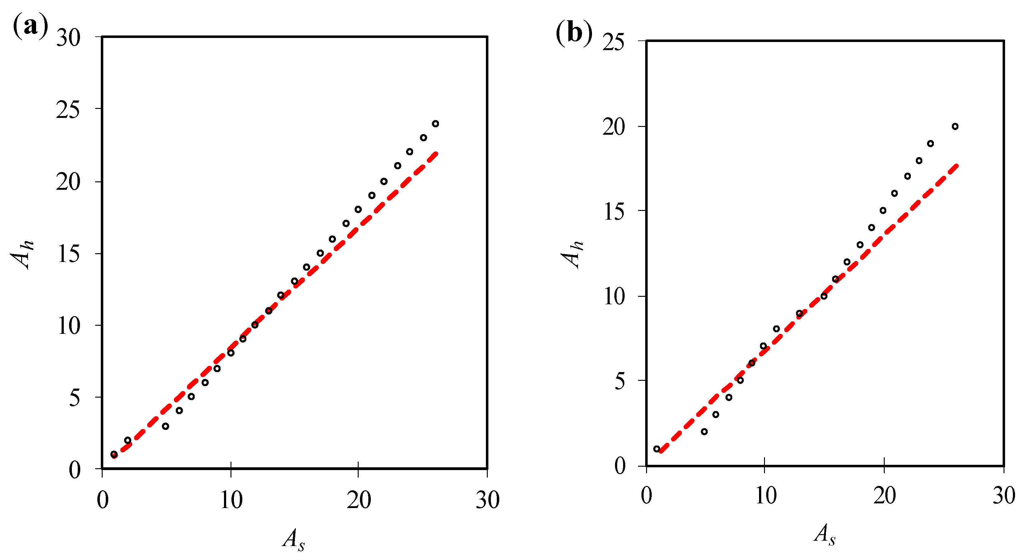
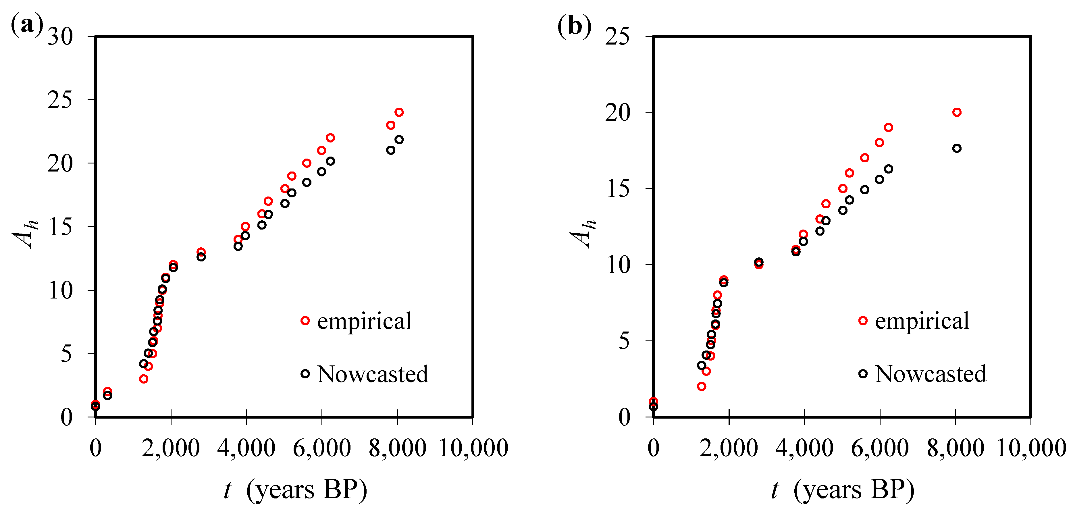
empirical vs. nowcasted Ah–values:	significant agreement, established by Wilcoxon signed-rank test
(b) Statistically Significant Semi-Logarithmic Fit to the Large Aridity Indices (with x ≥ 1.34):	logA(x) = a − b·x with b = 6.4 ± 0.19 and a = 10.3 ± 0.28
${\mathit{X}}_{\mathit{h}}$–value:	1.42
${\mathit{X}}_{\mathit{s}}$–value:	1.39
$\frac{{\mathit{A}}_{\mathit{h}}}{{\mathit{A}}_{\mathit{s}}}$:	constant ratio c = 0.68
b΄:	6.0 (which is very close to b)
$\frac{\mathit{d}{\mathit{A}}_{\mathit{s}}}{\mathit{d}\mathit{t}}$:	0.0032
empirical vs. nowcasted Ah–values:	significant agreement, established by Wilcoxon signed-rank test

a,b and Figure 8, Figure 9, Figure 10, Figure 11 and Figure 12 show the statistical results derived from the GR-model. All of these results were established using appropriate statistical tests.

The analysis and the results presented above showed that both in the conventional time scale and in the natural time domain, high values of WTD, peat moisture, CMI, and Aridity Index follow the GR law. Based on this finding and employing the natural time concept, the new nowcasting tool was developed. Next, the application of this model to three climate parameters was demonstrated. From the analysis presented and the results drawn above, it emerged that this new view of time reveals novel dynamical features hidden behind time series that describe complex systems, such as Earth’s global climate, and can be identified when the system approaches a critical point. Therefore, natural time plays a key role in predicting impending extreme events, which, according to GR law, are rare.

As can be seen above, the concept of natural time is the basis of the proposed new nowcasting tool. This tool provides the average waiting time (with satisfactory accuracy) for high values of WTD, peat moisture, CMI, and the Aridity Index, thus forecasting the behavior of the relevant climatic events in the region. For instance, peatlands store more CO₂ than forests, and, on the other hand, they maintain heavy rainfall and release the water more gradually, helping to control flooding. Therefore, the peat bog series seems to be related to CO₂ concentration and rainfall. Determining the probability of an extreme peat moisture value, we could nowcast the abrupt changes in these two climatic parameters (i.e., CO₂ and rainfall).

Thus, the proposed model is a suitable tool for the timely protection of vulnerable communities in developing countries from the effects of climate change. Its integration into development policy will substantially contribute to the synergies between mitigation and energy use by demonstrating the potential for long-term weather forecasting and climate, thus enhancing the desired mitigation, adaptation, and sustainable development.

4. Conclusions

In this study, we looked at the dynamics of time series for variables, such as water table depth (WTD) and the Climate Moisture Index (CMI). We have demonstrated that these variables may indicate abrupt or gradual changes, reminiscent of the behavior of the shorter-term climate and even weather first discovered by Edward Lorentz about 60 years ago [30]. Then we used statistical techniques (Kolmogorov–Smirnov and Gutenberg–Richter) to model WTD and CMI, respectively. We used these to estimate the time interval between maxima using a new time domain (natural time) to anticipate future climate changes.

More specifically, our analysis yielded the following main results:

(1) Sudden shifts in WTD and peat humification time-series (for the common period 8749–131 cal years BP) were detected. Although the reason is not clear, the fact is that these variables may feature abrupt or step-wise changes, which is similar to the behavior of shorter-term climate and even weather (e.g., [30,36,37]).

(2) In contrast to the long-term dynamics of WTD and peat humification, no abrupt shift in the time-series of the modeled climatic parameters, namely CMI and Aridity Index, was observed in the last 8700 cal years.

(3) Both in the conventional time scale and in the recently introduced natural time domain, the high values of WTD, peat humification, CMI, and the Aridity Index followed the GR law. Based on this finding, a novel nowcasting tool was developed that derives the mean waiting time for the high values of WTD, peat humification, CMI, and Aridity Index with satisfactory accuracy.

It is emphasized that the above-mentioned results and the novel nowcasting tool presented in this study can be used to accurately assess the deposition of airborne contaminants transported over large distances, as ombrotrophic peat bog is polluted by atmospheric deposition mechanisms [38].

In addition, the proposed algorithm integrated into the development policy aims both at the timely protection of vulnerable communities from the effects of extreme climate change phenomena and at strengthening sustainability, mitigation, and adaptation.

References

- Krapivin, V.F.; Varotsos, C.A.; Soldatov, V.Y. Simulation results from a coupled model of carbon dioxide and methane global cycles. Ecol. Mod. 2017, 359, 69–79. [Google Scholar] [CrossRef]
- Snyder, P.K.; Foley, J.A.; Delire, C. Evaluating the influence of different vegetation biomes on the global climate. Clim. Dyn. 2004, 23, 279–302. [Google Scholar] [CrossRef]
- Foley, J.A.; Levis, S.; Prentice, I.C.; Pollard, D.; Thompson, S.L. Coupling dynamic models of climate and vegetation. Glob. Chang. Biol. 1998, 4, 561–579. [Google Scholar] [CrossRef] [Green Version]
- Efstathiou, M.N.; Varotsos, C.A. On the altitude dependence of the temperature scaling behavior at the global troposphere. Int. J. Remote Sens. 2010, 31, 343–349. [Google Scholar] [CrossRef]
- Varotsos, C.A.; Mazei, Y.A. Future temperature extremes will be more harmful: A new critical factor for improved forecasts. Int. J. Environ. Res. Public Health 2019, 16, 4015. [Google Scholar] [CrossRef] [PubMed] [Green Version]
- Varotsos, C.A.; Mazei, Y.A.; Burkovsky, I.; Efstathiou, M.N.; Tzanis, C.G. Climate scaling behavior in the dynamics of the marine interstitial ciliate community. Theor. Appl. Climatol. 2016, 125, 439–447. [Google Scholar] [CrossRef]
- Varotsos, C.; Mazei, Y.; Efstathiou, M. Paleoecological and recent data show a steady temporal evolution of carbon dioxide and temperature. Atmos. Pollut. Res. 2020, 11, 714–722. [Google Scholar] [CrossRef]
- Varotsos, P.A.; Sarlis, N.V.; Tanaka, H.K.; Skordas, E.S. Some properties of the entropy in natural time. Phys. Rev. E 2005, 71, 032102. [Google Scholar] [CrossRef] [Green Version]
- Krzyszczak, J.; Baranowski, P.; Hoffmann, H.; Zubik, M.; Sławiński, C. Analysis of climate dynamics across a european transect using a multifractal method. In ITISE 2016: Advances in Time Series Analysis and Forecasting; Rojas, I., Pomares, H., Valenzuela, O., Eds.; Springer: Cham, Switzerland, 2017. [Google Scholar] [CrossRef] [Green Version]
- Rundle, J.B.; Luginbuhl, M.; Giguere, A.; Turcotte, D.L. Natural time, nowcasting and the physics of earthquakes: Estimation of seismic risk to global megacities. In Earthquakes and Multi-Hazards Around the Pacific Rim; Williams, C., Peng, Z., Zhang, Y., Fukuyama, E., Goebel, T., Yoder, M., Eds.; Birkhäuser: Basel, Switzerland, 2019; Volume 2. [Google Scholar]
- Blackford, J. Peat bogs as sources of proxy climatic data: Past approaches and future research. In Climate Change and Human Impact on the Landscape; Chambers, F.M., Ed.; Springer: Rotterdam, The Netherlands, 1993; pp. 47–56. [Google Scholar]
- Chambers, F.M.; Booth, R.K.; De Vleeschouwer, F.; Lamentowicz, M.; Le Roux, G.; Mauquoy, D.; Nichols, J.E.; van Geel, B. Development and refinement of proxy-climate indicators from peats. Quat. Int. 2012, 268, 21–33. [Google Scholar] [CrossRef] [Green Version]
- Blackford, J. Palaeoclimatic records from peat bogs. Trends Ecol. Evol. 2000, 15, 193–198. [Google Scholar] [CrossRef]
- Blundell, A.; Hughes, P.D.; Chambers, F.M. An 8000-year multi-proxy peat-based palaeoclimate record from Newfoundland: Evidence of coherent changes in bog surface wetness and ocean circulation. Holocene 2018, 28, 791–805. [Google Scholar] [CrossRef] [Green Version]
- Novenko, E.Y.; Tsyganov, A.N.; Babeshko, K.V.; Payne, R.J.; Li, J.; Mazei, Y.A.; Olchev, A.V. Climatic moisture conditions in the north-west of the mid-Russian upland during the Holocene. Geogr. Environ. Sustain. 2019, 12, 188–202. [Google Scholar] [CrossRef]
- Novenko, E.; Tsyganov, A.; Volkova, E.; Babeshko, K.; Lavrentiev, N.; Payne, R.; Yu, M. The Holocene palaeoenvironmental history of Central European Russia reconstructed from pollen, plant macrofossil and testate amoeba analyses of the Klukva peatland, Tula region. Quat. Res. 2015, 83, 459–468. [Google Scholar] [CrossRef]
- Payne, R.J.; Malysheva, E.; Tsyganov, A.; Pampura, T.; Novenko, E.; Volkova, E.; Babeshko, K.; Mazei, Y. A multi-proxy record of Holocene environmental change, peatland development and carbon accumulation from Staroselsky Moch peatland, Russia. Holocene 2015, 26, 314–326. [Google Scholar] [CrossRef]
- Turcotte, F.A. A Method for Aircraft Icing Diagnosis in Precipitation. Ph.D. Thesis, McGill University, Montreal, QC, Canada, October 1994. [Google Scholar]
- Luginbuhl, M.; Rundle, J.B.; Turcotte, D.L. Natural time and nowcasting earthquakes: Are large global earthquakes temporally clustered? In Earthquakes and Multi-Hazards Around the Pacific Rim; Williams, C., Peng, Z., Zhang, Y., Fukuyama, E., Goebel, T., Yoder, M., Eds.; Birkhäuser: Cham, Switzerland, 2019; Volume 2. [Google Scholar] [CrossRef]
- Tsyganov, A.N.; Babeshko, K.V.; Novenko, E.Y.; Malysheva, E.A.; Payne, R.J.; Mazei, Y.A. Quantitative reconstruction of peatland hydrological regime with fossil testate amoebae communities. Russ. J. Ecol. 2017, 48, 191–198. [Google Scholar] [CrossRef]
- Chambers, F.M.; Beilman, D.W.; Yu, Z. Methods for determining peat humification and for quantifying peat bulk density, organic matter and carbon content for palaeo studies of climate and peatland. Mires Peat 2010, 7, 1–10. [Google Scholar]
- Willmott, C.J.; Feddema, J.J. A more rational climatic moisture index. Prof. Geogr. 1992, 44, 84–88. [Google Scholar] [CrossRef]
- Olchev, A.; Getmanova, E.; Novenko, E. A modeling approach for reconstruction of annual land surface evapotranspiration using palaeoecological data. IOP Conf. Ser. Earth Environ. Sci. 2020, 438, 012021. [Google Scholar] [CrossRef]
- Reimer, P.J.; Bard, E.; Bayliss, A.; Beck, J.W. IntCal13 and Marine13 radiocarbon age calibration curves 0–50,000 years cal BP. Radiocarbon 2013, 55, 1869–1887. [Google Scholar] [CrossRef] [Green Version]
- Kolmogorov, A.N. Sulla determinazione empirica di una legge di distribuzione. Inst. Ital. Attuari Giorn. 1933, 4, 83–91. [Google Scholar]
- Andersson, M.E.; Verronen, P.T.; Rodger, C.J.; Clilverd, M.A.; Sepala, A. Missing driver in the Sun–Earth connection from energetic electron precipitation impacts mesospheric ozone. Nat. Commun. 2014, 5. [Google Scholar] [CrossRef] [PubMed] [Green Version]
- García-Marín, A.P.; Estévez, J.; Alcalá-Miras, J.A.; Morbidelli, R.; Flammini, A.; Ayuso-Muñoz, J.L. Multifractal analysis to study break points in temperature data sets. Chaos 2019, 29, 093116. [Google Scholar] [CrossRef] [PubMed]
- Rodionov, S.N. A sequential algorithm for testing climate regime shifts. Geophys. Res. Lett. 2004, 31. [Google Scholar] [CrossRef] [Green Version]
- Varotsos, C.A.; Efstathiou, M.N.; Christodoulakis, J. Abrupt changes in global tropospheric temperature. Atmos. Res. 2019, 217, 114–119. [Google Scholar] [CrossRef]
- Lorenz, E.N. Deterministic nonperiodic flow. J. Atmos. Sci. 1963, 20, 130–141. [Google Scholar] [CrossRef] [Green Version]
- Taufik, M.; Veldhuizen, A.A.; Wösten, J.H.M.; van Lanen, H.A.J. Exploration of the importance of physical properties of Indonesian peatlands to assess critical groundwater table depths, associated drought and fire hazard. Geoderma 2019, 347, 160–169. [Google Scholar] [CrossRef]
- Varotsos, C.A.; Franzke, C.L.E.; Efstathiou, M.N.; Degermendzhi, A.G. Evidence for two abrupt warming events of SST in the last century. Theor. Appl. Climatol. 2014, 116, 51–60. [Google Scholar] [CrossRef] [Green Version]
- Hosseini, S.R.; Scaioni, M.; Marani, M. Extreme Atlantic hurricane probability of occurrence through the metastatistical extreme value distribution. Geophys. Res. Lett. 2020, 47. [Google Scholar] [CrossRef]
- Frederikse, T.; Buchanan, M.K.; Lambert, E.; Kopp, R.E.; Oppenheimer, M.; Rasmussen, D.J.; van de Wal, R.S. Antarctic ice sheet and emission scenario controls on 21st-century extreme sea-level changes. Nat. Commun. 2020, 11, 1–11. [Google Scholar] [CrossRef] [Green Version]
- Benestad, R.E. Record-values, nonstationarity tests and extreme value distributions. Glob. Planet. Chang. 2004, 44, 11–26. [Google Scholar] [CrossRef]
- Lovejoy, S.; Varotsos, C. Scaling regimes and linear/nonlinear responses of last millennium climate to volcanic and solar forcings. Earth Syst. Dyn. 2016, 7, 133–150. [Google Scholar] [CrossRef] [Green Version]
- Varotsos, C.A.; Efstathiou, M.N.; Cracknell, A.P. Sharp rise in hurricane and cyclone count during the last century. Theor. Appl. Climatol. 2015, 119, 629–638. [Google Scholar] [CrossRef]
- Miszczak, E.; Stefaniak, S.; Michczyński, A.; Steinnes, E.; Twardowska, I. A novel approach to peatlands as archives of total cumulative spatial pollution loads from atmospheric deposition of airborne elements complementary to EMEP data: Priority pollutants (Pb, Cd, Hg). Sci. Total Environ. 2020, 705, 135776. [Google Scholar] [CrossRef] [PubMed]