


Introduction
The release of elastic (seismic) energy within a glacier or ice sheet indicates a response to dynamic forcing or transient change in motion (see reviews by Podolskiy and Walter, Reference Podolskiy and Walter2016; Aster and Winberry, Reference Aster and Winberry2017). Glaciological processes such as brittle fracture (e.g. Neave and Savage, Reference Neave and Savage1970; Mikesell and others, Reference Mikesell2012), hydraulic resonance in moulins (e.g. Roeoesli and others, Reference Roeoesli, Walter, Ampuero and Kissling2016) and changes in the basal hydraulic system (e.g. Walter and others, Reference Walter, Dalban Canassy, Husen and Clinton2013; Vore and others, Reference Vore, Bartholomaus, Winberry, Walter and Amundson2019) produce signals that can be detected in seismic records. Furthermore, changes in seismic characteristics over time can indicate temporally gradual changes in a glacial system that are not as readily apparent through other observations.
Seismic sources located on and near glaciers and ice sheets often show diurnal or seasonal patterns in activity (e.g. MacAyeal and others, Reference MacAyeal2018; Podolskiy and others, Reference Podolskiy, Fujita, Sunako, Tsushima and Kayastha2018; Zhang and others, Reference Zhang2019). This activity, referred to as seismicity, comprises a superposition of discrete, transient seismic events over a background of persistent, low-amplitude microseismic energy that evolves with time. The variability of such seismicity tends to match the variability of environmental processes that include summertime melting and runoff at the glacier surface (Hart and others, Reference Hart2019); englacial and subglacial water flow (Röösli and others, Reference Röösli2014); snow redistribution (Allstadt and Malone, Reference Allstadt and Malone2014; Chaput and others, Reference Chaput2018); fluctuations in air temperature (Podolskiy and others, Reference Podolskiy, Fujita, Sunako, Tsushima and Kayastha2018); and thermal bending and fracture of ice during melt/freeze cycles on supraglacial ponds (MacAyeal and others, Reference MacAyeal2018), sea ice (Bažant, Reference Bažant1992) and lake ice (Ghofrani and Atkinson, Reference Ghofrani and Atkinson2018; Kavanaugh and others, Reference Kavanaugh2019). In this paper, we use the term ‘environmental microseismicity’ to refer to the background component of periglacial and glacial seismicity (i.e. low-amplitude, temporally variable microseismicity described above), distinct from the discrete, transient seismic events.
Many passive glacial seismology experiments focus on transient seismic waveforms generated by discrete, glaciogenic events. We emphasize herein that the geophysical ‘interest’ of a seismic signal (transient or environmental) depends on the particular problem under study. This reflects the philosophy that ‘one person's signal is another's noise’ (e.g. Stein and Wysession, Reference Stein and Wysession2003, p. 141). Cryoseismology analogously requires analysis methods that identify signals both in pursuit of or in spite of temporally variable environmental microseismicity. Researchers therefore remain challenged to understand how environmental microseismicity (including glaciogenic microseismicity) interacts with other glaciogenic signals.
Environmental microseismicity presents a particular challenge to seismic waveform detection: patterns in both environmental microseismicity and discrete icequakes can vary over matching timescales (e.g. diurnal or seasonal). The signal-to-noise ratio (SNR) for a seismic waveform (‘signal’) with a given amplitude will change depending on temporally variable background levels of microseismic energy (‘noise’). A digital signal detection algorithm may or may not identify a waveform of a given amplitude depending on the noise conditions (as described in glacial environments by Walter and others, Reference Walter, Deichmann and Funk2008; Dalban Canassy and others, Reference Dalban Canassy, Faillettaz, Walter and Huss2012). This implies that choosing one detection method over another during a seismic experiment can influence an observer's interpretation of temporal patterns of seismic activity.
Locally-deployed passive seismic networks provide a monitoring technology that can capture small-magnitude seismic sources. For example, MacAyeal and others (Reference MacAyeal2018) used local records to show that event frequency of diurnally variable and thermally activated fracture sources on an ice-shelf are well described by a Gutenberg–Richter type law. This law predicts that the number of small-magnitude icequakes is orders of magnitude greater than the number of large-magnitude icequakes. However, sensors can only record these small sources above noise at local distances. To better interpret such geophysically interesting, small-magnitude seismic sources, researchers should first assess how their observation is biased by temporally variable environmental microseismicity and detector design choices.
In this paper, we compare the detection capability of two automatic seismic event detectors (named ‘2dof’ and ‘3dof’) under varying environmental microseismicity conditions. The two degree of freedom (2dof) detector implements the same algorithm as the noise-adaptive detector of Carmichael and others (Reference Carmichael2015). The three degree of freedom (3dof) is another noise-adaptive detector; it implements different parameter estimators and includes a third degree of freedom to account for correlation in the environmental microseismicity. This modification is inspired by an infrasound event detector developed by Arrowsmith and others (Reference Arrowsmith2015); their detector included a third degree of freedom so as to ‘reduce false detections associated with coherent continuous-wave sources such as microbaroms or wind farms’ (p. 1412).
We observe temporally variable inter-detector differences in event counts and ability to detect small events. We attribute these detection differences to differences in how the detectors interpret environmental microseismicity. To directly test the ability of both detectors to identify waveforms over a range of magnitudes, we perform a waveform infusion experiment and describe how these results can inform our interpretations of measured seismicity. We further relate our detector's capabilities to physical dimensions of glaciogenic seismic sources (i.e. surface crack dimensions).
Our study uses data from Taylor Glacier, Antarctica; however, the detection methods we discuss are applicable to all glacier settings. Geophysical interpretation of Taylor Glacier's seismic response to forcings (including brine release, meltwater generation and katabatic winds) is beyond the scope of this paper. Therefore, we do not locate sources of discrete icequakes or compare our measurements of seismicity against energy balance or thermal bending models as done elsewhere (e.g. Carmichael and others, Reference Carmichael, Pettit, Hoffman, Fountain and Hallet2012; MacAyeal and others, Reference MacAyeal2018). Throughout the paper, we use the term ‘icequake’ if the likely source is on the glacier or the more general terms ‘events’ and ‘waveforms’ if no specific glacial source is implied.
Analyzing seismic data collected from glaciers
Waveform detection operations that process large sets of seismic data (e.g. this study, 14 months of data from three stations with sample rates of 200 s$^ {-1}$ ) require automated processing techniques. The most general digital waveform detection method (requiring the least prior knowledge of waveform shape) is the short-term average to long-term average (STA/LTA) detector (Earle and Shearer, Reference Earle and Shearer1994; Withers and others, Reference Withers1998; Song and others, Reference Song, Warpinski, Toksöz and Kuleli2014). Algorithms implementing these detectors operate from a binary hypotheses test on the recorded data: either a seismogram contains just noise or it contains a signal contaminated with noise. To evaluate which hypothesis is true, the STA/LTA algorithm compares an STA estimate of data energy (variance) to an LTA estimate of data energy. When this ratio exceeds a prescribed threshold value, the STA/LTA algorithm triggers, or declares a waveform detection.
For any detector, the false-alarm rate quantitatively estimates how often the detector triggers on background noise when no waveform is present. Similarly, the detection capability qualitatively describes how well the detector successfully identifies events. For two detectors with the same false-alarm rate, the detector that identifies waveforms with a smaller SNR more often has a higher detection capability. Furthermore, the same waveform detector can have variable detection capability under variable noise conditions.
Most STA/LTA detectors used to process seismic data collected from glacial environments compare the STA/LTA statistic against a constant threshold value that thus defines the lowest energy signal the detector can register (e.g. Walter and others, Reference Walter, Deichmann and Funk2008; Carmichael and others, Reference Carmichael, Pettit, Hoffman, Fountain and Hallet2012; Dalban Canassy and others, Reference Dalban Canassy, Faillettaz, Walter and Huss2012; Röösli and others, Reference Röösli2014). The STA/LTA statistic is a proxy for a waveform's SNR. Thus, a constant threshold value precludes detection of small amplitude waveforms during high-noise conditions that would otherwise be detected under low-noise conditions, resulting in a temporal variability in detector capability. For instance, Walter and others (Reference Walter, Deichmann and Funk2008) attribute variability in their STA/LTA detector capability to a diurnal surface melt cycle. Dalban Canassy and others (Reference Dalban Canassy, Faillettaz, Walter and Huss2012) similarly describe a correlation between STA/LTA detection capability and modeled glacier runoff over day- to week-periods. Therefore, temporal variability in waveform detection capability has the potential to bias an observer's interpretation of the temporal variability in icequake activity (Röösli and others, Reference Röösli2014; Carmichael, Reference Carmichael2019).
One particular strategy developed to account for temporally variable detection capability implements a two-stage process. First, a constant threshold value determines a set of events. Second, a time series of these identified events is analyzed with respect to event size. If the time series reveals a temporally variable absence of small events, a secondary threshold is established above these smallest event sizes. A second pass retains only events that are sufficiently energetic to exceed the secondary detection floor (Walter and others, Reference Walter, Deichmann and Funk2008, Fig. 5). Above this detection floor, detector capability is considered to be temporally constant (Walter and others, Reference Walter, Deichmann and Funk2008; Dalban Canassy and others, Reference Dalban Canassy, Faillettaz, Walter and Huss2012; Röösli and others, Reference Röösli2014). That is, researchers assume that events above the secondary threshold are correctly identified regardless of variable background noise. The drawback to this approach is that the small events detected during low-noise conditions are discarded during the secondary thresholding step, thereby complicating the study of processes that generate these low-energy signals.
Another version of the STA/LTA event detector is the noise-adaptive STA/LTA detector. Using this event detection strategy, the detector sets a temporally variable threshold that adapts to the current noise conditions (Carmichael and others, Reference Carmichael2015). This method effectively adjusts the threshold value by monitoring changes in the statistical distribution of the STA/LTA time series. These detectors maintain a constant (estimated) false-alarm rate by setting variable thresholds; in contrast, constant threshold STA/LTA detectors have a variable false-alarm rate.
In this paper, we evaluate two distinct, noise-adaptive STA/LTA seismic event detectors using data collected from Taylor Glacier. Both detectors impose a constant false-alarm rate and calculate noise-adaptive thresholds over 15-min time windows.
Study site and observation network
Taylor Glacier flows from Taylor Dome on the East Antarctic ice sheet and terminates in Taylor Valley 100 km downstream. Near the terminus, deformation is characterized by plug-like flow of clean cold ice over a layer of more rapidly deforming debris-rich basal ice (Pettit and others, Reference Pettit, Whorton, Waddington and Sletten2014). Ice cliffs (20–30 m high) form the margin of the glacier in the terminus region. The central portion of the glacier terminates into the ice-covered west lobe of Lake Bonney, while the remainder of the glacier terminates onto land. Near the terminus, deep seasonally-occupied supraglacial meltwater channels (Johnston and others, Reference Johnston, Fountain and Nylen2005) generate substantial across-flow changes in ice thickness (Badgeley and others, Reference Badgeley2017). Subglacially-sourced, iron-rich, hypersaline brine flows episodically via a surface crevasse near the terminus; the resulting feature is called Blood Falls (Mikucki and others, Reference Mikucki, Foreman, Sattler, Berry Lyons and Priscu2004).
In a prior seismic experiment implementing a constant-threshold STA/LTA detector for Taylor Glacier data, Carmichael and others (Reference Carmichael, Pettit, Hoffman, Fountain and Hallet2012) observe diurnal patterns in seismicity during periods when there is no surface melt predicted by a calibrated surface energy balance model (model is described in Hoffman and others, Reference Hoffman, Fountain and Liston2008). By locating these microseismic events, Carmichael and others (Reference Carmichael, Pettit, Hoffman, Fountain and Hallet2012) find sources in both the lake ice and glacier ice. In contrast, during periods of surface melt, the diurnal seismicity signal is suppressed. Instead, larger repeating icequakes consistent with volumetric source mechanisms (crack opening) dominate the seismic record.
The glacial and periglacial environments of and around Taylor Glacier host many processes that we expect to generate larger seismic events as well as variable levels of environmental microseismicity. These include: ice-cliff calving and collapse, seasonal melt and associated runoff in supraglacial channels, episodic release of subglacial brine through a crevasse (Blood Falls release), thermally-driven fracture of lake or glacier ice, meltwater-driven fracture, avalanching at nearby glaciers and crevassing within the glacier ice.
To monitor such sources of seismicity at Taylor Glacier, we deployed a sub-network of three seismometers (Sercel L-22 geophones) that operated from December 2013 through January 2015. We installed one geophone (JESS) on the glacier near an ice cliff and two into the frozen sediment to the north (KRIS) and south (CECE) of the terminus (Fig. 1). Quanterra Q330 digitizers sampled our geophone data at 200 s$^{ - 1}$ . The seismic data described in this study are available for public access through the IRIS Data Management Center (Pettit, Reference Pettit2013).

Fig. 1. Study location at the terminus of Taylor Glacier with land-based seismometers CECE and KRIS and on-ice seismometer JESS. Base image: Google, Maxar Technologies, image date: 5 December 2008. Antarctica outline from Quantarctica.
Despite the high latitude of the field area, which is typically associated with 24-h daylight in the summer, the steep topography bounding the glacial valley imposes a diurnal pattern on solar insolation with the sun dropping below the mountains in the evenings. We therefore use solar noon as a reference local time, in addition to UTC time, when presenting our results. For this location, solar noon is closest to UTC + 11 (note that this is not the same as the local McMurdo time zone). During the winter, the sun remains below the horizon, however we maintain the same ‘local solar noon time’ offset of UTC + 11 for consistency.
Methods
We organize this section as follows: we introduce the statistical distribution (F-distribution) of the STA/LTA detection statistic under a hypothesis testing framework, describe the two seismic event detectors, conduct a semi-empirical experiment to evaluate detector performance and compute empirical performance curves, and relate detection capability to source size. Table 1 provides a complete list of abbreviations and mathematical symbols.
Table 1. Symbols and descriptions

Units given where applicable in square brackets; physical variables refer to the cylindrical coordinate system. In this table and elsewhere, we adopt the following conventions: mathematical symbols (except for probabilities) are italicized while abbreviations are not; vectors, matrices and tensors are in boldface and symbols with hats designate estimated values.
F-distributions, null and alternative hypotheses
We implement two distinct STA/LTA seismic energy detectors that use noise-adaptive thresholds to identify waveforms. Both the 2dof and 3dof detectors calculate the STA/LTA statistic from two, quasi-independent estimates of sample variance at each time index in a seismogram data stream where such ratios are well defined, and use this statistic to measure signal strength. The STA/LTA statistic follows a so-called F-distribution when the samples drawn from the seismogram data are themselves described by Gaussian statistics (Kay, Reference Kay1998). Each detector fits probability density function (PDF) curves to the histogram of the F-distributed STA/LTA statistic by estimating PDF parameters that best fit these data. The parameter set estimate that best fits the STA/LTA statistic (‘fit parameters’) describe the shape of theoretical predicted F-PDF curves. When the detector processes a data stream of zero-mean, partially white noise, probability theory predicts that these fit parameters describe an STA/LTA statistic with a density that has a central F-PDF curve shape. In contrast, when data include nonzero-mean signals that superimpose with this noise, theory predicts that the fit parameters describe an STA/LTA statistic with a non-central F-PDF curve shape (Kay, Reference Kay1998). We assume that the data are dominated by noise (the signal sparsity assumption) so we fit the STA/LTA statistic computed from our seismic data with central F-PDF curves. Under this assumption, the middle 95% of a histogram formed from an STA/LTA statistic is well-described by a central F-distribution; we do not fit the smallest or largest 2.5% of the STA/LTA statistic.
The two detectors we compare differ in the number of degrees of freedom used to parameterize the F-PDF curves. The 3dof detector estimates three parameters which determine the shape of the F-PDF, while the 2dof detector estimates only two parameters.
We use the STA/LTA statistic to evaluate two hypotheses, namely, that a short-term sample of the data represents only noise (zero mean) or that the short-term sample contains noise plus discrete event (e.g. icequake) signals (nonzero mean). Thus, we can state our hypotheses as ${\cal H}_0$ : the STA/LTA statistic follows a central F-distribution if there is no signal, vs ${\cal H}_1$
 : the STA/LTA statistic follows a non-central F-distribution if a signal is present (Blandford, Reference Blandford1974). We assume the central distribution (${\cal H}_0$
 ) when we determine the threshold that is based on the middle 95% of the histogram. Our algorithm tests the STA/LTA values (not just the middle 95%) against this threshold to detect waveforms. If any STA/LTA values are declared as ‘events’ above the threshold, theory predicts that the resulting F-PDF distribution containing all STA/LTA values should instead form a non-central F-PDF distribution (${\cal H}_1$
 ). To the extent that the null hypothesis provides a good data model, our prescribed, predicted false-alarm rate approximately confines the actual false-detection rate (i.e. the rate of false-positive event declarations). We discuss the predicted false-alarm probability in subsection ‘Invert F-CDF to find threshold value’.
Detector descriptions
The general workflow for processing 15-min subsets of data proceeds in six stages for both detectors. We (1) prepare (preprocess) the data, (2) calculate the STA/LTA statistic time series, (3) search for best fit parameter sets using multiple parameter estimators and initializations to minimize the fit error between the data (normalized STA/LTA histograms) and the theoretical F-PDF curve, (4) select the theoretical F-PDF with the lowest fit error among the best parameter sets returned by the previous step, (5) invert the associated central F-cumulative distribution function (CDF) to find the threshold value associated with a desired false-detection probability ${\rm Pr}_{FA}^{{\rm Pre}}$ and (6) identify events from short-term windows with STA/LTA values above this threshold. The two different detectors implement distinct parameter estimators; one detector allows for a third degree of freedom parameter to account for data correlation between the short- and long-term windows and the other does not. We describe individual processing steps below.
Preprocess data
We first subtract any linear trend from each time series with the MATLAB function detrend.m that implements least-squares regression. We then remove spectral content outside the frequency range [2.5,35] Hz with a 4th-order minimum phase Butterworth filter designed to retain signal causality and mitigate distortion of the original waveform. We use a minimum phase filter because we plan to use this dataset in the future to identify source locations and we want to preserve arrival times. We choose this frequency range based on visual inspection of spectrograms in which we observe broadband events with apparent diurnal (summertime) and multi-day (wintertime) trends in activity. In the subsequent empirical performance quantification, we detrended, tapered, zero-padded and then filtered the waveform data.
Calculate STA/LTA statistic
The STA/LTA statistic z i(x) at time sample i of digitized, multichannel seismogram data x is the ratio of two statistically independent estimates of data variance $\hat{\sigma }_i^2$ . An STA/LTA algorithm computes the numerator (STA) from N 1 consecutive samples starting with sample i and the denominator (LTA) from N 2 consecutive samples preceding sample i:

where time t = t S corresponds to index i that separates the neighboring short-term sample from the long-term sample, and $x_k^2 = x_{EHE\comma k}^2 + x_{EHN\comma k}^2 + x_{EHZ\comma k}^2$ is sample energy of x at sample k, measured in counts. We notationally distinguish parameters that we estimate from data like sample variance with hats (e.g. $\hat{\sigma }^2$
 ) to distinguish them from their true values (σ 2).
The STA/LTA algorithms calculate ratios z i(x):

for each sample i such that N 2 + 2 ⩽ i ⩽ N (15) − N 1, where N (15) is the number of data samples in the 15-min subset of the data record. We calculate the data histogram comprising z i(x) using the centered 95% quantile ${\rm Hist}\lpar z\rpar \vert _{2.5}^{97.5}$ that counts data over evenly spaced bins equal in number to the square root of the sample count within each 95% quantile. In other words, we use the middle 95% of the STA/LTA ratios calculated from Eqn (2) over the 15 min (N (15)) subset of the data stream to generate the data histogram.
Search for multiple parameter set estimates using different parameter estimators/initializations
We fit F-PDF curves to the normalized histograms of the STA/LTA statistic output by each detector by selecting PDF parameters that minimize mismatch between the data histogram and theoretical PDF curve. Specifically, these curve-fitting strategies minimize the L2 norm of the difference between the normalized data histogram ${\rm Hist}\lpar z\rpar \vert _{2.5}^{97.5}$ and the theoretical PDF, $f_Z\lpar z\semicolon \;{\cal H}_0\rpar$
 . Manual experiments indicated that using the middle 95% provided a good compromise between including sufficient data and excluding outliers. Both detector algorithms implement the MATLAB function fminsearch.m to find parameters that minimize these norms. When fitting the F-PDF curves, we assume the null hypothesis, which posits that the 15-min data window does not contain a seismic signal – that is, ${\rm Hist}\lpar z\rpar \vert _{2.5}^{97.5}$
 follows a density described by a central F-PDF.
The 3dof detector estimates three parameters which determine the shape of the F-PDF. Two of the three parameters, N E1 and N E2, define the effective number of statistically independent samples within the short- and long-term windows. For instance, within each window, we generally expect that samples that are close in time to each other will be more correlated than samples that are farther apart. The third parameter is c, which represents the statistical dependence of the estimated data variability between the short- and long-term windows. Two of the parameter estimators in the 3dof detector allow the third degree of freedom parameter c to vary freely, while the other two estimators impose constraints on c. Appendix A contains complete descriptions of the four parameter estimators.
The 2dof detector is only parameterized by N E1 and N E2. The 2dof detector constrains the parameter c = 1 such that the algorithm assumes that the short- and long-term data variance are effectively independent. Appendix A provides complete descriptions of the three initializations implemented by the 2dof detector.
We emphasize that N E1, N E2 and c are unknown; therefore, our detector algorithms estimate these scalars from the data. The 3dof detector implements four different F-PDF parameter estimators, and returns four sets of best estimates: $\lsqb \hat{N}_{E1}\comma \;\hat{N}_{E2}\comma \;\hat{N}_{E2}/\hat{N}_{E1}\rsqb _{P1}$ , $\lsqb \hat{N}_{E1}\comma \;\hat{N}_{E2}\comma \;1\rsqb _{P2}$
 , $\lsqb \hat{N}_{E1}\comma \;\hat{N}_{E2}\comma \;\hat{c}\rsqb _{P3}$
 and $\lsqb \hat{N}_{E1}\comma \;\hat{N}_{E2}\comma \;\hat{c}\rsqb _{P4}$
 . The 2dof detector initializes one F-PDF parameter estimator with three separate initial parameterizations, and returns three sets of best estimates: $\lsqb \hat{N}_{E1}\comma \;\hat{N}_{E2}\rsqb ^{\rm {\prime}}$
 , $\lsqb \hat{N}_{E1}\comma \;\hat{N}_{E2}\rsqb ^{\rm \prime\prime }$
 and $\lsqb \hat{N}_{E1}\comma \;\hat{N}_{E2}\rsqb ^{\rm {\prime}\prime\prime }$
 . Subscripts (e.g. P1) notationally designate parameter set estimates resulting from different parameter estimators and primes (′, ′′, ′′′) designate parameter set estimates resulting from different initializations of the same parameter estimator.
Select theoretical F-PDF with the lowest fit error from results of all parameter estimators/initializations
We next calculate the fit error associated with the best parameter set estimates returned by each fit estimator (3dof case: four sets of estimates) or initialization (2dof case: three sets of estimates). As an example, we calculate the fit error for the third parameter set estimate for the 3dof detector by substituting $\lsqb {{\hat{N}}_{E1}\comma \;{\hat{N}}_{E2}\comma \;\hat{c}} \rsqb _{P3}$ into the norm functional:

where the form of the equation is similar to that of Eqn (A5) and z 1 = (N 1/N 2) z. We calculate e 3dof, P1, e 3dof, P2, and e 3dof, P4 analogously. We select the smallest of the four fit errors and return the associated parameter triplet as the best parameter set estimate for the 3 dof detector.
Our process is similar for the 2dof detector. For example, we substitute the parameter output sets from the three initializations into the error equation corresponding to Eqn (A1) to estimate $e_{{\rm 2dof}}^{'}$ as:
as:

The 2dof algorithm selects the parameter set associated with the minimum fit error among all initialization schemes.
Invert F-CDF to find threshold value
We parameterize the inverse F-CDF with the best estimates from the previous step to determine a threshold value consistent with the desired predicted false-alarm probability. If the 3dof best parameter set corresponded to P1 or P3, the scaled version of the STA/LTA statistic z 1 replaces z (Eqns A3 and A5). We scale the STA/LTA statistic for the 3dof detector by the third degree of freedom $\hat{c}$ in all cases.
To establish event detection thresholds, we use a fixed, predicted false-alarm probability ${\rm Pr}_{FA}^{{\rm Pre}}$ of 10−7 false alarms per window (short-term plus long-term window duration = 3.28 s) that equates to ~1 predicted false alarm per year (Slinkard and others, Reference Slinkard2014, p. 2774). We note that increasing the predicted false-alarm probability will increase the number of detected events. However, our goal is not to detect the maximum number of events but rather to investigate how incorporating temporal correlation into our degrees of freedom (2dof vs 3dof) impacts event detection within the same false-alarm rate bounds. Our choice of 10−7 false alarms per window is typical of other waveform detection applications (e.g. Slinkard and others, Reference Slinkard2014). We then implement MATLAB function finv.m to compute a detector threshold η as estimate $\hat{\eta }$
 that is consistent with the desired ${\rm Pr}_{FA}^{{\rm Pre}}$
 (Kay, Reference Kay1998). Using the 2dof detector case as an example, the $\hat{\eta }$
 value that establishes this ${\rm Pr}_{FA}^{{\rm Pre}}$
 under ${\cal H}_0$
 is:
is:

where $F_Z\lpar {z\semicolon \;{\cal H}_0} \rpar$ is the CDF corresponding to PDF $f_Z\lpar {z\semicolon \;{\cal H}_0} \rpar$
 , and $F_Z^{{-}1} \lpar {{\rm Pr}\semicolon \;{\cal H}_0} \rpar$
 is the inverse CDF evaluated at Pr. We emphasize that η is estimable as $\hat{\eta }$
 from Eqn (5) and imperfectly known, as with $\hat{N}_{E1}\comma \;\hat{N}_{E2}$
 and $\hat{c}$
 . We then assign our resultant $\hat{\eta }$
 values to compute the predicted probability ${\rm Pr}_D^{{\rm Pre}}$
 that the detector correctly identifies a seismic signal buried in the noise under ${\cal H}_1$
 :
:

where the CDF $F_Z\lpar z\comma \;{\cal H}_1\rpar$ is a non-central F-distribution function with parameters $\hat{N}_{E1}$
 and $\hat{N}_{E2}$
 degrees of freedom, and non-centrality parameter λ. This scalar λ implicitly parameterizes Eqn (6) and is directly proportional to the SNR of a waveform that is included in the shorter window of the STA/LTA detector (Eqn B2). Graphically, λ quantifies the separation between the ${\cal H}_0$
 and ${\cal H}_1$
 PDF curves. A larger λ value (relative to zero) indicates a greater separation between these curves; it therefore indicates more confidence in ${\cal H}_1$
 . A smaller λ value indicates less confidence (weaker SNR and less probable waveform detections). When λ = 0 no separation between the ${\cal H}_0$
 and ${\cal H}_1$
 PDF curves exists. Because λ depends on both waveform and microseismicity characteristics, we cannot predict it in advance of data collection. We relate λ to physical dimensions of glaciogenic seismic sources in a subsequent section. Appendix B more completely describes the λ estimator.
Identify events from short-term windows above threshold
The final step in event identification is to search through the data stream and identify short-term windows with STA/LTA values above the threshold $\hat{\eta }$ determined in the previous step. Our STA/LTA detector algorithms require processing parameters to uniquely assign detection times and statistics to isolated waveforms. For instance, when our detectors process a particular icequake waveform, they often produce STA/LTA statistics that exceed the threshold estimate $\hat{\eta }$
 over the entire duration of that icequake's waveform. To avoid redundant detection at multiple sample points on this waveform, our detectors define the peak value within any collection of consecutive samples exceeding the threshold as the detection statistic for the underlying signal, and the associated time as the event time. Both detectors output a file for each day which includes detection results, fit parameters and other file attributes. The net result is a time series of identified events; we show an example time series in Figure 2.

Fig. 2. Example summary output of the 3dof detector that processed data recorded by JESS on 21 May 2014 10.02.35 UTC. (a) Seismograms of pre-processed three channel data (EHE, EHN and EHZ). (b) Time series of STA/LTA statistic (see Eqns 1 and 2) superimposed with a threshold for event detection consistent with a ${\rm Pr}_{FA}^{{\rm Pre}} = 10^{{-}7}$ false-alarm rate; red circles mark when this statistic exceeds the threshold (dashed horizontal line). Shaded vertical regions indicate waveforms; the central waveform with the largest detection statistic corresponds to the template implemented in infusion experiments. (c) Normalized data histogram (bars) of the STA/LTA statistic superimposed with the best-fit central F-PDF (curve); the dashed vertical threshold line corresponds to the dashed horizontal threshold shown in the STA/LTA plot at left. The norm of the difference between the histogram and PDF curve at right (the bars and solid curve) defines our estimate of e 3dof (initialization subscript suppressed). We show 3 min of data for visual clarity in preference to the 15 min data windows that we use in all processing routines described elsewhere in this paper.
Semi-empirical performance comparison
We run a semi-empirical experiment to quantify how well the 3dof and 2dof detectors count icequakes under real noise conditions. Our original data streams contain unknown numbers of ‘real’ events. We therefore create a hybrid data stream comprising the original geophone data and a known number of infused, amplitude-scaled icequake waveforms. We emphasize that this infusion routine is distinct from the convolution routines used to generate synthetic seismograms. Our infusion routine linearly adds the amplitude-scaled icequake waveforms to the original, unscaled data stream in the time domain (see Carmichael and Nemzek, Reference Carmichael and Nemzek2019 for further details).
We run both detectors on the hybrid data stream and count the number of infused waveforms that our detectors find over a range of scaled amplitudes that we relate to pseudo-magnitude, after Carmichael and Nemzek (Reference Carmichael and Nemzek2019). The template icequake waveform that we scale for our infusion process (Fig. 2a, prominent waveform near 90 s) has amplitude A 0 and corresponds to an unknown reference magnitude m 0. We premultiply this template waveform by a scalar A j related to icequake magnitude: $A_j = 10^{m_j-m_0}A_0$ where m j is the relative magnitude (‘pseudo-magnitude’) of the hypothetical icequake source that excites a scaled waveform of amplitude A j. We index magnitude and amplitude by j to indicate that we sample relative magnitude over a uniform 200 point grid, and limit its domain to: −2.5⩽m j − m 0⩽0 because this range yielded meaningful empirical performance curves (see ‘Results’ section). We create this hybrid data stream using 900-s (15-min) windows, and infuse 28 identical copies of the scaled waveform evenly over time within each window.
After we infuse the scaled events, both detectors scan the entire 15-min window for events. We then check the detection results at the known infusion times to determine if the detector correctly identified the added events. Our algorithms define such detections as ‘true’ if they declare an event within N 1 samples (corresponding to 0.625 s) of the manual waveform infusion time. We repeat this detection operation for every 15-min window of the selected days and for all j scaling factors in our test domain. As we are interested in temporal differences in detection capability at diurnal and seasonal scales, we select three consecutive typical summer days and three consecutive typical winter day as test periods for the empirical performance comparison. We select these ‘typical days’ from a visual inspection of the pattern of event counts throughout the day (gray boxes highlight these days in Fig. S1). This manual review showed that these three winter and summer days represented the average (mean) pattern for their associated season well.
Empirical performance curves
We estimate the mean observed (empirical) probability $\overline {{\rm Pr}} _D^{{\rm Obs}}$ that our STA/LTA detectors identify scaled, infused waveforms by averaging the number of these same waveforms that we detect within our hybrid data produced by a hypothetical source of magnitude m j − m 0. We compute uncertainty weighted estimates as:

where the term C D is the integer number of detected events (C D ∈ [0, 28]), C T is the total number of infused waveforms (C T = 28) and e k is the window-specific fit error, for instance e 3dof (Eqn 3) or e 2dof (Eqn 4). In detail, the term $\overline {{\rm Pr}} _D^{{\rm Obs}} \lpar m_j\semicolon \;k\rpar$ refers to the count-normalized number of infused waveforms that an STA/LTA detector identifies in a 900 s window that contains a total of 28 infused waveforms, and k indexes the number of infusion routines that we apply to a 24 h dataset (1⩽k⩽96 reflects one infusion routine per 900 s).
The term $\overline {{\rm Pr}} _D^{{\rm Obs}} \lpar m_j\semicolon \;k\rpar$ therefore measures the average empirical probability that an STA/LTA detector identifies a waveform produced by a hypothetical icequake source of magnitude m j − m 0. Each subsequent down-scaling (different m j) reduces the SNR of the infused waveforms and the probability that either detector could distinguish these waveforms in the pulse train from noise. We use analogous equations for all other error-weighted results reported in this paper and omit writing the error-weighted version of each equation. Additional quantitative details of the error weighting scheme are well documented in Carmichael and Nemzek (Reference Carmichael and Nemzek2019).
The resultant locus of all points described by Eqn (7) (all j) compares STA/LTA detection rates against relative source size over our limited magnitude grid −2.5⩽m j − m 0⩽0. We calculate weighted and unweighted versions and plot these in the ‘Results’ section. Equation (7) with e k = 1 for all k defines the unweighted, mean empirical probability. To compare the spread of detection probability at different relative magnitudes, we calculate and plot the quantiles of C D/C T.
Relationship between detection capability and source size
While our semi-empirical analysis compares icequake detection rates against a measure of source size (magnitude), this analysis does not relate these magnitudes to any observable of a typical glaciogenic source. We therefore transform our magnitude grid m j − m 0 to a representative, seismogenic ice crack model to improve our understanding of the physical limits that bound our ability to detect transient icequakes in real noise. This comparison will allow us to report detection values against the spatial scale of an equivalent surface crack, even when we detect waveforms that originate from sources that are not surface cracks. We do not include complicating effects of firn or depth-dependent density changes that would complicate our model. Our objective is to bound the behavior of source effects on the non-centrality parameter λ rather than model the wavefield. Furthermore, both the source and receiver in our model are located on-ice in the ablation zone (no firn present).
We first compute the theoretical, azimuthal-integrated Rayleigh wave seismogram energy that we measure from a hypothetical, opening crack in the ice. We then compare this model against observed, integrated seismogram energy that relates to non-centrality parameter λ and measures our predicted detection probability ${\rm Pr}_D^{{\rm Pre}} \lpar {m-m_0} \rpar$ (magnitude grid index k omitted).
To construct the seismogram model, we assume that a source consists of an opening tensile crack with a crack plane perpendicular to the ice surface. We consider small cracks that radiate high frequency Rayleigh waves near the limit of our reliable detection ability, so that their wavelengths do not sample the ice (or bed) at depth well and we can therefore model the glacier ice as a half space. Under these assumptions, the frequency domain displacement at receiver location ξ created by the displacement at shallow crack source with location ξ0 has a particularly simple form: ${\bi u = }{\cal R}\lpar \varphi \rpar {\bi g}\lpar {\bi \xi }\comma \;\omega \rpar$ , where ${\cal R}\lpar \varphi \rpar$
 is the radiation pattern that varies with azimuth φ between the source and receiver, and where g(ξ, ω) is a vector independent of φ (Aki and Richards, Reference Aki and Richards2002, p. 328). This vector g(ξ, ω) depends on components of the source moment tensor M (Eqn C2), which represents the body-force equivalent of the crack face opening displacement as a weighted set of force couples, localized at source point ξ0. The analytical expressions for both ${\cal R}\lpar \varphi \rpar$
 and g(ξ, ω) appear in Appendix C where we compute the energy explicitly; we simply summarize those results here. First, we square and average this displacement ‖u(ξ, ω)‖2 over azimuth to obtain the average Rayleigh wave energy E R:

The integrated, squared radiation pattern is a function of frequency, elastic constants, crack area A, and the crack face-opening distance $\lsqb \kern-0.15em\lsqb {u\lpar {\bi \xi }\,_0\comma \;t_0\rpar } \rsqb \kern-0.15em\rsqb$ . Our notation means that the crack is located at point ξ0 and opens a distance $\lsqb \kern-0.15em\lsqb u \rsqb \kern-0.15em\rsqb$
 at time t 0. We emphasize that the energy integral refers to ice displacement in the frequency domain (Hz) and factor the crack's spatial dependence and frequency dependence into the product $\lsqb \kern-0.15em\lsqb {u\lpar {\bi \xi }_0\comma \;t_0\rpar } \rsqb \kern-0.15em\rsqb = \lsqb \kern-0.15em\lsqb {u\lpar {\bi \xi }_0\rpar } \rsqb \kern-0.15em\rsqb s\lpar \omega \rpar$
 , where s(ω) is the Fourier transform of the displacement source–time function of the crack that opens at time t 0; Appendix C documents our choice for s(ω). We then explicitly write the dependence of the integrated Rayleigh wave energy in terms of energy created in opening the crack:

where ρ is the ice density, β is the s-wave velocity in ice and the term O.T. stands for ‘other terms’ that are functions of frequency ω, density, body wave speeds and Rayleigh wave speeds. We further include physical effects of anelasticity that dispersively attenuate waveforms as they propagate from source point ξ0 to receiver point ξ (Carmichael and others, Reference Carmichael2015, Fig. 4a). To quantify such attenuation, we multiply the right-hand side of Eqn (9) by $\exp \left({{{-\omega \vert \vert {\bi \xi }-{\bi \xi }_0\vert \vert } \over {Qc_R}}} \right)$ , where Q is the surface wave quality factor and c R is the Rayleigh wave speed; we note that the phase function of the attenuation is zero in the energy function. We integrate (smooth) the result over the range of our bandpass-filtered frequencies, ω min to ω max:

where we have lumped the attenuation factor with ‘other terms’ that we integrate to define I(ω min, ω max). Importantly, Eqn (10) illustrates that azimuthally averaged Rayleigh wave energy is proportional to a transient increase in crack volume.
We relate the non-centrality term λ of the STA/LTA detector statistic to the integrated Rayleigh wave energy through Parseval's theorem. In plain words, this theorem states that the time domain energy of a signal equates to the frequency domain energy of that same signal (Stein and Wysession, Reference Stein and Wysession2003, p. 375). The ratio of this integrated signal energy to noise variance defines λ:

Equation (11) is combined with Eqn (6) to quantify the predicted probability ${\rm Pr}_D^{{\rm Pre}}$ that the STA/LTA detector will trigger on a waveform radiated by a crack of area A that opens a distance $\lsqb \kern-0.15em\lsqb {u\lpar {\bi \xi }_0\rpar } \rsqb \kern-0.15em\rsqb$
 . We note that the newly created crack volume $A\lsqb \kern-0.15em\lsqb {u\lpar {\bi \xi }_0\rpar } \rsqb \kern-0.15em\rsqb$
 relates to a length scale d as $d\lpar {A\lsqb \kern-0.15em\lsqb {u\lpar {\bi \xi }_0\rpar } \rsqb \kern-0.15em\rsqb } \rpar ^{1/3}$
 . This relationship is useful to compare detectable crack dimensions to other characteristic glaciological length scales, like thermal penetration depth of diurnal heat input. We restrict the analysis to an on-ice source and receiver. For a more complex analysis to model a receiver on a different substrate, the right-hand side of Eqn (11) would effectively be multiplied by a transmission coefficient.
Results
To explore the capabilities of these detectors and understand their differences, we focus first on an overview of the seasonally-variable seismicity characteristics as measured by the two detectors. Then we conduct a more detailed assessment of detector capabilities using results from the infusion experiment. This assessment uses data from 3-d time periods in summer and winter and relates the detection capabilities to equivalent surface crack source sizes.
Measured seismicity time series during 2014
The 2dof and 3dof detectors both measure time series that show substantial seasonal differences in seismicity (we define seismicity quantitatively as discrete seismic events per time period; here we use 15 min). Figure 3 shows seismicity for CECE, one of the land-based stations. Diurnal variability in seismicity dominates during summer months (i.e. November–January, Fig. 3, see also Figs S1a, c); in contrast, multi-day increases and decreases dominate during the winter months (i.e. April–July, Fig. 3). Furthermore, the wintertime shows consistently higher average event counts at the land-based stations.

Fig. 3. Seismic events per 15 min during 2014 at land-based station CECE as identified by the 2dof (thicker red line) and 3dof (thinner blue line) detectors. Data are smoothed with a 9-point, 2-h moving window with uniform weighting (e.g. the value for events per 15 min at 02.00 is smoothed using event counts per 15 min from the nine points: 01.00, 01.15,…, 02.45, 03.00).
The 2dof and 3dof detector results are more similar in the winter and diverge in the summer, when the 2dof detector identifies more events. Results from the other two stations show similar summertime diurnal and wintertime multi-day patterns; except that the on-ice station JESS shows a smaller inter-detector difference (Fig. S2).
Based on this initial observation of seasonally-contrasting seismicity patterns, we split our results into summer and winter cases in the following sections, using data from December 2013–January 2014 for summer cases and May 2014 for winter cases.
Measured seismicity characteristics during summer and winter
The difference between detectors with respect to the seasonal pattern in seismicity is shown in more detail in Figure 4. Here we plot the following time-averaged results from one summer month and one winter month: event counts for each detector (Figs 4a–d), inter-detector difference in event counts (Figs 4e, f) and 3dof detector $\hat{c}$ values (Figs 4g, h).

Fig. 4. (a, b) Error-weighted mean number of detected events per 15 min using the 2dof detector and (c, d) 3dof detector; (e, f) point-wise difference in error-weighted mean events between 3dof and 2dof detectors (negative numbers indicate fewer 3dof event counts relative to 2dof counts) and (g, h) error-weighted 3dof $\hat{c}$ (note: the 2dof detector has no analogous $\hat{c}$
 value). The left column is one summer month, December 2013; the right column is one winter month, May 2014. Event counts and $\hat{c}$
 values are error-weighted and time-averaged similar to Eqn (7) and binned by 15-min windows. Local solar noon time is labeled in all plots, with UTC time (bold) labeled in (g, h) only.
We observe distinct diurnal patterns during the summer in measured seismicity at all three stations. Seismicity gradually increases throughout the local evening (after ~06.00 UTC), peaks in local early morning (~16.00 UTC) and declines rapidly thereafter (Figs 4a, c). In contrast, there is no persistent diurnal seismicity pattern during the wintertime (Figs 4b, d). Seismicity measurements from on-ice station JESS show both the highest mean seismicity over the summer and the highest variability when compared to the seismicity measured on land-based stations CECE and KRIS, regardless of detector (Figs 4a, c). The inter-detector difference in measured seismicity is generally larger (more negative) in the summer at the land-based stations than at on-ice station JESS (Fig. 4e); in the winter the inter-detector difference is more similar between the stations (Fig. 4f).
The inter-detector difference is also characterized by a diurnal cycle in the summer (Fig. 4e) that is absent in the winter (Fig. 4f). The 2dof detector identifies more events per 15 min than the 3dof detector, but the inter-detector difference is largest during the high-seismicity, local morning (UTC afternoon) in the summer. The largest difference in measured seismicity also coincides with the largest values of the error-weighted third degree of freedom parameter $\hat{c}$ (Fig. 4g) that qualitatively measures higher temporal correlation in the seismic data (higher inter-sample correlation). The 3dof estimates of $\hat{c}$
 generally agree during the wintertime across the stations and over time of day (Fig. 4h).
Infusion experiment: empirical performance curves
Our waveform infusion experiment was designed to measure detector capability over a range of magnitudes. Figure 5 shows the seasonal, sub-daily and inter-station differences in event counts as a function of infused event magnitude. In the subsequent discussion, we use the phrase ‘reliably detect’ to indicate $\overline {{\rm Pr}} ^{{\rm Obs}}{\rm \ge }0.8$ , which is equivalent to the zone above the horizontal dashed line in each panel of Figure 5. We define the mean 80% detection magnitude as the minimum magnitude within our search grid at which we achieve an 80% or greater detection rate ($\overline {{\rm Pr}} ^{{\rm Obs}}{\rm \ge }0.8$
 , Table 2). Throughout the remainder of the paper, we use the terminology ‘detection magnitude’ and ‘detection capability’ somewhat interchangeably. In detail, the 80% detection magnitude is a quantitative measure based on waveform detection rates, and detector capability is a qualitative description. Smaller (more negative) 80% detection magnitudes correspond to better/stronger detection capability and larger (less negative or closer to zero) 80% detection magnitudes indicate worse/weaker detection capability.
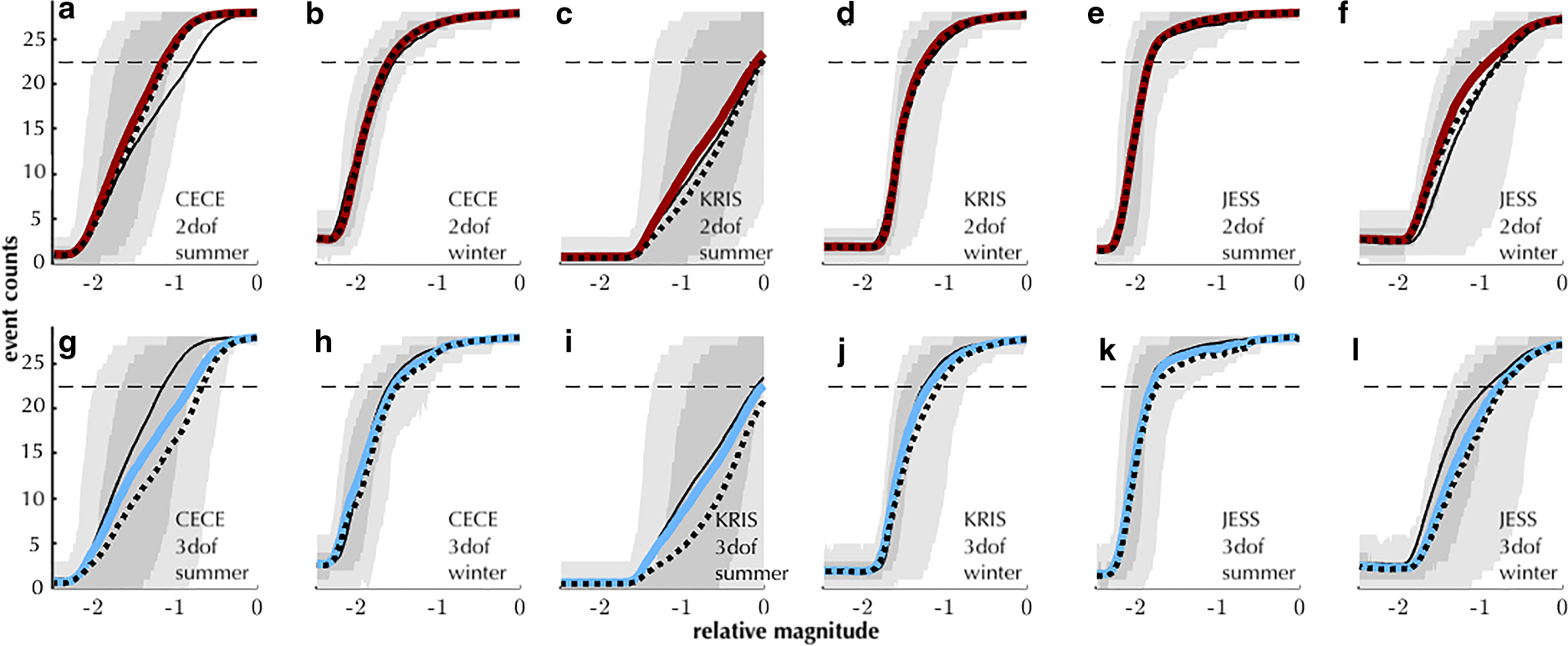
Fig. 5. Empirical performance curves for stations CECE (left block of four panels), KRIS (central block) and JESS (right block): number of detections of infused waveforms (maximum count = 28) per 15 min over the experimental range of relative magnitudes. (a–f) 2dof detector unweighted mean (bold red curves) and uncertainty-weighted mean (dotted lines). (g–l) 3dof detector unweighted mean (bold blue curves) and uncertainty-weighted mean (dotted lines). The unweighted means are the time-averaged number of events detected at each relative source size, where we average over the 3-d period. The uncertainty-weighted means account for uncertainty in the null (${\cal H}_0$ ) PDF as in Eqn (7). Within each four-panel station block, the left column shows results from three summer days (21–23 January 2014) and the right column shows results from three winter days (20–22 May 2014). In each panel, the thicker, red or blue line corresponds to the labeled detector (a–f: 2dof, g–l: 3dof) and the thinner black line is the unweighted mean from the opposite detector for comparison (a–f: 3dof, g–l: 2dof). The darker gray shading encloses the 25–75% quantile of number of detections, and the lighter shading encloses the 5–95% quantile. The horizontal dashed line in each panel is 80% of total number of infused events.
Table 2. Mean 80% detection magnitudes in pseudo-magnitude units, averaged over the 3-d test periods in summer and winter

This is the first grid value at which a 0.8 detection rate is exceeded.
The sub-daily temporal variability in detection rates across the tested magnitude range differs greatly between the summertime and wintertime records. At the land-based stations (CECE and KRIS), both the spread and the mean 80% detection magnitude are larger in the summer than the winter. At the on-ice station (JESS), the opposite is true; the spread and mean are larger in the winter (Table 2, Fig. 5). Stated differently, at the land-based stations we detect fewer discrete waveforms of low magnitude in the summer than in the winter, and their detection rates depend more on time of day.
For instance, at station CECE the 2dof detector can only reliably detect a waveform 1.15 pseudo-magnitude units below that of the template icequake waveform in the summer noise and environmental microseismicity conditions. In the winter, the same 2dof detector can reliably detect this icequake waveform 1.6 pseudo-magnitude units below that of the template waveform (Figs 5a, b, Table 2). The uncertainty in the summer detection rate estimate is also highly asymmetric (red curve not centered in the shaded quantile region). That is, the 2dof detector triggers on discrete icequakes that are a full 2.0 pseudo-magnitude units below that of the template waveform about as often as the detector triggers on events that are 1.0 pseudo-magnitude units below that of the template waveform magnitude.
The summer 3dof results from CECE and summer 2dof and 3dof results from KRIS are similarly skewed with the mean 80% detection magnitude located far to the right (larger relative magnitude) within the shaded quantile region along the 80% detection line. In other words, during some parts of the day at the land-based stations, the smallest reliably detected events are an order of magnitude smaller than the overall mean daily value for reliable detection. In contrast, icequake detection rates during the winter have comparatively low variability, lower 80% threshold mean values, and the means are more centered within the 80% detection magnitude range at the land-based stations.
Both detectors at on-ice station JESS reach 80% detection for smaller relative magnitude waveforms during the summer than in the winter (Table 2). That is, smaller icequakes are detected more frequently, and with more consistency throughout the day, in the summer at JESS than in the winter. Qualitatively, the summer curves for station JESS resemble the winter curves for the land-based stations. The mean 80% detection magnitude during the summer at JESS is smaller than at the land-based stations, but during the winter, the mean 80% detection magnitude at JESS is larger than at the land-based stations (Table 2).
Uncertainty-weighting the mean has the largest impact at the land-based stations in the summertime, particularly for the 3dof detector (thick blue vs dashed lines, Figs 5g, i). We observe the largest inter-detector differences during the summer at the land-based stations and in the winter at the on-ice station (thin black lines vs thick blue or red lines on the same subplot, Fig. 5). The range of threshold magnitudes tends to be larger for the 3dof results than for the 2dof results for a given station/season pair. This indicates greater sub-daily variability in the 3dof detector capability than in the 2dof detector capability. At the lowest detection rates (corresponding to detection pseudo-magnitudes ~−2 for station CECE and −1.5 for station KRIS in the summer for instance), the curves for the two detectors converge.
We note that for all curves, with the exception of the KRIS summer curves, plateaus in event counts at the upper and lower limits of the tested pseudo-magnitude range indicate that the range spans the transition from few, if any, event detections until event size is large enough that all events are detected. In the case of the KRIS summer curves, larger (positive) pseudo-magnitudes could be tested to reveal the upper plateau in detected event counts, but we do not extend the analysis further at this time.
Infusion experiment threshold magnitudes and measured seismicity
We compare the infusion experiment magnitude thresholds (during which we controlled the number of possible ‘true’ detections and their pseudo-magnitudes) to the event counts from the seismic data record (number of ‘true’ events and magnitudes unknown) in Figure 6. Based on the 3-d record of threshold magnitudes generated by the infusion experiment, we observe that magnitude thresholds and event counts do not consistently increase or decrease together.

Fig. 6. Relative magnitude of infused events with 80% detection (red and blue curves, left vertical axes) and measured event counts (gray and black curves, right vertical axes) during three summer (21–23 January 2014) and three winter days (20–22 May 2014) for land-based stations CECE (a, b) and KRIS (c, d) and on-ice station JESS (e, f). The thicker red curves are the 2dof detector 80% detection magnitudes, the thinner blue curves are the 3dof detector 80% detection magnitudes. Gaps in the curves indicate 15-min windows during which the detector failed to identify 80% of the infused events at any magnitude within the tested range. On the left vertical axes, larger negative numbers (further from zero) correspond to smaller magnitudes, associated with better detection capability. The gray (2dof) and black (3dof) curves are event counts from the seismicity time series obtained by processing the original data stream (not the infusion experiment). Notations 1–4 and * to *** are explained in the text. Local solar noon time is labeled in all plots, with UTC time (bold) labeled in (e, f) only. The left vertical axes are expanded for plotting purposes, note the tested range for the 80% detection magnitude is [−2.5, 0] pseudo-magnitude units.
We highlight four different relationships between detection thresholds and event counts in Figures 6c, e; both subplots are results from the summertime. In the first case, event counts increase as 80% magnitude thresholds increase (‘1’ in Fig. 6c). In the second case, event counts decrease as 80% magnitude thresholds decrease (‘2’ in Fig. 6c). In the third case, event counts increase while 80% threshold magnitude thresholds decrease (‘3’ in Fig. 6c). In the fourth case, event counts decrease while 80% magnitude thresholds increase (‘4’ in Fig. 6e).
During the 3-d time period in winter in which we performed the icequake infusion experiment, we observe a station-wide drop in detector capability from 03.30–13.30 UTC on 22 May 2014 (broad peak in 80% detection thresholds labeled ‘***’ in Figs 6b, d, f). This contrasts with some of the drops in detection capability observed in the summer, which do not always correlate network-wide. For instance, the highest peak in 80% threshold magnitude at station JESS coincides with a trough in 80% detection magnitude at station CECE (single ‘*’ labels in Figs 6a, e).
The 80% detection magnitude is generally larger and more variable during the summer than the winter at the land-based stations (Figs 6a, c vs Figs 6b, d). At station KRIS in particular, during the 3-d testing period in the summer there are 75, 15-min windows for the 2dof detector and 70, 15-min windows for the 3dof detector during which the detector does not achieve 80% detection at any magnitude in our test range. We note that while we do not know the 80% detection magnitude during these time frames, we do have a minimum bound which is the magnitude of the infused event. At station CECE, there is one 15-min window during which the 3dof detector did not achieve reliable detection. During the summer at KRIS, 80% detection magnitudes for the 2dof and 3dof detectors are similar (Fig. 6c). However, at CECE, the 2dof and 3dof curves separate when the 80% detection magnitudes are higher and converge at the lower magnitudes (Fig. 6a).
On-ice station JESS has much better detection capability (lower 80% detection magnitudes) during the summer than the land-based stations, though there are some multi-hour drops in capability (peaks in Fig. 6e). During one of these drops in detector capability, the 3dof detector shows worse detector capability compared to the 2dof detector (highlighted by vertical lines and ‘4’ in Fig. 6e). Wintertime 80% detection magnitudes at JESS are higher than that in the summer, and there is qualitatively more variability between the 2dof and 3dof detectors. There are three 15-min windows in the 3-d winter testing period during which the 3dof detector does not achieve 80% detection at any of the tested magnitudes. These windows occur during the coherent, network-wide increase in 80% detection magnitude between 03.30 and 13.30 UTC on 22 May 2014 (‘***’ on the right column of Fig. 6). This drop in detection capability is more pronounced at stations JESS and KRIS than at CECE.
Infusion experiment: size estimates of cracks at the detection threshold
Finally, to bound the size of Rayleigh-wave-triggering icequake sources that we can reliably detect, we calculate equivalent fracture scales from our analytical source model. We use Eqns (6 and 11) with our infusion experiment results to plot the number of events detected by the 3dof detector in the waveform infusion experiment as a function of source size. The 3dof detector generally shows a lower (worse) detection capability compared to the 2dof detector, so we chose the 3dof results for this analysis. Thus Figure 7 provides a lower bound on crack size estimates. Figure 7 indicates that on all three summer days, we could reliably detect icequakes of source dimension scale ⩾0.33–0.45 m. During the winter days, we could only reliably detect icequakes of source dimension scale ⩾0.6 m, and on one day the source scale needed to be ⩾1 m for the 3dof detector to reliably detect the events.

Fig. 7. Waveform detection counts recorded at station JESS plotted against the size of an equivalent surface crack on Taylor Glacier that opens in tension impulsively and radiates an attenuated seismic waveform, where the distance between the crack and station JESS is 500 m. Circles mark seismic waveforms infused during three winter days (20–22 May 2014) that trigger the 3dof detector; squares mark seismic waveforms infused during three summer days (21–23 January 2014) that trigger the same 3dof detector. The solid vertical line indicates a 10m × 10m crack that opens 1 cm; the dashed vertical line indicates a 2 m × 2 m crack that opens the same 1 cm. The shaded region indicates the predicted detection rate range $0.8 \lt \Pr _D \lt 0.99$ . For each day in the testing period, the results are time-averaged such that each circle or square indicates the mean number of counts over all 15-min windows during that day; within each day there are 200 circle or square markers corresponding to the 200 subdivisions of our pseudo-magnitude grid ( − 2.5⩽m j − m 0⩽0). The source dimension scale d relates to source crack volume through $d = \lpar {A\lsqb \kern-0.15em\lsqb {u\lpar {\bi \xi }_0\rpar } \rsqb \kern-0.15em\rsqb } \rpar ^{1/3}$
 . Inset: Schematic (not to scale) of crack opening with crack area A and opening distance $\lsqb \kern-0.15em\lsqb {u\lpar {\bi \xi }_0\rpar } \rsqb \kern-0.15em\rsqb$
 ; orange triangle represents a seismometer.
Discussion
The number of event detections, variability in event detections, and size of the smallest icequake we can detect all vary depending on time of day, season of year, station location and detector (2dof or 3dof). We organize our discussion into five sections to describe and interpret (1) relationships between environmental seismicity and event detection, (2) detection thresholds and event counts, (3) inter-detector differences, (4) crack size detection limits and (5) potential differences between on-ice and land-based seismometer sites.
Impact of environmental microseismicity on event detection
During the infusion experiment, we control the magnitude and timing of the icequakes that the detectors attempt to identify. We know exactly when the events are infused; thus we can directly test if the detectors successfully find the events or not. We perform the same infusion operation (infuse the same scaled waveform) for each 15-min window during the 3-d test period. We therefore conclude that the temporal variability in detector capability (as quantified by 80% threshold magnitudes) during our infusion experiment reflects temporal variability in environmental microseismicity.
We select three consecutive summer and three consecutive winter days for the infusion experiment. A longer time series of threshold magnitudes could better reveal potential environmental drivers of detection capability variability, but generating a longer time series requires a computationally prohibitive amount of time that falls outside the scope of this paper. Nonetheless, the short record of 80% detection rate threshold magnitude estimates provide a useful measure to quantify how icequake detectability varies on sub-daily and seasonal time frames.
We consider station CECE: during a typical summertime period, icequakes 2 pseudo-magnitude units below the template magnitude trigger our detector with a 0.8 probability. However, <4 h later, icequakes must be a full magnitude larger to trigger that same detector at the same 0.8 probability (see the feature indicated by ‘**’ in Fig. 6a). This suggests that small icequakes close to CECE are effectively undetectable at one time of day, but are well-detected only several hours before or after that time of day.
During the infusion experiment, we note some decreases in detection capability are localized to one or two stations (e.g. ‘*’ in Figs 6a, e) while other decreases in detection capability are observed network-wide (‘***’ in Figs 6b, d, f). The coherency of this latter decrease in detection capability points to a forcing mechanism operating on the scale of at least the local seismic network. During this multi-hour period of elevated threshold magnitudes, we also observe higher sustained wind speeds (Fig. S3). However, during the rest of the 3-d winter period, more rapid wind speed fluctuations do not seem to affect detection magnitude. We therefore cannot clearly link changes in detection magnitude to wind speed alone.
We suspect a connection may exist between temporal variability of threshold magnitudes and local meteorological conditions. However, a qualitative comparison between magnitude thresholds and either air temperature or wind speed recorded at the Taylor Glacier meteorological station does not indicate a simple direct relationship. We note that other studies suggest a more complex relationship might exist between seismicity and surficial thermo-elastic changes (e.g. MacAyeal and others, Reference MacAyeal2018; Podolskiy and others, Reference Podolskiy, Fujita, Sunako, Tsushima and Kayastha2018), but a similar analysis is beyond the scope of this paper. We provide plots of magnitude thresholds with wind speeds and air temperature using data from the Taylor Glacier meteorological station operated by the McMurdo Dry Valleys Long Term Ecological Research (LTER) Project in the Supplementary material (see Figs S3, S4).
Detection thresholds – when do changes in event counts represent ‘true’ seismicity changes?
We interpret four relationships between detection threshold and event counts. Each of these cases is labeled in Figure 6.
(1) When event counts increase as 80% magnitude thresholds increase, we can unambiguously interpret the increase in event counts as an increase in ‘true’ seismicity as we no longer reliably detect small events that were previously detectable. Furthermore, if we assume a Gutenberg–Richter type scaling of event size similar to that described by MacAyeal and others (Reference MacAyeal2018), we can interpret these increases in event counts as reflecting not only more ‘true’ events, but also as including larger events.
(2) Similarly, when event counts decrease as 80% magnitude thresholds decrease, we can unambiguously interpret the decrease in event counts as a decrease in ‘true’ seismicity following parallel reasoning as in the first case. Again, if we assume a Gutenberg–Richter type scaling, and if our detectors are triggering on smaller events during this time while simultaneously triggering less often, there must be fewer ‘true’ events in total, and they are smaller in magnitude.
(3) When event counts increase while 80% magnitude thresholds decrease, we cannot interpret the increase in measured events in the same way. The increase in detected events may simply result from the increased detector capability, i.e. during this time frame, smaller events trigger the detectors.
(4) When event counts decrease while 80% magnitude thresholds increase, we similarly must consider that the decrease in counts may simply reflect a reduced ability to detect very small events during this time.
We can therefore interpret the features labeled ‘1, 2’ in Figure 6c as a true increase followed by a true decrease in seismicity. In contrast, we must take care not to over interpret features such as those labeled ‘3’ and ‘4’ in Figs 6c, e as changes in true seismicity. More simply, if event counts and threshold magnitudes change with the same directionality (both increasing or both decreasing), we can interpret these as changes in true seismicity as well as sizes of those events, while if the direction of change does not match, we cannot make similar interpretations.
Differences between the detectors
The 3dof detector underperforms relative to the 2dof detector. Specifically, the 3dof detector triggers on fewer events than the 2dof detector under the same noise conditions (Figs 4e, f), and has larger 80% detection magnitudes during the infusion experiment (Fig. 6, Table 2) for each station/season pair. We note that when the 3dof detector identifies fewer events in the main (non-infused) dataset, this often coincides with times when the 3dof detector requires larger threshold magnitudes to reliably detect events in the infusion experiment (see area marked ‘4’ in Fig. 6e). Following similar reasoning as in the previous section, we interpret that the 3dof detector is failing to identify small events that the 2dof detector successfully identifies.
We therefore propose that variability in the inter-detector difference in measured seismicity reflects temporal variability in environmental microseismicity. The 2dof detector interprets some waveforms as small-magnitude events while the 3dof detector classifies the same elevated energy as non-event background microseismicity.
Furthermore, the detector that evaluates elevated energy as environmental microseismicity is the 3dof detector, which incorporates the additional degree of freedom to accommodate correlation between the short- and long-term windows. We also observe that, at least during the summertime, larger inter-detector differences coincide with peaks in the value of $\hat{c}$ , which relates to the inter-sample dependency between the short- and long-term windows (Figs 4e, g). We propose that as correlation increases between the short- and long-term samples (i.e. coherency of ‘background noise’ increases), the 3dof detector fits the data using scaling factors to accommodate the correlation, as in Eqns (A3, A5 and A6). This dilation moves the threshold to higher STA/LTA values, and thus reduces the number of identified events. The change in the scaling factors thereby reflects one or more physical, glaciologic processes that we empirically observe, though we refrain from any specific process attribution. The decision whether or not to, in effect, filter out this process from the seismicity time series by selecting one detector over the other depends on whether we are interested in this process or want to consider it as background noise.
What crack sizes are detectable under different environmental microseismicity conditions?
Figure 7 shows event counts as a function of source dimension scale, with a hypothetical source located 500 m from station JESS. We note that these results are from the 3dof detector, and thus represent a lower bound estimate of the source sizes we can reliably detect due to the poorer detection capability of the 3dof detector.
The smallest crack sizes we can reliably detect are similar in linear scale to processes that have been associated with diurnal microseismicity on other glaciers, as well as the modeled depth of penetration of solar radiation in the summer at Taylor Glacier (0–50 cm, Hoffman and others, Reference Hoffman, Fountain and Liston2008). In the winter, even with the lowest detection capability (furthest right set of circles in Fig. 7), we consistently detect cracks of linear source scale ⩾1 m. Under summer conditions, we are able to reliably detect cracks of linear source scale ⩾1/3 m. These length scales are comparable to depth scales of thermal bending moments associated with freezing superimposed ice over a subsurface slush layer (0–150 cm, MacAyeal and others, Reference MacAyeal2018, Fig. 11), and diurnally variable thermal stresses (depths ˆ40–60 cm, Zhang and others, Reference Zhang2019).
We suspect that icequakes/seismic events with a magnitude that makes them unlikely to be detected (for instance, PrD < 0.5) likely make up the environmental microseismicity we indirectly observe through its impact on threshold magnitudes. We further speculate that, at least in the summertime, these events may be linked to thermally-driven processes based on the diurnally variable seismicity and inter-detector difference in seismicity.
Does seismometer deployment site matter?
We observe the following differences between the two land-based stations and the on-ice station. During the summer, the two land-based stations show both a poorer, time-averaged detection capability and a greater variability in this detection capability (larger spread in 80% detection magnitudes) when compared to on-ice station JESS (Fig. 5, Table 2). We emphasize that this variability in capability that occurs during our detection experiment can inform interpretation of variability in measured event counts. For instance, on-ice station JESS shows the greatest summertime diurnal variability in seismic event counts among the three stations (Fig. 4a), but the lowest range in observed detection probability while maintaining smaller threshold magnitudes during the infusion experiment (Fig. 6e). If we assume that threshold magnitudes remain smaller at JESS throughout the summer, we can infer that the higher event counts at station JESS likely include smaller events than those counted from data recorded at the land-based stations. Cumulatively, the results show that measured seismicity at on-ice station JESS: (1) shows greater summertime diurnal variability, (2) is more independent of detector choice and (3) likely includes more small events than the seismicity measured at the land-based stations.
We speculate that our land-based stations recorded elevated seismo-acoustic noise and microseismicity that originated from ice cover of nearby Lake Bonney. Three of the authors have conducted fieldwork at Taylor Glacier over the course of multiple field seasons. Loud cracking noises were observed in all field seasons; the observers' sense was that the sound originated from the lake. If these acoustic waves couple to the ground, we might expect that the land-based stations record the energy more strongly due to their lake-proximal location. We further speculate that different seismo-acoustic impedance contrasts of the materials used to bury the sensors (approximately sand to cobble-sized sediment for the land-based stations, and ice chips which subsequently sinter for the on-ice station) affect seismo-acoustic energy transmission and ground coupling resulting in differential recording of acoustic energy. Thus we posit that the burial of station JESS in ice better shielded that sensor from the same noise sources as present near the land-based stations. Other factors likely influence the relative microseismic energy recorded at land-based vs on-ice stations, including travel path effects (through lake ice, glacial ice, frozen/thawed sediment and saturated/dry sediment), but an analysis of these factors is beyond the scope of this paper. Wintertime detector capability for the land-based stations is better than for the on-ice station, though the discrepancy between stations is not as large as during the summertime and we offer no explanation for this observation.
When planning seismometer sites for a passive glacial seismology experiment where land and ice deployment sites are possible, we recommend that researchers consider this potential influence of seismic station location on measured seismicity. We suggest that on-ice stations may be preferable for summertime seismic investigations of glaciers in the Dry Valleys of Antarctica. These Dry Valley glaciers are characterized by low ablation rates and limited surface meltwater; therefore, on-ice stations are more likely to remain buried, unflooded and well-coupled to the ice than in other glacial settings. Land-based stations remain useful in cases where on-ice sensor coupling is lost and results in compromised data (Carmichael, Reference Carmichael2019) and when they can create a favorable network geometry to study specific source locations of interest. For wintertime seismic investigations, land-based stations may be preferable to on-ice installations if our study is representative of other sites. We concede that these interpretations are based on a small network with only one on-ice sensor and two land-based sensors.
Conclusions and recommendations
We processed seismic data from Taylor Glacier, Antarctica using two noise-adaptive STA/LTA detectors to measure the influence of environmental microseismicity on our capability to detect discrete seismic events in a glacial/periglacial setting. Both detectors adapt their detection thresholds to current noise conditions in order to maintain an approximately constant predicted false-alarm rate. Although both detectors fit PDFs to the observed data, the 3dof detector uses three degrees of freedom to describe the PDF shape while the 2dof only uses two degrees of freedom. The third degree of freedom implemented by the 3dof detector is designed to adapt to temporally correlated background noise. We qualitatively compare the temporal variability in event counts across seasons and between the two detectors, experimentally determine threshold detection magnitudes for a 3-d summer and a 3-d winter time frame, and relate these threshold magnitudes to an equivalent surface crack source size. We make the following five conclusions:
(1) Environmental microseismicity present in the glacial and periglacial environments of Taylor Glacier's terminus regulates detector capability to reliably detect small seismic events. During the summertime, microseismicity has a significant diurnal pattern as reflected in the diurnal pattern of the inter-detector difference in measured events counts. Environmental microseismicity is less temporally variable during the wintertime. At the land-based stations in particular, summertime background microseismicity varies enough over sub-daily timescales such that detection magnitude thresholds can vary by a full magnitude unit over times scales as short as a few hours. This means that given two otherwise identical icequakes, one icequake will need to be a full seismic magnitude larger in order to be detected at a different time during the same day.
(2) By prescribing constant false-detection rates, measured seismicity changes may be unambiguously interpreted as representative of ‘true’ seismicity changes rather than as changes in our ability to detect events. When both threshold detection magnitudes and event counts increase, this indicates an increase in seismicity. When threshold detection magnitudes and events counts decrease, this indicates a decrease in seismicity. However, in other cases, we cannot conclusively attribute changes in measured seismicity to true seismicity changes. A decrease in event counts coincident with an increase in threshold detection magnitudes may simply reflect a decrease in our ability to identify small events rather than a true decrease in seismicity. We recommend that other seismic investigations invoke a similar rationale to form a responsible interpretation of seismicity. That is, researchers should consider variability in reliable detection magnitudes when interpreting event count variability.
(3) The 2dof detector generally outperforms the 3dof detector for this dataset. Namely, the 2dof detector finds more events, operates with less variability and outputs smaller threshold magnitudes while maintaining the same predicted false-alarm rate. The difference in detection capability between detectors points to one or more real-world phenomena. While we cannot conclusively identify the seismogenic physical processes, we make the following observations about their impact on measured seismicity. The 2dof identifies waveforms that the 3dof classifies as correlated environmental microseismicity. This difference in measured seismicity is more pronounced in the summer when such seismicity is diurnally variable, and we measure the largest inter-detector difference in the local early morning. The relative depression in 3dof-identified events is more pronounced at the land-based stations. Our observations suggest that this inter-detector discrepancy is driven by a seasonally active source that is tied to the daily solar cycle and localized off-glacier.
(4) Seismic energy detectors can reliably sample waveforms with source dimensions equivalent to a linear scale depth of 1 m or larger at 500 m deployment distances in environmental conditions similar to that of Taylor Glacier's terminus region. During our experiment, the 3dof detector reliably triggered (probability ⩾0.8) on icequake waveforms with sources equivalent in size to a fracture volume 0.04 m3 (or linear scale ~1/3 m) under the most favorable detection conditions (lowest magnitude thresholds) and triggered with sources representing a fracture volume 1 m3 (or linear scale 1 m) under the least favorable noise conditions (largest magnitude threshold). These cumulative results suggest that fractures smaller than this size, which diurnally respond to environmental forcing in local summer months, comprise a component of the environmental microseismicity that we observe only indirectly.
(5) We observed opposite seasonal patterns in detection capability and variability in detection capability between the two land-based and one on-ice station. At the on-ice station, we observe higher detection capability (lower threshold magnitudes) and less variability in detection capability in the summertime. At the land-based stations, we observe higher detection capability with less variability in detection capability during the wintertime. We suggest that if similar deployment site-related contrasts in seasonal detection capability exist in other glacial settings, researchers could consider strategic location of seismometers to exploit these contrasts.
In summary, we highlight several ways to assess temporal variability in detection capability. This assessment is critical: interpretations of seismicity patterns rely on understanding temporal patterns in event detection biases. Constraining the limitations of our detection capability will allow us to better interpret the rich seismic dataset from Taylor Glacier as well as inform seismic investigations in other glacial/periglacial environments.
Supplementary material
The supplementary material for this article can be found at https://doi.org/10.1017/jog.2020.48
Data and resources
The seismic data described in this study are available for public access through the IRIS Data Management Center (Pettit, Reference Pettit2013, http://www.fdsn.org/networks/detail/YW_2013). Data from the Taylor Glacier meteorological station operated by the McMurdo Dry Valleys Long Term Ecological Research (LTER) Project are available for public access through the LTER website (Doran and Fountain, Reference Doran and Fountain2019, mcm.lternet.edu/content/high-frequency-measurements-taylor-glacier-meteorological-station-tarm-taylor-valley). We have provided a tutorial MATLAB script in the Supplementary material that describes the main elements of our detectors; additional MATLAB tools are available upon request from joshuac@lanl.gov.
Acknowledgements
We thank Jessica Badgeley, Doug Bloomquist, Paul Carpenter, Tiffany Green, Jason Herbert, Cecelia Mortenson and Thomas Nylen for their field assistance. Seismometers were provided by IRIS PASSCAL. E.C.P. was funded by NSF Award OPP 1144177. Work by J.D.C. was supported by the Office of Nuclear Detonation Detection (NA-22) under the auspices of Department of Energy and approved by number LA-UR-19-31851. The authors thank Emilie Sinkler for discussions, and Hester Jiskoot and the two anonymous reviewers who provided feedback that greatly improved this manuscript.
Appendix A: Detector parameter estimators and initializations
The 2dof and 3dof detectors use estimation strategies to obtain the two or three parameters to best fit an F-distribution to the data histogram (STA/LTA statistic). The F-PDF parameter estimators return parameter estimate sets that describe central F-distributions, corresponding to the null hypothesis. The specific F-distribution parameter estimators and parameter initializations are outlined below.
Two degree of freedom (2dof) detector
The best-fit parameters for the 2dof detector are estimated by finding the values of N E1 and N E2 that minimize the L2 norm of the difference between the data histogram and discretized PDF:

where $f_Z\lpar {z\semicolon \;{\cal H}_0} \rpar$ is the theoretical F-distribution of the STA/LTA statistic implemented using fpdf.m with 2dof (N E1, N E2) under the null hypothesis for the values defined by the ${\rm Hist}\lpar z\rpar \vert _{2.5}^{97.5}$
 bins. We implement three initializations for N E1 and N E2:

where B is the bandwidth ([2.5 Hz, 35 Hz] = 32.5 Hz) and T = [T s, T l] is the duration in s of the short- and long-term windows. N 1 and N 2 are the actual number of samples in the short- and long-term windows, respectively. The 2dof detector implements fminsearch.m to solve Eqn (A1) with multiple initialization values for N E1 and N E2 (Eqn A2). The detector imposes the constraints that $\hat{N}_{E1}{\rm \leq }N_1$ and $\hat{N}_{E2}{\rm \leq }N_2$
 ; the estimated number of independent samples in the short- and long-term windows cannot exceed the actual number of samples in the windows. We designate the best-fit parameter sets resulting from the three initializations as $\lsqb {{\hat{N}}_{E1}\comma \;{\hat{N}}_{E2}} \rsqb ^{\prime}$
 , $\lsqb {{\hat{N}}_{E1}\comma \;{\hat{N}}_{E2}} \rsqb ^{{\prime}{\prime}}$
 , and $\lsqb {{\hat{N}}_{E1}\comma \;{\hat{N}}_{E2}} \rsqb ^{{\prime}{\prime}{\prime}}$
 .
.
Three degree of freedom (3dof) detector
Similar to the 2dof detector, the 3dof detector operates by finding the best-fit F-distribution parameters that minimize the difference between the data histogram and the F-PDF. However, in contrast to the 2dof detector, multiple parameter estimators are considered. The first two parameter estimators impose constraints on the third degree of freedom (c), and the second two parameter estimators allow c to vary freely. In effect, the first two estimators include only two degrees of freedom while the remaining two estimators use three degrees of freedom. We nonetheless name this detector the ‘3dof’ because the detector algorithm always considers a set of parameter estimators that includes the full three degrees of freedom. The first parameter estimator introduces a scaling factor. The data histogram is pre-scaled by the ratio of the actual number of samples in the short- and long-term windows (N 1/N 2). The F-PDF is scaled by the ratio of the estimated number of independent samples in the long- and short-term windows (N E2/N E1), i.e. $\hat{c} = \lpar \hat{N}_{E2}/\hat{N}_{E1}\rpar$ . The resulting fit parameters values minimize the difference:

where z 1 = (N 1/N 2)z, a scaled version of the STA/LTA statistic.
The next parameter estimator (Parameter Estimator 2) assumes a scaling parameter of 1 and is therefore identical to that shown in Eqn (A1).
We implement fminsearch.m to find the best fit parameters for Parameter Estimators 1 and 2 (Eqn A3) using initialization parameters:

Following Arrowsmith and others (Reference Arrowsmith2015), we add a third degree of freedom to the F-distribution for the third and fourth parameter estimators. The third degree of freedom accommodates temporally correlated environmental noise that has temporal correlation widths comparable to the short- and long-term window lengths. Parameter Estimator 3 (Eqn A5) uses the same pre-scaled STA/LTA statistic (z 1) as in Parameter Estimator 1; Parameter Estimator 4 (Eqn A6) uses the unscaled STA/LTA statistic as in Parameter Estimator 2:


The initialization parameters for Parameter Estimator 3 (Eqn A5) are:

The initialization parameters for Parameter Estimator 4 (Eqn A6) are the same, except for the initialization value for $c^{\prime}$ is the best-fit estimate resulting from Parameter Estimator 3 (Eqn A5) for $\hat{c}$
 :
:

where subscripts like P3 denote parameters or parameter sets resulting from the specified parameter estimator. The detector imposes the constraint that $1 \lt \hat{N}_{E1}{\rm \leq }N_1$ , and $\hat{N}_{E1} \lt \hat{N}_{E2} \lt N_2$
 to ensure that the norm-minimizing estimates are sensible, similar to the constraints imposed by the 2dof detector.
The best-fit parameter set estimates resulting from the four parameter estimators as $\lsqb {{\hat{N}}_{E1}\comma \;{\hat{N}}_{E2}\comma \;{\hat{N}}_{E2}/{\hat{N}}_{E1}} \rsqb _{P1}$ , $\lsqb {{\hat{N}}_{E1}\comma \;{\hat{N}}_{E2}\comma \;1} \rsqb _{P2}$
 , $\lsqb {{\hat{N}}_{E1}\comma \;{\hat{N}}_{E2}\comma \;\hat{c}} \rsqb _{P3}$
 and $\lsqb {{\hat{N}}_{E1}\comma \;{\hat{N}}_{E2}\comma \;\hat{c}} \rsqb _{P4}$
 .
.
Appendix B: Estimation of non-centrality parameter λ
Both detectors provide post-detection estimates of certain waveform parameters that characterize the alternative PDF. In particular, our algorithm estimates the non-centrality parameter that shapes our empirical performance curves, which is related to the SNR. Either parameter equivalently measures the energy of a waveform relative to concurrent noise that superimposes with environmental background seismicity. The algorithm's estimator calculates λ as $\hat{\lambda }$ (Kubokawa and others, Reference Kubokawa, Robert and Saleh1993, Eqn 3.1):

and where SNR = λ/N 1. Therefore, parameter $\hat{\lambda }$ is an estimate for a scalar λ that is proportional to an icequake waveform SNR, when that waveform is localized to the N 1-sample duration of the STA/LTA detector's short-term processing window. We estimate SNR with $\widehat{{{\rm SNR}}}$
 as:
as:

where the denominator reduces bias relative to the alternative estimator $\widehat{{{\rm SNR}}}{\prime} = \hat{\lambda }/N_1$ when N 1 is small (<10). Such bias originates when the STA/LTA detector trigger time precedes t S (Eqn 2) by several samples, and the icequake waveform only partially localizes in the short-term window.
Appendix C: The equivalent crack source and detection rates
We estimate physical source properties of a cryogenic source from recorded Rayleigh wave data with a surficial crack model (see subsection ‘Relationship between detection capability and source size’). The far-field displacement u at ξ that is triggered by a very shallow seismic source (like a surface crack) is a product of an azimuthally independent vector g(ξ, ω) and the source radiation pattern ${\cal R}$ (Aki and Richards, Reference Aki and Richards2002, p. 328)

where radiation pattern ${\cal R}\lpar \varphi \rpar$ depends on trigonometric functions of the azimuthal angle φ subtended between the source and receiver position that are weighted by moment tensor components. The moment tensor for a vertically oriented surface crack of area A that is located at ξ0 and that opens in tension a distance $\lsqb \kern-0.15em\lsqb {up{\bi \xi }_0q} \rsqb \kern-0.15em\rsqb$
 in the radial direction at time t 0 is

where s(ω) is the Fourier transform of the source–time function that describes the history of the crack-face displacement, the crack face is oriented perpendicular to the radial direction, and body wave speeds parameterize the elastic constants. The form of s(ω) that we use here represents the frequency domain description of discontinuity in displacement across a 1-D interface and is derived elsewhere (Denny and Johnson, Reference Denny, Johnson, Taylor, Patton and Richards1991, Eqns 8 and 13). The Rayleigh wave radiation pattern is then (Aki and Richards, Reference Aki and Richards2002, p. 328):

where the radiation pattern coefficients are

Equation (C1) is combined with Eqns (C2–C4) so that displacement u is (algebra omitted):

The azimuthally independent vector g(ξ, ω) is generally complicated in layered media. Glacial ice in ablation zones that lack a firn layer (e.g. Taylor Glacier) are approximately homogeneous half spaces in the range of frequencies we consider in this work. These frequencies are too high to substantially sample the deeper ice and subglacial bed, and too low to be scattered by any ~1 m scale heterogeneities in the ice. When the near-surface ice of Taylor Glacier is considered an effectively homogeneous half-space at Rayleigh wave frequencies, then g(ξ, ω) takes a simple, non-dispersive form: (algebra omitted):

where $\hat{{\bi e}}_r$ and $\hat{{\bi e}}_z$
 are the orthogonal unit vectors in the radial and vertical directions in the cylindrical coordinate system with origin at the ice surface and j is $\sqrt {-1}$
 , not to be confused with index j used in the relative magnitude description in the main text. The new symbols in Eqn (C6) are:

We now compute the frequency domain displacement energy $E_{\rm R}^\ast \lpar {{\bi \xi }\comma \;\omega } \rpar = {\bi u}^{\rm T}{\bi u}$ (the signal-energy) from Eqn (C5) and Eqn (C7). We distinguish $E_{\rm R}^\ast$
 here from the instrument and bandpass filter corrected version of energy E R. The result for $E_{\rm R}^\ast$
 is (algebra omitted):

where we explicitly factored the physically interpretable energy gained by opening a crack ($\rho A\lsqb \kern-0.15em\lsqb {u\lpar {\bi \xi }_0\rpar } \rsqb \kern-0.15em\rsqb \beta ^2$ ) in Eqn (C8) into two terms and group the remaining expression as ‘other terms’, or O.T., to remain consistent with Eqn (9).
We now describe how we compute attenuation, instrument response, and data pre-processing effects to compute E R. First, we model the anelastic attenuation of our seismic waveforms with a Futterman filter to include the physical effects of dispersive energy dissipation on signal amplitude, and multiply the right-hand side of Eqn (C8) by $\exp \left({{{-\omega \vert \vert {\bi \xi }-{\bi \xi }_0\vert \vert } \over {Qc_{\rm R}}}} \right)$ , where Q is the surface wave quality factor and c R is the Rayleigh wave speed. Second, we compute the instrument response for an L-22 and Q330 digitizer, multiply the predicted displacement by −jω to differentiate displacement to velocity, and multiply the cumulative data acquisition system response by the result. Next, we multiply the resultant velocity that now has units of counts by the response function of our bandpass filter. We then average this predicted velocity over azimuth φ. These cumulative effects are equivalent to multiplying $E_{\rm R}^\ast$
 by the amplitude response of three spectral factors (the attenuation response, the instrument response and the bandpass filter), then integrating over azimuth. The cumulative effect of these factors implicitly defines I(ω min, ω max) but maintains the proportionality of the energy to the constant $A\lsqb \kern-0.15em\lsqb {u\lpar {\bi \xi }_0\rpar } \rsqb \kern-0.15em\rsqb \rho \beta ^2$
 . We finally compute E R by then integrating the frequency domain energy over frequency, and correct for sample interval. We thereby obtain Eqn (10) and an analytical model for λ.


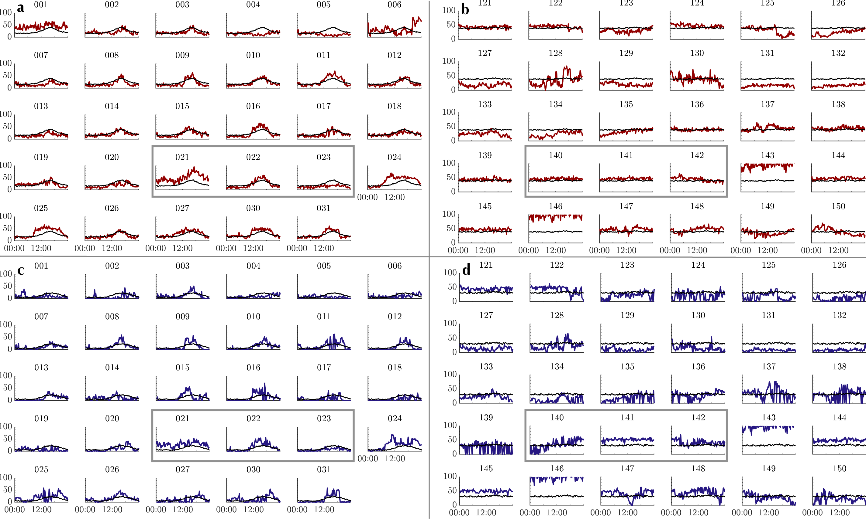
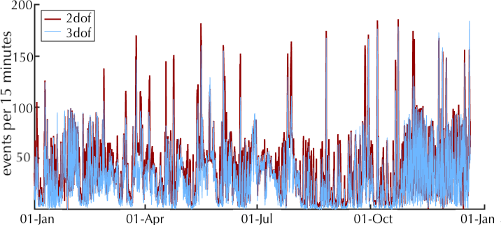

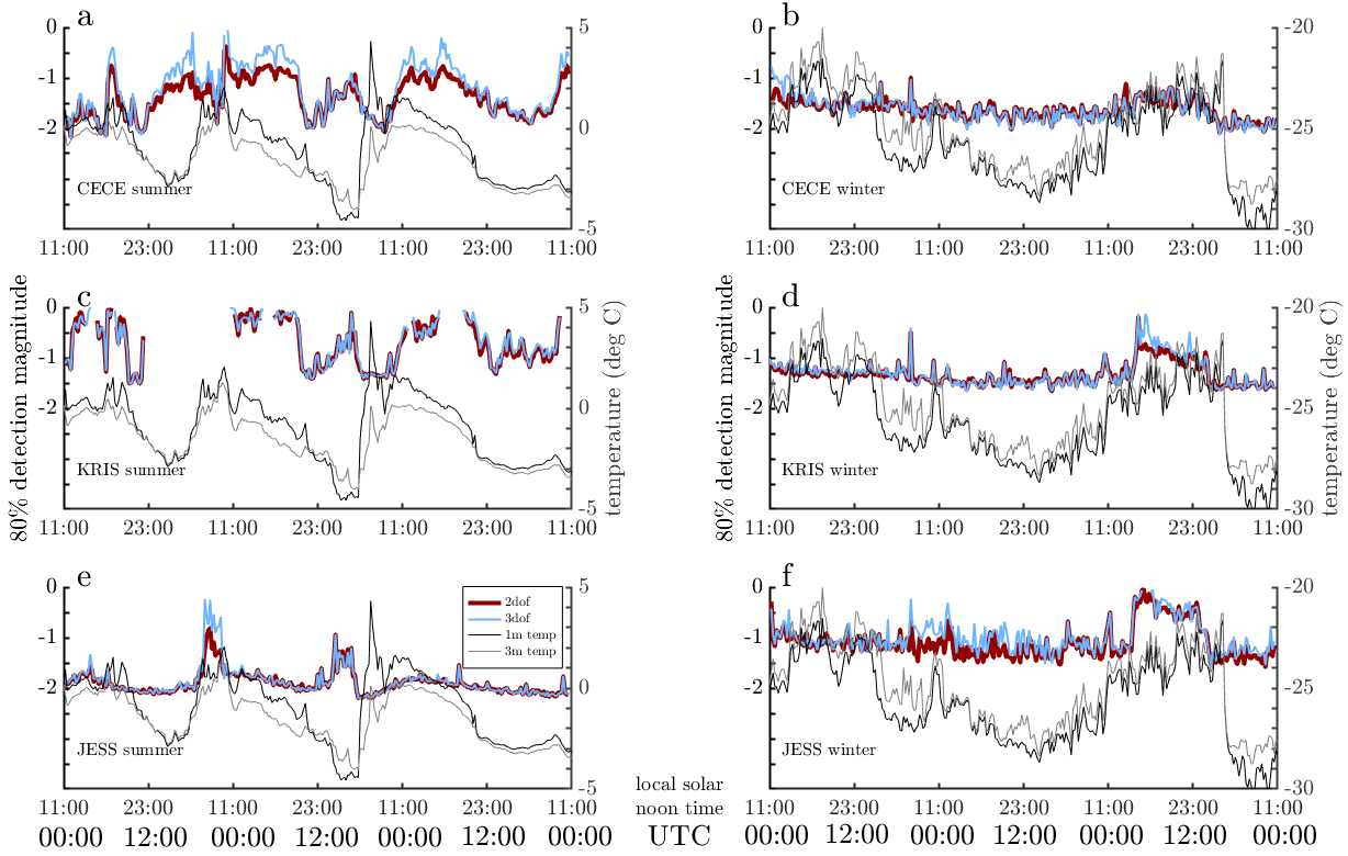


 Open access