


1. Introduction
The Arctic is a critically important component of the Earth's climate system, affecting the energy balance, atmospheric and oceanic circulations, ecology and natural resources (Callaghan and others, Reference Callaghan, Johansson, Prowse, Olsen and Reiersen2011; Olsen and others, Reference Olsen2011). With global warming, the periphery of the Arctic sea-ice cover has undergone significant changes, with a reduction in sea-ice extent, a shift from multiyear to first-year ice and thus a thinner ice pack (Nghiem and others, Reference Nghiem2007; Stroeve and others, Reference Stroeve, Markus, Boisvert, Miller and Barrett2014). During the melting period in the Arctic, meltwater gathers in depressions on the ice surface and then develops to form melt ponds. The ratio between the melt pond area and sea-ice area (per gridcell) is called the melt pond fraction (MPF) (Rösel and others, Reference Rösel and Kaleschke2012; Kern and others, Reference Kern2016). Melt ponds have lower albedo compared with snow and ice surface, leading to the increase in the absorption of solar radiation and hence the acceleration of sea-ice melt (Flocco and Feltham, Reference Flocco and Feltham2007). This process is known as ice-albedo feedback, which plays an important role in the warming process in polar regions (Skyllingstad and others, Reference Skyllingstad, Paulson and Perovich2009; Serreze and Barry, Reference Serreze and Barry2011). In addition, the development of melt ponds increases the permeability of ice, heats the upper ocean and changes the heat budget of the mixed layer (Eicken and others, Reference Eicken, Krouse, Kadko and Perovich2002). The permeation of the bottom of the melt pond removes salt from sea ice. Latent heat release during the freezing of melt ponds affects the growth of the bottom of the sea ice. Therefore, melt pond evolution plays an important role in the heat and mass budget of sea ice and the polar climate.
In situ observations and numerical models are important means to study melt ponds. However, the natural environment of the Arctic is unfavourable, resulting in difficulty in conducting in situ observations. Numerical models cannot simulate the evolution of melt pond coverage in detail very well (Taylor and Feltham, Reference Taylor and Feltham2004; Flocco and Feltham, Reference Flocco and Feltham2007). Remote-sensing technology is becoming an effective means to monitor melt ponds. Tschudi and others (Reference Tschudi, Maslanik and Perovich2008) estimated the MPF at the basin scale using the linear mixture model based on the Moderate Resolution Imaging Spectroradiometer (MODIS) data. This method is simple, easily understood and hence widely used. Rösel and others (Reference Rösel and Kaleschke2012) improved this method by adding the linear mixture model to the artificial neural network. The generated MPF products achieved an 8-day temporal resolution during the melting period in the Arctic from 2000 to 2011 based on MODIS reflectance data. Considering the different reflection characteristics of different types of melt ponds, Yackel and others (Reference Yackel2017) improved this method by distinguishing different types of ponds to improve the accuracy of MPF retrieval. The mechanisms of melt pond formation and evolution were studied using field data, showing a great difference in melt ponds on first-year and multiyear ice (Eicken and others, Reference Eicken, Krouse, Kadko and Perovich2002; Polashenski and others, Reference Polashenski, Perovich and Courville2012). As an important site in the Arctic, melt ponds on first-year sea ice in the Canadian Arctic Archipelago (CAA) have been investigated in many studies (Yackel and Barber, Reference Yackel and Barber2000; Yackel and others, Reference Yackel and Barber2000; Scharien and Yackel, Reference Scharien and Yackel2005; Jack and others, Reference Jack, Jens, Megan and David2014). However, few studies investigated melt ponds both on first-year and multiyear ice in the CAA (Scharien and others, Reference Scharien2017). Most of the previous studies have used low- and medium-resolution satellite remote-sensing data to detect melt ponds over a wide range and long time or carried out a small range of short-time melt pond extraction based on high-resolution optical data (Rösel and Kaleschke, Reference Rösel and Kaleschke2012; Rösel and others, Reference Rösel, Kaleschke and Birnbaum2012; Istomina and others, Reference Istomina2015; Miao and others, Reference Miao, Xie, Ackley, Perovich and Ke2015). However, melt ponds are generally small and change rapidly. Therefore, it is necessary to use remote-sensing data with high spatial and temporal resolutions to monitor melt ponds on different types of sea ice during the entire melting period in the CAA.
In this study, we monitored melt ponds on first-year and multiyear ice separately with optical satellite data of the CAA. First, the accuracy of the fully constrained least-squares (FCLS) algorithm was evaluated by using a WorldView-2 image. Then, MPF retrieval was carried out in the summer of 2017 based on Sentinel-2 and Landsat 8 reflectance data. This is followed by a discussion of the evolution of melt ponds on first-year and multiyear ice and its relationships with air temperature and albedo.
2. Study sites and dataset
2.1 Study sites
The CAA is an essential part of the Northwest Passage (NWP), and sea-ice melt is important for studying the navigability of the NWP. The Queen Elizabeth Islands are the northernmost archipelago in the CAA, where there are 34 large islands and 2092 small islands, with a total area of 4.2 × 10⁵ km2. The first-year ice near Melville Island and the multiyear ice near Mackenzie King Island were selected as the study sites, and the algorithm validation was conducted near the first-year ice study area (Fig. 1). First-year and multiyear sea ice were distinguished based on Sentinel-2 and Landsat 8 images. Sea ice in the first-year ice study site grew in the fall and winter of 2016 and did not survive the summer of 2017, whereas sea ice in the multiyear ice study site had survived at least one melt season. The study sites are both in the channels and straits of the CAA, which are covered with land-fast ice (Yu and others, Reference Yu, Stern, Fowler, Fetterer and Maslanik2013; Mahoney, Reference Mahoney2018). This allows long time-series measurements of melt ponds on sea ice.
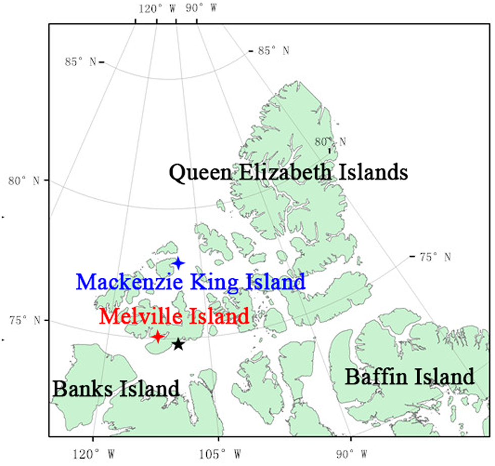
Fig. 1. Overview of the study areas in the CAA. The blue star shows the location of the multiyear ice study site, the red star shows the location of the first-year ice study site, and the black star shows the location of the test site for algorithm accuracy.
2.2 Dataset
The experimental data include the WorldView-2 Ortho Ready Standard 2A product, Sentinel-2 Level-1C product, Landsat 8 Level-2 surface reflectance product and ERA-Interim 2 m temperature reanalysis data. WorldView-2 was launched on 2 October 2009 and can provide panchromatic imagery at 0.5 m spatial resolution and 8-band multispectral imagery at 1.8 m spatial resolution (Eugenio and others, Reference Eugenio, Martin, Marcello and Bermejo2013). Sentinel-2A and Sentinel-2B were launched on 23 June 2015 and 7 March 2017, respectively. These two satellites together provide global coverage of the Earth's land surface every 5 days. The imagery is 13-band data in the visible, near-infrared and short-wave infrared parts of the electromagnetic spectrum, and the spatial resolution ranges from 10 to 60 m (Li and Roy, Reference Li and Roy2017). The European Space Agency has released L1C multispectral data with geometric precision correction. Landsat 8 was launched on 11 February 2013, covers land surfaces between 83°N and 83°S and can provide multispectral imagery at 30 m spatial resolution, panchromatic imagery at 10 m spatial resolution and additional thermal infrared imagery at 100 m spatial resolution with a temporal resolution of 16 days (Ko and others, Reference Ko, Kim and Nam2015). The Landsat 8 Level-2 surface reflectance product is a secondary product officially issued by the United States Geological Survey. ERA-Interim is a global reanalysis dataset produced by the European Centre for Medium-Range Weather Forecasts. This study uses ERA-Interim 2 m temperature reanalysis data with a grid spacing of 0.125°.
During the melting period, melt ponds can appear in any place where sea ice exits as long as the conditions of the formation of melt ponds are met. Thus, melt ponds may appear on sea ice in the high Arctic. However, Landsat imagery covers land surfaces to a certain latitude and therefore is not usable for large-scale observations in the high Arctic. Consequently, it is not suitable to use Landsat 8 images to monitor melt ponds on sea ice in the high Arctic. In addition, melt ponds are generally small and change rapidly. However, Sentinel-2 imagery is available on a global scale with a high spatial resolution every 5 days, showing the potential in monitoring melt ponds on sea ice in the Arctic. In this study, all the study sites are located at below 83°N, which can be observed by both Landsat 8 and Sentinel-2 sensors. Thus, Sentinel-2 and Landsat 8 images were used in combination to improve the temporal resolution in monitoring melt ponds. In this study, the average temporal resolution could reach 12 days, and the resolution was up to 1 day during some stages of melt ponds. This was helpful to better study the evolution of melt ponds on sea ice.
WorldView-2 imagery with a high spatial resolution can be used to accurately detect the size and position of the melt pond. Therefore, melt ponds mapped by WorldView-2 image were used to evaluate the reliability of the FCLS algorithm in MPF retrieval. Twenty-three high-quality Sentinel-2 and Landsat 8 images from May to September 2017 were selected to effectively detect melt ponds and investigate the seasonal evolution of melt ponds.
3. Methodology
3.1 Data processing flow
The data processing flow is shown in Figure 2. First, we mapped the high-resolution melt pond distribution from the WorldView-2 image based on supervised classification. Second, the Sentinel-2 L1C product was processed with radiation calibration and atmospheric correction to obtain the surface reflectance data and the cloud mask. The Landsat 8 Level-2 surface reflectance product contains cloud masks and saturated masks. Then, high-quality surface reflectance data were generated by applying the masks to Sentinel-2 and Landsat 8 surface reflectance data. A sample library was established by selecting numerous sample points that were distinguished by comparative interpretation. According to the spectral reflectance characteristics of different surface features, the abundance of different surface features was retrieved by the FCLS algorithm, and hence, the melt pond coverage distribution was obtained. The accuracy of MPF retrieval by the FCLS algorithm was evaluated by comparing with the corresponding WorldView-2 MPF retrieval. The air temperature in the study areas was obtained from ERA-Interim reanalysis data, and the surface broadband albedo was calculated using the narrow-to-broadband conversion formula. Last, we compared the evolution of melt ponds, together with the air temperature and surface albedo, on first-year ice and multiyear ice.
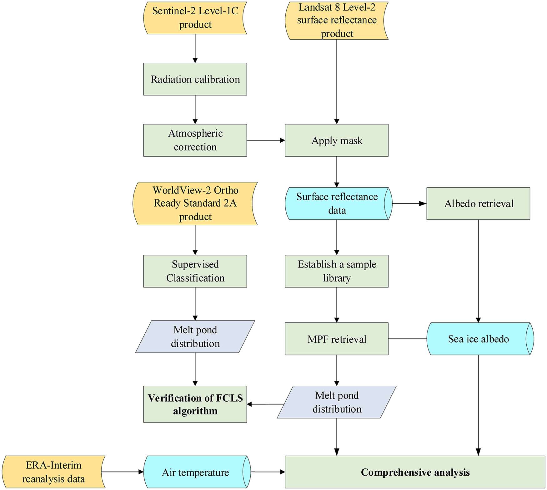
Fig. 2. Data processing flow.
3.2 FCLS algorithm
Melt ponds are usually smaller than a pixel in the Sentinel-2 and Landsat 8 images. The mixed-pixel decomposition is used to solve the problem of soft classification and obtain the types of pure surface features in each pixel of remote-sensing data and their proportion coefficient (abundance) (Keshava and Mustard, Reference Keshava and Mustard2002; Bioucas-Dias and others, Reference Bioucas-Dias2012). A sea-ice pixel consists of three surface features: open water, melt pond and sea ice. The reflectance at each pixel is determined by a weighted linear combination of the reflectances of these three features and their abundances (Istomina and others, Reference Istomina2015). Based on the spectral reflectance characteristics of different surface features, the reflectances of the near-infrared, red and blue bands are used to retrieve abundance. The linear mixed model is expressed as follows (Heinz and Chang, Reference Heinz and Chang2002; Tschudi and others, Reference Tschudi, Maslanik and Perovich2008):

where W, M and I represent open water, melt pond and sea ice, respectively; i, j and k represent different bands; r(λ)is the reflectance of different features in different bands; A i represents the abundance of different surface features; n is noise or can be interpreted as a measurement error; and R(λ) represents the reflectance value of the pixel in different bands. In order to guarantee the obtained reflectances of different features are closest to that of the actual features, r(λ) of different features in each image were determined from the average of the corresponding sample in this image.
The abundance may be >1 or <0 in Eqn (1). Therefore, the constraint conditions of the sum-to-one and non-negative abundances are added to ensure that the solution process becomes more reasonable:
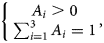
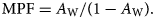
Eqns (1) and (2) are solved simultaneously to obtain the abundances of open water, melt pond and sea ice. The set of Eqns (1) and (2) contains three unknown values (A W, A M, A I) in five equations, therefore the equations are overdetermined. It is possible that there is more than one exact solution. Therefore, we consider this as an optimization problem and find the optimal solution by using a least-square method (Rösel and others, Reference Rösel and Kaleschke2012). Melt ponds only exist on sea ice, and the influence of open water should be excluded from the analysis. Therefore, the formula of the MPF is shown as follows:
3.3 Albedo retrieval
Sea-ice albedo is crucial to determine the amount of energy absorbed by oceans throughout the year. Especially in summer, when melt ponds appear on sea ice, the sea-ice albedo drops and substantially impacts on sea-ice melt rates. Therefore, it is important to explore the relationship between melt ponds and sea-ice albedo. However, few products contain albedo over the ocean and sea-ice surfaces. The current products only contain albedo over the land surfaces and that the albedo over the ocean and sea-ice surface is usually left blank (Ying and others, Reference Ying2015). Although ERA-Interim contains albedo reanalysis data, the resolution is too low to study melt pond. Hence, the sea-ice albedo of the corresponding time and region was calculated based on the narrow-to-broadband conversion formula (Naegeli and others, Reference Naegeli2017):

where ∂ represents the surface albedo; S and L refer to Sentinel-2 and Landsat 8 imagery, respectively; and b i corresponds to the reflectance of the ith band.
This formula is one of the most commonly applied narrow-to-broadband conversion formulae. It is based on extensive radiative transfer simulations that incorporated 256 surface reflectance spectra and the atmospheric conditions (Liang, Reference Liang2001). The validation results show that the conversion formulae are very accurate with an average residual standard error of ~0.02 (Liang and others, Reference Liang2002). To eliminate the influence of open water on sea-ice albedo, we calculated the albedo of pixels with an open water abundance of zero in this study.
4. Results and analysis
4.1 Verification of the FCLS algorithm
High-resolution WorldView-2 imagery was selected as validation data to evaluate the accuracy of the FCLS algorithm in MPF retrieval. The verification process required WorldView-2, Sentinel-2 and Landsat 8 imagery to simultaneously cover the same area. This condition is difficult to satisfy because the three satellites have different repeat cycles, and optical images are frequently affected by clouds. Thus, three images (Landsat 8 images on 4 July 2017 and WorldView-2 and Sentinel-2 images on 5 July 2017) covering the same area near the first-year ice study area were selected as experimental data for algorithm verification. We used multispectral Landsat 8 image with 30 m resolution and multispectral Sentinel-2 image with 10 m resolution. WorldView-2 image was resampled to 1.5 m resolution.
The support vector machine (SVM) is a supervised learning model with associated learning algorithms that analyse data used for classification. This method is widely used in supervised classification due to its ability to successfully handle small training datasets, often showing higher classification accuracy than the traditional methods (Mantero and others, Reference Mantero, Moser and Serpico2005; Mountrakis and others, Reference Mountrakis, Im and Ogole2011). Thus, we chose SVM to supervise the classification of the WorldView-2 image based on the Environment for Visualizing Images (ENVI) platform (Fig. 3b) and ensured the independence of the reference value. The pixel in WorldView-2 image with a high spatial resolution was considered as a pure pixel. There was no open water in the experimental area on 5 July 2017 for FCLS algorithm validation. Therefore, the pixels in WorldView-2 image were classified as melt pond and sea ice. The FCLS algorithm was used to retrieve the MPF by Sentinel-2 image and Landsat 8 image (Figs 3c and d). The melt pond distributions derived from the three images agree with each other well.

Fig. 3. (a) The 7.2 km × 7.2 km subset (band combination 5-3-2) from the WorldView-2 image. This subset is used for FCLS algorithm validation. (b) The MPF of the WorldView-2 subset determined with the SVM. Blue areas are melt ponds, and white areas are sea ice. (c) The MPF determined from Sentinel-2. The coordinates are the gridcell numbers. (d) The MPF determined from Landsat 8. The coordinates are the gridcell numbers.
Regression analysis and root mean square error (RMSE) were used to quantitatively evaluate the accuracy of the FCLS algorithm in MPF retrieval. With 6 × 6 as the statistical unit in Landsat 8 image, the MPF was the average of MPFs in each unit. Correspondingly, 18 × 18 was the statistical unit in Sentinel-2 image and 120 × 120 was the statistical unit in WorldView-2 image. In Sentinel-2 image, the MPF was the average of MPFs in each unit. In WorldView-2 image, the number of pixels classified as melt pond was calculated and then divided by the total number of pixels to compute MPF. This was used to be the reference value for evaluating the accuracy of the FCLS algorithm in MPF retrieval using Sentinel-2 and Landsat 8 images. As shown in Figure 4, the point distribution was concentrated near the line y = x, showing an apparent linear trend. The correlation coefficients were all >0.8, indicating that the MPFs determined from Sentinel-2 and Landsat 8 were highly consistent with the reference value. The RMSE of the MPF determined from Sentinel-2 was only 0.06, and that from Landsat 8 was 0.16. This was because the Landsat 8 image was acquired 1 day before the two other images were acquired, and the melt pond changed over time. A high correlation coefficient and a low RMSE indicated that the FCLS algorithm had a high accuracy in MPF retrieval, suggesting that the FCLS algorithm is an effective method to retrieve the MPF.
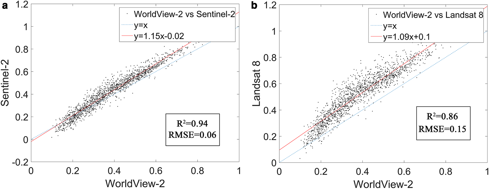
Fig. 4. Comparison of the MPFs determined from (a) WorldView-2 and Sentinel-2 and (b) WorldView-2 and Landsat 8. The red line shows a least-square linear regression, and the blue line shows a 1:1 relation.
4.2 Comparison of the MPFs determined from Sentinel-2 and Landsat 8
In the multiyear ice study site, the Sentinel-2 images were resampled to the same resolution as the Landsat 8 images (30 m) on 17 August 2017. Then, the MPFs determined from two images were compared. Figure 5 illustrates that the MPF distributions from Sentinel-2 and Landsat 8 were similar (Figs 5c and d). The scatter density map (Fig. 5e) shows that the distribution concentration of the points had an apparent linear trend, the root mean square deviation was 0.07, and the R 2 value was 0.72. The histogram of the difference between the MPFs of Sentinel-2 and Landsat 8 (Fig. 5f) presents a normal distribution, and most values are concentrated around zero, indicating that the difference between the two results was very small. Therefore, our results suggest that the MPFs determined from Sentinel-2 and Landsat 8 are consistent with each other.

Fig. 5. (a) True-colour subset (band combination 3-2-1) from the Sentinel-2 image. (b) True-colour subset (band combination 4-3-2) from the Landsat 8 image. (c) The MPF of the Sentinel-2 subset determined with FCLS. (d) The MPF of the Landsat 8 subset determined with FCLS. (e) Comparison of MPFs determined from Sentinel-2 and Landsat 8. (f) Histogram of the difference between the MPFs of Sentinel-2 and Landsat 8.
4.3 Evolution of melt pond coverage on different types of sea ice
Previous studies have demonstrated that the evolution of melt ponds can be characterized by four general stages, depending on the pond behaviour and control mechanisms (Eicken and others, Reference Eicken, Krouse, Kadko and Perovich2002; Polashenski and others, Reference Polashenski, Perovich and Courville2012). In this study, the differences in pond evolution on first-year and multiyear ice at four stages were analysed and compared. Figure 6 shows the time series of the melt pond coverage and open water coverage in first-year and multiyear ice area during the melting period in 2017.
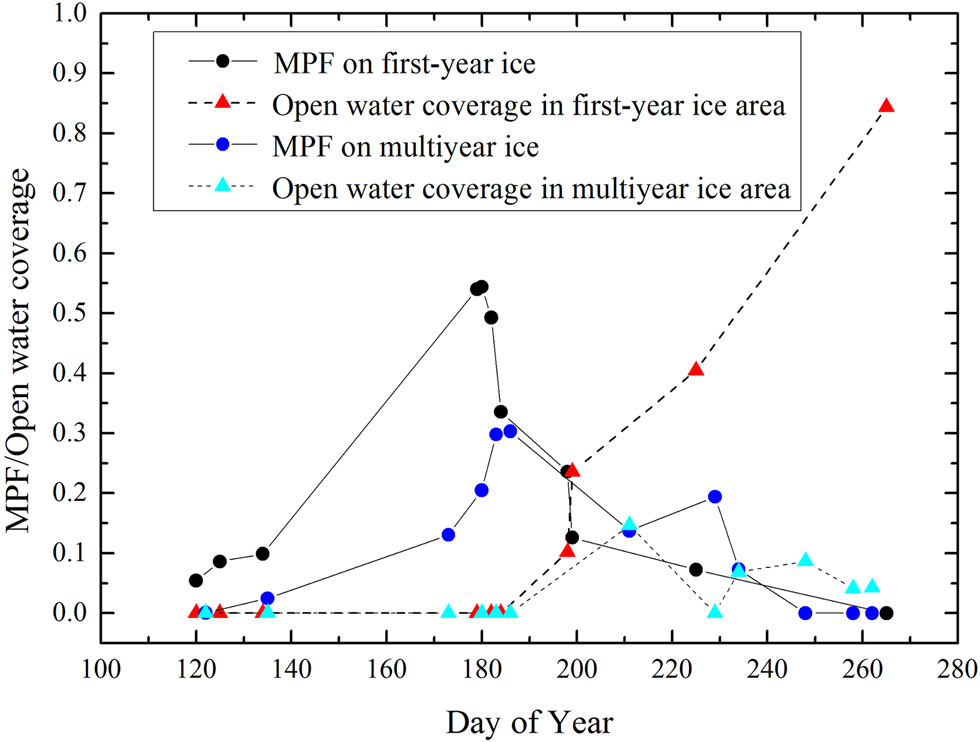
Fig. 6. Time series of the MPF and open water coverage in first-year and multiyear ice area derived from Sentinel-2 and Landsat 8.
The first stage begins with the onset of pond formation and is characterized by widespread ponding as meltwater accumulates on the surface of relatively impermeable ice. This stage in the first-year ice study area ranged from day of year (DOY) 120 to 180, and multiyear ice ranged from DOY 122 to 186 (Fig. 6). The snow began to melt, and a significant lateral transport of meltwater drained into cracks and other flaws (Eicken and others, Reference Eicken, Krouse, Kadko and Perovich2002). The distribution and coverage of melt ponds are affected by the topographic relief of ice. Due to the topographic relief created by hummocks, melt ponds on multiyear ice tend to be confined to deeper and smaller ponds than those on first-year ice, where limited relief results in shallow but large ponding. Figures 7a and b show the images when the melt pond coverage on first-year and multiyear ice reached a maximum. Most melt ponds on first-year ice were shallow and flat, and the colour was dark blue and grey, whereas most melt ponds on multiyear ice were deeper and more complex geometrical patterns, and the colour was bright blue (Polashenski and others, Reference Polashenski, Perovich and Courville2012; Webster and others, Reference Webster2015; Lu and others, Reference Lu2018). This was because that the colour gradually changed from dark blue to bright blue with increasing underlying ice thickness (Lu and others, Reference Lu2018). At this stage, the surfaces of the melt ponds are usually higher than the sea level, and hence, the pressure head is positive. However, the meltwater can refreeze due to a low ice temperature. Consequently, the permeability of sea ice is small, and the access of the meltwater to open water is limited, resulting in an increase in melt pond coverage. At the end of the first stage, the melt pond coverage reached a seasonal maximum of 54% on first-year ice on DOY 180 and only 30% on multiyear ice on DOY 186. It was obvious that the max peak of MPF on first-year ice was earlier than multiyear ice. This was affected by air temperature. According to the air temperature data, the temperature in first-year ice area reached a maximum of 9°C on DOY 182, which was earlier than multiyear ice area where the temperature reached a maximum of 6°C on DOY 185.

Fig. 7. Melt ponds on (a) first-year ice on 30 June 2017 and (b) multiyear ice on 5 July 2017.
During the second stage, the melt pond coverage decreased substantially on first-year ice but only decreased slightly on multiyear ice (Polashenski and others, Reference Polashenski, Perovich and Courville2012). This stage in the first-year ice study area ranged from DOY 181 to 198, as shown in Figure 6, and ranged from DOY 187 to 211 for multiyear ice. The drainage of meltwater increased. As the ice temperature increased, the permeability of sea ice increased, resulting in percolation through the ice (Eicken and others, Reference Eicken, Grenfell, Perovich, Richter-Menge and Frey2004). In addition, the horizontal transport of meltwater led to an interconnected system of streams and ponds, resulting in an increased outflow through macroscopic flaws (Scharien and Yackel, Reference Scharien and Yackel2005). At the end of the second stage, melt ponds remained very near sea level, the production and loss of meltwater were generally equal, and the shapes of the melt ponds were also finally fixed.
During the third stage, the melt pond coverage on multiyear ice slowly increased (from DOY 212 to 229, Fig. 6). Given the lack of images, the increase in the melt pond coverage on first-year ice was not observed. However, the optical images show the morphological changes in the melt ponds in the first-year ice study area, which could be used to infer that the third stage of the melt ponds on first-year ice occurred during the period from DOY 199 to 225. At this stage, the sea-ice permeability reaches its maximum, the pressure head remains at sea level and the outflow is small (Eicken and others, Reference Eicken, Krouse, Kadko and Perovich2002). The pond area increased by creating new areas where the local surface height was below freeboard. These areas may be created by lateral melt at the walls of the ponds (Polashenski and others, Reference Polashenski, Perovich and Courville2012).
The fourth stage, refreezing, is not restricted to the end of the season. This phenomenon can occur at any time during the melting period because the changes in atmospheric forcing may result in freezing conditions. The melt pond coverage on first-year and multiyear ice decreases to zero, and melt ponds refreeze, or sea ice breaks up. This stage in the first-year ice study area took place starting on DOY 226, and multiyear ice took place starting on DOY 230 (Fig. 6). The open water disappeared in the multiyear ice study area, whereas the open water coverage in the first-year ice study area exceeded 80% because the first-year ice thickness was too shallow to withstand severe melting, causing the ice to break up. However, melt ponds on multiyear ice refreeze from the surface.
During the entire melting period, the melt pond coverage on first-year ice changed dramatically, whereas that on multiyear ice remained relatively flat. The evolution of the melt ponds differs based on sea-ice type.
4.4 Relationships of the MPF with air temperature and albedo
In this study, we adopted the following criteria for determining the melt onset and the end of melting dates. The 0°C is the point as an indicator of whether it is melting. Considering that melting usually happens faster than freezing, the windows were selected for 3 and 7 days, respectively, to filter erroneous information. Therefore, melt onset is considered to be occurring when the temperature exceeds 0°C for three consecutive days, whereas the first day of the seven consecutive days below 0°C after the melting period is considered as the end of melting (Kunz and Long, Reference Kunz and Long2006). These criteria achieved a filtering effect and could remove erroneous information about freeze–thaw to a certain extent. Figure 8a shows that the temperature in the first-year ice study area exceeded 0°C for three consecutive days starting on DOY 164, and the end of melting occurred on DOY 242. Therefore, the melting period in this area ranged from DOY 164 to 242. Similarly, Figure 8b shows that the melting period in the multiyear ice study area ranged from DOY 163 to 238. This was similar to the melting period of first-year ice because the study areas of first-year and multiyear ice were close to each other and had similar characteristics. However, melt ponds appeared on sea ice before melt onset. The melt pond coverage was small and <10%. Then, melt ponds developed rapidly after melt onset, resulting in a sharp increase in coverage. After the end of melting, the coverage dropped to zero.
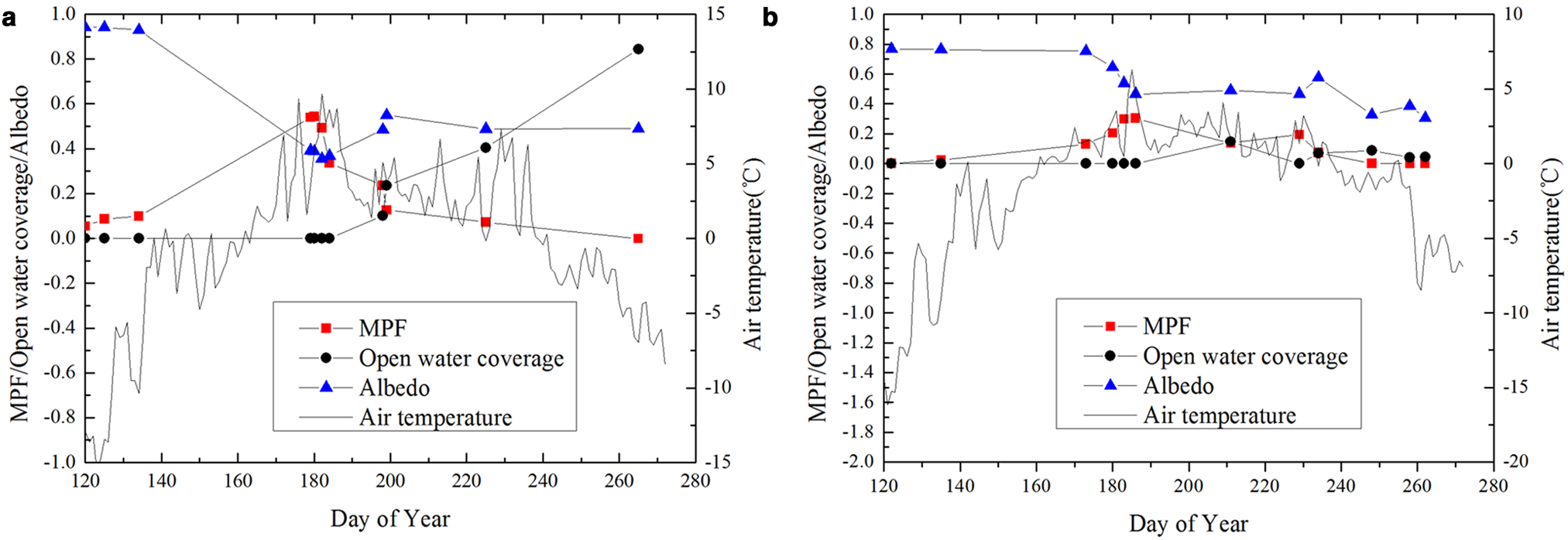
Fig. 8. Time series of the MPF, open water coverage, albedo and air temperature in (a) first-year ice area and (b) multiyear ice area.
Figure 8 shows that the first-year ice albedo curve initially declined, increased, decreased again and increased during the melting period. However, the trend was opposite to the change trend of the melt pond coverage curve in general, and some points were abnormal. Whereas, the trend of the multiyear ice albedo was completely opposite to that of the melt pond coverage curve. Here, two images from first-year and multiyear ice study area on DOY 179 (29 June 2017), respectively, were selected for studying the relationship between the MPF and the sea-ice albedo. In both first-year and multiyear ice, there was a significantly negative correlation (R = −1) and a high significance level (p < 0.01) between the sea-ice albedo and the melt pond coverage (Fig. 9). These findings indicated that the appearance of melt ponds on both first-year and multiyear ice reduced the sea-ice albedo and that the melt pond coverage was an important factor affecting the change in sea-ice albedo during the melting period. Subsequently, melt ponds disappeared, the sea ice began to freeze and the albedo gradually increased.

Fig. 9. Relationship between the MPF and albedo on (a) first-year ice and (b) multiyear ice on 29 June 2017.
In addition, there was no obvious same or opposite trend between open water coverage curve and air temperature curve in Figure 8. This is because that the formation of open water is affected by many factors. It depends on the combined effects of many factors such as air temperature, the amount of meltwater, sea-ice thickness, sea-ice deformation, etc. During the first stage, the temperature rose gradually and the amount of meltwater increased dramatically, resulting in an increasing MPF. However, the open water coverage was near zero. This was because that meltwater gathered in depressions on the ice surface and the main mode of transport was lateral transport, which was not helpful for the formation of open water. During the fourth stage, the temperature dropped gradually and the amount of meltwater decreased dramatically. In first-year ice area, the open water coverage increased to more than 80% because the ice thickness was too shallow to withstand severe melting, causing the ice to break up. Whereas, in multiyear ice area, the ice thickness could withstand severe melting and then melt ponds on multiyear ice refroze from the surface. Hence, there was no much open water generated.
5. Discussion
The validation of the MPFs of Sentinel-2 and Landsat 8 with WorldView-2 high-resolution image shows a high correlation coefficient (R 2 > 0.8) and a low RMSE (RMSE < 0.16). This demonstrates that the FCLS algorithm performs well in MPF retrieval. However, we assume that a pixel consists of three surface features (open water, melt pond and sea ice), which may cause uncertainties since the Arctic sea ice is actually covered by various surface types rather than only three types (Rösel and Kaleschke, Reference Rösel and Kaleschke2012; Rösel and others, Reference Rösel and Kaleschke2012). For example, there are at least five types of melt ponds during the melting period (Yackel and others, Reference Yackel2017). Furthermore, it is necessary to consider more classes like melt ponds with different types, wet snow, bare ice or sediment-laden surfaces (Rösel and others, Reference Rösel and Kaleschke2012).
The Sentinel-2 and Landsat 8 images were used in combination to calculate the MPF in order to improve the temporal resolution in monitoring the evolution of melt ponds. Although the MPFs determined from Sentinel-2 and Landsat 8 show good agreement with an RSMD of 0.07, there were still errors from different sensors, spatial resolutions and geolocation error.
There were significant differences in melt ponds between first-year and multiyear ice. The melt pond coverage on first-year ice changed dramatically, whereas that on multiyear ice remained relatively flat. Melt ponds on multiyear ice were deeper with less spatial coverage than on first-year ice where limited relief results in shallow and large ponding. This agrees with the description of Polashenski and others (Reference Polashenski, Perovich and Courville2012).
The seasonal maximum of the MPF on first-year ice during the melting period is 54%, which is less than the MPF determined from MODIS melt pond dataset, showing 70% at the end of June on the flat first year ice in the CAA (Rösel and others, Reference Rösel and Kaleschke2012). Melt ponds are usually small and change rapidly. Due to the strong diurnal cycle of melt-water production rates, intra-daily variations in the MPF can occur at least during the first stage of melt ponds (Eicken and others, Reference Eicken, Grenfell, Perovich, Richter-Menge and Frey2004). Therefore, the observed differences between our results and MODIS melt pond dataset may result from the different spatial resolutions and observation time.
We confirm that the MPF increased rapidly after melt onset, and then dropped to zero after the end of melting. However, few melt ponds appeared on sea ice before melt onset in this study. The results may be due to the uncertainties in ERA-Interim 2 m temperature reanalysis data and the representativeness errors. Additionally, solar radiation can penetrate and warm the snow cover with a low thermal conductivity. This elevated sub-surface temperature allows a layer of wet snow to form below the surface even on days when the air temperature remains sub-freezing (Koh and Jordan, Reference Koh and Jordan1995).
Our results show a significantly negative correlation (R = −1) between the MPF and sea-ice albedo. The so-called ice-albedo feedback is one of the dominated factors of polar climate (Skyllingstad and others, Reference Skyllingstad, Paulson and Perovich2009; Serreze and Barry, Reference Serreze and Barry2011). Figure 8a shows the variations of the first-year ice albedo were opposite to that of the melt pond coverage curve in general. However, some points were abnormal. Further analysis is needed. Here, two images from the first-year ice study area were selected for further analysis. The opposite trend point occurred at DOY 180 (30 June 2017), and the abnormal point occurred at DOY 225 (14 August 2017). In both cases, the sea-ice albedo and the melt pond coverage show a significantly negative correlation (R > −0.9) and a high significance level (p < 0.01) (Fig. 10). These findings indicate that the melt pond coverage was still an important factor affecting sea-ice albedo at this abnormal point. A possible reason for the abnormal point was that the salt crystal precipitation or the presence of other impurities during the melting process of first-year ice affected the sea-ice albedo (Carns and others, Reference Carns, Brandt and Warren2016). Consequently, the change in sea-ice albedo was not completely consistent with the change trend of melt pond coverage.

Fig. 10. Relationship between the MPF and albedo on first-year ice on (a) 30 June 2017 and (b) 14 August 2017.
Our results indicate that the MPF determined from Sentinel-2 is consistent with that from WorldView-2. In addition, Sentinel-2 imagery is available on a global scale with a high spatial resolution every 5 days, showing the potential in monitoring melt ponds on sea ice in the Arctic. The further work will try to monitor melt ponds for long time based on the proposed method.
6. Conclusion
The evolution of melt ponds on sea ice is important for the polar climate system, as it can affect surface albedo and plays an important role in the surface heat budget. The MPF is a key parameter for estimating the rate of sea-ice melt in summer. The FCLS algorithm can be used to estimate the summer MPF based on Landsat-8 and Sentinel-2 images and shows good performance when compared with the results derived from WorldView-2. Melt ponds on first-year and multiyear ice in the CAA in 2017 were monitored based on Sentinel-2 and Landsat 8 images at a high temporal resolution. The relationships of melt pond coverage with air temperature and albedo were analysed.
During the first stage, the melt ponds on first-year ice developed rapidly, and the melt pond coverage was able to exceed 54%. However, the melt pond coverage on multiyear ice slowly increased, with only ~30% at its peak. During the second stage, the pond coverage declined due to the rapid drainage of meltwater by horizontal transport and percolation through the ice. During the third stage, the pond coverage experienced steady growth by the lateral melt at the walls of the ponds. During the fourth stage, the first-year ice began to break up, and the melt ponds on multiyear ice refroze. During the entire melting period, the melt pond coverage on first-year ice changed dramatically, whereas the melt pond coverage on multiyear ice remained relatively flat. The evolution of melt ponds is different between first-year and multiyear sea ice. A significantly negative correlation is found between sea-ice albedo and melt pond coverage during the melt season. Afterward, the melt ponds disappear. The sea ice starts to refreeze, and the albedo gradually increases.
With global warming, there have been significant changes in sea ice in the Arctic. Melt ponds on sea ice on large scale deserve our attention because of ice-albedo feedback. In addition, melt ponds are generally small and change rapidly. Studying the evolution of melt ponds in detail can potentially help the modelling of melt pond evolution and provide new opportunities to parameterize ponds. Therefore, it is important to studying melt ponds evolution in detail on large scale. However, the spatial resolution of Sentinel-2 and Landsat 8 data is limited. Although the combination of the two data sources improves the temporal resolution to a certain extent, it is still not sufficient for studying the evolution of melt ponds in detail on large areas. Melt ponds will need to be further monitored in more detail using our data combined with optical data with a sub-metre resolution, aerial photographs and field measurement.
Acknowledgements
This research is funded by the National Key Research and Development Program of China (2018YFC1406102), the National Natural Science Foundation of China (NSFC) (41776200, 41531069) and the Funds for the Distinguished Young Scientists of Hubei Province (China) (2019CFA057).


 Open access