The Exponential-Centred Skew-Normal Distribution

Abstract

Data from some research fields tend to exhibit a positive skew. For example, in experimental psychology, reaction times (RTs) are characterised as being positively skewed. However, it is not unlikely that RTs can take a normal or, even, a negative shape. While the Ex-Gaussian distribution is suitable to model positively skewed data, it cannot cope with negatively skewed data. This manuscript proposes a distribution that can deal with both negative and positive skews: the exponential-centred skew-normal (ECSN) distribution. The mathematical properties of the proposed distribution are reported, and it is featured in two non-synthetic datasets.

1. Introduction

Hohle [1] used the convolution between two random variables, exponential and Gaussian, to model simple reaction times (RTs) elicited via psychological experiments. The distributions resulting from such convolutions are known as exponential-Gaussian distributions or, simply, Ex-Gaussian (EG) distributions. Other distributions, though, have been proposed to model RT data. For example, it has been shown that the shifted Wald, shifted Birnbaum–Saunders [2] and shifted Gamma distributions [3] provide good fits to RT data (the Birnbaum–Saunders distribution has also been used to model neural activity [4], and a flexible version of it was proposed recently [5]. The slashed quasi-Gamma distribution (an extension of the generalised Gamma distribution) has been proposed to model data with varying skewness and high kurtosis [6]. To our knowledge, neither the flexible Birnbaum–Saunders nor the slashed quasi-Gamma distributions have been tested in the modelling of RT data; hence, this is a task for future research). Nonetheless, distributions of RTs resulting from psychological experiments are commonly adjusted with the EG distribution model.

EG distributions were first introduced in an RT analysis carried out by McGill [7], who, when studying the RT cumulative distribution function as a result of different intensities of auditory stimuli, found that they had an exponential form with similar constant times. This led to the assumption that, at least, one component of the total RT had an exponential distribution, and since the time constants that the curves implied seemed to be almost independent of stimulus intensity, McGill [7] hypothesised that this component was the necessary time for the required motor response. Moreover, as the resulting distributions changed according to stimulus intensity, RTs are assumed to contain a non-exponential component that represents the decision time.

As part of a model designed to represent the disjunctive structure of RTs, Christie and Luce [8] assumed that the observed response time consisted of an exponentially distributed decision time plus a variable time or motor response time whose distribution was not specified. Hence, these two studies, by McGill [7] and Christie and Luce [8], offer opposite interpretations of the component with the exponential distribution.

Hohle [1] proposed a very simple hypothesis: the observed RT results from the sum or convolution of two independent random variables: (a) an exponentially distributed dominant variable with parameter $\tau$, as proposed by McGill [7] and Christie and Luce [8], and (b) another variable with a normal distribution, $N(\mu ,{\sigma }^2),$ which may be the sum of a number of component variables with similar variations.

Therefore, under this assumption, for $Y_1\sim EXP\left(\tau \right)$ and $Y_2\sim N(\mu ,{\sigma }^2)$, where $Y_1$ and $Y_2$ are independent, it follows that the probability density function (PDF) of the random variable $X=Y_1+Y_2$ resulting from the convolution of $Y_1$ and $Y_2$ is given by:

$$f_{EG}\left(x\right)=\frac{1}{\tau }{e}^{-\frac{x-\mu }{\tau }+\frac{{\sigma }^2}{2\tau }}\Phi \left(\frac{x-\mu }{\sigma }-\frac{\sigma }{\tau }\right),\tau >0,-\infty <\mu <\infty ,\sigma >0.$$

(1)

This will be denoted by $EG(\tau ,\mu ,{\sigma }^2)$. The cumulative distribution $F_{EG}(·)$, survival $S_{EG}(·)$, relative risk $r_{EG}(·)$ and hazard functions $h_{EG}(·)$ are given by:

$$F_{EG}\left(x\right)=\Phi \left(\frac{x-\mu }{\sigma }\right)-\tau f_{EG}\left(x\right),S_{EG}\left(t\right)=S_N\left(t\right)+\tau f_{EG}\left(t\right),$$

(2)

$$r_{EG}\left(t\right)=\frac{e^{-\frac{x-\mu }{\tau }+\frac{{\sigma }^2}{2\tau }}\Phi \left(\frac{x-\mu }{\sigma }-\frac{\sigma }{\tau }\right)}{\tau \left(\Phi \left(\frac{x-\mu }{\sigma }\right)+e^{-\frac{x-\mu }{\tau }+\frac{{\sigma }^2}{2\tau }}\Phi \left(\frac{x-\mu }{\sigma }-\frac{\sigma }{\tau }\right)\right)},h_{EG}\left(t\right)=\frac{e^{-\frac{x-\mu }{\tau }+\frac{{\sigma }^2}{2\tau }}\Phi \left(\frac{x-\mu }{\sigma }-\frac{\sigma }{\tau }\right)}{\tau \left(S_N\left(t\right)+e^{-\frac{x-\mu }{\tau }+\frac{{\sigma }^2}{2\tau }}\Phi \left(\frac{x-\mu }{\sigma }-\frac{\sigma }{\tau }\right)\right)}.$$

(3)

where $S_N\left(t\right)$ is the survival function of the normal distribution. Additionally,

$$\mathbb{E}\left(X\right)=\tau +\mu \mathrm{and}Var\left(X\right)={\tau }^2+{\sigma }^2.$$

and the asymmetry and kurtosis coefficients are given by:

$$skew=\frac{2{\left(\frac{\tau }{\sigma }\right)}^3}{{\left[1+{\left(\frac{\tau }{\sigma }\right)}^2\right]}^{3/2}}\mathrm{and}kurt=\frac{3\left(1+2{\left(\frac{\tau }{\sigma }\right)}^2+3{\left(\frac{\tau }{\sigma }\right)}^4\right)}{{\left[1+{\left(\frac{\tau }{\sigma }\right)}^2\right]}^2}.$$

It can be then concluded that the EG model has positive asymmetry. Furthermore, when $\tau \to 0$, then $\mathbb{E}\left(X\right)\to \mu ,Var\left(X\right)\to {\sigma }^2,skew\to 0,\mathrm{and}kurt\to 3$, which entails that:

$$EG(\tau ,\mu ,{\sigma }^2)\to N(\mu ,{\sigma }^2).$$

Although the EG distribution can be useful in modelling positively skewed data (e.g., RTs), in practice, it is not unlikely that data take other shapes (e.g., normal or negatively skewed). Hence, having more flexible distributions is key to model data appropriately. This article proposes a modified EG distribution in which the Gaussian component is replaced by a skew-normal (SN) distribution. Doing so gives origin to the exponential skew-normal distribution; a distribution capable of adapting to various data shapes. First, the statistical properties of this distribution are presented. Given singularity issues associated with the skew-normal distribution, a centred version of this distribution is then described. Next, the performance of the proposed distribution is illustrated via two published datasets. Finally, this distribution is considered in the bigger picture of data analyses and modelling.

2. Exponential Skew-Normal Distribution

The EG model exhibits positive asymmetry, because the exponential model is positive asymmetric since the second component of the convolution is symmetric around $\mu .$ In his proposal, Hohle [1] assumed that the second component of the convolution, from which the EG model results, follows a normal distribution that is located at $\mu$ and has a constant variation that represents the sum of a number of variables with similar variations that represents the necessary time for the required motor response, according to McGill’s hypothesis [7], or the variable motor response time, according to Christie and Luce’s [8].

It is assumed herein that the variable motor response time, or the necessary time for the motor response, follows a skew-normal distribution (see [9]) whose PDF is given by:

$$\phi (z;\lambda )=2\varphi \left(z\right)\Phi \left(\lambda z\right),z\in \mathbb{R},$$

(4)

where $\varphi$ and $\Phi$ denote the standard normal density and cumulative distribution functions, respectively. The asymmetry is controlled by the parameter $\lambda$, and the notation $Z\sim SN\left(\lambda \right)$ is used herein; for $\lambda =0$, it is the normal model. The asymmetry and kurtosis ranges of this distribution are $(-0.9953,0.9953)$ and $\left[3,3.8692\right)$, respectively (these values are extracted from [10]). The PDF of the location-scale model can be written as:

$$\phi (y;\lambda )=\frac{2}{\eta }\varphi \left(\frac{y-\xi }{\eta }\right)\Phi \left(\lambda \frac{y-\xi }{\eta }\right),y\in \mathbb{R},$$

(5)

with $\xi \in \mathbb{R}$ and $\eta >0$ as the location-scale parameters. The notation $SN(\xi ,\eta ,\lambda )$ is used herein.

Then, for $Y_1\sim exp\left(\tau \right)$ and $Y_2\sim SN(\mu ,\sigma ,\alpha )$, where $Y_1$ and $Y_2$ are independent, the PDF of the random variable $X=Y_1+Y_2$ resulting from the convolution of $Y_1$ and $Y_2$ is given by:

$$\begin{array}{ccc}\hfill f_{ESN}\left(x\right)& =& {\int }_{-\infty }^{\infty }f\left(z\right)f(z-x)dz,z-x>0\hfill \\ & =& {\int }_{-\infty }^x\frac{2}{\sqrt{2\pi }\sigma }{e}^{-\frac{1}{2}{\left(\frac{z-\mu }{\sigma }\right)}^2}\Phi \left(\alpha \frac{z-\mu }{\sigma }\right)\frac{1}{\tau }{e}^{-\frac{z-x}{\tau }}dz\hfill \\ & =& \frac{1}{\tau }{e}^{-\frac{x-\mu }{\tau }+\frac{{\sigma }^2}{2{\tau }^2}}{\int }_{-\infty }^x\frac{2}{\sqrt{2\pi }\sigma }{e}^{-\frac{1}{2}{\left(\frac{z-\mu }{\sigma }-\frac{\sigma }{\tau }\right)}^2}\Phi \left(\alpha \frac{z-\mu }{\sigma }\right)dz\hfill \\ & =& \frac{1}{\tau }{e}^{-\frac{x-\mu }{\tau }+\frac{{\sigma }^2}{2{\tau }^2}}2{\int }_{-\infty }^{\frac{x-\mu }{\sigma }-\frac{\sigma }{\tau }}{\int }_{-\infty }^{\alpha \frac{x-\mu }{\sigma }}\varphi \left(u\right)\varphi \left(y\right)dudy\hfill \\ & =& \frac{2}{\tau }{e}^{-\frac{x-\mu }{\tau }+\frac{{\sigma }^2}{2{\tau }^2}}{\int }_{-\infty }^{\frac{x-\mu }{\sigma }-\frac{\sigma }{\tau }}{\int }_{-\infty }^{\frac{\sigma \delta }{\tau }}\frac{1}{\sqrt{1-{\delta }^2}}\varphi \left(t_1\right)\varphi \left(\frac{t_2+\delta t_1}{\sqrt{1-{\delta }^2}}\right)d{t}_{2}d{t}_1\hfill \\ & =& \frac{2}{\tau }{e}^{-\frac{x-\mu }{\tau }+\frac{{\sigma }^2}{2{\tau }^2}}{\Phi }_B\left(\frac{x-\mu }{\sigma }-\frac{\sigma }{\tau },\frac{\sigma \delta }{\tau };-\delta \right)\hfill \end{array}$$

(6)

where $\delta =\frac{\alpha }{\sqrt{1+{\alpha }^2}}$ and:

$${\Phi }_B\left(h,k;\rho \right)=\frac{1}{2\pi \sqrt{1-{\delta }^2}}{\int }_{-\infty }^k{\int }_{-\infty }^h{e}^{-\frac{1}{2(1-{\delta }^2)}\left(u^2+v^2-2\rho uv\right)}dudv.$$

This distribution is denoted as $ESN(\tau ,\mu ,\sigma ,\alpha ).$ It can be observed that, if $\alpha =0$, then:

$${\Phi }_B\left(\frac{x-\mu }{\sigma }-\frac{\sigma }{\tau },\frac{\sigma \delta }{\tau };-\delta \right)=\Phi \left(\frac{x-\mu }{\sigma }-\frac{\sigma }{\tau }\right),$$

that is, the EG distribution is obtained. Therefore, the exponential skew-normal (ESN) model contains the EG model as a special case, which entails that the ESN distribution is more flexible in terms of asymmetry than the EG model.

The ESN convolution model can be written in terms of the cumulative distribution function of the extended skew-normal model (here E; see [10], p. 40) and setting ${\lambda }_0=\frac{\delta \sigma }{\tau }$:

$$\begin{array}{ccc}\hfill f_{ESN}\left(x\right)& =& \frac{2}{\tau }{e}^{-\frac{x-\mu }{\tau }+\frac{{\sigma }^2}{2{\tau }^2}}\Phi \left({\lambda }_0\right){\Phi }_E\left(x;{\lambda }_0,\delta \right)\hfill \end{array}$$

(7)

where ${\Phi }_E\left(x;{\lambda }_0,\delta \right)$ is given by

$${\Phi }_E\left(x;{\lambda }_0,\delta \right)=\frac{{\Phi }_B\left(\frac{x-\mu }{\sigma }-\frac{\sigma }{\tau },{\lambda }_0;-\delta \right)}{\Phi \left({\lambda }_0\right)}.$$

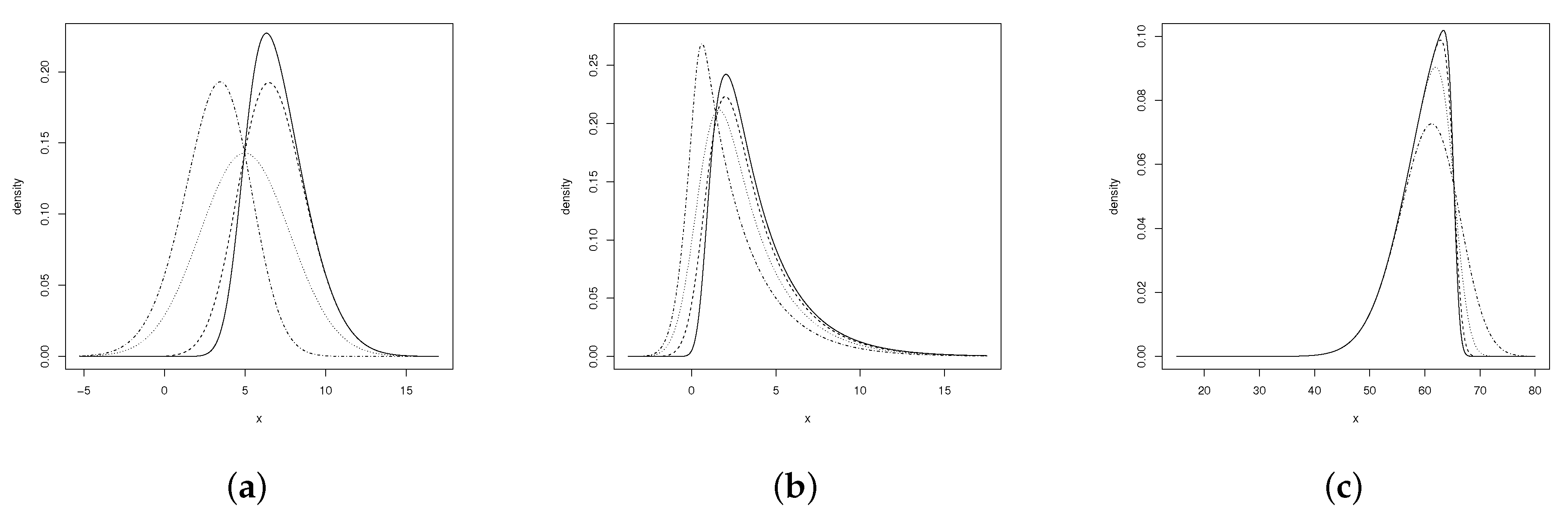
Figure 1 shows the ESN’s density behaviour for certain parameter values; (a) and (b) present a comparison between the ESN and EG distributions (the EG ensues when ESN has $\alpha =0$); (c) illustrates the case of negatively skewed ESN distributions.

The cumulative distribution function (CDF) of a random variable with an ESN distribution does not have a closed-form expression and should be calculated using a numerical approximation algorithm. It is given by:

$$F_{ESN}\left(x\right)=\frac{2}{\tau }{e}^{\frac{{}^{{\sigma }^2}}{2{\tau }^2}}A\left(x\right)$$

(8)

where:

$$A\left(x\right)={\int }_{-\infty }^x{e}^{\frac{t-\mu }{\sigma }}{\Phi }_B\left(\frac{t-\mu }{\sigma }-\frac{\sigma }{\tau },\frac{\sigma \delta }{\tau };-\delta \right)dt.$$

Moreover, the survival, hazard, and inverse risk functions are given by:

$$S_{ESN}\left(t\right)=1-\frac{2}{\tau }{e}^{\frac{{}^{{\sigma }^2}}{2{\tau }^2}}A\left(t\right),r\left(t\right)=\frac{e^{\frac{t-\mu }{\sigma }}{\Phi }_B\left(\frac{t-\mu }{\sigma }-\frac{\sigma }{\tau },\frac{\sigma \delta }{\tau };-\delta \right)}{\frac{\tau }{2}{e}^{-\frac{{\sigma }^2}{2{\tau }^2}}+A\left(t\right)},h\left(t\right)=\frac{e^{\frac{t-\mu }{\sigma }}{\Phi }_B\left(\frac{t-\mu }{\sigma }-\frac{\sigma }{\tau },\frac{\sigma \delta }{\tau };-\delta \right)}{A\left(t\right)}.$$

2.1. Moments

The moments of the ESN distribution can be obtained directly from the stochastic representation of the random variable $X=X_1+X_2\sim ESN(\tau ,\mu ,\sigma ,\alpha ),$ where $X_1\sim Exp\left(\tau \right)$ and $X_2\sim SN(\mu ,\sigma ,\alpha )$ are independent random variables. Thus, the r^th moment of the random variable $X=X_1+X_2$ is given by:

$$\begin{array}{c}\hfill \mathbb{E}\left(X^r\right)={(X_1+X_2)}^r=\sum _{j=0}^r\left(\genfrac{}{}{0pt}{}{r}{j}\right)\mathbb{E}\left(X_1^{r-j}{X}_2^j\right)=\sum _{j=0}^r\left(\genfrac{}{}{0pt}{}{r}{j}\right)\mathbb{E}\left(X_1^{r-j}\right)\mathbb{E}\left(X_2^j\right).\end{array}$$

(9)

Given that $\mathbb{E}\left(X_1^{r-j}\right)=(r-j)!$, the even moments of the SN distribution match those of the normal distribution and by expressing the odd moments of the SN distribution (see [11]), it results that:

$$\begin{array}{c}\hfill \mathbb{E}\left(X^r\right)=\sum _{j=0}^r\sum _{l=0}^j\left(\genfrac{}{}{0pt}{}{r}{j}\right)\left(\genfrac{}{}{0pt}{}{j}{l}\right)(r-j)!{\tau }^{r-j}{\mu }^{j-l}{\sigma }^l\mathbb{E}\left(Z^l\right)\end{array}$$

(10)

where:

$$\mathbb{E}\left(Z^l\right)=\left\{\begin{array}{cc}\frac{1}{\sqrt{2\pi }}{2}^{k+\frac{1}{2}}\Gamma \left(k+\frac{1}{2}\right)\hfill & \mathrm{if}l=2k,withk\in \mathbb{Z}\cup \left\{0\right\},\hfill \\ \sqrt{\frac{2}{\pi }}\alpha {(1+{\alpha }^2)}^{-\left(k+\frac{1}{2}\right)}{2}^{-k}(2k+1)!\sum _{t=0}^k\frac{t!{\left(2\alpha \right)}^{2t}}{(2t+1)!(k-t)!},\hfill & \mathrm{if}l=2k+1,withk\in \mathbb{Z}\cup \left\{0\right\}.\hfill \end{array}\right.$$

Hence, from the central moments given by $\mathbb{E}{(X-\mathbb{E}\left(X\right))}^r$, the expected value and variance of the ESN random variable are:

$$\mathbb{E}\left(X\right)=\tau +\mu +\sqrt{\frac{2}{\pi }}\sigma \delta ,Var\left(X\right)=\mathbb{E}\left(X^2\right)-{\mathbb{E}}^2\left(X\right)={\tau }^2+\left(1-\frac{2}{\pi }{\delta }^2\right){\sigma }^2,$$

(11)

Grushka [12] found that the asymmetry and kurtosis coefficients of the EG random variable depended on the scale parameters of the convolution distributions, i.e., $\tau$ and $\sigma .$ As for the ESN model, the asymmetry ($skew$) and kurtosis ($kurt$) coefficients are given by the following expressions:

$$skew=\frac{2{\left(\frac{\tau }{\sigma }\right)}^3+{\left(\frac{2}{\pi }\right)}^{3/2}\left(2-\frac{\pi }{2}\right){\delta }^3}{{\left({\left(\frac{\tau }{\sigma }\right)}^2+\left(1-\frac{2}{\pi }{\delta }^2\right)\right)}^{3/2}}$$

and:

$$kurt=\frac{3\left(3{\left(\frac{\tau }{\sigma }\right)}^4+2{\left(\frac{\tau }{\sigma }\right)}^2\left(1-\frac{2}{\pi }{\delta }^2\right)\right)+2{\left(\frac{2}{\pi }\right)}^2(\pi -3){\delta }^4}{{\left({\left(\frac{\tau }{\sigma }\right)}^2+\left(1-\frac{2}{\pi }{\delta }^2\right)\right)}^2}.$$

where $\delta =\frac{\alpha }{\sqrt{1+{\alpha }^2}}$ and $sgn(·)$ denotes the sign function. Therefore, in line with Grushka’s findings [12], ($skew$) and ($kurt$)depend on $\frac{\tau }{\sigma }$ and the asymmetry parameter $\alpha .$

A $(0,\infty )\times (-1000,1000)$ grid is constructed for $\frac{\tau }{\sigma }\in (0,\infty )$ and $\alpha \in (-1000,1000)$ values and $skew$ values within $(-0.995267,1.99999)$; these values are obtained numerically using R statistical software. Doing so indicated that if $\frac{\tau }{\sigma }\to \infty ;\alpha \to \pm \infty$, then $skew\to 2$; while if $\frac{\tau }{\sigma }\to 0;\alpha \to \infty$, then $skew\to 0.9953.$ Moreover, if $\frac{\tau }{\sigma }\to 0;\alpha \to -\infty$, then $skew\to -0.9953$; and if $\frac{\tau }{\sigma }\to 0;\alpha \to 0$, then $skew\to 0.$ Therefore, the range of asymmetry of the ESN model is (−0.9953, 2], which makes it more flexible than the EG model and other asymmetric models such as the SN model [9] and the power-normal model [13,14].

Similarly, for the same range of $\frac{\tau }{\sigma }$ and $\alpha$ values, the kurtosis coefficient is within the $(0.006039,8.99999)$ range (these values were obtained numerically using the R statistical software). Moreover, if $\frac{\tau }{\sigma }\to \infty ;\alpha \to \pm \infty$, then $kurt\to 9$; while if $\frac{\tau }{\sigma }\to 0;\alpha \to \pm \infty$, then $kurt\to 0.8692$, and if $\frac{\tau }{\sigma }\to 0;\alpha \to 0$, then $kurt\to 0.$ Therefore, the kurtosis range of the ESN model makes the ESN more flexible than asymmetric models, including the SN model [9], the power-normal model [13,14] and the SN Alpha-power model [15].

The moment- and characteristic-generating functions of the ESN model are given by:

$$M_X\left(t\right)=2e^{\mu t+\frac{1}{2}{\sigma }^2{t}^2}{\left(1-\frac{t}{\tau }\right)}^{-1}\Phi \left(\sigma \delta t\right)$$

and:

$${\varphi }_c\left(t\right)=2e^{it\mu -\frac{1}{2}{\sigma }^2{t}^2}{\left(1-\frac{it}{\tau }\right)}^{-1}\Phi \left(\sigma \delta it\right).$$

Note that, for $a\in \mathbb{R}$ and $b>0,$

$$M_{a+bX}\left(t\right)=2e^{(\mu +a)t+\frac{1}{2}{\left(b\sigma \right)}^2{t}^2}{\left(1-\frac{t}{\tau /b}\right)}^{-1}\Phi \left(\left(b\sigma \right)\delta t\right),$$

which means that $a+bX\sim ESN\left(\tau /b,a+\mu ,b\sigma ,\alpha \right).$ In other words, the ESN distribution is closed for the linear combination of the form $a+bX.$

2.2. Exponential-Centred Sn Distribution

The skew-normal model is a suitable alternative for datasets with a significant degree of asymmetry; however, its drawback is that it has a singular information matrix if its asymmetry parameter equals zero, i.e., $\alpha =0$ [9]. Regarding this case (in which $\alpha$ is in the proximity of zero), some authors have proposed a reparameterization [16]. Another option is to use the so-called centred skew-normal distribution [9], which is obtained as shown below.

For $Z\sim SN\left(\alpha \right),$ with $\mathbb{E}\left(Z\right)=b\delta$ and $Var\left(Z\right)=1-{\left(b\delta \right)}^2$ where $b=\sqrt{\frac{2}{\pi }}$ and $\delta =\frac{\alpha }{\sqrt{1+{\alpha }^2}}$, let the Y random variable be defined as:

$$Y=\xi +\eta \frac{Z-\mathbb{E}\left(Z\right)}{\sqrt{Var\left(Z\right)}},-\infty <\xi <\infty ,\eta >0.$$

For this random variable, it follows that:

$$\mathbb{E}\left(Y\right)=\xi \mathrm{and}Var\left(Y\right)={\eta }^2.$$

Given that the random variable Y is a linear combination of $Z\sim SN\left(\alpha \right)$, Y also follows an SN distribution, and after some calculations, it results that:

$$Y=\mu +\sigma Z\sim SN(\mu ,\sigma ,\alpha )$$

where:

$$\begin{array}{c}\hfill \mu =\xi -c\eta {\gamma }_1^{1/3},\end{array}\begin{array}{c}\hfill \sigma =\eta \sqrt{1+c^2{\gamma }_1^{2/3}},\end{array}\begin{array}{c}\hfill \alpha =\frac{c{\gamma }_1^{1/3}}{\sqrt{b^2+c^2(b^2-1){\gamma }_1^{2/3}}}\end{array}$$

(12)

with $c={\{2/(4-\pi )\}}^{1/3}$ and $-0.9953<{\gamma }_1<0.9953$ (these values are provided in [9]).

This is known as the centred SN (CSN) distribution and is denoted by $CSN(\xi ,\eta ,{\gamma }_1).$

Ref. [9] showed that the information matrix of the CSN model can be written as:

$$I\left(\mathbf{\theta }\right)=D^{T}I\left({\mathbf{\theta }}_1\right)D,$$

(13)

where $I\left({\mathbf{\theta }}_1\right)$ is the information matrix of the SN model; D the matrix of the derivatives of the parameter vector ${\mathbf{\theta }}_1=(\mu ,\sigma ,{\gamma }_1)$ with respect to the parameter vector $\mathbf{\theta }=(\xi ,\eta ,\lambda );$ [9] showed that $I\left(\mathbf{\theta }\right)$ is a non-singular matrix.

Hence, based on this very reparameterization, the exponential-centred SN model is given by:

$$\begin{array}{c}\hfill g\left(x\right)=\frac{2}{\tau }{e}^{-\frac{x-\xi +c\eta {\gamma }_1^{1/3}}{\tau }+\frac{{\eta }^2\left(1+c^2{\gamma }_1^{2/3}\right)}{2{\tau }^2}}{\Phi }_B\left(\frac{x-\xi +c\eta {\gamma }_1^{1/3}}{\eta \sqrt{1+c^2{\gamma }_1^{2/3}}}-\frac{\eta \sqrt{1+c^2{\gamma }_1^{2/3}}}{\tau },\frac{\eta {\delta }_1\sqrt{1+c^2{\gamma }_1^{2/3}}}{\tau };-{\delta }_1\right)\end{array}$$

(14)

with ${\delta }_1=\frac{\alpha }{\sqrt{1+{\alpha }^2}}$ and $\alpha$ as defined in Equation (12). This model will be denoted by $ECSN(\tau ,\xi ,\eta ,{\gamma }_1).$ When ${\gamma }_1=0$, the $EG(\tau ,\mu ,{\sigma }^2)$ model is then obtained.

Note that this centred representation of the SN model reduces the space range of the asymmetry parameter since ${\gamma }_1\in (-0.9953;0.9953)$ (see [17]).

3. Estimation

For a random sample $X_1,X_2,\cdots ,X_n$ where $X_i\sim ECSN(\tau ,\xi ,\eta ,{\gamma }_1),$ it is possible to estimate the parameters of the $ECSN(\tau ,\xi ,\eta ,{\gamma }_1)$ model by maximising the log-likelihood function:

$$\begin{array}{ccc}\hfill \ell \left(\theta \right)& =& -nlog\left(\tau \right)+\frac{n{\eta }^2\left(1+c^2{\gamma }_1^{2/3}\right)}{2{\tau }^2}-\sum _{i=1}^n\frac{x_i-\xi +c\eta {\gamma }_1^{1/3}}{\tau }\hfill \\ & & +\sum _{i=1}^{n}log\left({\Phi }_B\left(\frac{x_i-\xi +c\eta {\gamma }_1^{1/3}}{\eta \sqrt{1+c^2{\gamma }_1^{2/3}}}-\frac{\eta \sqrt{1+c^2{\gamma }_1^{2/3}}}{\tau },\frac{\eta {\delta }_1\sqrt{1+c^2{\gamma }_1^{2/3}}}{\tau };-{\delta }_1\right)\right).\hfill \end{array}$$

(15)

Another alternative could be to maximise the log-likelihood function of the parameter vector ${\theta }_1=(\tau ,\mu ,\sigma ,\alpha ),$ which is given by:

$$\ell \left({\theta }_1\right)=-nlog\left(\tau \right)+\frac{n{\sigma }^2}{2{\tau }^2}-\sum _{i=1}^n\frac{x_i-\mu }{\tau }+\sum _{i=1}^{n}log\left({\Phi }_B\left(\frac{x_i-\mu }{\sigma }-\frac{\sigma }{\tau },\frac{\sigma \delta }{\tau };-\delta \right)\right),$$

(16)

and then use the relationships defined in Equation (12) to find the estimates of vector ${\theta }_1=(\tau ,\xi ,\eta ,{\gamma }_1).$ The elements of the score function $U\left({\theta }_1\right)=\left(U\left(\tau \right),U\left(\mu \right),U\left(\sigma \right),U\left(\alpha \right)\right)$, i.e., the derivative of the log-likelihood function with respect to the parameters, are given in Appendix A.

The score equations are estimated by equating the scores to zero ($U\left({\theta }_{1j}\right)=0$). Then, the maximum likelihood estimators $(\widehat{\tau },\widehat{\mu },\widehat{\sigma },\widehat{\alpha })$ of the parameter vector $(\tau ,\mu ,\sigma ,\alpha )$ are calculated by solving the system of equations $U\left({\theta }_j\right)=0$ by means of Newton–Raphson or quasi-Newton numerical methods, among others.

The observed information matrix of the parameter vector ${\theta }_1=(\tau ,\mu ,\sigma ,\alpha )$ is defined as $\Lambda \left({\mathbf{\theta }}_1\right))=-\frac{d}{d{\theta }_1}U\left({\theta }_1\right)=\left({\Lambda }_{{\theta }_{1j}{\theta }_{1j^{\prime }}}\right)$, i.e., minus the second derivative of the log-likelihood function with respect to the parameters, provided in Appendix B.

The elements of the Fisher information matrix of vector ${\theta }_1,$$K\left({\mathbf{\theta }}_1\right)$ are given by ${\kappa }_{{\theta }_{1j}{\theta }_{1j^{\prime }}}=\mathbb{E}\left({\Lambda }_{{\theta }_{1j}{\theta }_{1j^{\prime }}}\right)$ and should be calculated numerically.

The information matrix of the ECSN model can be obtained as the relationship in Equation (13) using an appropriate matrix $B={(\partial {\theta }_1/\partial \theta )}_{4\times 4}.$

Furthermore, the observed information matrix $(\Lambda (\mathbf{\theta }\left)\right)$ and Fisher information matrix $\left(K\right(\mathbf{\theta }\left)\right)$ of this model, for the parameter vector $\theta =(\tau ,\xi ,\eta ,{\gamma }_1),$ can be written in terms of the observed and expected information matrices of the ESN model, of the parameter vector ${\theta }_1=(\tau ,\mu ,\sigma ,\alpha ),$ in the form:

$$\Lambda \left(\mathbf{\theta }\right)=B^{\prime }\Lambda \left({\mathbf{\theta }}_1\right)B\mathrm{and}K\left(\mathbf{\theta }\right)=B^{\prime }K\left({\mathbf{\theta }}_1\right)B$$

(17)

where:

$$\begin{array}{c}\hfill B=\left(\begin{array}{cc}1& {\mathbf{0}}_3^T\\ {\mathbf{0}}_3& D_{3\times 3}\end{array}\right)\end{array}$$

(18)

The elements of this matrix $D_{3\times 3}$ can be found in their general form in Azzalini and Capitanio ([17], p. 68). Note that when ${\gamma }_1\to 0$, the inferior sub-matrix of size $3\times 3$ is nonsingular and converges to a diagonal matrix $diag({\sigma }^2,{\sigma }^2/2,6)$. This event entails that the matrix $K\left(\mathbf{\theta }\right)$ is nonsingular for $0<\tau <\infty$.

Therefore, in regular conditions and by applying the asymptotic theory to the maximum likelihood estimator vector of the parameter vector $\theta ,$$\Lambda \left(\theta \right)\to K\left(\theta \right).$ Then, using the same stochastic convergence argument, it follows that $\widehat{\theta }$ converges to a normal distribution; that is:

$$\sqrt{n}(\widehat{\theta }-\theta )\stackrel{d}{\to }{N}_4(\mathbf{0},{\Delta }^{-1}\left(\theta \right)).$$

Hence, for the ECSN convolution model, the elements in the diagonal of ${\Delta }^{-1}\left(\widehat{\theta }\right)$ represent the estimates of the variances of $\widehat{\tau },\widehat{\xi },\widehat{\eta }$ and ${\widehat{\gamma }}_1$. The $100\times (1-\beta )\%$ confidence intervals can be estimated in the conventional ${\theta }_j\mp Z_{1-\beta /2}{\sigma }_{jj}$ form, where ${\sigma }_{jj}$ represents the standard error of the parameter ${\theta }_j$.

3.1. Illustrations

3.1.1. Reaction Times

Ref. [18] investigated the sensorimotor processing of words by using a masked priming (MP) task. The MP is a task commonly used in experimental psychology and in which a prime word (e.g., below) is “sandwiched” for a short time (e.g., 35 ms) between a preceding masking pattern (or forward mask, e.g., LKPFH; shown for, say, 200 ms) and a proceeding target word (e.g., above; shown until a response is made). In some variations, there can be a masking pattern between the prime and the target word (called backward mask), and this was the case in Ansorge et al.’s study (such a pattern was shown for approximately 35 ms). Traditionally, there are congruent and incongruent trials; in the former case, there is a match between the response of the participant and a correct or expected response, while in the latter, there is a mismatch between those responses. The time the participant takes in responding is known as the reaction time (RT) and is measured in milliseconds.

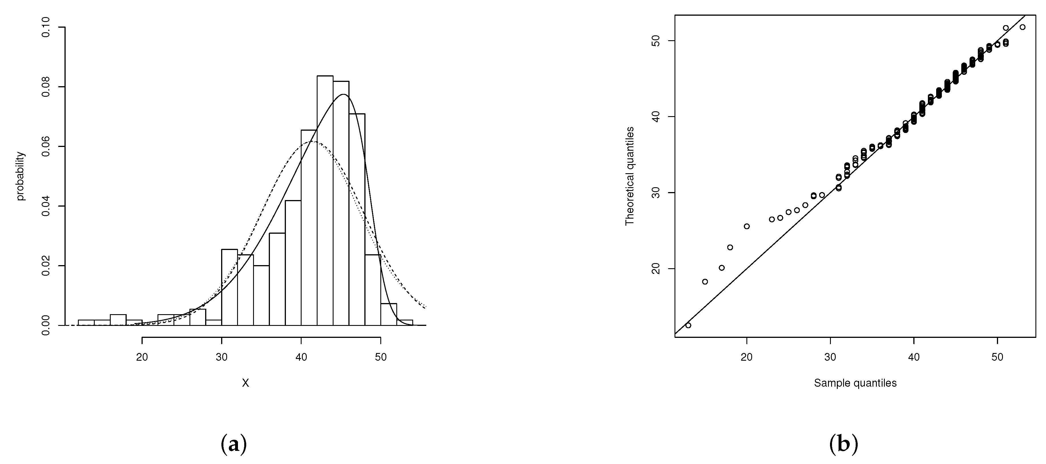
Twelve females and 12 males participated in an MP task, and their RTs were collected for both congruent and incongruent trials (see Experiment 2a). The descriptive statistics for the distribution of mean RTs during incongruent trials were as follows: $\overline{X}=890.1149$, $s=98.6875$, $b_1=-0.5326$, and $b_2=4.1798$. These statistics indicated that the distribution of RTs was negatively skewed; hence, an EG distribution would not provide an appropriate fit as its asymmetry is always positive. When the data were fitted with the ECSN, the following estimates were obtained: $\widehat{\tau }=0.2927\left(0.00002\right),$ $\widehat{\mu }=977.1546\left(0.0058\right),$ $\widehat{\sigma }=130.3170\left(0.0058\right)$ and $\widehat{\alpha }=-1.8182\left(0.0041\right)$. Considering the centred representation of the ECSN model, the estimated parameters were as follows: $\widehat{\tau }=0.2927\left(0.00002\right),$ $\widehat{\xi }=886.0465\left(0.1350\right),$ $\widehat{\nu }=93.1774\left(0.1319\right)$ and $\widehat{\gamma }=-0.4012\left(0.0034\right)$. Therefore, the ECSN gave an optimal fit, and it was further corroborated via the Kolmogorov–Smirnov (D) test; $D=0.16667$, $p-\mathrm{value}=0.9024$ (in this work, the D test is used to assess the suitability of a given statistical distribution to a dataset. However, other tests exist; e.g., Cramér–von Mises, Anderson–Darling, Shapiro–Wilk, ${\chi }^2$, Hosmer–Lemeshow, Kuiper, Kernelized Stein discrepancy, Moran, and Zhang’s $Z_K$, $Z_C$ and $Z_A$ tests). Figure 2 displays the distribution of mean RTs and the ECSN distribution’s fits.

The following example is provided to illustrate that negatively skewed data can emerge in situations other than RTs. For example, in psychometrics, some rating scales can show a negative skew.

3.1.2. The Flourishing Scale

Ref. [19] validated the Flourishing Scale (FS) in a sample of adults ($n=275$) with low and moderate levels of well-being. The FS rating scale is an eight item measure of social-psychological functioning that tackles aspects such as relationships, self-esteem, purpose and optimism.

The authors aimed to understand the distribution of the total Flourishing scores (X = TFS, $X\in {\mathbb{Z}}^{+}$); a global measure of the core aspects of individuals’ optimal social and psychological functioning. The descriptive statistics of the TFS showed an average of $\overline{X}=41.44,$ a standard deviation of $s=6.48,$ a skewness of $skew=-1.4394$ and a kurtosis of $kurt=5.8725$. The negative skewness suggested that the EG model was not the most suitable option because its range of asymmetry was positive. In addition, the high kurtosis left little room for models such as the SN, whose ranges of kurtosis and asymmetry were [3, 3.86) and (−0.9953, 0.9953), respectively.

The EG, the skew-normal Alpha-power (SNAP) and the ECSN models were fitted to the data. The exponential representation $\tau exp(-\tau x)$ was used for those models. The four parameter model $SNAP(\mu ,\sigma ,\lambda ,\alpha )$, studied by [15], is more flexible than its SN and power-normal (PN) counterparts because when $\alpha =1$, the SN distribution was obtained, and when $\lambda =0$, the PN distribution was obtained; a normal distribution ensues when $\lambda =0$ and $\alpha =1$. The SNAP’s ranges of asymmetry and kurtosis were $[-1.4676,0.9953)$ and $[1.4672,5.4386],$ respectively [15], which made it a good fit to the TFS data.

These models were compared using the Akaike information criterion (AIC) [20] and the Bayesian information criterion (BIC) of Schwarz [21], defined as:

$$AIC=-2\ell \left(\theta \right)+2p\mathrm{and}BIC=-2\ell \left(\theta \right)+plog\left(n\right)$$

where p is the number of parameters of the vector $\theta$ of the specific model. Based on the results of the AIC and the BIC, the most suitable model for the TFS data was the ECSN model (see

Table 1. MLE parameter estimates (with standard errors in parentheses) of the EG, SNAP, and ECSN models. The estimates of the ECSN model correspond to the centred model.

Parameter	EG Model		SNAP Model		ECSN Model
	Estimate		Estimate		Estimate
$\widehat{\xi }$	41.0257(0.7945)		46.1732(1.3908)		41.0952(0.4073)
$\widehat{\eta }$	6.4577(0.2783)		6.8396(2.0609)		5.8089(0.5621)
$\widehat{\tau }$	2.4131(4.0354)		2.4579(0.1903)		3.7056(0.0037)
$\widehat{\gamma }$			0.1226(0.0350)		−0.8642(0.4082)
AIC	1813.33		1817.23		1739.91
BIC	1824.18		1831.69		1754.37

). Figure 3 further shows the good fit of the ECSN model. Figure 4 shows the low degree of fit of the EG (a) and the SNAP (b) models; but it is evident that the EG gave a better fit than SNAP (see also the AIC and BIC values in Table 1).

A null hypothesis test of no difference between the ECSN model and the EG model can be expressed as,

$$H_{01}:\alpha =0\mathrm{versus}{H}_{11}:\alpha \ne 0.$$

By using the likelihood-ratio test (models are nested),

$${\Lambda }_1=\frac{L_{EG}\left(\widehat{\mathbf{\theta }}\right)}{L_{ECSN}\left(\widehat{\mathbf{\theta }}\right)}.$$

it is found that:

$$-2log\left({\Lambda }_1\right)=-2(-903.665+865.955)=75.4198,$$

This was a value larger than the critical 5% chi-squared value, i.e., ${\chi }_{1,95\%}^2=3.8414.$ Therefore, the null hypothesis was rejected, and it could be concluded that the ECSN model—which involved one extra parameter, making it more flexible in terms of asymmetry—fit the data better than the EG model (compare Figure 3b and Figure 4a).

Furthermore, the D test was used to determine the best fit for the TFS data. The results were as follows: for the EG model, D = 0.200 (p-value = 0.000); for the SNAP model, D = 0.2290 (p-value = 0.000); and for the ECSN model, D = 0.0981 (p-value = 0.1411). The results thus corroborated that the ECSN model was suitable for the TFS data.

4. Discussion

Data can take different distributional shapes, but some shapes are more common in certain research fields (for more information about other distributions and their applications, see the Special Issues in Volume 11 Issue 11 (year 2019) and Volume 12 Issue 5 (year 2020) in this journal). RTs, for example, are a ubiquitous metric in experimental psychology, and it is well known that their distribution is positively skewed. However, that is not necessarily always the case, and normally or negatively shaped RTs can ensue. In those cases, the EG distribution, a distribution traditionally used to model RT data, is not able to fit the data well. In this article, a distribution capable of fitting traditional RT data and RT data that deviate from a positive skew was proposed.

It is important, however, to frame the proposed distribution within the larger field of data analysis and modelling. While most research across scientific fields tends to focus on average differences, not much attention is paid to investigate group differences in variation. Indeed, tests designed to account for both location and scale (e.g., the Cucconi test) are rarely used. Adopting a distributional modelling approach enables tackling data differently by considering, at a minimum, the data’s location (e.g., mean) and scale (e.g., SD). To our knowledge, the only existing statistical approach able to model data in a proper distributional manner is the generalised additive models for location, scale and shape (GAMLSS).

To conclude, the ECSN distribution was proposed as a new statistical distribution suitable to adjust the shape of RT data. As the ECSN was a four parameter distribution, it could be used to model RT data’s location, scale and shape. It is our hope to see this distribution implemented in the GAMLSS R package so that it is put to the test in research contexts. The necessary Rcodes and datasets to reproduce the estimations and plots reported here can be found at https://figshare.com/projects/Two_new_distributions_for_the_modelling_of_RT_data/81743.

References

- Hohle, R.H. Inferred components of reaction times as functions of foreperiod duration. J. Exp. Psychol. 1965, 69, 382–386. [Google Scholar] [CrossRef]
- Tejo, M.; Niklitschek-Soto, S.; Marmolejo-Ramos, F. Fatigue-life distributions for reaction time data. Cogn. Neurodyn. 2018, 12, 351–356. [Google Scholar] [CrossRef] [PubMed]
- Tejo, M.; Araya, H.; Niklitschek-Soto, S.; Marmolejo-Ramos, F. Theoretical models of reaction times arising from simple-choice tasks. Cogn. Neurodyn. 2019, 13, 409–416. [Google Scholar] [CrossRef] [PubMed]
- Leiva, V.; Tejo, M.; Guiraud, P.; Schmachtenberg, O.; Orio, P. Modeling neural activity with cumulative damage distributions. Biol. Cybern. 2015, 109, 421–433. [Google Scholar] [CrossRef] [PubMed]
- Martínez-Flórez, G.; Barranco-Chamorro, I.; Bolfarine, H.; Gómez, H. Flexible Birnbaum–Saunders distribution. Symmetry 2019, 11, 1305. [Google Scholar] [CrossRef] [Green Version]
- Iriarte, Y.; Varela, H.; Gómez, H.; Gómez, H. A Gamma-Type distribution with applications. Symmetry 2020, 12, 870. [Google Scholar] [CrossRef]
- McGill, W.J. Stochastic latency mechanisms. In Handbook of Mathematical Psychology; Luce, R.D., Bush, R.R., Galanter, E., Eds.; Wiley: New York, NY, USA, 1963; Volume 1, pp. 309–359. [Google Scholar]
- Christie, L.S.; Luce, R.D. Decision structure and time relations in simple choice behavior. Bull. Math. Biophys. 1956, 18, 89–112. [Google Scholar] [CrossRef]
- Azzalini, A. A class of distributions which includes the normal ones. Scand. J. Stat. 1985, 12, 171–178. [Google Scholar]
- Azzalini, A.; Capitanio, A. The Skew-Normal and Related Families, 1st ed.; Cambridge University Press: Cambridge, UK, 2013. [Google Scholar]
- Ma, Y.; Genton, M.G. Flexible class of skew-symmetric distributions. Scand. J. Stat. 2004, 31, 459–468. [Google Scholar] [CrossRef] [Green Version]
- Grushka, E. Characterization of exponentially modified Gaussian peaks in chromatography. Anal. Chem. 1972, 44, 1733–1738. [Google Scholar] [CrossRef] [PubMed]
- Durrans, S.R. Distributions of fractional order statistics in hydrology. Water Resour. Res. 1992, 28, 1649–1655. [Google Scholar] [CrossRef]
- Pewsey, A.; Gómez, H.W.; Bolfarine, H. Likelihood-based inference for power distributions. Test 2012, 21, 775–789. [Google Scholar] [CrossRef]
- Martínez-Flórez, G.; Bolfarine, H.; Gómez, H. Skew-normal alpha-power model. Statistics 2014, 48, 1414–1428. [Google Scholar] [CrossRef]
- Rotnitzky, A.; Cox, D.R.; Bottai, M.; Robins, J. Likelihood-based inference with singular information matrix. Bernoulli 2000, 6, 243–284. [Google Scholar] [CrossRef]
- Azzalini, A.; Capitanio, A. Statistical Applications of the Multivariate Skew Normal Distribution. J. R. Stat. Soc. 1999, 61, 579–602. [Google Scholar] [CrossRef]
- Ansorge, U.; Kiefer, M.; Khalid, S.; Grassl, S.; König, P. Testing the theory of embodied cognition with subliminal words. Cognition 2010, 116, 303–320. [Google Scholar] [CrossRef] [PubMed]
- Schotanus-Dijkstra, M.; ten Klooster, P.; Drossaert, C.; Pieterse, M.; Bolier, L.; Walburg, J.; Bohlmeijer, E. Validation of the Flourishing Scale in a sample of people with suboptimal levels of mental well-being. BMC Psychol. 2016, 4, 12. [Google Scholar] [CrossRef] [PubMed] [Green Version]
- Akaike, H. A new look at statistical model identification. IEEE Trans. Autom. Control 1974, 19, 716–723. [Google Scholar] [CrossRef]
- Schwarz, G. Estimating the dimension of a model. Ann. Stat. 1978, 6, 461–464. [Google Scholar] [CrossRef]
Figure 1.
ESN distribution of (a) , and (dash-dotted line); (dotted line); (dashed line); and (solid line); (b) , and (dash-dotted line); (dotted line); (dashed line); and (solid line); (c) , and (dash-dotted line); (dotted line); (dashed line); and (solid line).
Figure 2.
Histogram and overlaid PDF of the distribution of mean RTs (a); RTs’ ECDF(solid line) and ECSN distribution’s CDF (dashed line) (b); and QQ-plot representing the ECSN distribution’s goodness of fit (c).
Figure 3.
(a) Histogram of the total Flourishing score (TFS) data and estimated densities (EG model (dashed line), SNAP model (dotted line) and ECSN model (solid line)); (b) QQ-plot of the ECSN model.
Figure 4.
QQ-plots and TFS data. (a) QQ-plot of the EG model; (b) QQ-plot of the SNAP model.