An Improved Fast Affine Motion Estimation Based on Edge Detection Algorithm for VVC

Abstract

As a newly proposed video coding standard, Versatile Video Coding (VVC) has adopted some revolutionary techniques compared to High Efficiency Video Coding (HEVC). The multiple-mode affine motion compensation (MM-AMC) adopted by VVC saves approximately 15%-25% Bjøntegaard Delta Bitrate (BD-BR), with an inevitable increase of encoding time. This paper gives an overview of both the 4-parameter affine motion model and the 6-parameter affine motion model, analyzes their performances, and proposes improved algorithms according to the symmetry of iterative gradient descent for fast affine motion estimation. Finally, the proposed algorithms and symmetric MM-AMC flame of VTM-7.0 are compared. The results show that the proposed algorithms save 6.65% total encoding time on average, which saves approximately 30% encoding time of affine motion compensation.

1. Introduction

H.264/AVC [1] was successfully standardized in 2003, which can provide better quality of the reconstructed image under the same bandwidth. Soon after that, the ITU-T Video Coding Experts Group (VCEG) and ISO/IEC Moving Picture Experts Group (MPEG) set the technical performance goals for the next generation video coding standard. As the replacement of AVC, the High Efficiency Video Coding (H.265/HEVC) [2] was finalized in 2013. HEVC has been demonstrated that can save about 50% bitrate comparing to the bitrate of AVC, while the subjective qualities are approximately the same [3].

To be compatible with the transmission and broadcasting of high-definition videos in recent years, ISU and ISO are developing the Versatile Video Coding (VVC)—a new standard which is expected to be standardized by 2020 [4]. Now the works of standardization is close to the end. VVC continues to use the block-based coding structure but adopts some new methods.

In the inter-prediction process, the affine motion model was adopted as an important coding tool, saving approximately 15–25% BD-rate alone in the current test model. HEVC uses Translational Motion Compensation (TMC) as the underlying model for motion compensation, meaning that the object motion information is presented by only one motion vector. This model cannot effectively predict rotation, scale, and shearing motion in most video sequences.

Studies of affine motion compensation (AMC) have always been a subject, while many former studies have tried to embed the affine motion model into the frame of AMC [5], but the proposals had never been adopted prior to VVC. The impediments are as follows [6]: 1. The former AMC proposals introduced greatly increase complexity, which is intolerable in most cases; and 2. an elegant AMC frame is much more complicated and requires adjustment in nearly all processes of inter-prediction.

To adaptively choose different affine motion models, Qualcomm’s response to the CFP proposed the multiple model affine motion compensation (MM-AMC) and efficient MVPs for AMC [7]. The proposed MM-AMC and efficient MVPs for AMC were adopted into VVC in July 2018. Based on this foundation, this paper proposes improved methods, and the rest of the paper is organized as follows:

In Section 2, a description of AMC in VVC is presented. Section 3 analyzes the performance of the AMC and proposes improved algorithms. The experimental procedure and results are shown in Section 4. Finally, the paper is concluded in Section 5.

2. Related Works

The affine motion model is based on the theory of affine transformations (also called affine mapping), which consists of a linear transformation followed by a translation transformation. If the changes of motion vectors meet the conditions of affine transformations, figures with any shapes (simple or complex) can be applied to the affine motion model. In the field of video coding, the affine motion model can predict some basic transformations such as rotation, zooming and translation in 2-D pictures for their transformation functions are linear.

Rotation, scale, and shearing motion exist in most video sequences and always become a more complicated motion with the combination of each other or translational motion. To linearly express those motions, V. E. Seferidis and M. Ghanbari [8] proposed higher-order motion models in 1993, since when the affine motion model has been widely employed for its simplicity.

In the block-based affine motion model, motion vectors (MVs) of each Control-point need to be coded in AMC [9]. For example, three Control-points at the corner are needed to describe the affine motion process of a rectangular block precisely, while the parameters are three times as many as the translational motion model’s parameters.

Researchers thus recently proposed a more simplified but less accurate affine motion model [10], which only needs two Control-points’ information.

2.1. Affine Motion Model

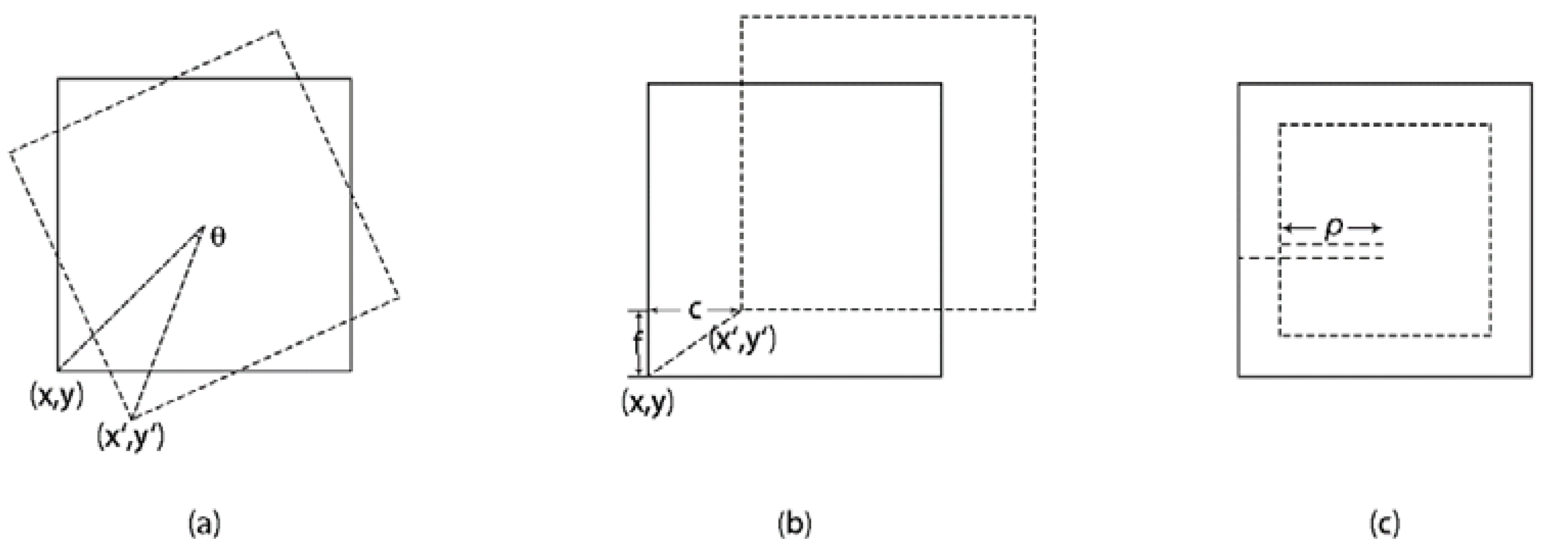
(1) 4-parameter affine motion model: The 4-parmeter affine motion model assumes a simplified affine motion model combining translation, rotation and zooming. Figure 1 shows these three typical motions:

Separately, two parameters (c and f) are used to describe translation, one parameter (θ) is used to describe rotation, and one parameter ($\mathsf{\rho }$) to describe zooming. These four parameters are independent, and the simplified affine motion model can be described as:

$$\{\begin{array}{c}{\mathrm{x}}^{\prime }=\mathsf{\rho }\cos \mathsf{\theta }·\mathrm{x}+\mathsf{\rho }\sin \mathsf{\theta }·\mathrm{y}+\mathrm{c}\\ {\mathrm{y}}^{\prime }=-\mathsf{\rho }\sin \mathsf{\theta }·\mathrm{x}+\mathsf{\rho }\cos \mathsf{\theta }·\mathrm{y}+\mathrm{f}\end{array}$$

(1)

where $\mathsf{\rho }$ is zooming factor, θ is rotation angle, and c and f are displacements in x and y directions. Replacing ρ cos θ and ρ sin θ with (1 + a) and b can obtain a concise expression of MVs.

$$\{\begin{array}{c}{\mathrm{mv}}^{\mathrm{h}}\left(\mathrm{x},\mathrm{y}\right)={\mathrm{x}}^{\prime }-\mathrm{x}=\mathrm{ax}+\mathrm{by}+\mathrm{c}\\ {\mathrm{mv}}^{\mathrm{v}}\left(\mathrm{x},\mathrm{y}\right)={\mathrm{y}}^{\prime }-\mathrm{y}=-\mathrm{bx}+\mathrm{ay}+\mathrm{f}\end{array}$$

(2)

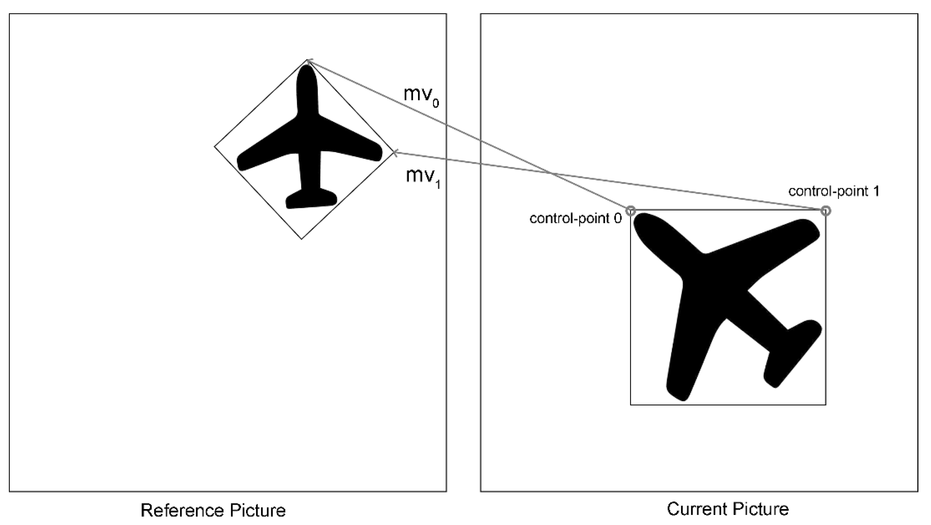
where ${\mathrm{mv}}^{\mathrm{h}}\left(\mathrm{x},\mathrm{y}\right)$ and ${\mathrm{mv}}^{\mathrm{v}}\left(\mathrm{x},\mathrm{y}\right)$ are horizontal and vertical MVs determined by a, b, c and f. Figure 2 shows an example of the 4-parameter affine motion model with two Control-points in inter-prediction.

The MVs at the top-left and top-right locations of the current block in Figure 2 are Control-point 0 and Control-point 1. The MV of any arbitrary point (x, y) can be calculated by Control-point 0 and Control-point 1.

$$\{\begin{array}{c}{\mathrm{mv}}^{\mathrm{h}}\left(\mathrm{x},\mathrm{y}\right)={\mathrm{x}}^{\prime }-\mathrm{x}=\frac{{(\mathrm{mv}}_1^{\mathrm{h}}{-\mathrm{mv}}_0^{\mathrm{h}})}{\mathrm{w}-1}\mathrm{x}-\frac{{(\mathrm{mv}}_1^{\mathrm{v}}{-\mathrm{mv}}_0^{\mathrm{v}})}{\mathrm{w}-1}{\mathrm{y}+\mathrm{mv}}_0^{\mathrm{h}}\\ {\mathrm{mv}}^{\mathrm{v}}\left(\mathrm{x},\mathrm{y}\right)={\mathrm{y}}^{\prime }-\mathrm{y}=\frac{{(\mathrm{mv}}_1^{\mathrm{v}}{-\mathrm{mv}}_0^{\mathrm{v}})}{\mathrm{w}-1}\mathrm{x}+\frac{{(\mathrm{mv}}_1^{\mathrm{h}}{-\mathrm{mv}}_0^{\mathrm{h}})}{\mathrm{w}-1}{\mathrm{y}+\mathrm{mv}}_0^{\mathrm{v}}\end{array}$$

(3)

where w is the width of the block, thus (w-1) is the distance between Control-point 0 and Control-point 1, and${\mathrm{mv}}_0^{\mathrm{h}}{,\mathrm{mv}}_0^{\mathrm{v}}{,\mathrm{mv}}_1^{\mathrm{h}}$ and ${\mathrm{mv}}_1^{\mathrm{v}}$ are the MV components of Control-point 0 and Control-point 1 in the x and y directions. The results of the four parameters (a, b, c, f) are delivered only by ${\mathrm{mv}}_0$ and ${\mathrm{mv}}_1$.

Formula (3) can also be rewritten in the form of a matrix:

$$\mathrm{mv}\left(\mathrm{x},\mathrm{y}\right)=\mathrm{A}\left(\mathrm{x},\mathrm{y}\right)·{\mathrm{MV}}_{\mathrm{A}}^{\mathrm{T}}$$

(4)

$$\mathrm{A}\left(\mathrm{x},\mathrm{y}\right)=\left[\begin{array}{cccc}(1-\frac{\mathrm{x}}{\mathrm{w}-1})& \frac{\mathrm{x}}{\mathrm{w}-1}& \frac{\mathrm{y}}{\mathrm{w}-1}& -\frac{\mathrm{y}}{\mathrm{w}-1}\\ -\frac{\mathrm{y}}{\mathrm{w}-1}& \frac{\mathrm{y}}{\mathrm{w}-1}& (1-\frac{\mathrm{x}}{\mathrm{w}-1})& \frac{\mathrm{x}}{\mathrm{w}-1}\end{array}\right]$$

(5)

$${\mathrm{MV}}_{\mathrm{A}}=[\begin{array}{cc}\begin{array}{cc}{\mathrm{mv}}_0^{\mathrm{h}}& {\mathrm{mv}}_1^{\mathrm{h}}\end{array}& \begin{array}{cc}{\mathrm{mv}}_0^{\mathrm{v}}& {\mathrm{mv}}_1^{\mathrm{v}}\end{array}\end{array}]$$

(6)

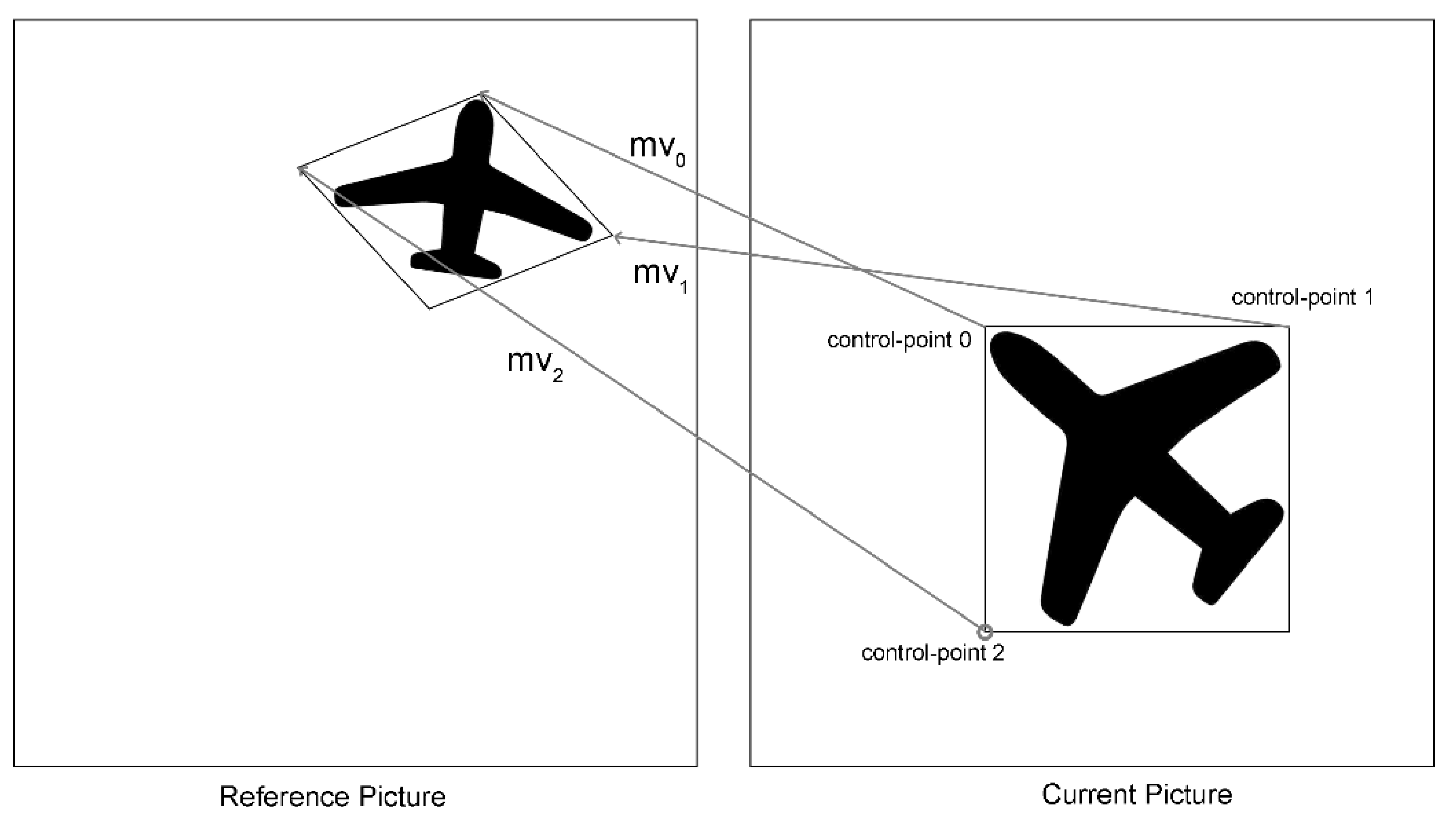
(2) 6-parameter affine motion model: The 6-parameter affine motion model can precisely predict affine motion, but needs two more parameters than the 4-parameter affine motion model.

$$\{\begin{array}{c}{\mathrm{x}}^{\prime }=\mathrm{ax}+\mathrm{by}+\mathrm{c}\\ {\mathrm{y}}^{\prime }=\mathrm{dx}+\mathrm{ey}+\mathrm{f}\end{array}$$

(7)

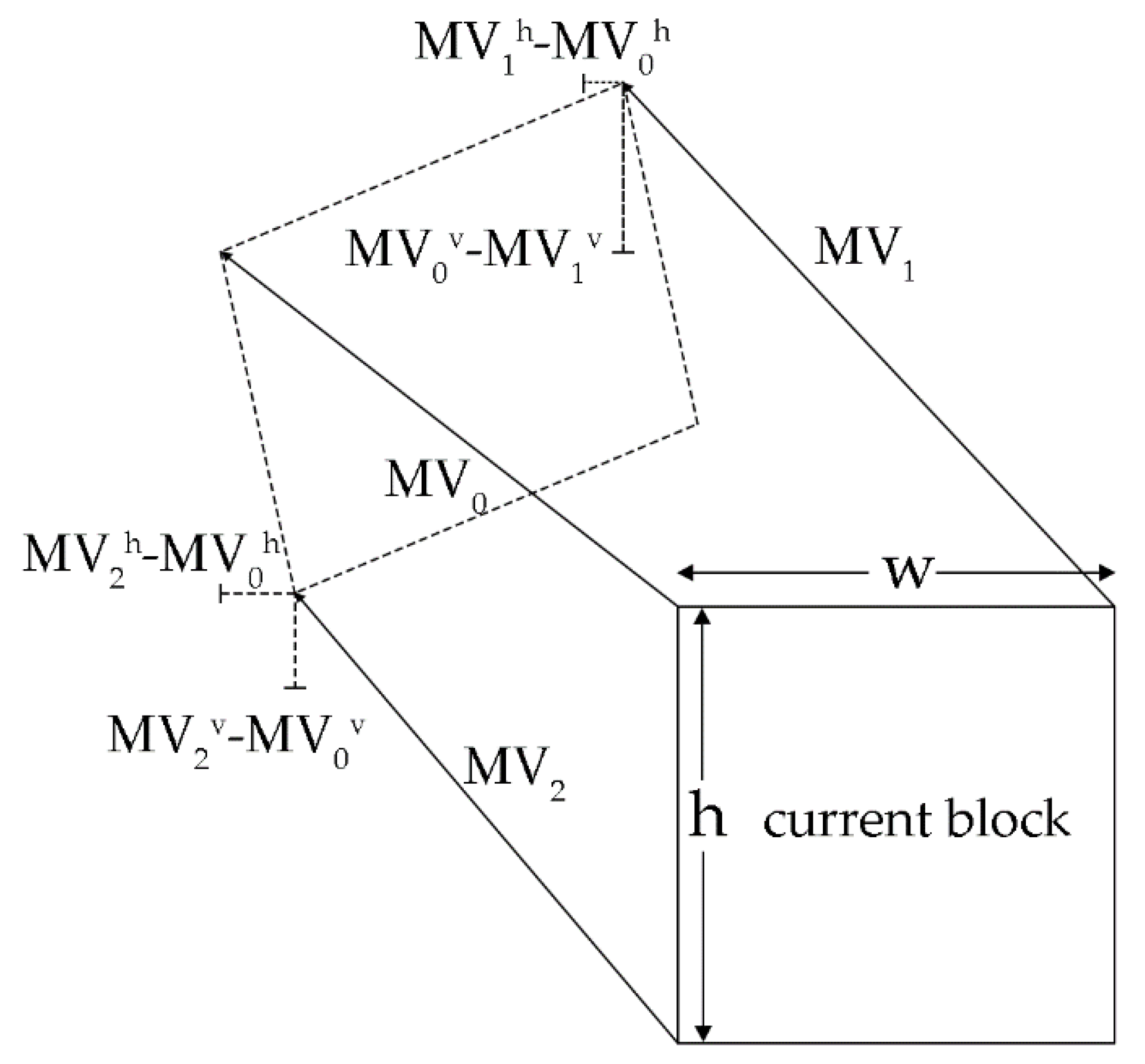
Figure 3 shows an example of the 6-parameter affine motion model with three Control-points in inter-prediction.

Control-point 2 also joins prediction. Therefore, the parameters $\mathrm{b}$ and e in Formula (7) are calculated by Control-point 0 and Control-point 2 as follows.

$$\{\begin{array}{c}{\mathrm{mv}}^{\mathrm{h}}\left(\mathrm{x},\mathrm{y}\right)=\frac{{(\mathrm{mv}}_1^{\mathrm{h}}{-\mathrm{mv}}_0^{\mathrm{h}})}{\mathrm{w}-1}\mathrm{x}+\frac{{(\mathrm{mv}}_2^{\mathrm{h}}{-\mathrm{mv}}_0^{\mathrm{h}})}{\mathrm{h}-1}{\mathrm{y}+\mathrm{mv}}_0^{\mathrm{h}}\\ {\mathrm{mv}}^{\mathrm{v}}\left(\mathrm{x},\mathrm{y}\right)=\frac{{(\mathrm{mv}}_1^{\mathrm{v}}{-\mathrm{mv}}_0^{\mathrm{v}})}{\mathrm{w}-1}\mathrm{x}+\frac{{(\mathrm{mv}}_2^{\mathrm{v}}{-\mathrm{mv}}_0^{\mathrm{v}})}{\mathrm{h}-1}{\mathrm{y}+\mathrm{mv}}_0^{\mathrm{v}}\end{array}$$

(8)

where ${\mathrm{mv}}_2^{\mathrm{h}}$ and ${\mathrm{mv}}_2^{\mathrm{v}}$ are the MV components of Control-point 2 in the x and y direction, $\mathrm{h}$ is the height of the block, and $\mathrm{h}-1$ is the distance between Control-point 0 and Control-point 2. Additionally, this formula can be rewritten as:

$$\mathrm{mv}\left(\mathrm{x},\mathrm{y}\right)=\mathrm{A}\left(\mathrm{x},\mathrm{y}\right)·{\mathrm{MV}}_{\mathrm{A}}^{\mathrm{T}}$$

(9)

$$\mathrm{A}\left(\mathrm{x},\mathrm{y}\right)=\left[\begin{array}{cc}\begin{array}{ccc}1-\frac{\mathrm{x}}{\mathrm{w}-1}-\frac{\mathrm{y}}{\mathrm{h}-1}& \frac{\mathrm{x}}{\mathrm{w}-1}& \frac{\mathrm{y}}{\mathrm{h}-1}\end{array}& \begin{array}{ccc}0& 0& 0\end{array}\\ \begin{array}{ccc}0& 0& 0\end{array}& \begin{array}{ccc}1-\frac{\mathrm{x}}{\mathrm{w}-1}-\frac{\mathrm{y}}{\mathrm{h}-1}& \frac{\mathrm{x}}{\mathrm{w}-1}& \frac{\mathrm{y}}{\mathrm{h}-1}\end{array}\end{array}\right]$$

(10)

$${\mathrm{MV}}_{\mathrm{A}}=[\begin{array}{cc}\begin{array}{ccc}{\mathrm{mv}}_0^{\mathrm{h}}& {\mathrm{mv}}_1^{\mathrm{h}}& {\mathrm{mv}}_2^{\mathrm{h}}\end{array}& \begin{array}{ccc}{\mathrm{mv}}_0^{\mathrm{v}}& {\mathrm{mv}}_1^{\mathrm{v}}& {\mathrm{mv}}_2^{\mathrm{v}}\end{array}\end{array}]$$

(11)

The 6-parameter affine motion model takes a bigger matrix to restore motion information, but half of the elements are zero value, which reduces the computing efficiency of the inter search process.

2.2. AMC

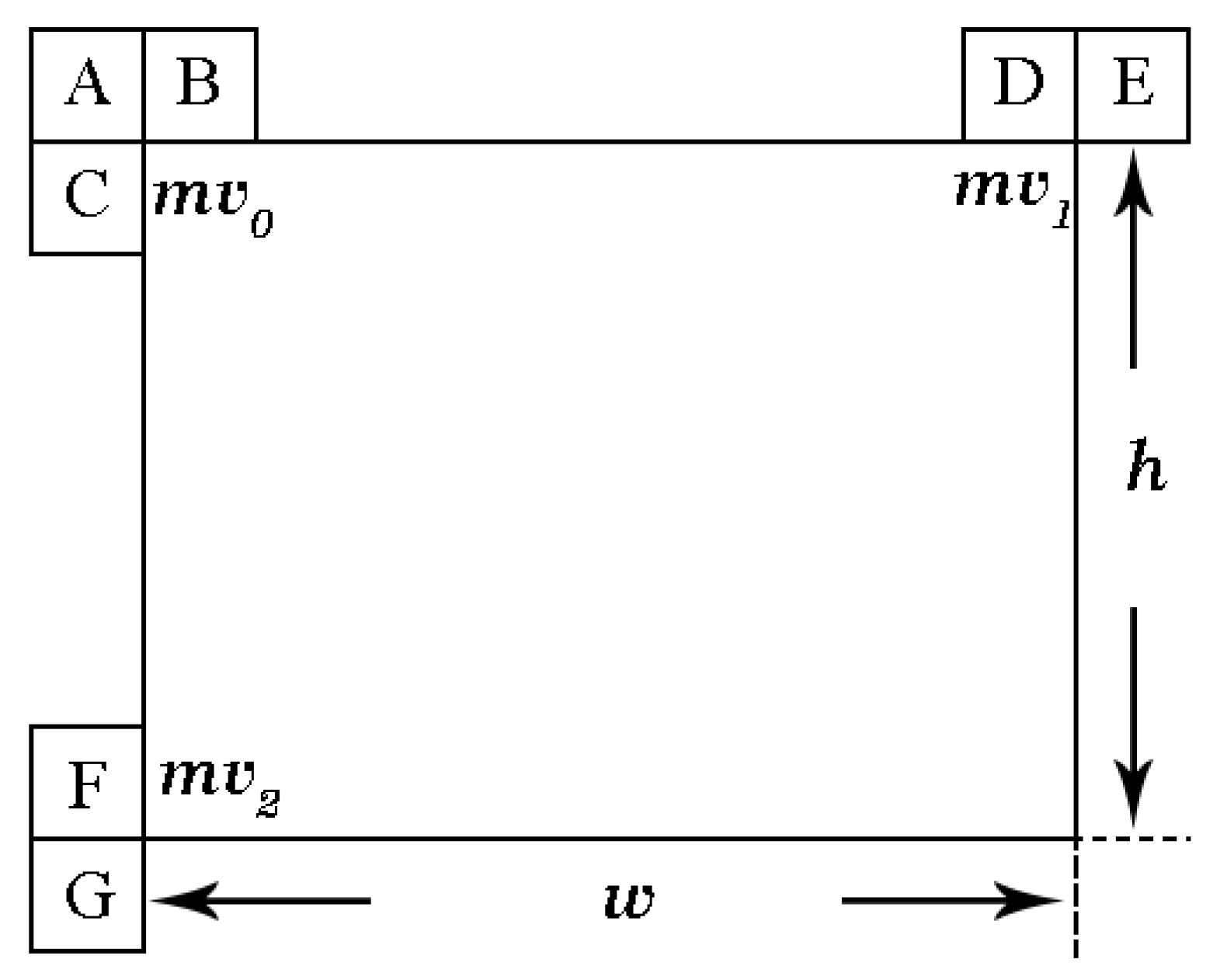
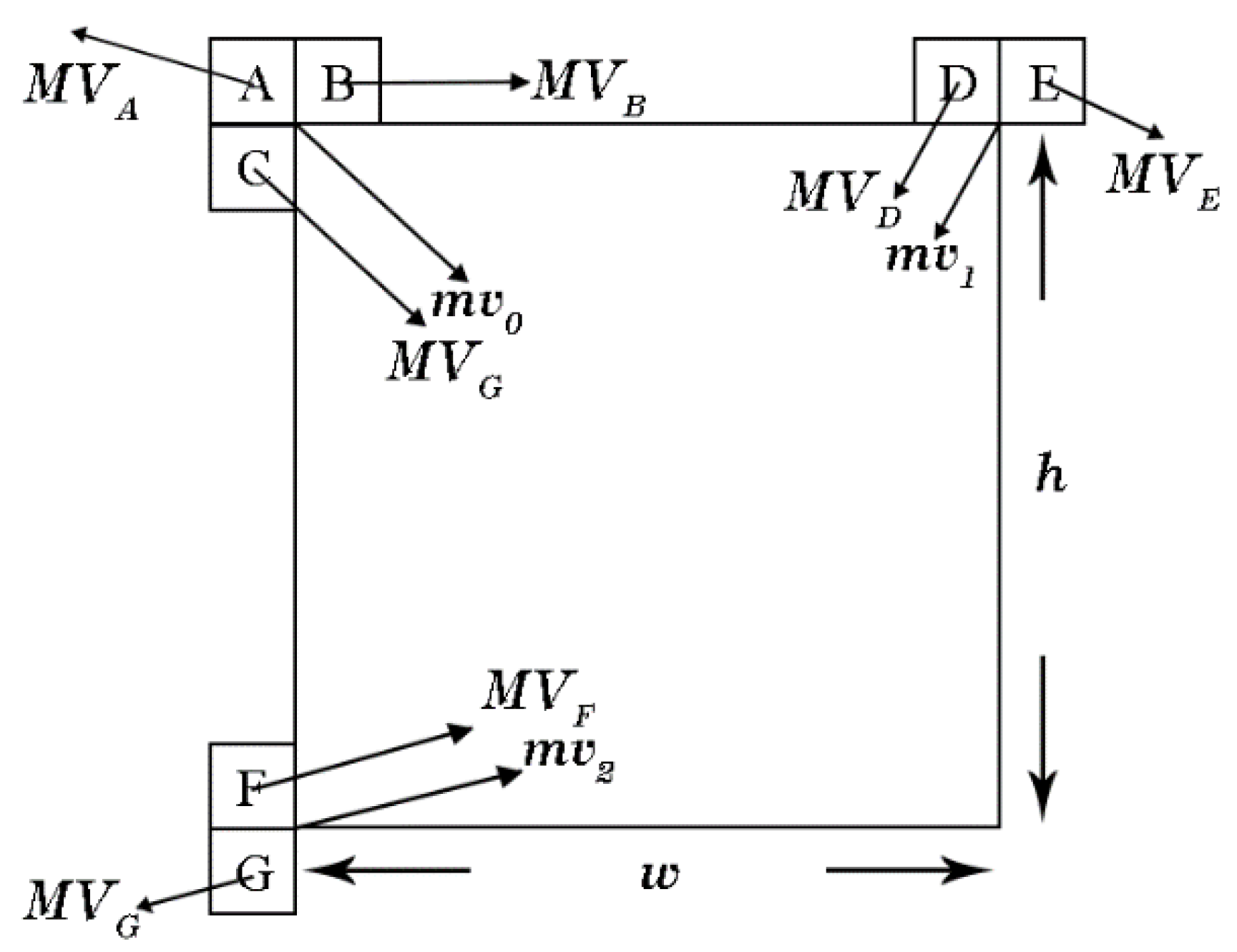
(1) Motion vector prediction(MVP): The MVP candidate list for affine inter-mode restores neighboring blocks’ MVs for the current block. To increase the robustness and consistency of the VVC encoder, the translational motion will be set as the MV tuples to fill the MVP candidate list only when the number of available MV tuples is less than the list’s length [11]. Figure 4 shows the candidate list for advanced motion vector prediction (AMVP):

There are seven MVP candidates for affine MV prediction, located at the top-left, top-right and bottom-left, and these can be categorized into three tuples.

$$\{\begin{array}{c}{\mathrm{S}}_0=\left\{{\mathrm{MV}}_{\mathrm{A}}{,\mathrm{MV}}_{\mathrm{B}}{,\mathrm{MV}}_{\mathrm{C}}\right\}\\ {\mathrm{S}}_1=\left\{{\mathrm{MV}}_{\mathrm{D}}{,\mathrm{MV}}_{\mathrm{E}}\right\}\\ {\mathrm{S}}_2{=\text{{}\mathrm{MV}}_{\mathrm{F}}{,\mathrm{MV}}_{\mathrm{G}}\text{}}\end{array}$$

(12)

where the MVs belonging to ${\mathrm{S}}_0$ are used to predict ${\mathrm{mv}}_0$, the MVs belonging to ${\mathrm{S}}_1$ are used to predict ${\mathrm{mv}}_1$ and the MVs belonging to ${\mathrm{S}}_2$ are used to predict ${\mathrm{mv}}_2$.

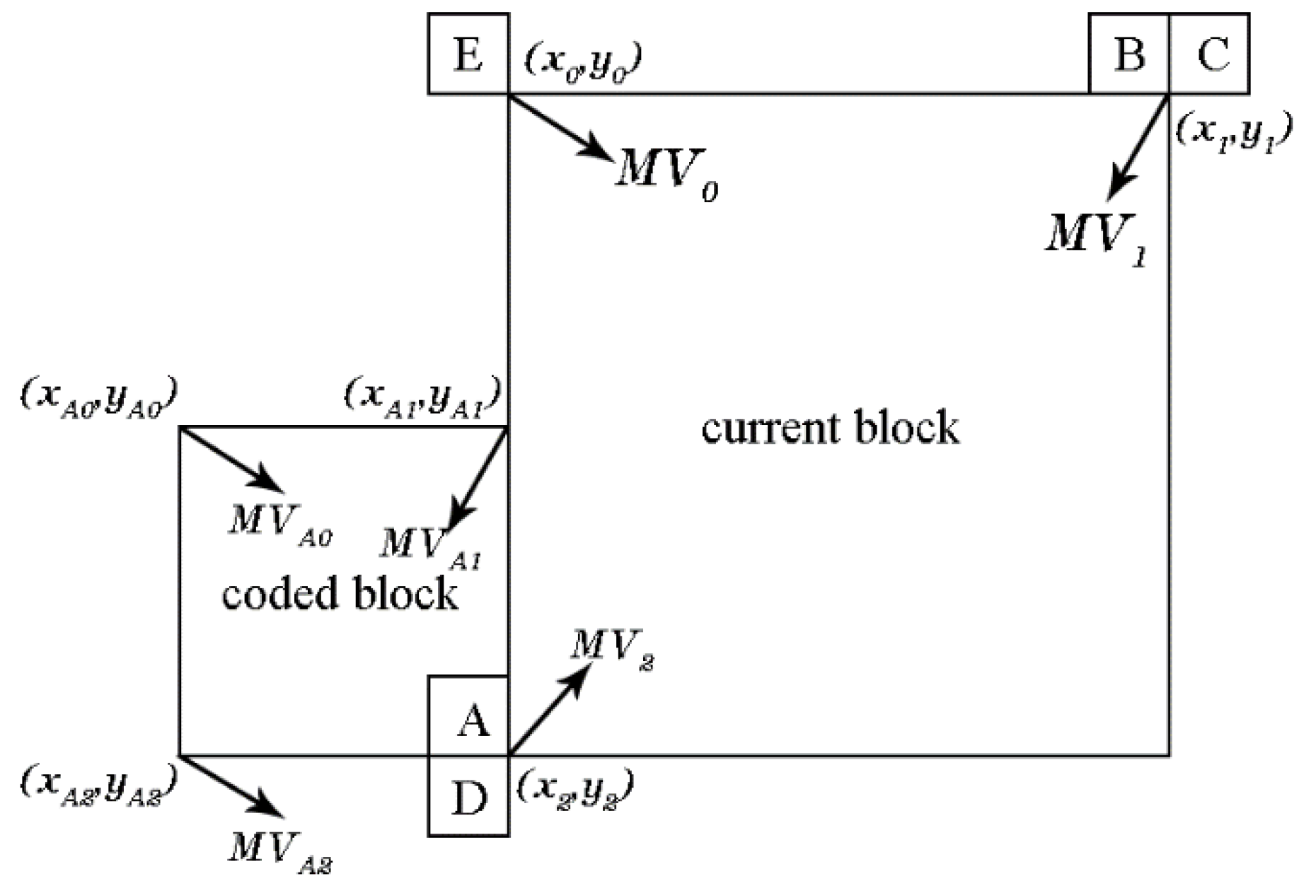
AMC provides affine advanced motion vector prediction (AAMVP) based on HEVC AMVP. As for the 4-parameter affine inter mode, ${\mathrm{mv}}_0$ and ${\mathrm{mv}}_1$ are eventually signaled explicitly to the decoder, while ${\mathrm{mv}}_2$ is used to implicitly judge the prediction correctness, and is not sent. Affine inter mode choses the best AMVP candidates of ${\mathrm{S}}_0$, ${\mathrm{S}}_1$ and motion vector difference (MVD). Therefore ${\mathrm{mv}}_0$ and ${\mathrm{mv}}_1$ can be calculated as ${\mathrm{mvp}}_0{+\mathrm{mvd}}_0$ and ${\mathrm{mvp}}_1{+\mathrm{mvd}}_1$. Figure 5 shows an example of AAMVP:

First, the encoder checks the availability of neighboring blocks (block A to G) and whether their MVs are pointing to the same reference frame as the given one.

Then the encoder side transmits all possible$\left({\mathrm{MV}}_{0,}{\mathrm{MV}}_1{,\mathrm{MV}}_2\right)$, where ${\mathrm{MV}}_{0,}\in {\mathrm{S}}_0$, ${\mathrm{MV}}_{1,}\in {\mathrm{S}}_1$ and ${\mathrm{MV}}_{2,}\in {\mathrm{S}}_2$. By setting ${\mathrm{mv}}_0={\mathrm{MV}}_0$, ${\mathrm{mv}}_1={\mathrm{MV}}_1$, the encoder predicts ${\mathrm{mv}}_2$ according to Formula (3). The smaller the difference between ${\mathrm{mv}}_2$ and ${\mathrm{MV}}_2$ is, the more probable it is that the current MV combination forms a real affine motion model. The difference value named DMV can be calculated as follows [10]:

$$\mathrm{DMV}=\left|{\mathrm{MV}}_1^{\mathrm{h}}{-\mathrm{MV}}_0^{\mathrm{h}}-\left({\mathrm{MV}}_2^{\mathrm{v}}{-\mathrm{MV}}_0^{\mathrm{v}}\right)\right|+\left|\left({\mathrm{MV}}_2^{\mathrm{h}}{-\mathrm{MV}}_0^{\mathrm{h}}\right)-\left({\mathrm{MV}}_0^{\mathrm{v}}{-\mathrm{MV}}_1^{\mathrm{v}}\right)\right|$$

(13)

Finally, the encoder explicitly transmits two $\left({\mathrm{MV}}_{0,}{\mathrm{MV}}_1\right)$ with the smallest and second-smallest DMV to the AAMVP candidate list after the traversal ends. The list will be filled with HEVC AMVP candidates if the available arrays are less than two.

(2) Fast affine motion estimation (AME) for affine inter search: HEVC uses the block-matching search algorithm for motion estimation and obtains the MV with smallest MVD [12], but the fast AME needs to calculate two or three optimal MVs simultaneously.

Usually, the encoder uses the mean square error (MSE) or the sum of absolute errors (SAD) as the matching rule. The MSE can be calculated as:

$$\mathrm{MSE}=\frac{1}{\mathrm{w}·\mathrm{h}}{\displaystyle \sum }_{\left(\mathrm{x},\mathrm{y}\right)\in \mathrm{current}\mathrm{block}}{\left|{\mathrm{Pic}}_{\mathrm{origin}}\left(\mathrm{x},\mathrm{y}\right){-\mathrm{Pic}}_{\mathrm{ref}}\left(\left(\mathrm{x},\mathrm{y}\right){+\mathrm{mv}}_{\left(\mathrm{x},\mathrm{y}\right)}\right)\right|}^2$$

(14)

where w and h are the width and height of the current block, ${\mathrm{Pic}}_{\mathrm{ref}}$ refers to the reference picture. In HEVC and VVC, encoders search the MVs through iterations, for iterative search is an efficient way to find the best MVs with the least cost. To minimize MSE, both the conventional motion estimation (CME) and the fast AME needs to find the MV close to ${\mathrm{mv}}_{\left(\mathrm{x},\mathrm{y}\right)}$ through iterations. In fact, the iteration in the process of motion estimation is a process of searching for the best MVs with the least cost. Iteration is much faster than searching every pixel and checking their costs.

Define the change of MVs at the ${\mathrm{i}}^{\mathrm{th}}$ iteration as $\mathrm{dM}{\mathrm{V}}^{\mathrm{i}}$, then the MVs at the ${\mathrm{i}}^{\mathrm{th}}$ iteration is expressed as:

$${\mathrm{mv}}_{\left(\mathrm{x},\mathrm{y}\right)}^{\mathrm{i}}=\mathrm{A}\left(\mathrm{x},\mathrm{y}\right)·{{(\mathrm{MV}}_{\mathrm{A}}^{\mathrm{i}})}^{\mathrm{T}}=\mathrm{A}(\mathrm{x},\mathrm{y})·\left({\left({\mathrm{MV}}_{\mathrm{A}}^{\mathrm{i}-1}\right)}^{\mathrm{T}}+{\left({\mathrm{dMV}}^{\mathrm{i}}\right)}^{\mathrm{T}}\right){=\mathrm{mv}}_{\left(\mathrm{x},\mathrm{y}\right)}^{\mathrm{i}-1}+\mathrm{A}(\mathrm{x},\mathrm{y})·{\left({\mathrm{dMV}}^{\mathrm{i}}\right)}^{\mathrm{T}}$$

(15)

where $\left(\mathrm{x},\mathrm{y}\right)$ is current pixel position at the ${\mathrm{i}}^{\mathrm{th}}$ iteration, and ${\mathrm{dMV}}^{\mathrm{i}+1}$ is a row matrix, whose transposed matrix is given as:

$$\begin{array}{c}{\left({\mathrm{dMV}}^{\mathrm{i}}\right)}^{\mathrm{T}}=\left[\begin{array}{c}{\mathrm{dmv}}_0^{\mathrm{h}}\\ {\mathrm{dmv}}_1^{\mathrm{h}}\\ {\mathrm{dmv}}_0^{\mathrm{v}}\\ {\mathrm{dmv}}_1^{\mathrm{v}}\end{array}\right]=\left[\begin{array}{c}{\mathrm{mv}}_0^{\mathrm{ih}}-{\mathrm{mv}}_0^{(\mathrm{i}-0)\mathrm{h}}\\ {\mathrm{mv}}_1^{\mathrm{ih}}-{\mathrm{mv}}_1^{(\mathrm{i}-1)\mathrm{h}}\\ {\mathrm{mv}}_0^{\mathrm{iv}}-{\mathrm{mv}}_0^{(\mathrm{i}-1)\mathrm{v}}\\ {\mathrm{mv}}_1^{\mathrm{iv}}-{\mathrm{mv}}_1^{(\mathrm{i}-1)\mathrm{v}}\end{array}\right],\mathrm{if}\mathrm{affine}\mathrm{model}=4\\ {\left({\mathrm{dMV}}^{\mathrm{i}}\right)}^{\mathrm{T}}=\left[\begin{array}{c}{\mathrm{dmv}}_0^{\mathrm{h}}\\ {\mathrm{dmv}}_1^{\mathrm{h}}\\ {\mathrm{dmv}}_2^{\mathrm{h}}\\ {\mathrm{dmv}}_0^{\mathrm{v}}\\ {\mathrm{dmv}}_1^{\mathrm{v}}\\ {\mathrm{dmv}}_2^{\mathrm{v}}\end{array}\right]=\left[\begin{array}{c}{\mathrm{mv}}_0^{\mathrm{ih}}-{\mathrm{mv}}_0^{(\mathrm{i}-0)\mathrm{h}}\\ {\mathrm{mv}}_1^{\mathrm{ih}}-{\mathrm{mv}}_1^{(\mathrm{i}-1)\mathrm{h}}\\ {\mathrm{mv}}_2^{\mathrm{ih}}-{\mathrm{mv}}_2^{(\mathrm{i}-1)\mathrm{h}}\\ {\mathrm{mv}}_0^{\mathrm{iv}}-{\mathrm{mv}}_0^{(\mathrm{i}-1)\mathrm{v}}\\ {\mathrm{mv}}_1^{\mathrm{iv}}-{\mathrm{mv}}_1^{(\mathrm{i}-1)\mathrm{v}}\\ {\mathrm{mv}}_2^{\mathrm{iv}}-{\mathrm{mv}}_2^{(\mathrm{i}-1)\mathrm{v}}\end{array}\right],\mathrm{if}\mathrm{affine}\mathrm{model}=6\end{array}$$

(16)

After i iterations, we have:

$${\mathrm{Pic}}_{\mathrm{ref}}\left(\left(\mathrm{x},\mathrm{y}\right){+\mathrm{mv}}_{\left(\mathrm{x},\mathrm{y}\right)}\right)={\mathrm{Pic}}_{\mathrm{ref}}\left(\left({\mathrm{x}}^{\mathrm{i}-1}{,\mathrm{y}}^{\mathrm{i}-1}\right)+\mathrm{A}\left(\mathrm{x},\mathrm{y}\right)·{\left({\mathrm{dMV}}^{\mathrm{i}}\right)}^{\mathrm{T}}\right)$$

(17)

where $\left({\mathrm{x}}^{\mathrm{i}-1}{,\mathrm{y}}^{\mathrm{i}-1}\right)$ denotes the position of reference block in last iteration. Using the Taylor’s expansion and ignoring the high-order terms, we have

$${\mathrm{Pic}}_{\mathrm{ref}}\left(\left({\mathrm{x}}^{\mathrm{i}-1}{,\mathrm{y}}^{\mathrm{i}-1}\right)+\mathrm{A}\left(\mathrm{x},\mathrm{y}\right)·{\left({\mathrm{dMV}}^{\mathrm{i}}\right)}^{\mathrm{T}}\right)\approx {\mathrm{Pic}}_{\mathrm{ref}}\left({\mathrm{x}}^{\mathrm{i}-1}{,\mathrm{y}}^{\mathrm{i}-1}\right){+\mathrm{Pic}}_{\mathrm{ref}}^{\prime }\left({\mathrm{x}}^{\mathrm{i}-1}{,\mathrm{y}}^{\mathrm{i}-1}\right)·\mathrm{A}\left(\mathrm{x},\mathrm{y}\right)·{\left({\mathrm{dMV}}^{\mathrm{i}}\right)}^{\mathrm{T}}$$

(18)

We need to find the proper value of Formula (17) that is close to the value of ${\mathrm{Pic}}_{\mathrm{origin}}\left(\mathrm{x},\mathrm{y}\right)$ in Formula (14) to minimize MSE. Therefore, by setting the relative gradients of${\mathrm{dMV}}^{\mathrm{i}}$ to zero, the maximum value can be obtained, while the ${\mathrm{dMV}}^{\mathrm{i}}$ can be solved by a simple system of linear equations.

In HEVC, the edge detection algorithm is commonly used for fast partition mode decisions [13,14]. In VVC, however, the quad tree (QT) of the HEVC coding structure is replaced by the quad-tree plus binary tree plus ternary-tree split (QT+ BT+TT) structure, and the above-mentioned methods will cause large losses in coding efficiency or can only be used in the QT structure [15].

Still, the edge detection algorithm has its uses in VVC. The VVC test model uses the Sobel operator to solve the relative gradients of${\mathrm{dMV}}^{\mathrm{i}}$ by applying convolution with the pixel matrix:

$$\{\begin{array}{c}{\mathrm{grad}}_{\mathrm{x}}=\left[\begin{array}{ccc}-1& 0& +1\\ -2& 0& +2\\ -1& 0& +1\end{array}\right]\ast \left[\begin{array}{ccc}{\mathrm{p}}_{\mathrm{x}-1,\mathrm{y}-1}& {\mathrm{p}}_{\mathrm{x}-1,\mathrm{y}}& {\mathrm{p}}_{\mathrm{x}-1,\mathrm{y}+1}\\ {\mathrm{p}}_{\mathrm{x},\mathrm{y}-1}& {\mathrm{p}}_{\mathrm{x},\mathrm{y}}& {\mathrm{p}}_{\mathrm{x},\mathrm{y}+1}\\ {\mathrm{p}}_{\mathrm{x}+1,\mathrm{y}-1}& {\mathrm{p}}_{\mathrm{x}+1,\mathrm{y}}& {\mathrm{p}}_{\mathrm{x}+1,\mathrm{y}+1}\end{array}\right]\\ {\mathrm{grad}}_{\mathrm{y}}=\left[\begin{array}{ccc}-1& -2& -1\\ 0& 0& 0\\ +1& +2& +1\end{array}\right]\ast \left[\begin{array}{ccc}{\mathrm{p}}_{\mathrm{x}-1,\mathrm{y}-1}& {\mathrm{p}}_{\mathrm{x}-1,\mathrm{y}}& {\mathrm{p}}_{\mathrm{x}-1,\mathrm{y}+1}\\ {\mathrm{p}}_{\mathrm{x},\mathrm{y}-1}& {\mathrm{p}}_{\mathrm{x},\mathrm{y}}& {\mathrm{p}}_{\mathrm{x},\mathrm{y}+1}\\ {\mathrm{p}}_{\mathrm{x}+1,\mathrm{y}-1}& {\mathrm{p}}_{\mathrm{x}+1,\mathrm{y}}& {\mathrm{p}}_{\mathrm{x}+1,\mathrm{y}+1}\end{array}\right]\end{array}$$

(19)

where ${\mathrm{grad}}_{\mathrm{x}}$ and ${\mathrm{grad}}_{\mathrm{y}}$ are the components of relative gradients on x and y directions, and ${\mathrm{p}}_{\mathrm{x},\mathrm{y}}$ is the value of pixel at $\left(\mathrm{x},\mathrm{y}\right)$. Thus, the value of ${\mathrm{Pic}}_{\mathrm{reference}}^{\prime }$ at $\left(\mathrm{x},\mathrm{y}\right)$can be calculated as:

$$\{\begin{array}{c}\frac{\partial {\mathrm{Pic}}_{\mathrm{ref}}\left(\mathrm{x},\mathrm{y}\right)}{\partial \mathrm{x}}=\left({\mathrm{P}}_{\mathrm{x}-1,\mathrm{y}+1}{+2\mathrm{P}}_{\mathrm{x},\mathrm{y}+1}{+\mathrm{P}}_{\mathrm{x}+1,\mathrm{y}+1}{-\mathrm{P}}_{\mathrm{x}+1,\mathrm{y}-1}{-2\mathrm{P}}_{\mathrm{x},\mathrm{y}-1}{-\mathrm{P}}_{\mathrm{x}-1,\mathrm{y}-1}\right)<<3\\ \frac{\partial {\mathrm{Pic}}_{\mathrm{ref}}\left(\mathrm{x},\mathrm{y}\right)}{\partial \mathrm{y}}=\left({\mathrm{P}}_{\mathrm{x}-1,\mathrm{y}+1}{+2\mathrm{P}}_{\mathrm{x}-1,\mathrm{y}}{+\mathrm{P}}_{\mathrm{x}-1,\mathrm{y}-1}{-\mathrm{P}}_{\mathrm{x}+1,\mathrm{y}+1}{-2\mathrm{P}}_{\mathrm{x}+1,\mathrm{y}}{-\mathrm{P}}_{\mathrm{x}+1,\mathrm{y}-1}\right)<<3\end{array}$$

(20)

where “<<3” corresponds to the left shift operation in the encoder. The above formula gives a calculation method for the gradient in the x and y direction.

(3) Affine merge mode (AMM): The AMC has its own merge mode as well, to reduce information redundancy. An additional signal is sent to indicate whether to enable the AMM or not, because the encoder uses traditional merge mode (TMM) as default. Additionally, the AMM detects the availability of merging with the neighboring blocks and is used only when at least one of the neighboring blocks uses the affine mode. Figure 6 shows the choices of the AMM candidates:

The candidates of the AMM are successively searched from A to E, which is the same as the search order of HEVC TMM. However, different from TMM based on the reuse of MV, the essence of the AMM is the reuse of affine parameters. For example, a 4-parameter affine motion model can be described by the parameters $\mathrm{a},\mathrm{b},\mathrm{c}$ and $\mathrm{f}$, where the parameters $\mathrm{a}$ and $\mathrm{b}$ reflect rotation and zooming of the model, while the parameters $\mathrm{c}$ and $\mathrm{f}$ reflect translational motion.

It should be noted that different blocks with the same affine motion always have the same rotation angle and zooming factor, but have a different distance to the center of rotation, and therefore have different translational distances. We can just reuse the parameters a and b as for the neighboring blocks with the same rotation angle and zooming factor.

Figure 6 also shows the process of merging neighboring block A. Here, a detailed description of the process is given:

• The encoder solves the parameters of the current blocks according to ${\mathrm{MV}}_0$, ${\mathrm{MV}}_1$, and assumes the unchecked neighboring blocks use the same parameters a, b.
• Then the encoder searches for the prediction units (PUs) that contain block A and obtain the information regarding ${\mathrm{MV}}_{\mathrm{A}0}$, ${\mathrm{MV}}_{\mathrm{A}1}$ and ${\mathrm{MV}}_{\mathrm{A}2}$.
• The ${\mathrm{MV}}_0$ and ${\mathrm{MV}}_1$ of the current block are calculated by using the MVs and relative position of the neighboring block.

$${\mathrm{MV}}_0{=\mathrm{MV}}_{\mathrm{A}1}+\frac{\left({\mathrm{y}}_{\mathrm{A}1}{-\mathrm{y}}_0\right)}{\left({\mathrm{y}}_{\mathrm{A}2}{-\mathrm{y}}_{\mathrm{A}0}\right)}·\left({\mathrm{MV}}_{\mathrm{A}2}{-\mathrm{MV}}_{\mathrm{A}0}\right)$$

(21)

$${\mathrm{MV}}_1{=\mathrm{MV}}_0+\frac{\left({\mathrm{x}}_1{-\mathrm{x}}_0\right)}{\left({\mathrm{x}}_{\mathrm{A}1}{-\mathrm{x}}_{\mathrm{A}0}\right)}·\left({\mathrm{MV}}_{\mathrm{A}1}{-\mathrm{MV}}_{\mathrm{A}0}\right)$$

(22)

• An additional step is needed to calculate ${\mathrm{MV}}_2$ in the 6-parameter affine motion model.

$${\mathrm{MV}}_2{=\mathrm{MV}}_0+\frac{\left({\mathrm{y}}_0{-\mathrm{y}}_2\right)}{\left({\mathrm{y}}_{\mathrm{A}0}{-\mathrm{y}}_{\mathrm{A}2}\right)}·\left({\mathrm{MV}}_{\mathrm{A}0}{-\mathrm{MV}}_{\mathrm{A}2}\right)$$

(23)

3. Proposed Algorithms

3.1. Fast Gradient Prediction

In this subsection, we propose an improved algorithm according to the symmetry of iterative gradient descent for fast affine motion estimation. In the loop of gradient descent, the iteration of the fast AME will stop when the $\mathrm{dMV}$ in Formula (16) is equal to zero [10], which means the iteration cannot update the predicted MVs anymore. However, we need to limit the maximum number of iterations in order to reduce the encoding time in worst-case scenarios. As for the 4-parameter affine motion model, the fast AME process iterates three times for unidirectional prediction and five times for bi-directional prediction, while with respect to the 6-parameter affine motion model, the fast AME process iterates three times for unidirectional prediction and four times for bi-directional prediction. Still, the AMC spends most of time carrying out the process of fast AME.

Then, we notice that the encoder checks the surrounding pixels along the gradient to search minimum distortion and updates the MVs with minimum distortion, which are used as initial MVs for the next iteration. The current distortion cost is updated in each iteration, which reflects whether the MVs are rapidly converging to optimal MVs or not. Another fact is, the gradients in the horizontal and vertical directions are relevant to the smooth region of the picture, which means the gradient is predictable before the MVs reach the reference picture’s edges.

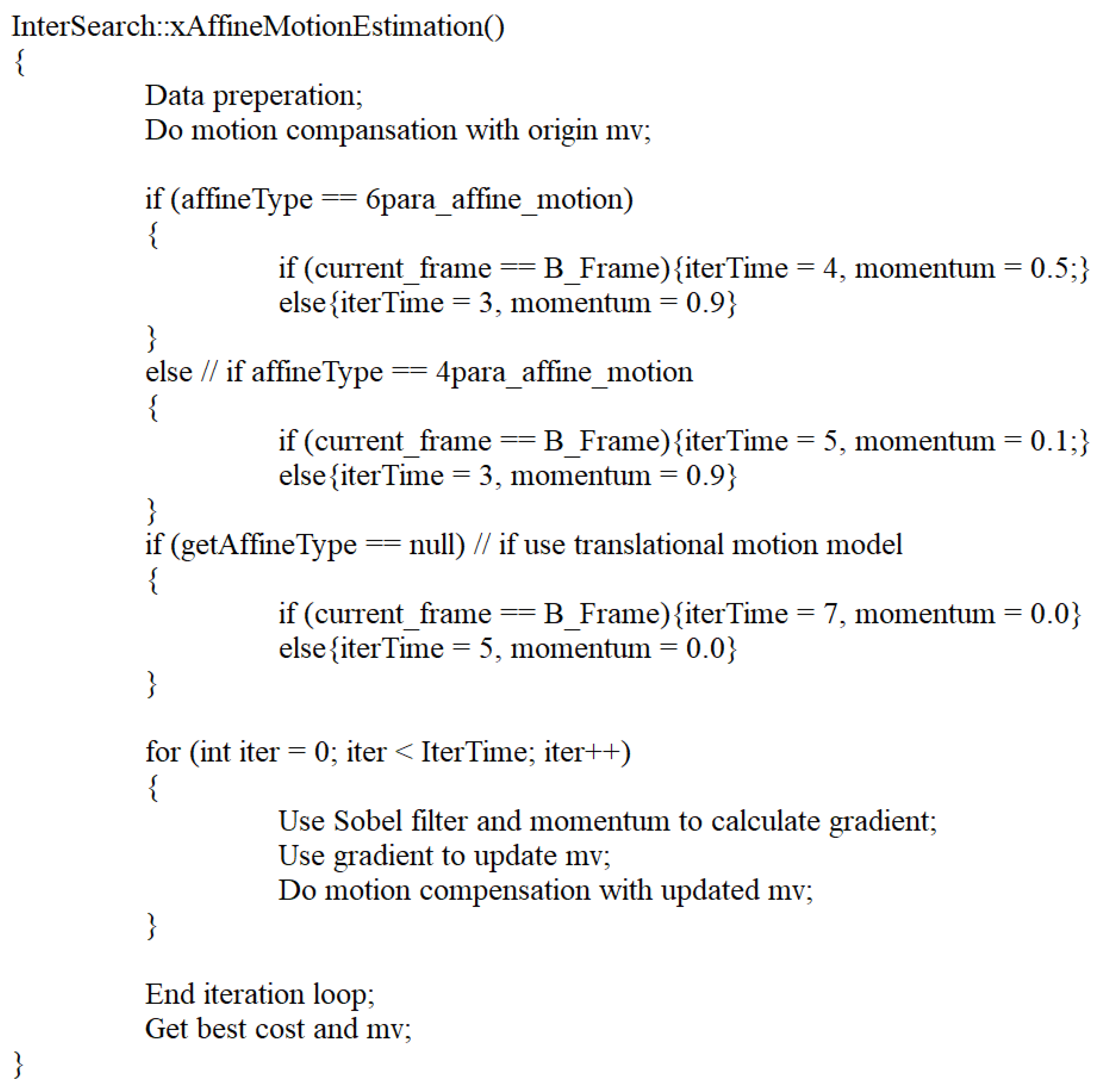
Additionally, to avoid shocks in the search iteration or convergence on the extremum of the gradient that is too slow, we add momentum, a constant, to solve this problem. When the gradient in this iteration has the same direction as the gradient in the last iteration in the x or y direction, the momentum plays an accelerating role in this search. Otherwise, the momentum can slow down the gradient change:

$$\{\begin{array}{c}{\mathrm{grad}}_{\mathrm{x}}^{\mathrm{i}}{=\mathrm{grad}}_{\mathrm{x}}^{\mathrm{i}}+\mathrm{momentum}·{\mathrm{grad}}_{\mathrm{x}}^{\mathrm{i}-1}\\ {\mathrm{grad}}_{\mathrm{y}}^{\mathrm{i}}{=\mathrm{grad}}_{\mathrm{y}}^{\mathrm{i}}+\mathrm{momentum}·{\mathrm{grad}}_{\mathrm{y}}^{\mathrm{i}-1}\end{array}$$

(24)

The pseudocode of momentum in AMC is described by Figure 7:

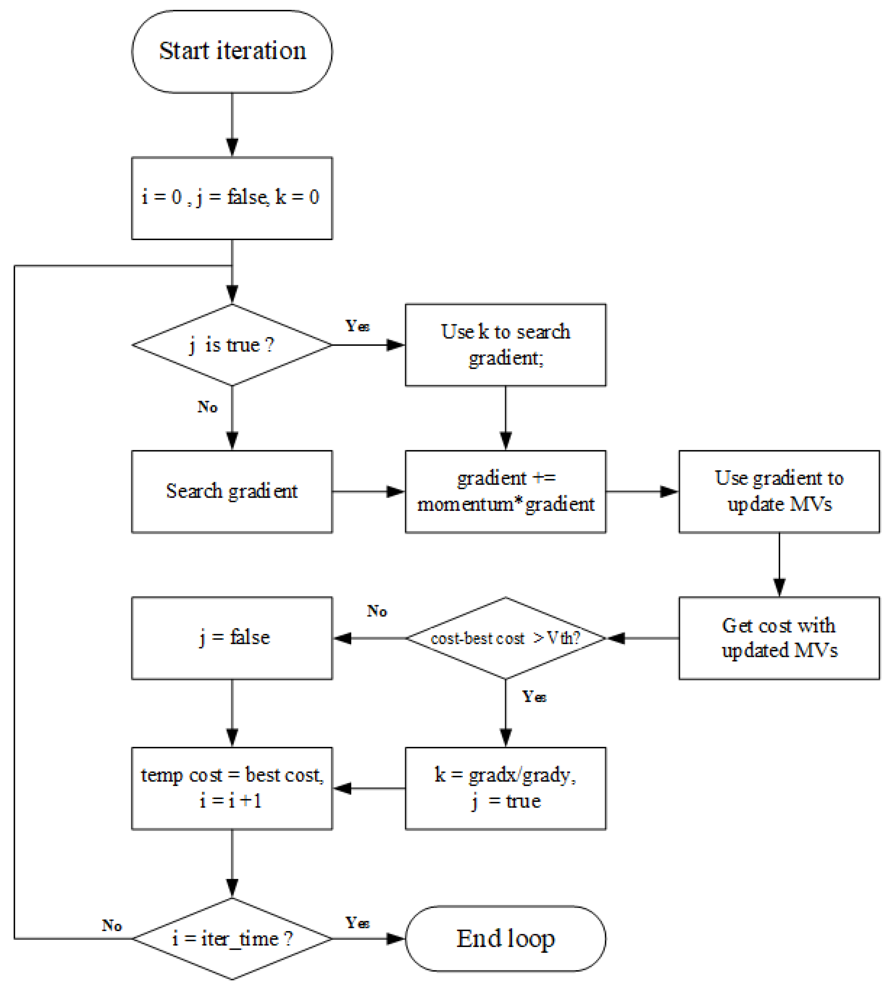
Combining these proposed methods, Figure 8 shows the flow chart for the modified AMC process:

The specific steps are:

• Initialize iteration time i, sign j and coefficient k at the beginning of iteration.
• Check j and enable the fast gradient search when the sign is true, otherwise enable the conventional gradient search. The fast gradient search uses the coefficient k and the gradient in the horizontal or vertical direction to predict the gradient in another direction. In this case, only one array of gradient is called upon to solve the derivate.
• Add momentum to update the gradient and then use gradient to update the MVs and obtain cost with the updated MVs.
• Use the cost change of distortion as the sign for enabling fast gradient search. Set j to be true and update k with the gradient when:

$${\mathrm{temp}\mathrm{cost}-\mathrm{best}\mathrm{cost}>\mathrm{V}}_{\mathrm{th}}$$

(25)

Otherwise set j to false.

• Update i and the temp cost with the best cost in the current iteration. The encoder ends the iteration loops when i reaches the maximum of iteration time.

3.2. AAMVP for 6-Parameters

In this subsection, we propose a modified AAMVP for 6-parameters according to the symmetry of AAMVP for 4-parameters in VVC. HEVC provides two typical methods for determining the translational MV: AMVP mode combined with fast ME algorithm; and merge mode.

AAMVP in VVC builds a sorted MVP candidate list for the 4-parameter affine motion model by using ${\mathrm{MV}}_2$, belonging to the tuple ${\mathrm{S}}_2$ for the combination’s priority determination, which is signaled explicitly to the lists and thus cannot be used for priority determination. We propose a new judgment rule for AAMVP for the 6-parameter affine motion model.

Because the VVC encoder predicts the affine model adaptively, increasing the probability that the current MV combination forms a 4-parameter affine motion model with a smaller $\mathrm{DMV}$ in Formula (13), when the encoder chooses the 6-parameter affine motion model for prediction, the current MV combination should be less likely to form the 4-parameter affine motion model.

In most sequences, the encoder uses the 6-parameter affine motion model instead of the 4-parameter affine motion model to characterize complex motions like shearing. Figure 9 shows an example of the 6-parameter affine motion model with shearing:

where ${\mathrm{MV}}_0$,${\mathrm{MV}}_1$ and ${\mathrm{MV}}_2$ are MVP candidates that belong to the tuples ${\mathrm{S}}_0$,${\mathrm{S}}_1$ and ${\mathrm{S}}_2$. This shows that $\frac{{\mathrm{MV}}_1^{\mathrm{h}}{-\mathrm{MV}}_0^{\mathrm{h}}}{\mathrm{w}-1}$ and $\frac{{\mathrm{MV}}_0^{\mathrm{v}}{-\mathrm{MV}}_1^{\mathrm{v}}}{\mathrm{w}-1}$ reflect the affine transformation of the unit width or unit height of the current block’s width in the horizontal and vertical directions, while $\frac{{\mathrm{MV}}_2^{\mathrm{h}}{-\mathrm{MV}}_0^{\mathrm{h}}}{\mathrm{h}-1}$ and $\frac{{\mathrm{MV}}_2^{\mathrm{v}}{-\mathrm{MV}}_0^{\mathrm{v}}}{\mathrm{h}-1}$ reflect the average affine transformation degree of the current block’s length in the horizontal and vertical directions.

By using the similarity of triangles, we can conclude that, with respect to blocks with small degrees of deformation, the change of the width in the horizontal direction should be close to that of the height in the vertical direction, while the change of the height in the horizontal direction should be close to that of the width in the vertical direction. Then we have:

$${\mathrm{DMV}}_6=\left|\left(\mathrm{h}-1\right)·\left({\mathrm{MV}}_1^{\mathrm{h}}{-\mathrm{MV}}_0^{\mathrm{h}}\right)-\left(\mathrm{w}-1\right)·\left({\mathrm{MV}}_2^{\mathrm{v}}{-\mathrm{MV}}_0^{\mathrm{v}}\right)\right|+\left|\left(\mathrm{h}-1\right)·\left({\mathrm{MV}}_2^{\mathrm{h}}{-\mathrm{MV}}_0^{\mathrm{h}}\right)-\left(\mathrm{w}-1\right)·\left({\mathrm{MV}}_0^{\mathrm{v}}{-\mathrm{MV}}_1^{\mathrm{v}}\right)\right|$$

(26)

With a higher value of ${\mathrm{DMV}}_6$, it will be more likely that ${\mathrm{MV}}_0$,${\mathrm{MV}}_1$ and ${\mathrm{MV}}_2$ form a real 6-parameter affine motion model rather than a 4-parameter affine motion model. We transmit the two $\left({\mathrm{MV}}_{0,}{\mathrm{MV}}_1{,\mathrm{MV}}_2\right)$ with the biggest and second biggest $\mathrm{DM}{\mathrm{V}}_6$ to the AAMVP candidate list after the traversal ends.

4. Experimental Results

4.1. Simulation Setup

In this part, we evaluate the performance of the proposed algorithms based on the VVC test model (VTM) and the symmetrical general VVC test model with AMC disabled/enabled. This experiment is based on the VTM-7.0 anchor [16], which was released in December 2019 and was the most recent version released during the experiment. The VTM-7.0 anchor defines different configuration files for different applications, including all I-frame (AI), random access (RA), low delay P (LP) and low delay B (LB). The test video sequence adopts the video sequence from class A to class F under general test conditions [17], the resolution of which ranges from 416 × 240 to 2560 × 1600. The specific simulation environment is shown in

Table 1. Simulation environment.

Processor	Inter(R) Core (TM) i5-8400 CPU @ 2.80GHz
Core number	6
memory	16.0GB
cache	9MB
Operating system	Windows 10 × 64
IDE	Microsoft Visual Studio 16 2019

.

The Bjøntegaard Delta Bitrate (BD-BR) [18] is employed in our experiments to provide a fair R-D performance comparison. The quantization parameters (QPs) tested are 22, 27, 32, and 37, and the change of encoding time computed for each of the four tested QPs for each sequence using the following formula to calculate the mean value:

$$\Delta \mathrm{T}=\frac{1}{4}{\displaystyle \sum }_{\mathrm{i}=1}^4\frac{{\mathrm{T}}_{\mathrm{tested}}^{\mathrm{i}}{-\mathrm{T}}_{\mathrm{anchor}}^{\mathrm{i}}}{{\mathrm{T}}_{\mathrm{anchor}}^{\mathrm{i}}}\times 100\%$$

(27)

where i denotes each different quantization parameter: 22, 27, 32 and 37, the ${\mathrm{T}}_{\mathrm{tested}}^{\mathrm{i}}$ denotes the encoding time for the tested encoder and ${\mathrm{T}}_{\mathrm{anchor}}^{\mathrm{i}}$ denotes the encoding time for the anchor encoder. The encoding time increases when $\Delta \mathrm{T}$ is positive and decreases when $\Delta \mathrm{T}$ is negative.

4.2. Performance and Analysis

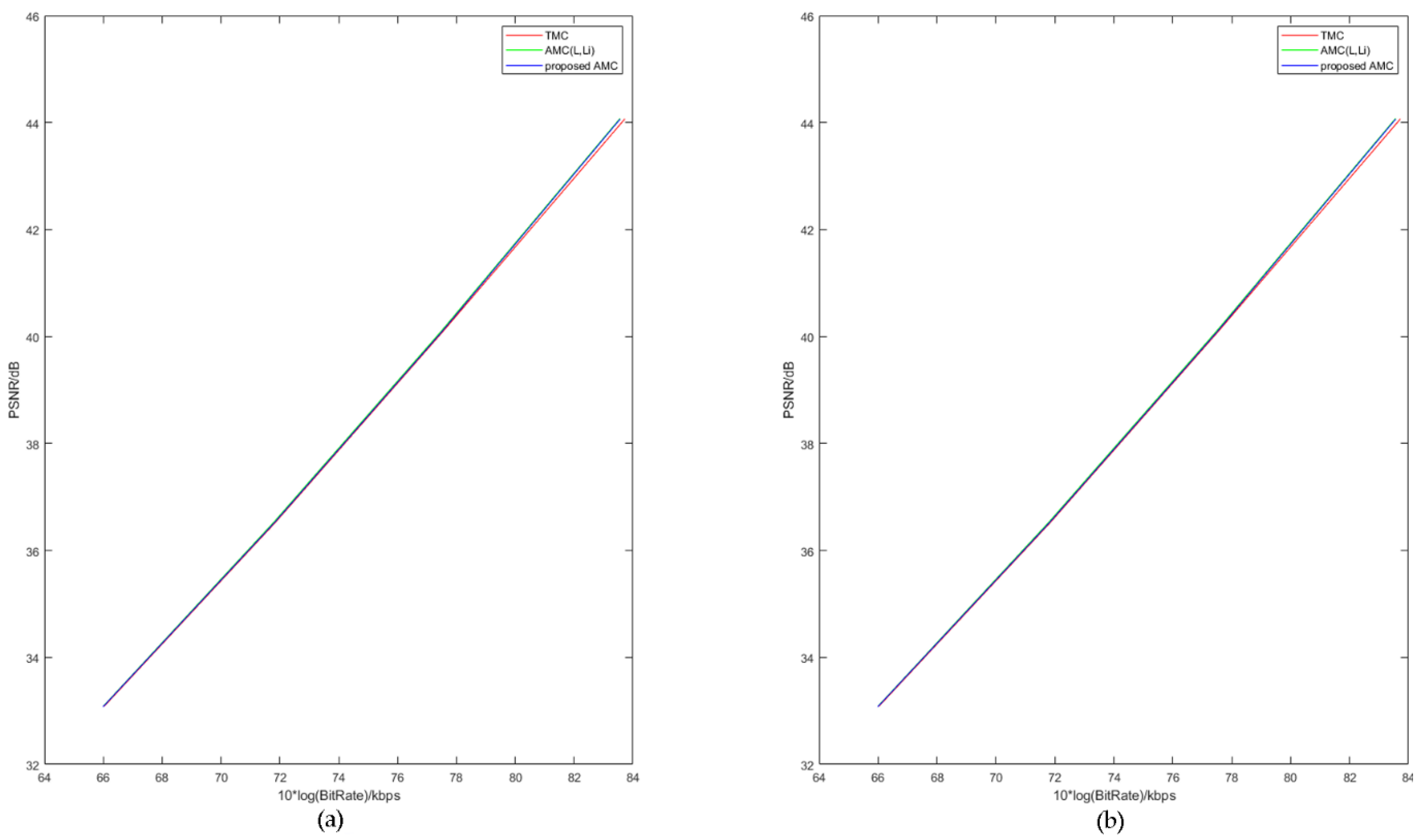
First, we use the VTM-7.0 with TMC as the anchor encoder and test the performance of the AMC proposed by L. Li [10] and our proposed AMC. The AMC proposed in [10] has been accepted as the VVC standard, and has been used in VTM-7.0. The x-axis and y-axis of the rate–distortion curves are bitrate and distortion. Usually, less distortion requires a higher bitrate. The rate–distortion curves of some video sequences are shown in Figure 10.

Where the x-axis represents the bitrate of tested video sequences, and the y-axis represents the average peak signal-to-noise ratio (PSNR). Under the same bitrate, higher PSNR means less distortion and better reconstructed video quality. Figure 10 shows similar rate–distortion performances between the AMC proposed by L. Li [10], which was based on the anchor encoder of HM-16.7 in HEVC, and our proposed AMC. The RD curves of our proposed AMC are a bit lower.

To separately observe the effect of proposed algorithm in AMC, we first tested the performance of the AMC encoder using only momentum to calculate gradients.

Table 2. Performances of 4-Parameter AMC and AMC with momentum.

Class	Sequences	Encoded Frames	AMC (L. Li et al.)		AMC with Momentum
			BDBR (%)	ΔT (%)	BDBR (%)	ΔT (%)
A	Traffic	60	−15.83	21.31%	−15.85	21.36%
	PeopleOnStreet	60	−16.23	22.09%	−16.24	22.11%
B	ParkScene	120	−17.04	17.83%	−17.08	17.89%
	BQTerrace	120	−16.2	19.57%	−16.23	19.74%
	BasketballDrive	100	−23.32	18.61%	−23.35	18.70%
	Cactus	100	−31.13	19.81%	−31.16	19.84%
	kimono	120	−18.89	20.08%	−18.9	20.09%
C	BQMall	240	−15.71	21.55%	−15.71	21.59%
	PartyScene	200	−20.01	22.63%	−20.04	22.65%
	RaceHorses	120	−19.73	25.65%	−19.74	25.66%
	BasketballDrill	200	−21.17	20.17%	−21.2	20.18%
D	BQSquare	240	−22.99	18.78%	−23.02	18.79%
	BlowingBubbles	200	−15.21	18.18%	−15.23	18.21%
	BasketballPass	200	−21.8	21.61%	−21.82	21.64%
E	Johnny	120	−20.75	39.62%	−20.75	39.63%
	KiristenAndSara	120	−18.74	23.50%	−18.77	23.54%
	FourPeople	120	−20.24	24.01%	−20.25	24.02%
F	ChinaSpeed	150	−70.52	14.28%	−70.54	14.30%
	SlideShow	200	−41.31	19.66%	−41.35	19.67%
	SlideEditing	150	−19.13	14.55%	−19.15	14.58%
	BasketballDrillText	200	−19.98	21.08%	−20.01	21.11%
average			−23.14	21.17	−23.16	21.20%

shows that the BD-BR increases by about 0.02%, while the encoder time increases by about 0.03%, on average. For each iteration in AMC, the value of momentum is a constant, and MVs of the last iteration are stored in the array, thus resulting in a linear increase in time complexity. This part of the algorithm added little complexity to the increase in BD-BR.

Then, we compared the performance of the AMC and AMC with the proposed AAMVP of the 6-parameter affine motion model. The results are shown in

Table 3. Performances of AMC (L. Li et al.) and AMC with AAMVP.

Class	Sequences	Encoded Frames	AMC (L. Li et al.)		AMC with AAMVP
			BDBR (%)	ΔT (%)	BDBR (%)	ΔT (%)
A	Traffic	60	−15.83	21.31%	−15.83	21.09%
	PeopleOnStreet	60	−16.23	22.09%	−16.23	21.78%
B	ParkScene	120	−17.04	17.83%	−17.04	17.42%
	BQTerrace	120	−16.2	19.57%	−16.2	19.14%
	BasketballDrive	100	−23.32	18.61%	−23.32	17.02%
	Cactus	100	−31.13	19.81%	−31.13	19.17%
	kimono	120	−18.89	20.08%	−18.89	19.44%
C	BQMall	240	−15.71	21.55%	−15.71	21.04%
	PartyScene	200	−20.01	22.63%	−20.01	22.20%
	RaceHorses	120	−19.73	25.65%	−19.73	24.76%
	BasketballDrill	200	−21.17	20.17%	−21.17	19.34%
D	BQSquare	240	−22.99	18.78%	−22.99	18.49%
	BlowingBubbles	200	−15.21	18.18%	−15.21	17.74%
	BasketballPass	200	−21.8	21.61%	−21.8	21.30%
E	Johnny	120	−20.75	39.62%	−20.75	38.05%
	KiristenAndSara	120	−18.74	23.50%	−18.74	23.11%
	FourPeople	120	−20.24	24.01%	−20.24	23.25%
F	ChinaSpeed	150	−70.52	14.28%	−70.52	13.14%
	SlideShow	200	−41.31	19.66%	−41.31	19.28%
	SlideEditing	150	−19.13	14.55%	−19.13	14.12%
	BasketballDrillText	200	−19.98	21.08%	−19.98	20.11%
average			−23.14	21.17	−23.14	20.52%

.

Table 3 shows that the proposed AAMVP for the 6-parameter affine motion model changes the priority of the AMVP list’s candidates, and this will not affect the BD-BR, but can reduce the encoder time by 0.65% on average. On those sequences with more complex affine motion, the effect of the proposed AAMVP is better.

To observe the performances more specifically in different classes of videos, we compared the performance of the AMC and our proposed AMC combining momentum, fast gradient search and AAMVP by using BD-BR. Their performances are shown in

Table 4. Performances of AMC (L. Li et al.) and Proposed AMC.

Class	Sequences	Encoded Frames	AMC (L. Li et al.)		Proposed AMC
			BDBR (%)	ΔT (%)	BDBR (%)	ΔT (%)
A	Traffic	60	−15.83	21.31%	−15.71	14.29%
	PeopleOnStreet	60	−16.23	22.09%	−16.09	14.79%
B	ParkScene	120	−17.04	17.83%	−16.95	11.43%
	BQTerrace	120	−16.20	19.57%	−16.15	12.57%
	BasketballDrive	100	−23.32	18.61%	−23.14	14.17%
	Cactus	100	−31.13	19.81%	−30.89	13.69%
	kimono	120	−18.89	20.08%	−18.74	13.60%
C	BQMall	240	−15.71	21.55%	−15.57	15.68%
	PartyScene	200	−20.01	22.63%	−19.86	15.94%
	RaceHorses	120	−19.73	25.65%	−19.58	16.87%
	BasketballDrill	200	−21.17	20.17%	−20.88	15.95%
D	BQSquare	240	−22.99	18.78%	−22.63	13.24%
	BlowingBubbles	200	−15.21	18.18%	−15.19	14.01%
	BasketballPass	200	−21.80	21.61%	−21.27	14.82%
E	Johnny	120	−20.75	39.62%	−20.59	21.42%
	KiristenAndSara	120	−18.74	23.50%	−18.61	17.07%
	FourPeople	120	−20.24	24.01%	−20.05	14.88%
F	ChinaSpeed	150	−70.52	14.28%	−69.71	11.59%
	SlideShow	200	−41.31	19.66%	−40.89	13.17%
	SlideEditing	150	−19.13	14.55%	−19.09	10.70%
	BasketballDrillText	200	−19.98	21.08%	−19.89	14.98%
average			−23.14	21.17	−22.93	14.52

.

Table 4 shows that the AMC exhibited improved performance when compared with the TMC. Some sequences present outstanding performance under the AMC framework, showing both bitrate saving and increase in PSNR in all QPs. With respect to these sequences, “Cactus” contains abundant rotation motions, while “Slideshow” shows a PowerPoint slide with many artificial shearing motions. It should be noted that the BDBR of “China Speed” can be reduced by up to about 70%.

Additionally, under the AMC framework, the BDBR decreases by 23.14% on average, and the average encoding time increases by 21.17%. Table 2 also shows that the proposed algorithm provides 22.93% BDBR saving and 14.52% time increase compared with the TMC. When compared to the AMC proposed by L. Li [10], the coding time is reduced by 6.65% on average, with a cost of 0.21% BDBR penalty, which means the proposed algorithm reduces the coding time of the AMC by about 30%. Noted that for sequences with poor performance, such as “China Speed”, the BDBR penalty is 0.81%. This might be because the objects exhibit fast affine motion, and the gradients are not smooth, thus degrading the performance of the fast gradient search.

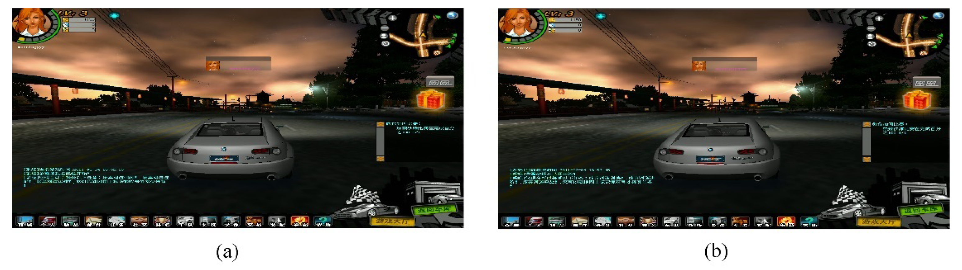
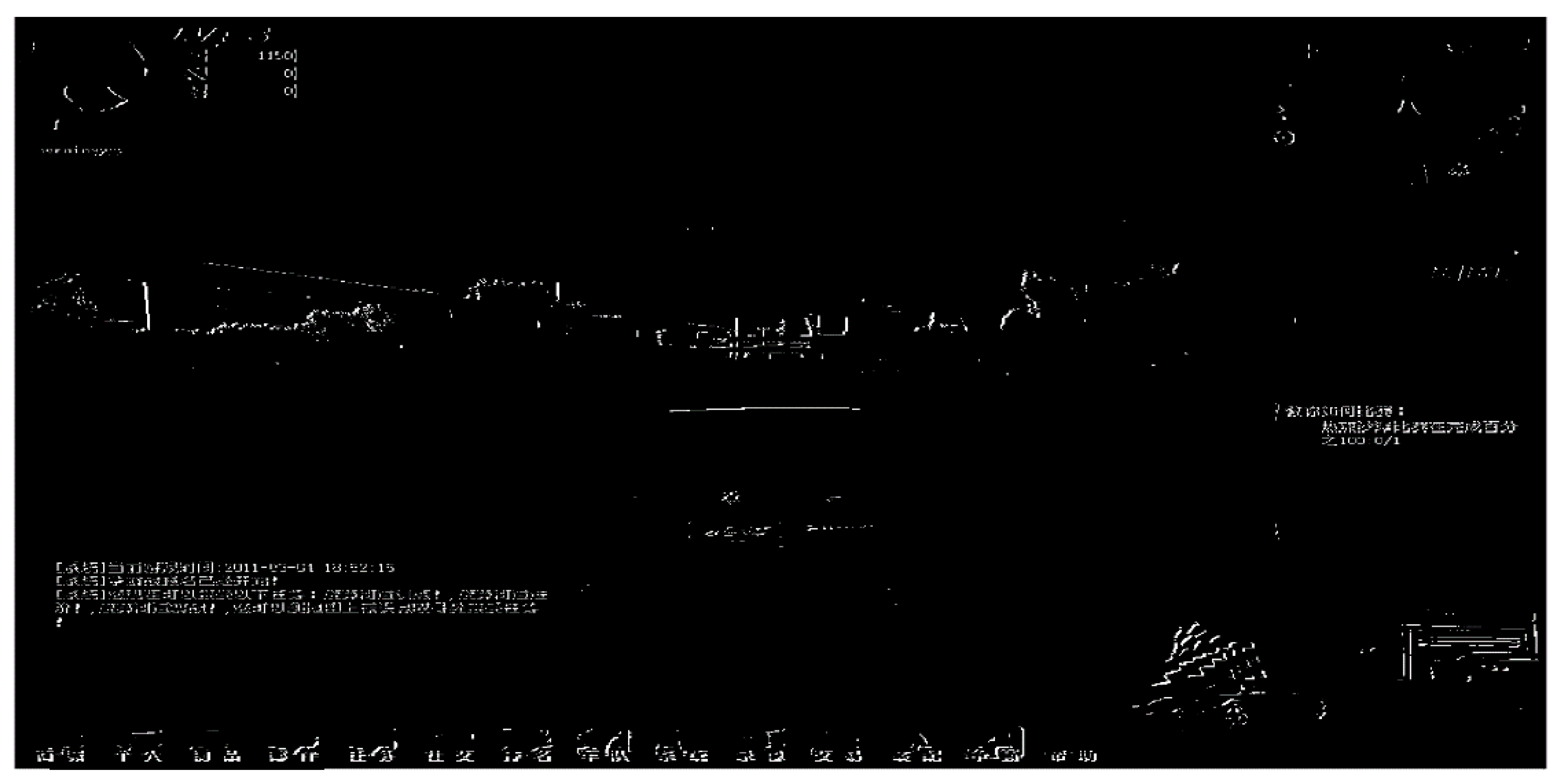
Still, the algorithm will not reduce the subjective quality of the sequence. Figure 11 shows a comparison of the origin and reconstructed image with QP22, random access. By subtracting these two pictures, Figure 12 shows the distortion of the reconstructed image. The example picture size is 1024 × 768 and the MSE is 912.

5. Conclusions

The AMC frame, which has previously been adopted in VVC coding, saves approximately 15%-25% BD-rate compared to HEVC, but increases the encoding time. In this paper, we firstly introduce the 4-parameter affine motion compensation and multiple model affine motion compensation in VVC and analyze their performances. Then, a VVC encoder with an edge detection based AME was introduced and tested. A new edge detection operator and a distortion-based fast gradient search were used in this proposed VVC encoder. Additionally, we adjust the AAMVP criterion for the 6-parameter affine motion model. Ultimately, the proposed VVC encoder reduced the coding time by 6.65% with a cost of a 0.21% BDBR penalty compared to the anchor encoder. Considering that the anchor AMC frame increases the coding time by 21.17% on average, the proposed algorithms can save 30% of encoding time of AMC. The BDBR inevitably increases, but this is tolerable, and the subjective video quality is not affected.

References

- Wiegand, T.; Sullivan, G.J.; Bjøntegaard, G.; Luthra, A. Overview of the H.264/AVC video coding standard. IEEE Trans. Circuits Syst. Video Technol. 2003, 13, 560–576. [Google Scholar] [CrossRef] [Green Version]
- Sullivan, G.J.; Ohm, J.-R.; Wiegand, T.; Han, W.-J. Overview of the High Efficiency Video Coding (HEVC) Standard. Circuits Syst. Video Technol. 2012, 22, 1649–1668. [Google Scholar] [CrossRef]
- Ohm, J.-R.; Sullivan, G.J.; Schwarz, H.; Tan, T.K.; Wiegand, T. Comparison of the Coding Efficiency of Video Coding Standards—Including High Efficiency Video Coding (HEVC). IEEE Trans. Circuits Syst. Video Technol. 2012, 22, 1669–1684. [Google Scholar] [CrossRef]
- Bross, B. Versatile Video Coding (Draft 1); JVET-J1001; Joint Video Exploration Team (JVET): San Diego, CA, USA, 2018. [Google Scholar]
- Li, L.; Li, H.; Lv, Z.; Yang, H. An affine motion compensation framework for High Efficiency Video Coding. In Proceedings of the 2015 IEEE International Symposium on Circuits and Systems (ISCAS), Lisbon, Portugal, 24–27 May 2015; pp. 525–528. [Google Scholar]
- Zhang, K.; Chen, Y.; Zhang, L.; Chien, W.; Karczewicz, M. An Improved Framework of Affine Motion Compensation in Video Coding. IEEE Trans. Image Process. 2019, 28, 1456–1469. [Google Scholar] [CrossRef] [PubMed]
- Chen, Y.-W.; Chien, W.J.; Chuang, H.C. Description of SDR, HDR and 360° Video Coding Technology Proposal by Qualcomm and Technicolor—Low and High Complexity Versions; Document JVET–J0021; Joint Video Exploration Team (JVET): San Diego, CA, USA, 2018. [Google Scholar]
- Seferidis, V.E.; Ghanbari, M. General approach to block-matching motion estimation. Opt. Eng. 1993, 32, 1464–1474. [Google Scholar] [CrossRef] [Green Version]
- Huang, H.; Woods, J.W.; Zhao, Y.; Bai, H. Control-point representation and differential coding affine-motion compensation. IEEE Trans. Circuits Syst. Video Technol. 2013, 23, 1651–1660. [Google Scholar] [CrossRef]
- Li, L.; Li, H.; Liu, D.; Li, Z.; Yang, H.; Lin, S.; Chen, H.; Wu, F. An Efficient Four-Parameter Affine Motion Model for Video Coding. IEEE Trans. Circuits Syst. Video Technol. 2018, 28, 1934–1948. [Google Scholar] [CrossRef] [Green Version]
- Li, B.; Xu, J.; Li, H. Parsing robustness in high efficiency video coding—Analysis and improvement. In Proceedings of the IEEE Visual Communications and Image Processing (VCIP), Tainan, Taiwan, 6–9 November 2011; pp. 1–4. [Google Scholar]
- Zhu, W.; Ding, W.; Xu, J.; Shi, Y.; Yin, B. Hash-Based Block Matching for Screen Content Coding. IEEE Trans Multimed. 2015, 17, 935–944. [Google Scholar] [CrossRef]
- Tsai, T.; Su, S.; Lee, T. Fast mode decision method based on edge feature for HEVC inter-prediction. IET Image Process. 2018, 12, 644–651. [Google Scholar] [CrossRef]
- Shi, W.; Jiang, X.; Song, T.; Shimamoto, T. Edge information based fast selection algorithm for intra prediction of HEVC. In Proceedings of the 2014 IEEE Asia Pacific Conference on Circuits and Systems (APCCAS), Ishigaki, Okinawa, Japan, 17–20 November 2014; pp. 17–20. [Google Scholar]
- Wieckowski, A.; Ma, J.; Schwarz, H.; Marpe, D.; Wiegand, T. Fast Partitioning Decision Strategies for The Upcoming Versatile Video Coding (VVC) Standard. In Proceedings of the 2019 IEEE International Conference on Image Processing (ICIP), Taipei, Taiwan, 22–25 September 2019; pp. 4130–4134. [Google Scholar]
- VTM-7.0. Available online: https://vcgit.hhi.fraunhofer.de/jvet/VVCSoftware_VTM/-/tree/VTM-7.0. (accessed on 15 December 2019).
- Suehring, K.; Li, X. JVET Common Test. Conditions and Software Reference Configurations; Document JVET-G1010; Joint Video Experts Team: San Diego, CA, USA, 2017. [Google Scholar]
- Bjøntegaard, G. Calculation of Average PSNR Differences between RD Curves; Document ITU-T SG.16 Q.6, VCEG-M33; Video Coding Experts Group (VCEG): Austin, TX, USA., 2001. [Google Scholar]
Figure 1.
Three typical motions: (a) rotation, (b) translation, (c) zooming.
Figure 2.
The 4-parameter affine motion model with two Control-points.
Figure 3.
The 6-parameter affine motion model with three Control-points.
Figure 4.
The AMVP candidate list.
Figure 5.
An example of AAMVP.
Figure 6.
Choices of the AMM candidates.
Figure 7.
The pseudocode of momentum in AMC.
Figure 8.
The flow chart for the proposed algorithm.
Figure 9.
An example of the 6-parameter affine motion model.
Figure 10.
The rate–distortion curves with three kinds of motion compensation. (a) Performances of the sequence “China Speed”. (b) Performances of the sequence “Park Scene”.
Figure 11.
The comparation of the reconstructed image quality, ChinaSpeed, RA, QP22, POC1: (a) the original image, (b) the reconstructed image with the proposed algorithm.
Figure 12.
The distortion of the reconstructed image and the original image quality.