Local and Global Welfare When Regulating Organic Products: Should Local Regulation Target Production or Consumption?

Abstract

Based on a welfare approach using a partial equilibrium model coming from microeconomics, this paper analyzes whether a local regulation aimed at reducing risks due to pesticides should be imposed at the production level or the consumption level. This paper characterizes the economic impact of these possible regulations from a theoretical point of view. Local and nonlocal producers compete only in the local market regarding selling conventional and organic products. Local producers incur variable costs related to reducing the risk of damage resulting from their new organic production methods. A local policymaker maximizing local welfare chooses either a regulation that is imposed on its local producers via production requirements or on all local and nonlocal producers via retail requirements that directly affect consumption. We show that local regulation is selected for relatively large values of damage. In this case, the organic regulation is influenced by whether the damage is incurred by residents and the environment close to the production site or by consumers. If the damage is incurred by residents and the environment close to the production site, only regulations targeting the local producers are selected, which improves the profits for nonlocal producers. Concerning damage incurred by consumers after their consumption, each type of regulation is selected depending on the cost of the safe technology, but the regulation targeting the consumption level harms nonlocal producers.

1. Introduction

Modern conventional agriculture brings about high labor productivity and output. However, due to the massive use of agricultural chemicals such as synthetic fertilizers and pesticides, both the environment and foods are polluted to varying degrees. In particular, the ecosystems are damaged, and the land’s production capacity continues to decline. Though people have come to know that organic agriculture has its inherent deficiencies, they prefer to believe that organic agriculture switches to a direction favorable for economic development, dietary improvement, and sustainable farming. In this context, organic agriculture has gained momentum over the last 30 years, and policymakers have tried to develop regulations for providing sufficient incentives to farmers to adopt organic farming. As regulators cannot impose organic practices on all farmers, some regulations take a local form. Indeed, new solutions could consist of developing local organic regulations imposing organic practices at a regional level. By considering local comparative advantages, local regulations are less drastic than broad and national regulations.

In India, the state of Sikkim offers an interesting example of ambitious organic regulation. Since 2003, chemical pesticides have been phased out in Sikkim [1]. After several rounds of regulatory efforts, Sikkim completely banned chemical pesticides and synthetic fertilizers in 2016, forcing their farmers to use organic processes and alternative agronomic practices. Organic agriculture switches to a direction favorable for the environmental development of Sikkim, with improvements in environmental indicators [2]. This new system has been able to provide jobs and support social interactions between producers and consumers. Moreover, the Sikkim regulation also focuses on consumption and market expansion, health, education, rural development, and sustainable tourism. As such, Sikkim is an excellent model for other Indian states and countries worldwide who want to upscale their agroecology [2]. On the other hand, this generalized organic farming puts the agricultural development of Sikkim at risk. More particularly, yields have fallen for many crops since all producers switched to organic farming in 2016 [3]. Moreover, because of low purchasing power and a limited understanding of the benefits of organic production, local consumers are reluctant to pay higher prices for these organic products and prefer buying conventional products from border states [4]. As a result, some local producers have reported losses related to lower yields and difficulties selling products. The goal of organic farming in developed countries is currently about meeting the needs of those who can afford the luxury of buying the highest quality food. If the needs of this luxury interfere with the need to feed the entire and fragile population, then you have the potential for conflict. The cost–benefit of this local regulation is still complex, and there are difficult trade-offs to consider for the local regulator.

To understand these trade-offs coming from local organic regulation, one solution consists of examining the results of previous articles. There are many contributions regarding the role of labeling and its positive impact on consumers’ willingness to pay around the world [5]. In the following paragraphs, we restrict our attention to papers examining the impact of organic regulation on producers.

More particularly, the numerous contributions focusing on the risks of organic regulation for producers can be divided into three categories that are presented as follows. First, regulation might bring many risks to producers. Risks are reflected in many spheres, such as production risk, which includes plant contamination of organic production from genetically modified organisms [6]; a potential health risk from heavy metalloids caused by cropping systems [7]; environmental risk, which includes ecoregion-specific ecotoxicological evaluations of pesticides [8]; management risk, which includes the quality of the ingredients and the integration of food safety systems for industrial growth [9]; financial risk, which includes little knowledge of crop insurance by farmers [6]; market risk, which includes maximum residue limits of pesticide regulation set by the importing countries and exporting country [10]; and institutional risk, which includes, without objectively defining and consequently assessing the standards, a fair amount of disagreement about what constitutes organic food [11].

Second, the characteristics of organic regulations might also make the production task more complex for farmers. The inherent characteristics of current regulations are manifested in many aspects, such as the lack of regulation in working near animal housing facilities, which harm farm staff through odorous nuisance [12]; current unreasonable regulations for soils, which might not be effective in protecting human health or harmonizing downstream food [13]; the disunity of regulations in different countries, which might bring organic food quality risks through using different plant protection products [14]; and changing regulations, which might bring potential risks due to farmers with a limited capacity of information development and utilization [15,16].

Third, the efficiency of regulatory options might be affected by producer heterogeneity. The producer’s heterogeneity is embodied in many ways, such as producers planting different crop varieties, which may include spinach accumulating almost two times more perchlorate than chard for all treatments [17]; producers in different economic areas that may not have sufficient access to certification or markets for crop farmers in poor areas [13]; producers in different environmental areas that can adversely impact the safety of honey under the mining field [18]; producers in different operation modes in which contract farming can reduce pollution more than noncontract farming [19]; and producers entering the organic sector with different time spans in which early adopters pay more attention to the environmental and healthy aspects of organic agriculture, whereas late adopters consider the economic benefits of organic farming more [20].

The existing research has performed a comprehensive analysis of organic regulation on the producer. However, there is still a lack of research on the economic welfare risk of organic regulation. Risk analysis is beneficial to a holistic planning process aimed at making better decisions and emphasizing the connections between the parts [21], and welfare analysis is more conducive to understanding the effect of these regulations [22,23]. Lacking clarity about the interest changes and potential risk patterns at home and abroad brought by local regulations, the central government cannot guide the development of regulations, which might hinder the healthy development of organic agriculture. Therefore, local regulations targeting the production level or the consumption level for reducing producer risks are becoming a topic worthy of study.

Aimed at showing the complexity of market adjustments under local or global regulations, the theoretical model presented in the following sections vastly oversimplifies the notions of local and global entities. The term “local” means a relatively large area instead of a tiny place with a few farmers, and it refers to any specific sales market where there is a demand for organic agricultural production and where organic regulations can be effectively implemented to ensure the interests of consumers. A local entity can impose a regulation to both local and/or foreign producers selling products on its territory, without more details about the frontiers and the controls at the borders. Meanwhile, a local entity can encompass various forms of regions or states included in a vast political union, which may correspond to the Sikkim situation in India (see above), or to a Member State in the European Union (EU). Taking the EU as an example in terms of policymaking, since the new Common Agricultural Policy (CAP) recently “re-nationalized” some policies, some environmental policies now depend on decisions at the national or regional level. In such a context of Member States’ autonomy, one possible pathway for the future would consist of having an ambitious national agenda like a high level of organic productions, representing 50% or even 100% of the production (or consumption) as the extreme configuration studied in this paper. A national decision, such a drastic regulation could also be taken by the European Parliament, epitomizing a global regulation at the EU level. Beyond this example, the model abstracts from legal considerations regarding local or global regulations for focusing on an extremely simple configuration allowing economic analysis.

The following study uses a simplified welfare analysis method for evaluating the impact of local policies. A local policymaker maximizing local welfare chooses a regulation that is imposed either on its local producers via production requirements or on all producers via consumption requirements. In our simple model, a local policymaker takes into account the local welfare, defined as the sum of all economic gains and losses for agents living in a given area. We compare this local regulatory choice to a global regulatory choice maximizing the global welfare inclusive of all agents.

We show that the regulation is selected for relatively large values of damage. In this case, the regulation is influenced by the nature of the damage, either damage incurred by residents and the environment close to the production site or damage incurred by consumers after consumption. With damage incurred by residents and the environment close to the production site, only the regulation targeting the local producers is selected, which improves the profits for nonlocal producers. With damage incurred by consumers after consumption, each type of regulation is selected depending on the cost of the safe technology, but the regulation targeting the consumption level harms nonlocal producers.

Our paper differs from previous contributions by detailing the consequences of local organic regulations. Our approach contributes to the literature focusing on the significant and large development of organic farming with questions regarding its feasibility. For instance, Muller et al. [24] underscore that a 100% conversion to organic agriculture effectively reduces pesticide use but needs more land than conventional agriculture. This increase in land use comes from the necessity to outweigh the reduction of yields coming from organic conversion [25]. Our paper differs because our “regional conversion” is less drastic than a 100% conversion, and we focus on the economic approach by measuring both price and quantity distortions.

Our paper focuses on local regulation versus global regulation, which is very close to the questions related to non-tariff measures for evaluating regulation [22]. More particularly, Fisher et al. [26] show that in the presence of a production/consumption externality, the standard chosen by the social planner is always protectionist—namely, it harms the foreign producers (or the nonlocal producer), with the marginal costs for reducing risks being internalized into market prices [27,28,29]. However, the present paper underlines the opposite result. Our paper contributes by showing that nonlocal producers may benefit from the local regulation of local organic production because this process reduces competition in the conventional product segment. We also show that the selected regulation is influenced by the damage incurred at either the production level or the consumption level, which is an issue overlooked by previous articles.

Ultimately, our paper contributes to the theoretical research on regulation. It differs from contributions in which expected damage, proportional to the output, incurred by residents close to the production or by consumers makes no major difference. Indeed, as all agents belong to the same economy in classical studies [30], there is no difference in whether the damage is incurred at the production level or the consumption level.

This paper is structured as follows. An analysis model is introduced in Section 2. Section 3 presents market mechanisms and regulations. Section 4 and Section 5 analyze regulations targeting the local producer and consumption, respectively. Finally, some extensions and conclusions are presented in Section 6 and Section 7.

2. Model

A stylized and theoretical framework with very simple assumptions is now presented, and numerous extensions are discussed at the end of the paper. This partial-equilibrium model adopts the classical microeconomic method, assuming that the agricultural product market is completely competitive, and the product is simply divided into high-quality organic products and low-quality traditional products. According to the law of decreasing returns to scale, the cost function is a quadratic function of output. When the producer’s profit is maximized, the marginal cost of a product equals the marginal revenue or the product price. Based on this classical hypothesis, the producer’s profit and the consumer’s surplus are considered. Regarding the demand side, the approach integrates insights from the modern industrial organization [30]. Possible organic regulations will affect market prices, producer profits, and consumer surplus. Market economic welfare is the sum of producer surplus and consumer surplus, and welfare analysis is considered by economists as the best way to observe the impact of policy changes on economic efficiency [22].

We focus on a single type of product and a partial equilibrium analysis. Trade occurs in a single period with local and nonlocal producers who are all price takers. Among the local producers, we distinguish between safe/innovative products such as organic products and risky/conventional products implying damage, such as the negative consequences of pesticide use resulting in local pollution and/or pesticide residues inside the products. This is obviously a simplification to consider organic agriculture as strictly better than the conventional one, in particular for issues not directly related to pesticides. For instance, if decided on a large scale, organic farming may have a bigger climate impact than conventional farming (or at least it does not allow an improvement in the carbon footprint of farming), because of greater areas of arable land required to outweigh the yield reduction linked to organic farming [31]. These greater areas of “organic lands” leads to more greenhouse gas emissions, an issue not taken into account in this paper focusing on pesticides only. In the following, we use mathematical derivation to build theoretical models for the economic welfare impact of local regulations, often overlooked by the literature.

2.1. Local Economy

2.1.1. The Conventional and/or Organic Supply Functions by Local Producers

For local producers, the cost function is a quadratic function of output corresponding to the law of decreasing returns to scale. The conventional products are produced by a group of local producers with an overall output $q_1$ and an overall cost function $\frac{q_1^2}{2}$, which is a quadratic variable cost. For a price $p_C$ and with price taker producers, the maximization of overall profits (given by $p_C{q}_1-\frac{q_1^2}{2}$) leads to an overall supply $q_{S1C}\left(p_C\right)=p_C$. Innovative products such as organic products are produced by a group of local producers with an overall output $q_2$ and an overall cost function $c{q}_2+q_2^2/2,$ with c >0, which is the marginal cost incurred for eliminating the damage. This parameter c>0 means that an additional unit of product is more expensive for organic products than for conventional products. This cost also reflects the lower yield coming from organic production compared with conventional production. For a price $p_I$, the maximization of overall profits (given by $p_I{q}_2-c{q}_2-\frac{q_2^2}{2}$) leads to an overall supply $q_{S2I}\left(p_I\right)=p_I-c$. For simplicity, we assume that the size of these two groups of producers is exogenously given, which means that no new local producer can enter the market throughout for exchange.

Local regulation can force the group of local producers with conventional products to change their production toward innovative/organic production. In this case, the overall cost function $\frac{q_1^2}{2}$ becomes $c{q}_1+\frac{q_1^2}{2}$, with c representing the marginal cost incurred for eliminating the damage. For a price $p_I$, the maximization of overall profits leads to an overall supply $q_{S1I}\left(p_I\right)=p_I-c$.

2.1.2. The Form of Damages Incurred by Local Community

As many theoretical economic models, the damage directly depends on the production or consumption levels [30]. For the local economy, the damage $d\times q_r$ is directly proportional to the output $q_r$ of conventional (risky) producers or the consumed quantities of risky products (with d denoting the per-unit damage). This damage is not internalized in the price by the lack of liability or information for consumers. As this damage is not directly internalized into the market price, the burden of this damage at the production level or the consumption level matters for a regulator, which influences the characterization of the policy.

We will study different configurations under which the expected damage is incurred at the production or consumption levels. (1) At a place close to production sites, the damage corresponds to environmental damage incurred by third parties who are residents located close to the fields and facilities in which products come from. With this first configuration focusing on the damages incurred by residents and the environment close to production, the application of pesticides has a local impact via air and soil pollution [32]. With the organic alternative, the drastic reduction of applying pesticides leads to a local decrease in air and soil pollution, which directly benefits residents via an improvement in both human and environmental health. (2) Regarding the consumption side, this damage may come from unaware consumers facing unknown risks linked to their consumption, such as pesticide residues in the products or any hazardous risk. With this second configuration, focusing on the damages incurred after consumption, the eating of foods leads to the intake of pesticide residues [33]. As the use of synthetic pesticides is prohibited in organic production, such foods do not accumulate residues from numerous chemicals. These two cases are distinguished in this model for facilitating the analysis, even if they are interlocked in reality.

2.1.3. The Demand Functions by Local Consumers

For simplicity, only the demand in the local community is considered in this model. As microeconomic models, the demand by local consumers follows the classical assumptions of diminishing marginal returns of variable quantities and a positive and linear relationship between the product quality and the utility.

Consumers’ demand does not depend on damage since consumers are not aware of possible damage d. The consumer has the following utility function:

$$U\left(q_C,q_I\right)=\left(a\right)q_C+\left(a+s\right)q_I-\left(q_C^2+q_I^2+2\gamma q_C{q}_I\right)/2+v$$

(1)

where $q_C,q_I$ are the consumers’ overall consumption of conventional and innovative/organic products, respectively, and v is the quantity of a composite good [34]. In addition, s represents a premium paid for the innovation. The parameter $\gamma$ measures the degree of substitutability between the two goods and is restricted to lie in the interval [0, 1]. The quadratic elements $q_C^2,q_I^2$ epitomize the assumption of decreasing marginal utility. Let $p_i$ denote the unit price for product i = {C, I}, while the price of the composite good is normalized to one in the budget constraint. After normalizing the population of consumers to one (for simplicity), the maximization of utility defined by Equation (1) concerning $q_C,q_I$ gives the (inverse) consumer demand functions $p_C=a-q_C-\gamma q_I$ and $p_I=a+s-q_I-\gamma q_C$. Simultaneously solving these inverse demands for xi gives the following demand functions:

$$q_{DC}\left(p_C,p_I\right)=\frac{a\left(1-\gamma \right)+\gamma s-p_C+\gamma p_I}{1-{\gamma }^2}\mathrm{and}{q}_{DI}\left(p_C,p_I\right)=\frac{a\left(1-\gamma \right)+s-p_I+\gamma p_C}{1-{\gamma }^2}$$

(2)

2.2. Nonlocal Participants

2.2.1. The Conventional Supply Function by Nonlocal Producers

Nonlocal producers can only produce conventional products without the possibility to improve their production by selecting innovative products (which could be interpreted as the existence of a prohibitive cost for turning instead to innovative products). This is a simplistic assumption meaning that the impossibility to change the production process means that the imposition of standard imposing innovative/organic products at the consumption level excludes these producers from the market. These conventional products are produced by a group of nonlocal producers with an overall output $q_3$ and an overall cost function $e{q}_3+q_3^2/2,$ with e indicating a marginal cost difference compared with local producers. For nonlocal producers, the cost function has a quadratic part with the output corresponding to the law of decreasing returns to scale. For a price $p_C$, the maximization of overall profits leads to an overall supply $q_{SNLC}\left(p_C\right)=p_C-e$.

2.2.2. Absence of Nonlocal Consumers and Absence of Damage for the Nonlocal Community

For simplicity, we also abstract from nonlocal consumers, and we do not consider any damage for nonlocal communities. All these assumptions often made by various contributions (see [28,29]) for simplifying the analysis will be discussed and changed at the end of the manuscript.

2.3. Mechanisms of Regulations

As many microeconomic models dealing with regulations, the regulatory choice is imposed at the beginning of the decision making process, namely before any decisions made by producers and consumers [27,28,29,30]. A mandatory regulation imposed by a standard can be implemented to force local producers to choose innovative products (namely, a regulation targeting only the local producers) or to impose innovative products for consumption (namely, a regulation targeting the consumption level, with consequences for all local and nonlocal producers, and with nonlocal producers who cannot offer these innovative products according to our assumptions). The regulator acts under perfect information about sunk costs and possible profits.

The mandatory local regulation is selected by a local policymaker searching to maximize the welfare of his or her county, which is defined by the sum of surpluses of its agents, including the expected damage if the third party (namely, the residents) belongs to the county of the policymaker. The mandatory global regulation searches to maximize the global welfare by taking into account local and nonlocal agents. The next section describes the market mechanisms depending on regulation initially taken at the local or global level.

3. Market Equilibria under Different Regulatory Objectives

Our simple model allows us to analyze different market configurations depending on the selected regulation. For each case, we will briefly detail the nature of the market equilibrium, and all of the mathematical expressions of prices, surplus, and profits at equilibrium are given in Appendix A. The damage coming from conventional products and accounted for in the welfare depends on the agents suffering from the damage, either the residents close to the production site or the consumers wherever the location of conventional products is.

First, under the absence of local regulation, the market equilibrium is characterized by the supply equal to the demand for each type of product, namely, $q_{S1C}\left(p_C\right)+q_{SNLC}\left(p_C\right)=q_{DC}\left(p_C,p_I\right)$ for the conventional product and $q_{S2I}\left(p_I\right)=q_{DI}\left(p_C,p_I\right)$ for the innovative/organic products. With damage incurred by residents close to the production site, the overall damage is $d{q}_{S1C}\left(p_C\right)$, with d being the per-unit damage. With damage incurred by consumers after their consumption regardless of the origin of conventional products, the overall damage is $d[q_{S1C}\left(p_C\right)+q_{SNLC}\left(p_C\right)$].

Second, under the regulation targeting the local producers only, the local regulation forces the group of local producers with conventional products to change their production toward innovative/organic production. The market equilibrium is now characterized by the supply equal to the demand for each type of product, namely, $q_{SNLC}\left(p_C\right)=q_{DC}\left(p_C,p_I\right)$ for the conventional product and $q_{S1I}\left(p_I\right)+q_{S2I}\left(p_I\right)=q_{DI}\left(p_C,p_I\right)$ for the innovative products. With damage incurred by residents close to the production site, the overall damage is zero since all the producers use the innovative process. With damage incurred by consumers after their consumption regardless of the origin of conventional products, the overall damage is $d{q}_{SNLC}\left(p_C\right)$.

Third, under the regulation targeting consumption regardless of the origin of the product, the nonlocal producers cannot comply with the regulation, and they leave the local market. The market equilibrium is now characterized by the supply equal to the demand for innovative products, namely, $q_{DC}\left(p_C,p_I\right)=0$ with no conventional product and $q_{S1C}\left(p_I\right)+q_{S2I}\left(p_I\right)=q_{DI}\left(p_C,p_I\right)$ for the innovative products. There is no more damage since only innovative products are sold on the market.

In the next section, we study the socially optimal regulation selected by the local or the global regulator. We start with a configuration of the damage incurred by residents and the environment close to the production site, and we follow with the damage incurred by the consumers after their consumption. These market mechanisms depend on the regulatory options initially implemented before any action taken by the economic participants, and the relevant graphs and results below are closely related to the model.

4. Welfare Analysis of Regulations When the Damage is Incurred by Residents Close to the Production Site

4.1. The Local Regulation

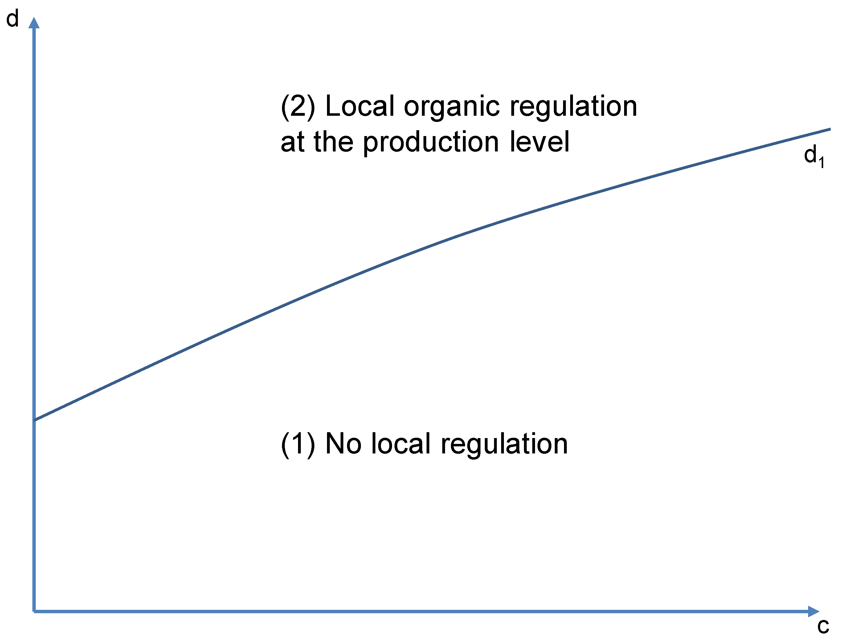
The local regulator maximizes the local welfare, accounting for the surpluses of local agents (see Appendix B for details). With damage incurred by residents and the environment close to the production site, the local policy is described in both Figure 1 and proposition 1, with the marginal cost parameter c related to the organic product represented on the x-axis and the per-unit damage d represented on the y-axis.

Proposition 1.

When local welfare is considered, the socially optimal choices are as follows: in area 1, no regulation is observed and in area 2, the regulation at the production level only impacts the local producers (proof in Appendix C).

Proposition 1 shows that the regulation depends on the relative sizes of the damage d and the cost parameters c that matter when the group that originally produced conventional products turns to innovative/organic products. The higher area is the marginal cost c of innovative products, and the lower area depicts the social benefits of having the group originally producing conventional products turn to innovative products. When the damage d is relatively low (in area 1), no regulation is useful since the distortion coming from the marginal cost c is too large compared with the size of the damage. When the damage d is relatively high, the innovative products imposed on all local producers via the regulation at the production level are optimal since this damage is fully eliminated at the local level. Nonlocal producers with conventional products continue to offer relatively cheap products to consumers. As one group of local consumers left the conventional segment, the competitive pressure on this segment is less intense for nonlocal producers who see their profit increase compared with the situation without any regulation. This effect is often overlooked by the literature, particularly on non-tariff measures. Eventually, the regulation at the consumption level is never selected, since nonlocal producers offer conventional products without any damage suffered by persons at the local level.

4.2. The Global Regulation

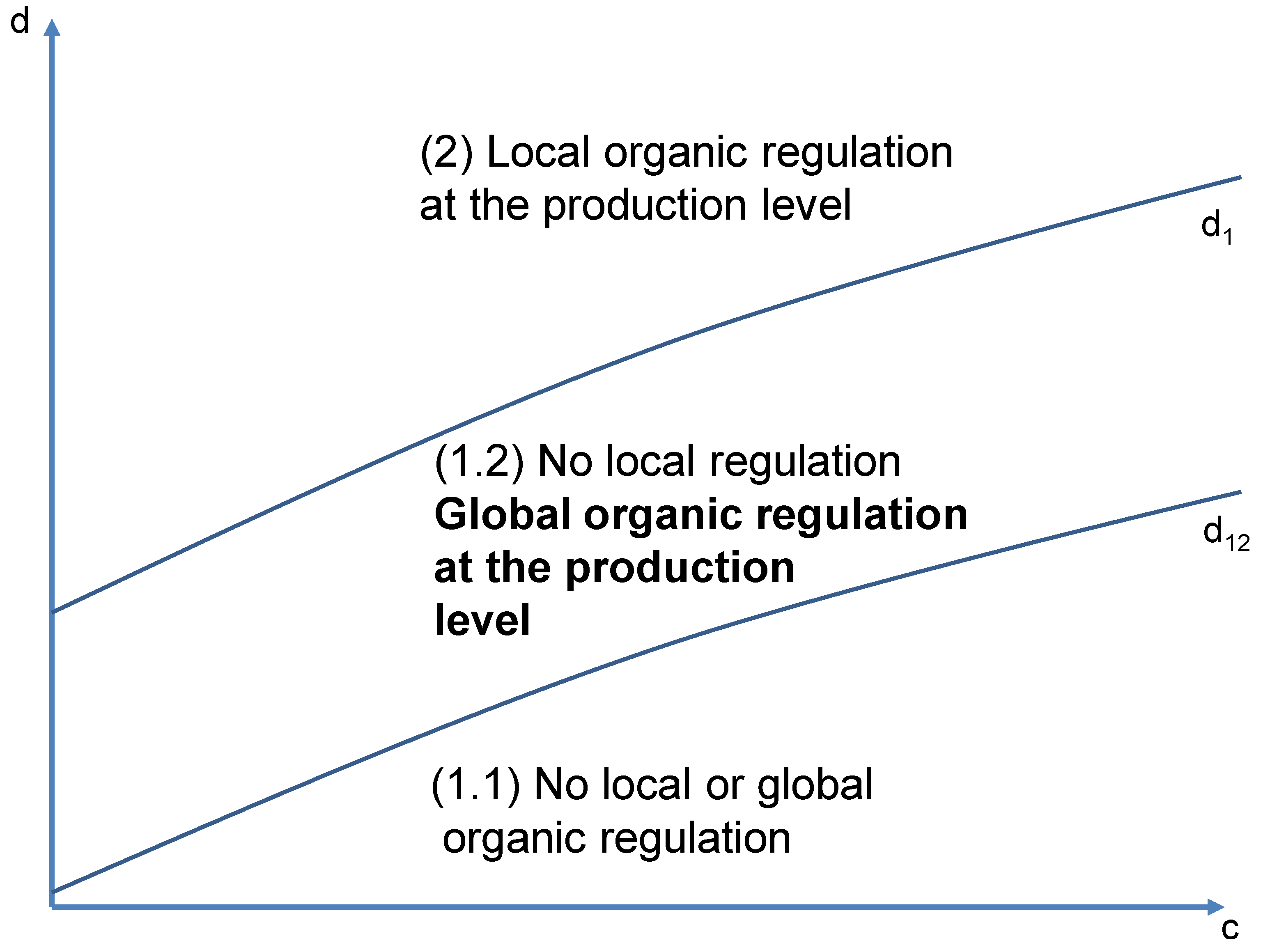
We now turn to the global policy that also includes the profits for nonlocal producers. In other words, a global regulator accounts for global welfare, including both profits and surplus for all agents, both local and nonlocal. The different welfares are compared to determine the optimal policy presented in Figure 2 and Proposition 2. Figure 2 is based on Figure 1, with the addition of the frontiers linked to global choices that could be made by a global regulator.

Proposition 2.

The choices made by the global regulator are as follows: in area 1.1, no regulation is observed; in areas 1.2 and 2, the regulation at the production level only impacts local producers; and in comparison with the local choices presented in Figure 2, global choices are different from local choices in area 1.2 (as underlined by the bold text in Figure 2) (proof in Appendix D).

Figure 2 shows that global choices made by a global regulator differ from local choices made by a local regulator. The global regulator favors regulation at the production level in areas 1.2 and 2. By including nonlocal producers, the global regulator imposes global regulation at the production level, which increases the profit of nonlocal producers. The regulation targeting the consumption level and imposing organic regulation on all producers is never selected since it would eliminate nonlocal producers. Figure 2 shows that the local regulator “underregulates” in area 1.2 compared with the global regulator, which is counterintuitive compared with debates often complaining about the excess regulation for pesticide residues. We now turn to the alternative configuration in which consumers incur the damage.

5. Welfare Analysis of Regulations When the Damage is Incurred by Consumers

5.1. The Local Regulation

With damage incurred by consumers, the local policy and results can be summarized in Figure 3 and Proposition 3.

Proposition 3.

When local welfare is considered, the socially optimal choices are: in area 3, no regulation is observed; in area 4, the regulation at the production level only impacts local producers; and in area 5, the regulation at the consumption level leads to the exclusion of nonlocal producers (proof in Appendix E).

When the damage d is relatively low (in area 3), no regulation is useful, since the distortion coming from the marginal cost c is too large compared with the size of the damage. Figure 3 shows that the two types of regulation are selected for different values of parameters when the damage d is relatively large. When the damage d is relatively medium and the marginal cost c is relatively low (in area 4), the innovative/organic products imposed on all local producers via the regulation at the production and local level are optimal since the damage is reduced. With conventional local producers turning to innovative products, the overall damage diminishes, and consumers benefit from a significant decrease in the price of innovative products because of the relatively low cost c. In area 4, the damage is reduced since nonlocal producers with conventional products implying damage for consumers are still on the market. Conversely, in area 5, the damage d becomes higher, requiring a more drastic solution compared with area 4. The regulation targeting consumption is selected, leading to the exclusion of nonlocal producers. The damage is eliminated even if some consumers suffer the absence of conventional products that were cheap in a configuration without regulation.

5.2. The Global Regulation

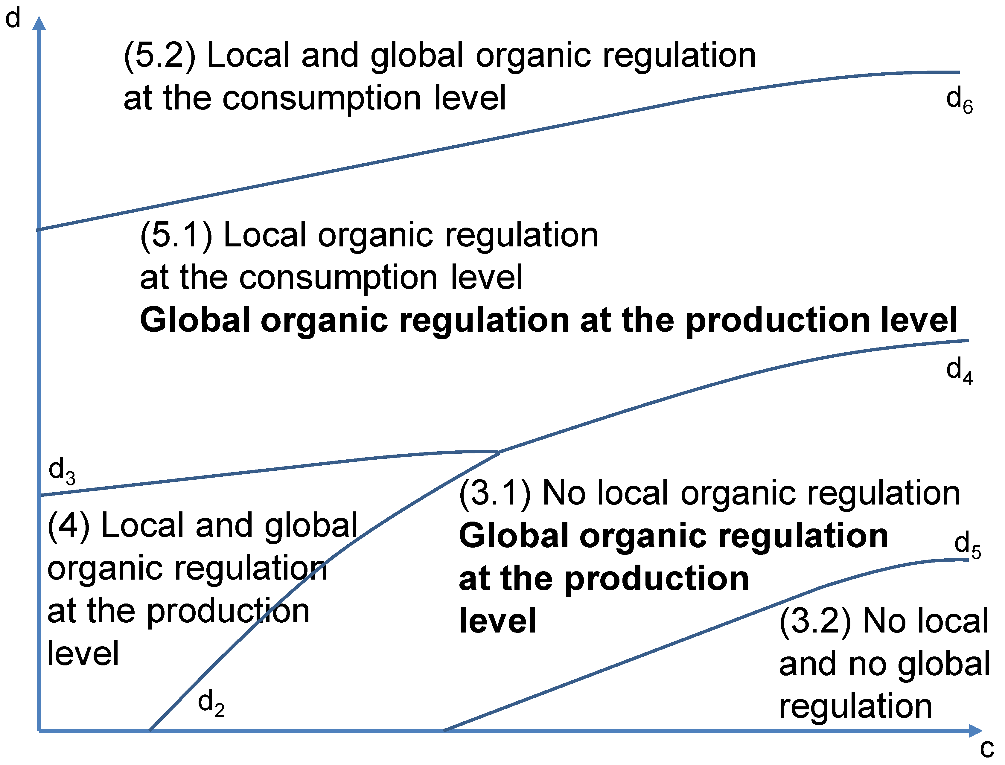
We now turn to the global policy that also includes the profits for nonlocal producers. In other words, a global regulator accounts for global welfare, including both profits and surplus for all agents, both local and nonlocal. The different welfares are compared to determine the optimal policy presented in both Figure 4 and proposition 4. Figure 4 starts from Figure 3, adding the frontiers linked to global choices that could be made by a global regulator.

Proposition 4.

The choices made by the global regulator are as follows: in area 3.2, no regulation is observed; in areas 4, 3.1, and 5.1, the regulation at the production level only impacts local producers; in area 5.2, the regulation at the consumption level leads to the exclusion of nonlocal producers; and in comparison with the local choices presented in Figure 3, global choices are different from local choices in areas 3.1 and 5.1 (as underlined by the bold text in Figure 4) (proof in Appendix F).

Figure 4 shows that global choices made by a global regulator differ from local choices made by a local regulator. The global regulator gives “more space” to the regulation at the production level. By including nonlocal producers, the global regulator tends to favor global regulation at the production level, leading to higher profits for these nonlocal producers compared with the absence of regulation. Interestingly, in comparison with the local choices presented in Figure 3, global choices are different from local choices in areas 3.1 and 5.1 (as underlined in bold in Figure 4). Figure 4 shows that the local regulator “underregulates” in area 3.1 compared with the global regulator, while this local regulator “overregulates” in area 5.1 compared with the global regulator. Figure 4 complements previous works on non-tariff measures (see references in the introduction).

6. Extensions

To identify and focus on the main economic mechanisms at work, we kept the mathematical aspects as sparse as possible by using very simple assumptions. Our analysis could accommodate various contexts using the following extensions of our model.

• In our present paper, we did not consider any demand for a country with nonlocal producers, which is an extreme assumption that corresponds to situations where there is no effective local demand, but this configuration could be introduced. In this new context, the results would be close to the results presented in this paper, even if some values of standards or frontiers in figures would change.
• In the paper, we oversimplify the regulation choice imposing 100% organic production to all producers, following the Sikkim example. However, the model can be extended less drastic objectives like a high level of organic production, representing 30%, 50%, or 60% of the production respectively, rather than the entire production. Moreover, the private incentives to adopt organic products without mandatory regulation but with clear organic labels could also be studied.
• The model focused on a single type of product with a partial equilibrium analysis, but it could be extended to several products with a general equilibrium model. This model could be also extended to several products and countries with a general equilibrium model. When several products entail a different level of per-unit damages, a new coordinate symbol E(d) representing the average damage across products may replace the original coordinate symbol d representing the damage on the longitudinal axis of the Figure 1, Figure 2, Figure 3 and Figure 4.
• The analysis here should be expanded by detailing the reaction of foreign producers to offering innovative/organic products.
• Throughout the model, we assumed that external damage does not influence market demand. However, demand and external damage can interact when consumers are aware of the damage, for example, via information [30]. Again, the results would be close to the results presented in this paper but with multiple cases, and some values of standards and frontiers in figures would change. Our results are robust if we allow for this interaction between the damage and the demand.
• In the model, we abstracted from the entry/exit of both local and nonlocal producers. When a new regulation is studied, the entry or exit of new producers could be studied. The imposition of an organic regulation requires many new investments, such as mechanical robots for weeding. These investments can be seen as sunk costs not depending on the level of production. In this case, for an organic producer with an output $q_1$ the cost function is $\frac{q_1^2}{2}+F$ with F being the sunk cost incurred for eliminating the damage. The higher F is, the lower the number of producers able to enter the organic segment is.
• This model does not take the heterogeneous production purposes of different regions into consideration. For example, the goals of organic regulation in the US and EU vary dramatically; the EU mainly intends to solve environmental problems, while the US aims to satisfy consumer preferences rather than sustainable agriculture [35]. As differences in explicit goals might bring about various degrees of influence on risk, the results based on the model would have different applicability in various regions.
• The theoretical framework can be applied to one specific food like tomatoes or apples, with empirical data to provide a quantitative cost–benefit analysis. It is possible to use an approach based on a calibrated model combining elasticities of demand obtained from times-series econometrics and average willingness-to-pay obtained from the experiment for determining monetary damage d appearing in Equations (A15) to (A26) in Appendixes [36]. For a status quo situation preceding a reinforcement of the regulation, parameters of Equation (2) can be calibrated in such a way as to replicate market prices and quantities for a given year, with the observed quantity sold over a period, the average price observed over the period, and the direct price elasticity obtained from econometric estimates [37]. When calibrated to empirically measure exchanges on one market for a given product, the partial equilibrium approach provides a welfare analysis for choosing regulatory instruments on a product-by-product basis.
• More precisely, our theoretical methodology consisted in showing that market adjustments depend on regulatory choices imposed at both local and global levels. Based on simple assumptions, this paper simply allows us to theoretically insist on the “discrepancies” between local and global regulation, which is a sensitive issue in the context of strong demand for organic products all around the world. If a comprehensive cost–benefit analysis about the development of organic agriculture is carried out in the future, the various effects theoretically underlined in this paper should be precisely taken into account in such a potential analysis, because they imply complex market adjustments at both local and global levels.

All the previous extensions should be taken into account when moving toward empirical estimations related to the implementation of local regulations imposing organic products.

7. Conclusions

Using a simplified framework focusing on local regulations and welfare risks, this paper led to new results. We showed that the local regulation imposing organic production on local producers may benefit nonlocal producers, which pleads for the development of local regulations. However, Figure 2 and Figure 4 show that global choices are different from local choices for medium values of damage, underlining possible discrepancies between local and nonlocal economic agents. These differences between local and global choices raise the question of coordination between local and global decisions for developing organic farming.

In areas where traditional agriculture seriously damages the health and production environment of residents, policymakers may establish local regulations for organic agriculture to improve. Although the local regulation of organic agriculture has played a protective role, it has brought a certain degree of damage to local and nonlocal producers. If the policymaker chooses a regulation only for local producers, it will improve the profits of nonlocal producers instead of local producers. If the policymaker chooses a regulation according to the cost of safety technology based on the damage and consumption level suffered by local consumers, it will damage the interests of nonlocal producers and benefit local producers. It can be seen that the impact of local regulation on welfare patterns is inconsistent through the two different paths of local producers and consumers. Even if the model of this paper is not directly applicable, it shows that a welfare analysis is necessary for disentangling legitimate and illegitimate non-tariff measures. Despite limitations, our paper shows that competition matters for analyzing non-tariff measures and trade.

The implications for subsequent research about this theme would consist in new empirical studies based on the theoretical analysis of this paper regarding possibilities of high levels of organic productions which might account for 50%, 60%, or 100% of the overall production. These new studies should directly tackle the nine extensions pointed out in the previous Section 6. Moreover, it is necessary to clarify the collaborative scheme between local regulation and global regulation for realizing future cost–benefit analyses.

The risks of local regulation of organic agriculture to local and nonlocal producers can be explained from the perspective of regulatory organization changes. From the dynamic organizational evolution process of local regulation, the local regulation of organic agriculture has experienced the transformation from generation to diffusion. Combined with welfare analysis, it can be seen that in the generation stage of local regulation of organic agriculture, the market of organic products is still in its infancy. Local producers need to invest sunk costs to provide organic agricultural products to the local market, while the consumers of organic agricultural products in the local market only account for a part of the public, thus bringing the risk of damage to local producers, while nonlocal producers can provide the local market with conventional agricultural products without any risk of damage. In the diffusion stage of the local regulation of organic agriculture, the market of organic products gradually matures, the preference of consumers in the local market gradually transforms into enthusiasm for organic agricultural products, the marginal sunk cost that local producers need to invest to provide organic agricultural products in the local market reduces, and the expansion of the market of organic agricultural products in the local market gradually transforms into an advantage for local producers. However, due to the change of consumers’ preference in the local market, the traditional agricultural products market of nonlocal producers has shrunk, which has gradually become unfavorable to nonlocal producers. Thus, the risk advantages and disadvantages of local regulation to local producers and nonlocal producers were staged.

References

- Fagotto, M. Sikkim, in India: The world’s first fully organic state might not be able to feed the planet, but its model is still pioneering. South China Morning Post, 18 March 2020. [Google Scholar]
- Organic without Boundaries. Sikkim—The First 100% Organic State in the World. Available online: https://www.organicwithoutboundaries.bio/2018/10/17/sikkim/ (accessed on 17 October 2018).
- Taneja, S. Sikkim Is 100% Organic! Take a Second Look—The State’s Transition to Organic Farming Is yet to Become a True Success. Available online: https://www.downtoearth.org.in/news/agriculture/organic-trial-57517 (accessed on 19 April 2017).
- Doshi, V. Sikkim’s Organic Revolution at Risk as Local Consumers Fail to Buy into Project. The Guardian. Available online: https://www.theguardian.com/global-development/2017/jan/31/sikkim-india-organic-revolution-at-risk-as-local-consumers-fail-to-buy-into-project (accessed on 31 January 2017).
- Yokessa, M.; Marette, S. A review of eco-labels and their economic impact. Int. Rev. Environ. Resour. Econ. 2019, 13, 119–163. [Google Scholar] [CrossRef]
- Hanson, J.; Dismukes, R.; Chambers, W.; Greene, C.; Kremen, A. Risk and risk management in organic agriculture: Views of organic farmers. Renew. Agric. Food Syst. 2004, 19, 218–227. [Google Scholar] [CrossRef]
- Zhang, Y.; Cao, S.; Zhang, Z.; Meng, X.; Shaping, C.; Yin, C.; Jiang, H.; Wang, S. Nutritional quality and health risks of wheat grains from organic and conventional cropping systems. Food Chem. 2020, 308, 1–8. [Google Scholar] [CrossRef] [PubMed]
- Müller, R.; Shinn, C.; Waldvogel, A.; Oehlmann, J.; Ribeiro, R.; Moreira-Santos, M. Long-term effects of the fungicide pyrimethanil on aquatic primary producers in macrophyte-dominated outdoor mesocosms in two european ecoregions. Sci. Total Environ. 2019, 665, 982–994. [Google Scholar] [CrossRef]
- Anal, A.K.; Perpetuini, G.; Petchkongkaew, A.; Tan, R.; Avallone, S.; Tofalo, R.; Nguyen, H.V.; Chu-Ky, S.; Ho, P.H.; Phan, T.T.; et al. Food safety risks in traditional fermented food from south-east Asia. Food Control 2020, 109, 1–9. [Google Scholar] [CrossRef]
- Dou, L.; Yanagishima, K.; Li, X.; Li, P.; Nakagawa, M. Food safety regulation and its implication on chinese vegetable exports. Food Policy 2015, 57, 128–134. [Google Scholar] [CrossRef]
- Toomey, E. How organic is organic—Do the USDA’s organic food production act and national organic program regulations need an overhaul. Drake J. Agric. Law 2014, 19, 127–146. [Google Scholar]
- Nie, E.; Zheng, G.; Ma, C. Characterization of odorous pollution and health risk assessment of volatile organic compound emissions in swine facilities. Atmos. Environ. 2020, 223, 1–9. [Google Scholar] [CrossRef]
- Malek, J.; Tieskens, K.F.; Verburg, P.H. Explaining the global spatial distribution of organic crop producers. Agric. Syst. 2019, 176, 102–680. [Google Scholar] [CrossRef]
- Kvakkestad, V.; Sundbye, A.; Gwynn, R.; Klingen, I. Authorization of microbial plant protection products in the scandinavian countries: A comparative analysis. Environ. Sci. Policy 2020, 106, 115–124. [Google Scholar] [CrossRef]
- María, B.A.G. The organic food sector: Regulation and ecological labeling. Pecunia Revista De La Facultad De Ciencias Económicas Y Empresariales 2016, 22, 95–119. [Google Scholar]
- Diemer, N.; Staudacher, P.; Atuhaire, A.; Fuhrimann, S.; Inauen, J. Smallholder farmers’ information behavior differs for organic versus conventional pest management strategies: A qualitative study in Uganda. J. Clean. Prod. 2020, 257, 1–9. [Google Scholar] [CrossRef]
- Calderón, R.; Palma, P.; Eltit, K.; Arancibia-Miranda, N.; Silva-Moreno, E.; Yu, W. Field study on the uptake, accumulation and risk assessment of perchlorate in a soil-chard/spinach system: Impact of agronomic practices and fertilization. Sci. Total Environ. 2020, 719, 1–7. [Google Scholar] [CrossRef] [PubMed]
- Romeis, J.; Collatz, J.; Glandorf, D.C.M.; Bonsall, M.B. The value of existing regulatory frameworks for the environmental risk assessment of agricultural pest control using gene drives. Environ. Sci. Policy 2020, 108, 19–36. [Google Scholar] [CrossRef]
- Huong, L.T.T.; Takahashi, Y.; Nomura, H.; Son, C.T.; Kusudo, T.; Yabe, M. Manure management and pollution levels of contract and non-contract livestock farming in Vietnam. Sci. Total Environ. 2020, 710, 1–11. [Google Scholar] [CrossRef]
- Luh, Y.; Tsai, M.; Fang, C. Do first-movers in the organic market stand to gain? Implications for promoting cleaner production alternatives. J. Clean. Prod. 2020, 262, 1–14. [Google Scholar] [CrossRef]
- Greenberg, M.R. Explaining Risk Analysis: Protecting Health and the Environment; Routledge Press: Abingdon, Oxon, UK, 2017. [Google Scholar]
- Baldwin, R.E. Measuring Nontariff Trade Policies; NBER Working Paper No. 2978; NBER: Cambridge, MA, USA, 1989. [Google Scholar]
- Louden, F.N.; MacRae, R.J. Federal regulation of local and sustainable food claims in canada: A case study of local food plus. Agric. Hum. Values 2010, 27, 177–188. [Google Scholar] [CrossRef]
- Muller, A.; Schader, C.; El-Hage Scialabba, N.; Brüggemann, J.; Isensee, A.; Erb, K.-H.; Smith, P.; Klocke, P.; Leiber, F.; Stolze, M.; et al. Strategies for feeding the world more sustainably with organic agriculture. Nat. Commun. 2017, 1290, 1–13. [Google Scholar] [CrossRef] [Green Version]
- Seufert, V.; Ramankutty, N.; Foley, J.A. Comparing the yields of organic and conventional agriculture. Nature 2012, 485, 229–232. [Google Scholar] [CrossRef]
- Fisher, R.; Serra, P. Standards and protection. J. Int. Econ. 2020, 52, 377–400. [Google Scholar] [CrossRef]
- Barrett, S. Strategic environmental policy and International trade. J. Public Econ. 1994, 54, 325–338. [Google Scholar] [CrossRef]
- Marette, S.; Beghin, J. Are standards always protectionist? Rev. Int. Econ. 2010, 18, 179–192. [Google Scholar] [CrossRef] [Green Version]
- Marette, S. Illegitimate or legitimate non-tariff measures. J. Agric. Food Ind. Organ. 2018, 16, 1–17. [Google Scholar] [CrossRef]
- Polinsky, A.M.; Rogerson, W.P. Products liability and consumer misperceptions and market power. Bell J. Econ. 1983, 14, 581–589. [Google Scholar] [CrossRef]
- Searchinger, D.; Wirsenius, S.; Beringer, T.; Dumas, P. Assessing the efficiency of changes in land use for mitigating climate change. Nature 2018, 564, 249–254. [Google Scholar] [CrossRef]
- Gil, Y.; Sinfort, C. Emission of pesticides to the air during sprayer application: A bibliographic review. Atmos. Environ. 2005, 39, 5183–5193. [Google Scholar] [CrossRef]
- Bajwa, U.; Sandhu, K.S. Effect of handling and processing on pesticide residues in food-a review. J. Food Sci. Technol. 2014, 51, 201–220. [Google Scholar] [CrossRef] [Green Version]
- Garella, P.; Petrakis, E. Minimum quality standards and consumers’ information. Econ. Theory 2008, 36, 283–302. [Google Scholar] [CrossRef] [Green Version]
- Klein, K.; Winickoff, D. Organic regulation across the atlantic: Emergence, divergence, convergence. Environ. Politics 2011, 20, 153–172. [Google Scholar] [CrossRef]
- Roosen, J.; Marette, S. Making the ‘right’ choice based on experiments: Regulatory decisions for food and health. Eur. Rev. Agric. Econ. 2011, 38, 361–381. [Google Scholar] [CrossRef]
- Beghin, J.; Disdier, A.C.; Marette, S.; van Tongeren, F. Measuring Costs and Benefits of Non-Tariff Measures in Agri-Food Trade. World Trade Rev. 2012, 11, 356–375. [Google Scholar] [CrossRef] [Green Version]
Figure 1.
The maximization of the local welfare with damage incurred by residents close to the production site.
Figure 2.
The maximization of the global welfare with damage incurred by residents close to the production site.
Figure 3.
The maximization of the local welfare with damage incurred by consumers.
Figure 4.
The maximization of the global welfare with damage incurred by consumers.
© 2020 by the authors. Licensee MDPI, Basel, Switzerland. This article is an open access article distributed under the terms and conditions of the Creative Commons Attribution (CC BY) license (http://creativecommons.org/licenses/by/4.0/).
Share and Cite
MDPI and ACS Style
Wu, H.; Marette, S. Local and Global Welfare When Regulating Organic Products: Should Local Regulation Target Production or Consumption? Sustainability 2020, 12, 5492. https://doi.org/10.3390/su12145492
AMA Style
Wu H, Marette S. Local and Global Welfare When Regulating Organic Products: Should Local Regulation Target Production or Consumption? Sustainability. 2020; 12(14):5492. https://doi.org/10.3390/su12145492
Chicago/Turabian StyleWu, Haijiang, and Stéphan Marette. 2020. "Local and Global Welfare When Regulating Organic Products: Should Local Regulation Target Production or Consumption?" Sustainability 12, no. 14: 5492. https://doi.org/10.3390/su12145492
Note that from the first issue of 2016, this journal uses article numbers instead of page numbers. See further details here.