Cluster Analysis of Public Bike Sharing Systems for Categorization


Department of Transport Technology and Economics, Budapest University of Technology and Economics, Stoczek utca 2, H-1111 Budapest, Hungary
*
Author to whom correspondence should be addressed.
Sustainability 2020, 12(14), 5501; https://doi.org/10.3390/su12145501
Submission received: 14 June 2020
/
Revised: 30 June 2020
/
Accepted: 3 July 2020
/
Published: 8 July 2020
(This article belongs to the Special Issue Toward Sustainability: Bike-Sharing Systems Design, Simulation and Management)
Abstract
:The world population will reach 9.8 billion by 2050, with increased urbanization. Cycling is one of the fastest developing sustainable transport solutions. With the spread of public bike sharing (PBS) systems, it is very important to understand the differences between systems. This article focuses on the clustering of different bike sharing systems around the world. The lack of a comprehensive database about PBS systems in the world does not allow comparing or evaluating them. Therefore, the first step was to gather data about existing systems. The existing systems could be categorized by grouping criterions, and then typical models can be defined. Our assumption was that 90% of the systems could be classified into four clusters. We used clustering techniques and statistical analysis to create these clusters. However, our estimation proved to be too optimistic, therefore, we only used four distinct clusters (public, private, mixed, other) and the results were acceptable. The analysis of the different clusters and the identification of their common features is the next step of this line of research; however, some general characteristics of the proposed clusters are described. The result is a general method that could identify the type of a PBS system.
1. Introduction
According to the UN forecast, the world population in mid-2017 was about 7.6 billion people, and by 2050 it is predicted to reach 9.8 billion. Along with this, urbanization is expected to increase [1,2]. Cycling is one of the fastest developing sustainable transport solutions [3,4,5,6]. Modernized and urban lifestyles have faded away physical activity of everyday life and this has resulted in a threat to population health caused by sedentary lifestyles [7]. It is estimated that physical inactivity causes 21–25% of breast and colon cancer and even greater proportions are estimated for diabetes (27%) and ischemic heart disease (30%) [8].
Public bike sharing (PBS) systems, also known as “Public-Use Bicycles”, “Bicycle Transit,” “Bikesharing”, or “Smart Bikes,” can be defined as a short-term urban bicycle rental schemes that allow bicycles to be picked up at any self-service bicycle station and returned to any other bicycle station, consisting in point-to-point trips [9]. Basically, people use bicycles on an “as-needed” basis, without the responsibility of the bicycle ownership [10]. Nowadays, different type of PBS systems start to spread all around the world, which can be operated without the docking stations, hence called dockless systems [11,12]. With the spread of public bike sharing systems, it is very important to understand the differences between systems [10,13,14,15,16]. Without understanding the differences neither the impact of these systems can be calculated, nor is high-quality decision support possible.
We developed a complete framework during a doctoral research for analyzing, comparing, and categorizing public bike sharing systems, as such a comprehensive system is still missing from the literature [17]. The first level of our framework is to collect data about existing systems and perform a cluster analysis. Then, a SWOT (strengths, weaknesses, opportunities, and threats) analysis for each cluster is compiled based on the examined systems. The third step is to create a benchmark tool, which supports the evaluation of systems. At the fourth level, impact analysis and impact assessment are carried out [18,19,20,21].
The present article deals with the clustering of different bike sharing systems around the world (i.e., it concerns the first level of our framework). The lack of a comprehensive database about PBS systems in the world does not allow for a simple comparison or evaluation of the systems [22]. Furthermore, the original goal of the creation of a PBS system is quite often unclear [23]. Without knowing the initial goal, the success of the system cannot be evaluated. A systematic literature review and scientometric analysis was conducted by Si et al. [17] from most of the bike-sharing-related articles between 2010 and 2018 from which it is clear that the researchers main focus was not on business models.
Several articles analyze the value creation of a bike sharing system [10,24,25,26], although all of them start from the assumption that there are several distinct business models for bike sharing. DeMaio [16] introduced several examples of model provision in his article, but there was no clear definition of the different models. Other articles [24,25,27,28,29] are using the business model canvas [30] approach or at least some of its elements, but these are not provide an easy to use categorization.
Our initial idea was to apply an unsupervised machine learning algorithm to a dataset, which should lead us to findings related to business models. This approach was applied in other industries like the Spanish scientific journals [31] or electric mobility [32] successfully. The cluster analysis methodology was not up to now applied in the field of PBS business models, but we collected a large dataset, which can be used to this purpose.
The goal of the clustering process is to create groups (clusters of objects) of the dataset, in a way that: (i) the objects in a given cluster are similar as much as possible; and (ii) the objects belonging to different clusters are highly different [33].The cluster analysis usually applied in the domain of spatial studies related to public bike sharing (e.g., [34,35,36,37]). In this field, the studies mostly focus on the distribution of bikes or stations.
Our main assumption is that a large proportion (i.e., 90%) of the public bike sharing systems around the world could be classified into one of the four clusters. These clusters are formulated based on the type of the owner and the type of the operator. A SWOT analysis based on this categorization could help PBS project promoters and owners to develop higher-quality systems. The clustering methodology proposed by the authors contributes, among others, to reducing a large number of primary data to several basic categories that can be treated as subjects for further analysis in the public bike sharing domain.
2. Methodology
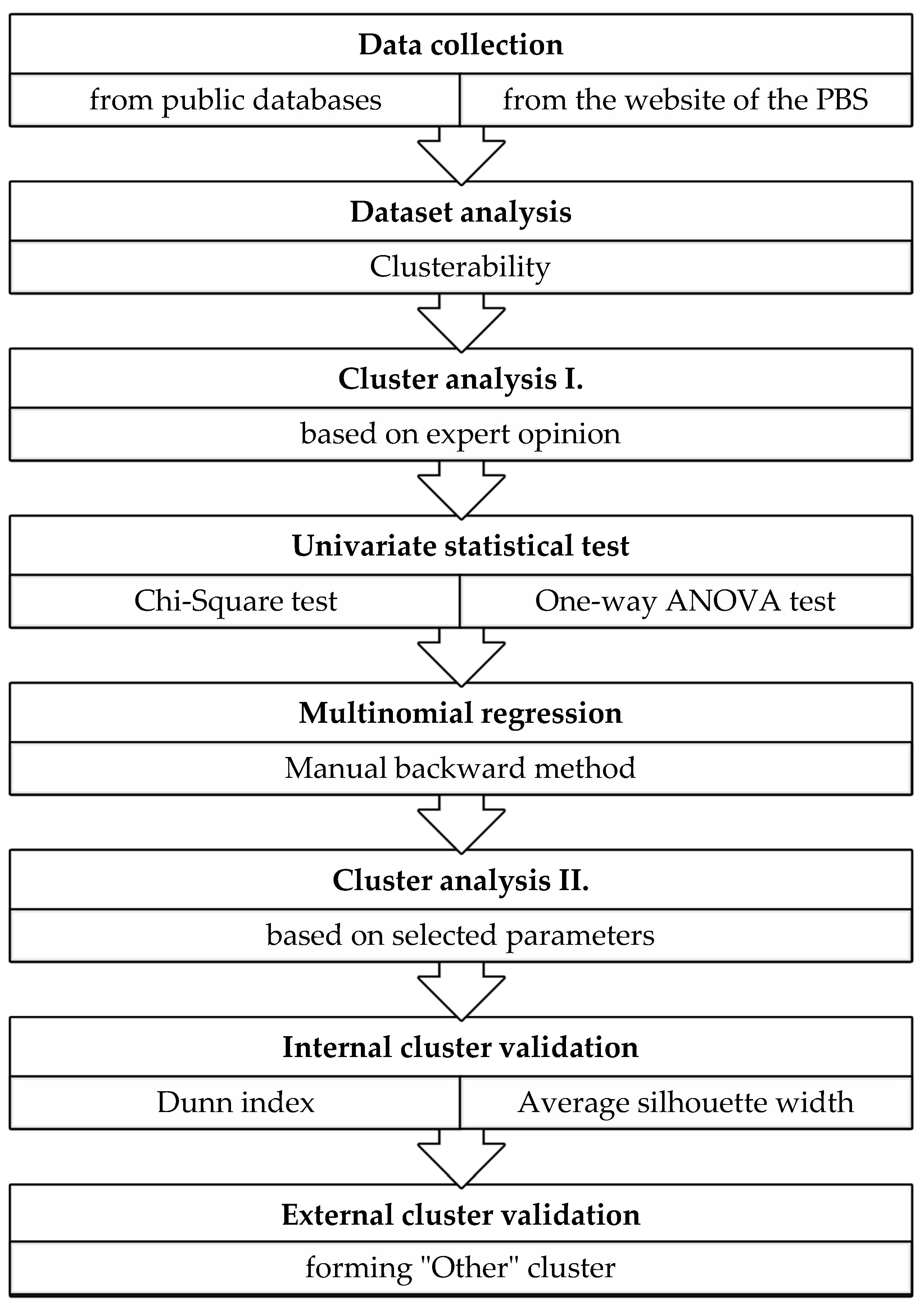
Our research followed the steps described in Figure 1.
The first step was data collection, which was followed by the initial dataset analysis. Then, the first cluster analysis based on expert opinion was conducted. The statistical tests and regression analysis were applied in order to select the parameters for the second cluster analysis. In the end, both internal and external cluster validation techniques were applied. During the analysis of the results, we compared three scenarios to each other, where different parameters were considered:
- The entire dataset (all collected 64 parameters),
- Selected parameters based on multinomial regression,
- Only operator and owner parameters.
2.1. Data Collection, Database
The original idea was to collect 80 parameters on 125 systems around the world. The collection of this data was based on open web databases and the webpages of the different bike sharing systems. We assumed that the data of the bike sharing system website are up-to-date and accurate. Our starting point was the collection of systems by Meddin [38]; this database contained 2124 active systems at the beginning of 2019. We selected the 125 systems based on the following criteria:
- 50 systems from Europe, 50 systems from Asia, 5 systems from Australia and New Zealand, and 20 systems from the Americas,
- 3/4 should be docked systems, while the remaining 1/4 is dockless.
After a 6-month-long collection period, we had to reduce the dataset to 64 systems and 64 parameters. We made the decision that to exclude the dockless systems (n = 31) from the analysis and only focus on docked bike sharing. There were several systems (n = 30) where—despite all efforts—we did not reach the minimum viable information. These systems were excluded from the analysis so as to not distort the results. Out of the originally desired 80 parameters, we had to exclude some due to the lack of available data. For example, we intended to gather information about the goals of the different systems, although it was not possible since very few system declare their initial goal, as Ricci pointed out earlier [23].
The final database was grouped around the following main topics:
- Location of the systems (Continent, Country, City, etc.),
- Contextual data (climate, start year of operation, size of the city, size of the service area, population, income, topology of the city, etc.),
- Data about the system (owner, operator, number of bikes, number of stations, etc.),
- Fare system (access fee, usage fee, deposit etc.),
- Data related to the system operations (when it is closed, how a bike can be hired, etc.),
- Derived data (bike density, station density, etc.).
2.2. Dataset Analysis
The first step was to visualize the dataset in a two-dimensional space. As the dataset itself contains several parameters, a principal component analysis (PCA) algorithm was used to reduce the number of dimensions. The algorithm presents the results in a scattered plot diagram, which gives us an easily understandable visual representation of the dataset [33].
There are several methods to calculate the distance between each pair of observations. Gower distance [39] is one of the few measures that are capable of handling both categorical and continuous variables, therefore this method was used for our calculation. The dissimilarity between two variables is the weighted mean of the contributions of each variable. This automatically implies that a particular standardization process is applied to each variable.
The daisy function from the cluster package [40] is suitable for calculating Gower distances in R. The result of computation of these distances is known as a dissimilarity matrix. The Gower distance can be described with the following Equation (1).
where is a weighted mean, is the weight, is the 0–1 weight, which becomes zero when the variable is missing in either or both rows or when the variable is asymmetric binary and both values are zero and in all other situations it is 1, and variable contribution to the total distance
We analyzed the entire dataset from the cluster tendency point of view. During the visual assessment of clustering tendency (VAT approach), we used the following steps:
- Compute the dissimilarity matrix for the data set using Gower distance.
- Reorder the dissimilarity matrix so that similar objects get close to one another, which results in an ordered dissimilarity matrix.
- The ordered dissimilarity matrix is converted into an image for visual inspection.
The color level is proportional to the value of the dissimilarity between observations. The observations in the same cluster are displayed in a consecutive order [41].
After the visual inspection, we also used the statistical method called Hopkins statistic to evaluate clusterability. This method measures the probability if a dataset was generated by a uniform distribution, so it tests the spatial randomness of the data. The calculations are the following:
- Get a random sample from the original real dataset.
- Compute a distance from each point to each nearest neighbor of the original real dataset.
- Generate a random dataset based on uniform distribution with the same variation as the original real dataset.
- Compute a distance from each point to each nearest neighbor of the random dataset.
- Calculate the Hopkins statistics (H) as the mean nearest neighbor distance in the random dataset divided by the sum of the mean nearest neighbor distance in the original real and the random dataset.
The formula of Hopkins statistics can be defined as below (2):
where H is the Hopkins statistics, yi is the nearest neighbor distance in the random dataset, xi is the nearest neighbor distance in the real dataset, and n is number of sample points in the dataset.
The null hypothesis is that the original real dataset is uniformly distributed (i.e., there are no meaningful clusters). The alternative hypothesis is that the dataset is not uniformly distributed. (i.e., there can be find meaningful clusters). If the Hopkins statistics is close to 1, we can reject the null hypothesis and conclude that there is significant clusterability. A higher than 75% value indicates a clusterability at the 90% confidence level.
2.3. Clustering Based on Expert Opinion
Our main hypothesis was that most of the PBS systems can be clustered based on the owner type and the operator type. Therefore, during data collection, we used two owner categories: Public and Private, while in the type of operator we created 4 categories: Advertising company, Private Company, Service provider, and Public. Based on these types, we created 4 clusters, which can be seen in Table 1. This categorization was based on the expert opinion of the two authors.
2.4. Univariate Statistical Tests
In order to determine which of the 64 parameters should be included in a multivariate regression model, some preselection is required [42]. As the dependent variables are both categorical and continuous, while the independent variable is categorical, we had to use two types of statistical tests. We used the SPSS statistical software for these tests.
We used the Pearson’s chi-square test to discover whether there is a relationship between two categorical variables. As all the variables were measured at an ordinal or nominal level (i.e., were categorical data) and both variables consist of at least two independent groups, the test was applicable. The null hypothesis was that Variable 1 (Cluster) is dependent from Variable 2 (all other categorical variables) [43].
We used the one-way ANOVA test to determine if there is a statistical difference between the means of independent groups and the population. The independent variable (cluster in our case) divides the dataset into mutually exclusive groups. We used this test where the dependent variables were continuous. The null hypothesis was that all group means are equal, while the alternative hypothesis was that at least one of the group means is not equal to the others. As the one-way ANOVA is an omnibus test, we do not know which of the groups are different [44].
We selected a higher significance level for both tests not to eliminate the possible candidates from the multivariate regression analysis as it was suggested by Bursac et al. (2008). If the p-value was less than our chosen significance level (), we rejected the null hypothesis, and concluded that there is an association between our two variables, therefore we selected the dependent variable for further tests [42].
2.5. Multinomial Regression
We used multinomial logistic regression to predict the nominal dependent variable (cluster of the PBS system) based on the preselected independent variables (both categorical and continuous ones). This also allows to have interaction between the independent variables to predict the dependent one. We used the SPSS statistical software for this.
The applicability of this method is based on the following assumptions:
- The dependent variable is a nominal one and should be mutually exclusive.
- There are two or more independent nominal or continuous variables.
- There should be no multicollinearity.
- There need to be a relationship between any continuous independent variable and the logit transformation of the dependent one.
- There should be no outliers.
We checked the entire dataset for the first 3 assumptions. The multicollinearity assumption was continuously tested for each different model and the rest was automatically tested in SPSS. As the software is not capable of running any automated model selection processes due to categorical variable, we decided to use the backward method and computed each step manually. First, we eliminated those independent parameters where we believed that the relationship to the dependent one would only be statistical, but there is no real reason to be related (e.g., start of operation, country etc.). Then, we added all remaining parameters to the model. We selected the variables with multicollinearity and eliminated one of them based on the significance. We reduced the model until we got a statistically significant one.
2.6. Cluster Analysis for Selected Parameters
We used a clustering method for creating associated groups from the dataset. We used the same method with different parameter sets. We decided to use a k-medoids algorithm, which belongs to the k-means clustering approaches. The most commonly used method is the partitioning around medoids (PAM) algorithm [45]. The PAM algorithm is based on the search of k representative medoids in the dataset and then it clusters the remaining dataset around them. As it does not use the means of the cluster, this method is less sensitive to outliers. The method consists of two phases: The build phase and the swap phase. In the build phase, the first step is the selection of k medoids. The second step is the calculation of the dissimilarity matrix, while the third step is the assignment of each observation into the closest medoids (therefore cluster), based on the calculated distance. In the swap phase, the fourth step is to check if swapping the current medoid of the cluster to any other object in the given cluster is reducing the average dissimilarity. If this happens, the cluster medoid should be changed to the new object and we must go back to the third step and start over again. If none of the medoids change in the fourth step the procedure stops.
2.7. Internal Cluster Validation
In order to determine how good the clustering is, we applied internal cluster validation statistics, which uses the internal information of each cluster without external data. All the different statistics measure the compactness, the separation, and the connectedness of the different clusters [40,48].
- The average distance between clusters measures the separation of clusters; as the average distance increases, so does the separation.
- The average distance within cluster objects measures the compactness of the clusters; as it decreases, the compactness increases.
- The average silhouette width also measures the separation between clusters. Each silhouette width coefficient is close to 1 if the object is in the right cluster, 0 means that the object is between clusters and −1 means that the object is entirely in the wrong cluster. So, we want the average to be as close to 1 as possible.
- The Pearson Gamma or normalized gamma coefficient shows the correlation between distances and a 01-vector where 0 means same cluster and 1 means different clusters.
- The Dunn index may be calculated in two ways, but in both cases, the Dunn index should be maximized: In the first version, the minimum separation divided by the maximum diameter; in the second way, the minimum average dissimilarity between two cluster divided by the maximum average within cluster dissimilarity.
In addition to the statistical indexes, we can also use visual methods to explore the results of clustering. The first possibility is to visualize the clusters with PCA in a two-dimensional space. The other option is the silhouette plot, where the diagram shows the silhouette coefficient for each object in an ordered way separated for each cluster.
2.8. External Cluster Validation
During the external cluster validation, we can compare two cluster validation techniques to each other. As in this research we created an expert based categorization as well as the wider parameter-based cluster using PAM method, we can compare the two categorizations to each other. The external cluster validation parameters measure how the external cluster number is matched to the clustered one.
3. Results and Discussion
The initial phase of our research was to collect the necessary data for our clustering analysis. We shared all the data which collected for this purpose online [51].
We presented the results in three different scenarios below. In the first case, we always made the assessment on the entire dataset. The second presented scenario is the one with the selected parameters based on multinomial regression. The third case is when we only use the operator and the owner parameters. We used Gower distance here as the measure of dissimilarity of the different objects.
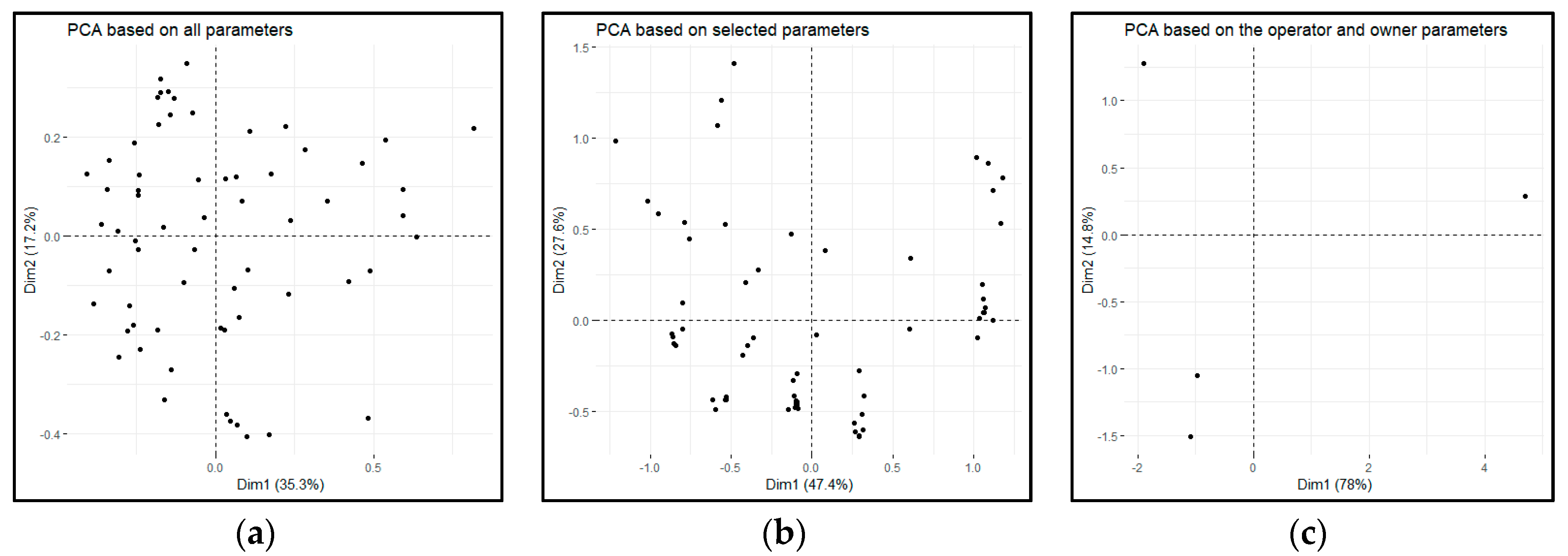
We visualized the raw dataset in a two-dimensional space using PCA methodology (Figure 2). The two axes have no specific meaning, they only provide an artificial scale for visualization purposes. Although the scaling and the axes of the figures are not the same, it is viable for comparing the resulting patterns to each other. The dataset with all parameters is less clusterable than the one with selected parameters. In the last one, only four datapoints are visible, since the entire dataset is clustered into these four points.
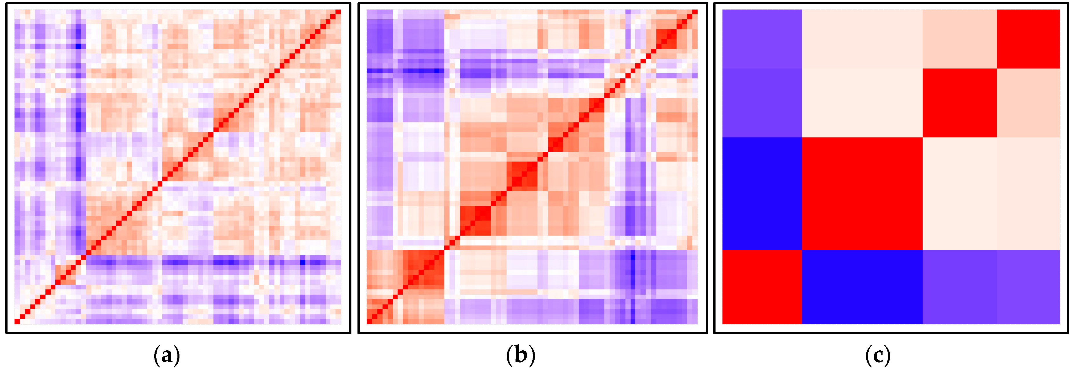
The same conclusion can be drawn from the heatmap resulting from the VAT approach (see Figure 3) as well as from the Hopkins statistics. The factoextra package [47] implements as the definition of H provided in the methodology section. Halt = 0.2661683 proved to be for all parameters (scenario 1), while Halt = 0.1565344 for the selected parameters (scenario 2). We used the seed number 123 for the calculation of Hopkins statistics.
We used the SPSS for the preselection of the parameters for the multivariate regression. Table 2 contains those variables whose p-value is lower than the chosen significance level ( in the Chi-square test.
Table 3 contains those variables whose p-value is lower than the chosen significance level ( in the one-way ANOVA test. Parameter names can be found next to the dataset description in [51].
After seven iterations with the multinomial regression, the model with the following parameters were selected:
- Factor: Int_PT_fare, Int_user_card, Wout_registration, Deposit_short, Mobile_station.
- Continuous: First_30, Agglo_coverage, Station_density, Long_aff, E_bike_density, Bikes.
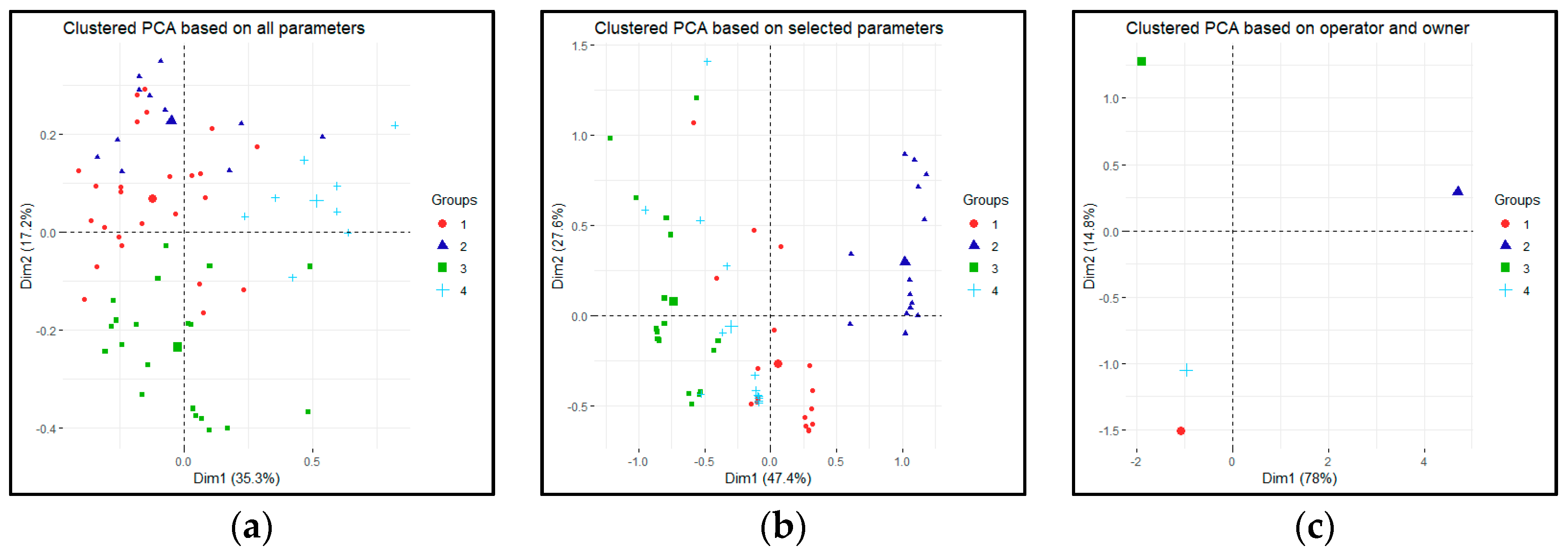
We ran the cluster analysis in the R software using the PAM method for all three scenarios with k = 4. As shown in Figure 4, the clustering is better with the selected parameters.
The results of the clustering can be described with the average silhouette width of each cluster (Table 4) and the silhouette plots Figure 5). The average silhouette width increases to 1 in the absolutely clustered scenario. The cluster based on the selected parameters has no negative data in cluster 1 and 2, which means a good clustering result.
The internal cluster validation statistics shows similar results (Table 5). Where it is appropriate, the owner and operator scenario has the theoretical minimum or maximum values. There are some exceptions e.g., the first Dunn index shows worse results for the selected parameter scenario than the all-parameters one.
External cluster validation was based on the clustering related to the expert opinion. Therefore, the last column of Table 6 is just for reference purposes; obviously, it has no meaning besides that the statistical calculation is working.
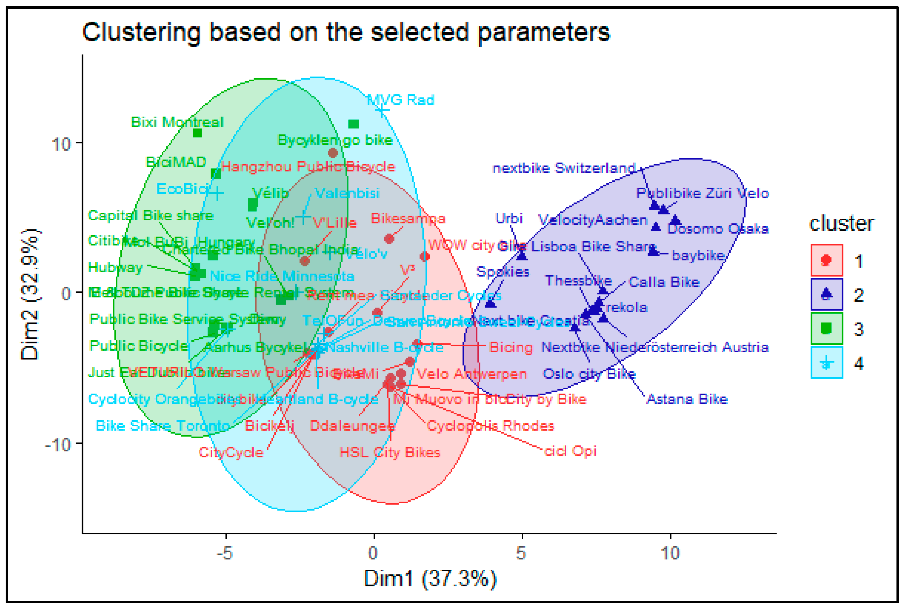
The results of the clustering algorithm for the selected parameter can be seen in Figure 6. There is a distinct cluster which is clearly different from the others, while the remaining three are somewhat overlapping.
We compared expert-based clustering with parameter-based clustering. Out of 64 systems, 42 clustered into the same cluster as the expert based method suggests and the remaining 22 (35%) were misplaced by the clustering algorithm. Based on our results, we decided that these 22 systems should be categorized as a fifth cluster, called Other. The clustering was correct for the systems, which were owned by a private company: No system with such parameters was missing, and none was misplaced to this cluster. The public systems showed similarly good results, as there were only 3 out of 12 that were misplaced and even these 3 showed some similarity with the selected clusters (e.g., Bixi Montreal is a public system, but has similarity with a commercial one, the two others were Chinese systems, where the difference between a public or a private company is sometimes hard to spot).
Eleven systems were misplaced into the cluster where the operator is supposed to be an advertising company, although all these systems are operated by a service provider. It was also true for the other way around: Four systems out of five were misplaced into the cluster with a service provider as operator, although they have an advertising company operator. This might indicate that the service provider and the advertising company business model and those system characteristics are not as distinct from each other as the purely public and purely private models.
If we only use three big clusters (purely public, purely private, and mixed), we end up only with the miscategorization of 6 systems out of 64. The analysis of the different clusters and the identification of their common features is the next step of this line of research, however some general characteristics of the proposed four clusters can be described here as a starting point. The basis of these descriptions is both the categorization described in Section 2.3 and the results of the clustering exercise:
- Cluster 1 (Public systems): Both the operator and owner of the system are public institutions. The owner is usually a city or one of its companies. The operator can be the same organization or a new one created for this specific purpose. The income is coming directly from the user fees, but usually it requires subsidization. The goal of such a scheme usually is to provide an alternative transport mode or educate the citizens rather than profit making. Typical example: MVG Rad (Munich).
- Cluster 2 (Private systems): Both the operator and owner of the system are private companies, usually the same one. The income is coming from the user fees as well as advertisements. The goal here is clearly profit making, therefore a more cost-efficient operation is envisaged. Furthermore, some limitation related to the network or the users can be applied. Typical example: NextBike Croatia.
- Cluster 3 (Mixed systems): The owner of the system is a public entity (usually a city or a transport operator), while the operator is a private company. The goal of the owner is usually to provide wider transport choices to citizens, while a private company is providing a service. There are two distinct business models for the private company based on the main source of income. In both cases, the user fees are collected for the owner, hence the financial risk from the usage is on the owner side. In the first type, the service provider gets a service fee (availability payment) based on a service level agreement. In the second type, the operator can use different advertising spaces around the city to cover the expenses of the system operation. However, from the system point of view, there are not enough distinct features of these two subtypes to cluster them separately. Typical example: MOL-Bubi (Budapest-subtype 1); Velib (Paris-subtype 2).
- Cluster 4 (other systems): There are several systems that can be categorized by an unsupervised algorithm to one of the above clusters based on the expert knowledge of the authors cannot fit well with them. The reasons are usually hard to spot, but for instance, it can be that a public company design a system with clear profit-making goals, or a private company acts similarly towards a public entity. There are especially some outliers in the Chinese systems, due to the specificities of the country political structure.
Additionally, there are some limitations with the current methodology. As it was stated above, collecting all parameters from the different systems is a time-consuming process. Furthermore, the current data become outdated very quickly as not only new systems emerge, but also the technology changes. This research does not consider dockless schemes, although they have become more and more popular in recent years [52]. At the same time, these systems are almost all profit-oriented, privately funded systems, which can be easily put under the same, distinct category. The other problem with this type of applied, data-driven approach is that an error in data collection can cause problems in interpreting the results. This was one of the reasons that we chose a clustering method that is less vulnerable to outliers.
4. Conclusions
In this study, we developed a method for categorizing public bike sharing systems, which consisted of 8 steps:
- Data collection,
- Dataset analysis,
- Cluster analysis I.,
- Univariate statistical tests,
- Multinomial regression,
- Cluster analysis II.,
- Internal cluster validation,
- External cluster validation.
During data collection, we faced several problems, therefore only 64 parameters were collected from 64 systems around the world [51]. The dataset analysis showed that the dataset is clusterable. We selected the operator and owner type as initial parameters for expert based clustering, from which we created four clusters.
We preselected 19 factor type and 15 continuous type parameters for multinomial regression, based on the univariate statistical tests, out of which five factor parameters and six continuous parameters were selected for the final model.
We reran the PAM-approach-based clustering again with the selected parameters, which resulted in better fit than in the case of all parameters. Forty-two systems were assigned to the correct clusters, the remaining 22 were misplaced by the clustering algorithm. Our initial assumption was too optimistic, as only 65% of the systems could be clustered with this method. Thirty-five percent fall into the “Other” category. At the same time, if we only use three main clusters (public, private, and mixed), the error is reduced to 6 systems out of 64.
This can be arguably a correct solution as the service provider and the advertising company business model might not be separated. So, there are four proposed clusters: Public systems, private systems, mixed systems, and other systems.
This article describes the basic characteristics of these clusters, however analyzing the characteristics in details of the different clusters is the next step of this ongoing research. Additionally, future research work will be devoted to overcoming some of the limitations of the presented methodology. One of the main limitations is the data availability; if new, reliable data become available (e.g., usage data, travel pattern, financial data), the current methodology can be expanded to cover this. Another development path can be the inclusion of the dockless schemes to the current analysis, which was neglected in this article due to the lack of reliable data.
This article can help for those who would like to apply the clustering methodology in a different domain. At the same time, it can provide a basis for further research in the public bike sharing domain, as the proposed methodology can be applied for a different set of PBS systems. A newly designed system can be categorized based on the owner and operator, which can help to find similar systems and identify problems and best practices in the earl stage. In other words, this paper can provide significant added value for researchers and academics as well as policy makers and practitioners.
Author Contributions
Conceptualization T.M. and J.T.; methodology T.M. and J.T.; writing—original draft preparation T.M. and J.T.; writing—review and editing, T.M. and J.T.; visualization, T.M.; supervision, J.T. All authors have read and agreed to the published version of the manuscript.
Funding
This research received no external funding.
Conflicts of Interest
The authors declare no conflict of interest.
References
- United Nations, Department of Economic and Social Affairs Population Division. World Population Prospects The 2012 Revision Volume I: Comprehensive Tables; (ST/ESA/SER.A/336); United Nations, Department of Economic and Social Affairs: New York, NY, USA, 2013. [Google Scholar]
- United Nations, Department of Economic and Social Affairs; Population Division. World Urbanization Prospects: The 2018 Revision; (ST/ESA/SER.A/420); United Nations, Department of Economic and Social Affairs: New York, NY, USA, 2019. [Google Scholar]
- Fenton, B.; Nash, A.; Wedderburn, M. Walking, Cycling and Congestion—Implementer’s Guide to Using the FLOW Tools for Multimodal Assessments; FLOW Consortium: Brussels, Belgium, 2018. [Google Scholar]
- Rudolph, F.; Mátrai, T. Congestion from a Multimodal Perspective. Period. Polytech. Transp. Eng. 2018, 46, 215–221. [Google Scholar] [CrossRef] [Green Version]
- Szabó, Z.; Török, Á. Spatial Econometrics—Usage in Transportation Sciences: A Review Article. Period. Polytech. Transp. Eng. 2019. [Google Scholar] [CrossRef]
- Pupavac, D.; Maršanić, R.; Krpan, L. Elasticity of Demand in Urban Traffic Case Study: City of Rijeka. Period. Polytech. Transp. Eng. 2019. [Google Scholar] [CrossRef]
- Garrard, J. Active Transport: Children and Young People, An Overview of Recent Evidence; Vic Health: Melbourne, VI, Australia, 2009.
- World Health Organization. Global Health Risks: Mortality and Burden of Disease Attributable to Selected Major Risks; World Health Organization: Geneva, Switzerland, 2009. [Google Scholar]
- Department for City Planning New York. Bike-Share—Opportunities in New York City; Department for City Planning New York: New York, NY, USA, 2009.
- Shaheen, S.; Guzman, S.; Zhang, H. Bikesharing in Europe, the Americas, and Asia: Past, Present, and Future. Transp. Res. Rec. J. Transp. Res. Board 2010, 2143, 159–167. [Google Scholar] [CrossRef] [Green Version]
- Luo, H.; Kou, Z.; Zhao, F.; Cai, H. Comparative life cycle assessment of station-based and dock-less bike sharing systems. Resour. Conserv. Recycl. 2019. [Google Scholar] [CrossRef]
- Fishman, E. Bikeshare: A Review of Recent Literature. Transp. Rev. 2016, 36, 92–113. [Google Scholar] [CrossRef]
- Shaheen, S.A.; Martin, E.W.; Chan, N.D. Public Bikesharing in North America: Early Operator and User Understanding, MTI Report 11-19. Mineta Transp. Inst. Publ. 2012. [Google Scholar] [CrossRef]
- Fishman, E.; Washington, S.; Haworth, N. Barriers and facilitators to public bicycle scheme use: A qualitative approach. Transp. Res. Part F Traffic Psychol. Behav. 2012, 15, 686–698. [Google Scholar] [CrossRef] [Green Version]
- Fishman, E.; Washington, S.; Haworth, N. Bike Share: A Synthesis of the Literature. Transp. Rev. 2013, 33, 148–165. [Google Scholar] [CrossRef] [Green Version]
- DeMaio, P. Bike-Sharing: History, Impacts, Models of Provision, and Future. J. Publ. Transp. 2009, 12, 41–56. [Google Scholar] [CrossRef]
- Wu, G.; Si, H.; Chen, J.; Shi, J.; Zhao, X. Mapping the bike sharing research published from 2010 to 2018: A scientometric review. J. Clean. Prod. 2018, 213, 415–427. [Google Scholar] [CrossRef]
- Mátrai, T.; Tóth, J. Comparative Assessment of Public Bike Sharing Systems. Transp. Res. Procedia 2016, 14, 2344–2351. [Google Scholar] [CrossRef] [Green Version]
- Tóth, J.; Mátrai, T. Újszerű, nem motorizált közlekedési megoldások. In Proceedings of the Közlekedéstudományi Konferencia, Győr, Hungary, 26–27 March 2015. [Google Scholar]
- Mátrai, T.; Mándoki, P.; Tóth, J. Benchmarking tool for bike sharing systems. In Proceedings of the Third International Conference On Traffic And Transport Engineering (ICTTE), Belgrade, Serbia, 24–25 November 2016; Cokorilo, O., Ed.; Scientific Research Center Ltd.: Belgrade, Serbia; pp. 550–558.
- Mátrai, T.; Tóth, J. Categorization of bike sharing systems: A case study from Budapest. In Proceedings of the European Conference on Mobility Management, Athens, Greece, 1–3 June 2016. [Google Scholar]
- Médard de Chardon, C. The contradictions of bike-share benefits, purposes and outcomes. Transp. Res. Part A Policy Pract. 2019, 121, 401–419. [Google Scholar] [CrossRef]
- Ricci, M. Bike sharing: A review of evidence on impacts and processes of implementation and operation. Res. Transp. Bus. Manag. 2015, 15, 28–38. [Google Scholar] [CrossRef]
- Winslow, J.; Mont, O. Bicycle Sharing: Sustainable Value Creation and Institutionalisation Strategies in Barcelona. Sustainability 2019, 11, 728. [Google Scholar] [CrossRef] [Green Version]
- Cohen, B.; Kietzmann, J. Ride On! Mobility Business Models for the Sharing Economy. Organiz. Environ. 2014, 27, 279–296. [Google Scholar] [CrossRef]
- Hamidi, Z.; Camporeale, R.; Caggiani, L. Inequalities in access to bike-and-ride opportunities: Findings for the city of Malmö. Transp. Res. Part A Policy Pract. 2019, 130, 673–688. [Google Scholar] [CrossRef]
- Zhang, L.; Zhang, J.; Duan, Z.; Bryde, D. Sustainable bike-sharing systems: Characteristics and commonalities across cases in urban China. J. Clean. Prod. 2015, 97, 124–133. [Google Scholar] [CrossRef]
- Van Waes, A.; Farla, J.; Frenken, K.; de Jong, J.P.J.; Raven, R. Business model innovation and socio-technical transitions. A new prospective framework with an application to bike sharing. J. Clean. Prod. 2018, 195, 1300–1312. [Google Scholar] [CrossRef]
- Gao, P.; Li, J. Understanding sustainable business model: A framework and a case study of the bike-sharing industry. J. Clean. Prod. 2020, 267, 122229. [Google Scholar] [CrossRef]
- Osterwalder, A.; Pigneur, Y.; Tucci, C.L. Clarifying Business Models: Origins, Present, and Future of the Concept. Commun. Assoc. Inform. Syst. 2005, 16, 1. [Google Scholar] [CrossRef] [Green Version]
- Claudio-González, M.G.; Martín-Baranera, M.; Villarroya, A. A cluster analysis of the business models of Spanish journals. Learn. Publ. 2016, 29, 239–248. [Google Scholar] [CrossRef]
- Engel, C.; Haude, J.; Kühl, N. Business Model Clustering: A network-based approach in the field of e-mobility services. In Proceedings of the 2nd Karlsruhe Service Summit, Karlsruhe, Germany, 25–26 February 2016; pp. 11–25. [Google Scholar]
- Kassambara, A. Practical Guide to Cluster Analysis in R: Unsupervised Machine Learning, 1st ed.; STHDA: Marseille, France, 2017; ISBN 1542462703. [Google Scholar]
- Boufidis, N.; Nikiforiadis, A.; Chrysostomou, K.; Aifadopoulou, G. Development of a station-level demand prediction and visualization tool to support bike-sharing systems’ operators. Transp. Res. Procedia 2020, 47, 51–58. [Google Scholar] [CrossRef]
- Wei, X.; Luo, S.; Nie, Y.M. Diffusion behavior in a docked bike-sharing system. Transp. Res. Part C Emerg. Technol. 2019, 107, 510–524. [Google Scholar] [CrossRef]
- Jia, W.; Tan, Y.; Liu, L.; Li, J.; Zhang, H.; Zhao, K. Hierarchical prediction based on two-level Gaussian mixture model clustering for bike-sharing system. Knowl. Based Syst. 2019, 178, 84–97. [Google Scholar] [CrossRef]
- Kou, Z.; Cai, H. Understanding bike sharing travel patterns: An analysis of trip data from eight cities. Phys. A Stat. Mech. Appl. 2019. [Google Scholar] [CrossRef]
- Meddin, R. Bike Sharing Map. Available online: www.bikesharingmap.com (accessed on 28 February 2020).
- Gower, J.C. A General Coefficient of Similarity and Some of Its Properties. Biometrics 1971, 27, 857. [Google Scholar] [CrossRef]
- Maechler, M.; Rousseeuw, P.; Struyf, A.; Hubert, M.; Hornik, K. Cluster: Cluster Analysis Basics and Extensions, R Package version 2.0.8; R Core Team: Vienna, Austria, 2019. [Google Scholar]
- Bezdek, J.C.; Hathaway, R.J. VAT: A tool for visual assessment of (cluster) tendency. In Proceedings of the International Joint Conference on Neural Networks, Honolulu, HI, USA, 12–17 May 2002; pp. 2225–2230. [Google Scholar] [CrossRef]
- Bursac, Z.; Gauss, C.H.; Williams, D.K.; Hosmer, D.W. Purposeful selection of variables in logistic regression. Sour. Code Biol. Med. 2008, 3. [Google Scholar] [CrossRef] [Green Version]
- Yeager, K. SPSS Tutorials: Chi-Square Test of Independence. Available online: https://libguides.library.kent.edu/SPSS/ChiSquare (accessed on 31 August 2019).
- Yeager, K. SPSS Tutorials: One-Way ANOVA. Available online: https://libguides.library.kent.edu/spss/onewayanova (accessed on 31 August 2019).
- Kaufman, L.; Rousseeuw, P.J. Finding Groups in Data: An Introduction to Cluster Analysis; Wiley Series in Probability and Statistics; John Wiley & Sons, Inc.: Hoboken, NJ, USA, 1990; ISBN 9780470316801. [Google Scholar]
- R Core Team. R: A Language and Environment for Statistical Computing; R Core Team: Vienna, Austria, 2017. [Google Scholar]
- Kassambara, A.; Fabian, M. Factoextra: Extract and Visualize the Results of Multivariate Data Analyses; STHDA: Marseille, France, 2017. [Google Scholar]
- Halkidi, M.; Batistakis, Y.; Vazirgiannis, M. On clustering validation techniques. J. Intel. Inform. Syst. 2001, 17, 107–145. [Google Scholar] [CrossRef]
- Gordon, A.D. Classification; Chapman and Hall: London, UK; CRC: Boca Raton, FL, USA, 1999; ISBN 9780367805302. [Google Scholar]
- Meilǎ, M. Comparing clusterings-an information based distance. J. Multivar. Anal. 2007, 98, 873–895. [Google Scholar] [CrossRef] [Green Version]
- Mátrai, T. Public bike sharing systems database. Mendeley Data 2019. [Google Scholar] [CrossRef]
- Caggiani, L.; Camporeale, R.; Ottomanelli, M.; Szeto, W.Y. A modeling framework for the dynamic management of free-floating bike-sharing systems. Transp. Res. Part C Emerg. Technol. 2018, 87, 159–182. [Google Scholar] [CrossRef]
Figure 1.
Flow-chart for the cluster analysis.

Figure 2.
Dataset visualized with principal component analysis (PCA) (a) based on all parameters; (b) based on the selected parameters; (c) based on the operator and owner parameters.
Figure 2.
Dataset visualized with principal component analysis (PCA) (a) based on all parameters; (b) based on the selected parameters; (c) based on the operator and owner parameters.

Figure 3.
Visualization of the dissimilarity matrix (a) based on all parameters; (b) based on the selected parameters; (c) based on the operator and owner parameters.
Figure 3.
Visualization of the dissimilarity matrix (a) based on all parameters; (b) based on the selected parameters; (c) based on the operator and owner parameters.

Figure 4.
Clustered dataset visualized with PCA (a) based on all parameters; (b) based on the selected parameters; (c) based on the operator and owner parameters.
Figure 4.
Clustered dataset visualized with PCA (a) based on all parameters; (b) based on the selected parameters; (c) based on the operator and owner parameters.

Figure 5.
Silhouette plot for clustering (a) based on all parameters; (b) based on the selected parameters; (c) based on the operator and owner parameters.
Figure 5.
Silhouette plot for clustering (a) based on all parameters; (b) based on the selected parameters; (c) based on the operator and owner parameters.

Figure 6.
Clustering visualized with PCA based on the selected parameters.


Table 1.
Clustering logic based on the operator and the owner.
| Cluster Number | Owner | Operator | Comment |
|---|---|---|---|
| 1 | Public | Advertising company | An advertising company provides services to a public institution, the income for the advertising company might not be realized from the direct user fees, but from some advertising spaces around the city |
| 3 | Public | Service provider | A service provider operates a system on behalf of the public institution, the income for these service providers can be an availability payment. |
| 4 | Public | Public | A public institution operates the system or sets up a public company for operation, the income is directly from the user fees. |
| 2 | Private | Private company | The owner of the system is the same private company as the operator, the incomes are from the user fees and from the advertisements. |
Table 2.
Results of the Chi-square tests.
| Parameter | Value | Asymptotic Significance (2-Sided) |
|---|---|---|
| Owner | 63.574 | 0.000 |
| Operator | 183.798 | 0.000 |
| User_card_dock | 15.654 | 0.001 |
| Wout_registration | 12.026 | 0.007 |
| User_card_terminal | 11.718 | 0.008 |
| Int_user_card | 11.156 | 0.011 |
| Deposit_short | 11.148 | 0.011 |
| Continent | 19.562 | 0.021 |
| Credit_card_terminal | 9.109 | 0.028 |
| Mobile_station | 8.045 | 0.045 |
| App_bike | 7.999 | 0.046 |
| Country | 126.487 | 0.051 |
| Hour_closed | 6.995 | 0.072 |
| Diff_station | 19.487 | 0.077 |
| Code_dock | 6.133 | 0.105 |
| Code_terminal | 6.106 | 0.107 |
| Diff_renting_option | 25.603 | 0.109 |
| Deposit_long | 6.050 | 0.109 |
| Int_PT_Fare | 5.415 | 0.144 |
| Code_bike | 4.287 | 0.232 |
Table 3.
Results of the one-way ANOVA tests.
| Parameter | F | Significance |
|---|---|---|
| Operation | 13.773 | 0.000 |
| Deposit_short_EUR | 4.367 | 0.007 |
| Service_area | 3.877 | 0.013 |
| Deposit_long_EUR | 3.793 | 0.014 |
| E_bikes_dens | 3.686 | 0.016 |
| Station | 3.433 | 0.022 |
| Bikes | 3.365 | 0.024 |
| Docks | 3.141 | 0.031 |
| City_size | 2.337 | 0.082 |
| Population | 2.096 | 0.109 |
| Long_att | 1.884 | 0.142 |
| Long_aff | 1.818 | 0.154 |
| First_30 | 1.776 | 0.160 |
| Agglo_coverage | 1.555 | 0.209 |
| Station_density | 1.449 | 0.237 |
Table 4.
Cluster size and average silhouette width in three different scenarios.
| Cluster Id. | Based on All Parameters | Based on the Selected Parameters | Based on the Operator and Owner Parameters | |||
|---|---|---|---|---|---|---|
| Cluster Size | Average Silhouette Width | Cluster Size | Average Silhouette Width | Cluster Size | Average Silhouette Width | |
| 1 | 25 | 0.04 | 19 | 0.33 | 14 | 1 |
| 2 | 11 | 0.10 | 15 | 0.60 | 15 | 1 |
| 3 | 20 | 0.12 | 17 | 0.22 | 23 | 1 |
| 4 | 8 | 0.17 | 13 | 0.24 | 12 | 1 |
Table 5.
Internal cluster validation statistics for the three different alternatives.
| Based on All Parameters | Based on the Selected Parameters | Based on the Operator and Owner Parameters | |
|---|---|---|---|
| Number of observations | 64 | 64 | 64 |
| Average distance between clusters | 0.2543182 | 0.330922 | 0.7448368 |
| Average distance within cluster | 0.2315138 | 0.1898745 | 0 |
| Average silhouette width | 0.01317239 | 0.356468 | 1 |
| Pearson Gamma coefficient | 0.1585032 | 0.4660481 | 0.8330978 |
| Dunn index, first version | 0.2005322 | 0.1838311 | ∞ |
| Dunn index, second version | 0.8049529 | 1.323103 | ∞ |
Table 6.
External cluster validation statistics for the three different alternatives.
| Based on All Parameters | Based on the Selected Parameters | Based on the Operator and Owner Parameters | |
|---|---|---|---|
| Corrected Rand index | 0.07757761 | 0.4368271 | 1 |
| Variation Index | 2.22212 | 1.217804 | 4.440892 × 10⁻¹⁶ |
© 2020 by the authors. Licensee MDPI, Basel, Switzerland. This article is an open access article distributed under the terms and conditions of the Creative Commons Attribution (CC BY) license (http://creativecommons.org/licenses/by/4.0/).
Share and Cite
MDPI and ACS Style
Mátrai, T.; Tóth, J. Cluster Analysis of Public Bike Sharing Systems for Categorization. Sustainability 2020, 12, 5501. https://doi.org/10.3390/su12145501
AMA Style
Mátrai T, Tóth J. Cluster Analysis of Public Bike Sharing Systems for Categorization. Sustainability. 2020; 12(14):5501. https://doi.org/10.3390/su12145501
Chicago/Turabian StyleMátrai, Tamás, and János Tóth. 2020. "Cluster Analysis of Public Bike Sharing Systems for Categorization" Sustainability 12, no. 14: 5501. https://doi.org/10.3390/su12145501
Note that from the first issue of 2016, this journal uses article numbers instead of page numbers. See further details here.