


Introduction
Since the early days of geomorphology, it has been known that valleys carved by glaciers are U-shaped, as opposed to valleys carved by rivers which are V-shaped (Campbell, Reference Campbell1865; McGee, Reference McGee1894). Focusing on the former, it is intuitive that following step by step the detailed erosion process of the valley walls and glacier bed through time requires many assumptions and details. This process can be modelled numerically (e.g. Harbor, Reference Harbor1995; Seddik and others, Reference Seddik, Greve and Sugiyama2009; Yang and Shi, Reference Yang and Shi2015). However, it is simpler to describe the final product of the glacier action, which can be done with an analytical approach first proposed by Hirano and Aniya (Reference Hirano and Aniya1988). From the phenomenological point of view, crude models of transverse glacial valley profiles used parabolas (Svensson, Reference Svensson1959) or power-law profiles, but there was no theory behind this so-called ‘power-flaw’, which amounted to mere data-fitting (Pattyn and Van Huele, Reference Pattyn and Van Huele1998).
The Hirano and Aniya (Reference Hirano and Aniya1988) approach (refined by Morgan (Reference Morgan2005)) uses a variational principle in which the friction of the ice against the valley walls, which is a functional of the transverse profile of the glacial valley, is extremized subject to an appropriate constraint. To fix the geometry, denote with x ∈ ( − x 0, x 0) a coordinate transverse to the glacier flow, while the margins of the ice have coordinates ±x 0. Let the ice thickness at x be H(x). Correspondingly, the profile of the glacial valley is given by the bed elevation B(x) = H s − H(x), where the constant H s denotes the maximum ice thickness reached at x = 0 (see Fig. 1).
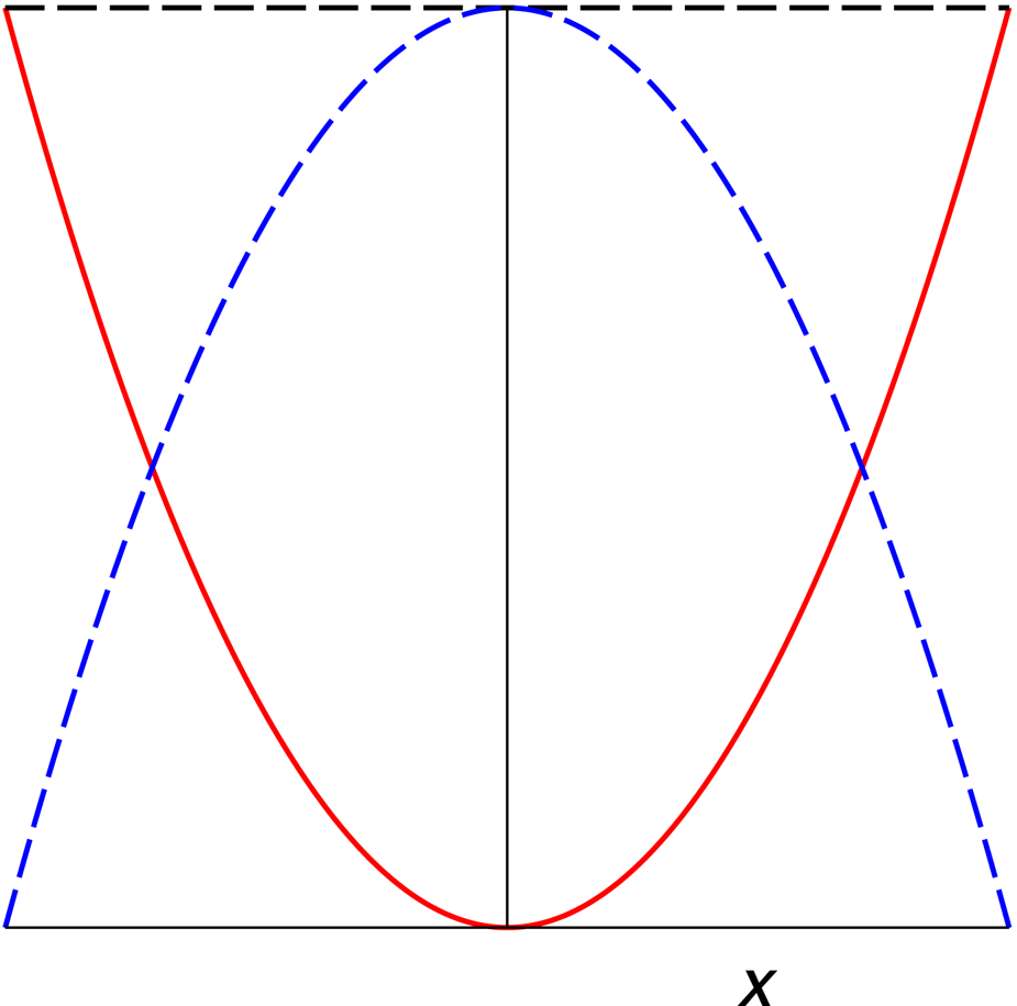
Fig. 1. The glacial valley is contained between −x 0 and x 0, the ice thickness (blue, dashed curve) is H(x) and is maximum at x = 0, where H = H s. The bed elevation (red, solid curve) over the deepest point in the ice (valley profile) is B(x) = H s − H(x).
As is clear from Figure 1, the cross-sectional area of the valley is

and the friction force is modelled by Coulomb's law,

where N = ρ icegHA contact is the normal force caused by the cryostatic pressure, μ is the friction coefficient, ρ ice is the ice density, g is the acceleration of gravity, and A contact is the area of contact between the ice and the wall.
A word of caution about the assumptions of the Hirano–Aniya–Morgan theory is mandatory. The friction model may not be entirely appropriate, since friction could depend on the velocity and the Coulomb law adopted in this theory could be an oversimplification. Indeed, friction is taken to depend on the velocity in the numerical simulations of the dynamical development of glacial valley profiles of Seddik and others (Reference Seddik, Greve and Sugiyama2009).
Moreover, because normal stress should be used in the calculation of friction, the assumption of hydrostatic pressure may fail outside of the shallow ice approximation. It is possible that the model stretches the validity of its assumptions, but since the shallow ice approximation holds well for so many valley glaciers and is required extensively in glacier modelling anyway, perhaps this is not a big issue.
A second potential problem is that glacier hydrology is neglected in the Hirano–Aniya–Morgan scenario. Hirano and Aniya (Reference Hirano and Aniya1988, Reference Hirano and Aniya1990, Reference Hirano and Aniya2005) mention that the effective pressure may not be entirely cryostatic but proceeds by assuming that it is, citing older work in support. The issue was discussed in a debate (Harbor, Reference Harbor1990; Hirano and Aniya, Reference Hirano and Aniya1988, Reference Hirano and Aniya1990). Arguments supporting the model point out that water pressure is not significant along the entire length of the glacier, quoting similar results for a landslide block model, but the issue was not settled. Here we work in the context of the Hirano–Aniya–Morgan model, but the basic assumptions should be questioned further and the potential problems studied by dedicated work.
The a priori expectation that friction should be maximized invoking the second law of thermodynamics is too naive. In fact, the second law of thermodynamics says that the entropy of a closed system (or of the universe consisting of an open system plus its surroundings) never decreases. Apart from the fact that entropy and friction do not coincide, the frictional system considered here is not closed: it is clearly driven by climate forcing from the atmosphere, and energy is exchanged as heat within the glacier and the valley walls, through subglacial hydrology, etc. Driven systems have an energy source that allows the entropy to decrease. Moreover, although only the final state is considered here through a variational principle, the dissipative process itself involves non-equilibrium thermodynamics.
For an element of contact length ds between ice and rock and unit length downstream, the elementary friction force is

where a prime denotes differentiation with respect to x. The total friction is

a functional of the ice thickness H(x) (or, alternatively, of the glacial valley profile B(x)). A Lagrangian constraint must be imposed to keep the area of the cross-section constant (Morgan, Reference Morgan2005); considering a unit length downstream, this means that the volume of the ice is kept constant.Footnote 1 This requirement amounts to imposing $\int _{{-}x_0}^{ + x_0} {\rm d}x\;H\lpar x \rpar = {\rm const} .$ Extremizing the total friction subject to this constraint then yields

where λ is a Lagrange multiplier, J[H(x)] is a functional of the ice thickness H(x), and the constants μ, ρ ice and g have been subsumed into λ.
The Lagrangian L does not depend explicitly on x and the corresponding Hamiltonian is conserved:

where C is an integration constant. We will refer to Eqn (6) as the Morgan equation (Morgan, Reference Morgan2005). The existence of smooth solutions H(x) in ( − x 0, x 0) with the properties

requires H ′′(x) < 0, λ > 0 and C > 0 (Morgan, Reference Morgan2005). Analytical solutions of the Morgan equation (6) have been found in Harbor (Reference Harbor1990); Morgan (Reference Morgan2005); further formal solutions can be found in Chen and others (Reference Chen, Gibbons and Yang2015a) using the fact that the Morgan equation is analogous to the Friedmann equation of cosmology (Faraoni and Cardini, Reference Faraoni and Cardini2017). Moreover, all solutions of (6) are roulettes (Chen and others, Reference Chen, Gibbons and Yang2015b) (a roulette is the trajectory described by a given point lying on a curve that rolls without slipping along another given curve).
In their original paper, Hirano and Aniya (Reference Hirano and Aniya1988) argued that friction should be minimized during the erosion process. Their method and conclusions were criticized in Harbor (Reference Harbor1990) (see also Hirano and Aniya (Reference Hirano and Aniya1990); Morgan (Reference Morgan2005); Hirano and Aniya (Reference Hirano and Aniya2005)). In particular, Harbor (Reference Harbor1990) argued that friction should be maximized, not minimized. Although (after imposing the correct Lagrangian constraint) this change of perspective does not affect the first-order variational principle δJ[H(x)] = 0, it would seem intuitive that friction should be maximized instead of minimized (perhaps entropy production rate is maximized, but the previous authors do not provide sound arguments to support a maximum or a minimum). However, in problems involving geophysical flows in the earth sciences, sometimes the opposite point of view is supported, based on the argument that minimizing friction optimizes the flow. This is the case, for example, of equilibrium beach profiles in oceanography (see Jenkins and Inman, Reference Jenkins and Inman2006; Faraoni, Reference Faraoni2019; Maldonado and Uchasara, Reference Maldonado and Uchasara2019; Maldonado, Reference Maldonado2020). The issue of whether the final profile for a glacial valley corresponds to a minimum or a maximum of the friction (subject to the constraint above), which could help understanding better the physics behind the model, has never been settled in the literature on glacial valley transverse profiles. Here we show that the final configuration indeed corresponds to a maximum of the friction by considering the second variation of the functional J[H(x)] of the valley profile and establishing its sign.
Maximizing friction
As seen in the previous section, the action functional is (Morgan, Reference Morgan2005)

Let us consider variations η(x) around the path that extremizes the action J, which vanish at the endpoints, η( − x 0) = η(x 0) = 0 and are parametrized by a parameter α. More precisely, the varied paths are given by (Weber and Arfken, Reference Weber and Arfken2004)

where H(x, 0) is the path extremizing J[H(x, α)]. Using


one obtains (Weber and Arfken, Reference Weber and Arfken2004)

Substituting the derivatives


one obtains

where the integral is now computed along the trajectories extremizing J, i.e. those that realize the condition ∂J/∂α = 0. We know that $H\lpar x \rpar \ge 0\; \forall x\in \lsqb {-x_0\comma \;x_0} \rsqb$ and H = 0 only at the boundaries x = ±x 0, and that ${H}^{\prime \prime}\lpar x \rpar \lt 0\; \forall x$
 (see Fig. 1), therefore HH ′′(1 + H ′2) < 0 for x ∈ ( − x 0, x 0). Using also ${-}H\lpar x \rpar H{\prime}^2 \lpar x \rpar \le 0\; \forall x$
 , one obtains

Therefore, the first integral in Eqn (18) is non-positive,

Let us evaluate now the sign of the second integral

where we have integrated by parts. The first term on the right-hand side vanishes because the variation η(x) vanishes at the endpoints x = ±x 0. To proceed, use the equation of motion (6) satisfied by the trajectories H(x) that extremize J, where the constant C is positive (Morgan, Reference Morgan2005; Faraoni and Cardini, Reference Faraoni and Cardini2017). Substituting into the integral (21) yields

Since the integrand appearing in the first integral is manifestly non-negative, it is I 1 ≤ 0. Then,

since C/H → +∞ as the valley boundaries ± x 0 are approached and H(x) → 0+, both integrals on the right-hand side of Eqn (22) (and, therefore, their signs) are dominated by the regions around ±x 0, where ${C \over H}-\lambda \simeq {C \over H}$ and λ is bounded. Since ${H}^{\prime \prime}\lpar x \rpar \lt 0\; \forall x\in \lpar {-x_0\comma \;x_0} \rpar$
 , both integrals are negative and it is I 2 < 0.
Putting everything together, we finally have

This is our main result: ∂2J/∂α 2 < 0 and the path extremizing J corresponds to a maximum of the friction functionalJ.
Conclusions
The final profile of a glacial valley due to the erosion by a glacier over periods of time of the order of 10 000 years can be obtained through a variational principle that extremizes the friction of the ice against the valley walls and bed, subject to the constraint of fixed ice volume (Hirano and Aniya, Reference Hirano and Aniya1988). The correct variational principle leading to the Morgan equation (6) and its analytical solutions were obtained only after a few attempts (Harbor, Reference Harbor1990; Hirano and Aniya, Reference Hirano and Aniya1990, Reference Hirano and Aniya2005; Morgan, Reference Morgan2005; Chen and others, Reference Chen, Gibbons and Yang2015a; Faraoni and Cardini, Reference Faraoni and Cardini2017). A problem debated in Harbor (Reference Harbor1990); Hirano and Aniya (Reference Hirano and Aniya1990); Morgan (Reference Morgan2005); Hirano and Aniya (Reference Hirano and Aniya2005) and still open after all these years is whether the friction is maximized or minimized. This issue, which appears in similar situations involving geophysical flows, generates conflicting intuitive answers and can only be settled once and for all by calculation. By studying the second variation of the relevant action functional (8), we have established that the glacial valley profile indeed corresponds to a maximum of the friction.
Acknowledgements
This work is supported, in part, by the Natural Sciences and Engineering Research Council of Canada (Grant No. 2016-03803) and by Bishop's University.


 Open access