Automatic Extraction of Open Water Using Imagery of Landsat Series

Abstract

Open surface freshwater is an important resource for terrestrial ecosystems. However, climate change, seasonal precipitation cycling, and anthropogenic activities add high variability to its availability. Thus, timely and accurate mapping of open surface water is necessary. In this study, a methodology based on the concept of spatial autocorrelation was developed for automatic water extraction from Landsat series images using Taihu Lake in south-eastern China as an example. The results show that this method has great potential to extract continuous open surface water automatically, even when the water surface is covered by floating vegetation or algal blooms. The results also indicate that the second shortwave-infrared band (SWIR2) band performs best for water extraction when water is turbid or covered by surficial vegetation. Near-infrared band (NIR), first shortwave-infrared band (SWIR1), and SWIR2 have consistent extraction success when the water surface is not covered by vegetation. Low filter image processing greatly overestimated extracted water bodies, and cloud and image salt and pepper issues have a large impact on water extraction using the methods developed in this study.

1. Introduction

Open surface freshwater bodies, including lakes, reservoirs, rivers, streams, and ponds, are a significant sink and source of CO₂ for aquatic and terrestrial ecosystems, important resources for agricultural, aquacultural, industrial, and residential use, and are integral to social economics, infrastructure stability, and emergency preparedness [1,2,3]. Global climate change, seasonal precipitation and anthropogenic activities lead to various changes (including predictable seasonal cycles or episodic variability) in open surface water that can substantially influence environmental security, ecological processes, and related ecosystem services [1,4,5]. Therefore, timely, frequent, and precise information on the spatial distribution and temporal change of open water is the foundation of sustainable water resource management, emergency response (flood or drought events), water-related disease control (e.g., malaria), economic development, and environment protection [4,5,6,7,8].

Remote sensing images, recording long-term spatial information of the earth’s surface, have proven their potential for tracking land cover change and ecological processes [9]. Maps extracted from remotely sensed images, documenting spatial distribution, temporal dynamics, and long-term trends of surface water bodies, are useful to derive their spatial and temporal patterns [2,8]. Among all the remote sensing platforms, Light Detection and Ranging (LiDAR) provides the most accurate open water maps at regional scales [3], but are limited in their ability to map surface water bodies at global scales. As an alternative to LiDAR, Synthetic Aperture Radar (SAR) data have been widely used to extract open surface water at global scales [10,11]. A simple or automatic thresholding algorithm is applied to extract open surface water from SAR imagery [1,12,13]. As SAR imagery (e.g., Radarsat and Sentinel 1) have become widely available, it has been used for inland water mapping [14], detecting flood-prone regions [15], discriminating ice and open water [16,17,18,19], separating vegetated water bodies and open water [7], and global water extraction [20]. Nevertheless, long-term SAR data are of limited availability. This suggests that to map long-term variation in open surface water will require input from multispectral satellite imagery [4] with its proven potential for detailed water mapping and long data history [21,22,23]. The Landsat mission has operated since 1972, providing fine spatial resolution images widely used to quantify and summarize the spatial distribution and temporal variation of open water [9]. They have been applied at various mapping scales, including detecting small water bodies (artificial reservoirs including small dams) at regional scales [24] and temporal analysis of surface water bodies at global scales (with three million of Landsat images) [25].

Because spectral reflectance is lower for liquid water than other land cover types, thresholding approaches (e.g., image segmentation algorithms) are often applied to extract open surface water from a single spectral band or water-related spectral indices are calculated from two or more spectral bands [6]. Other remote sensing approaches include density slicing methods using a single spectral band, linear transformations, principal component analysis, land cover classification algorithms, decision tree classification, support vector machine classification, and artificial neural network classification have been effective in land cover mapping including surface water [5,6]. Various global land cover products have been generated with these tools, however, lack of both agreement and consistency exists among different land cover products [1].

Due to the need for rapid and reproducible open water mapping at large scales, most researchers prefer water-specific indices (e.g., normalized difference water index (NDWI)) with thresholding algorithms [4] and have attempted to establish a global thresholding method [26]. However, selecting an appropriate threshold that yields the highest possible accuracy is a time consuming and challenging task because threshold values vary with location and image quality [27,28]. Therefore, great effort has been made to select optimal water-related indices with imagery from various sensors, thresholding rules (including sensitivity), and modifying or developing spectral indices to remove noise [4,5,6,27,28,29]. Even though open water has distinctive spectral characteristics compared to other land cover types, it is similar to shadow and built-up areas [27,30], creating challenges for accurate mapping of open surface water from optical multispectral images. Using either thresholding methods or image processing approaches, the results of open water mapping has been plagued nonsensical results because of noise from other land cover types with similar spectral characteristics [31]. This has lowered the accuracy of remote sensing data extracted to measure spatial and temporal variation of open surface water.

As a result, relatively few studies have developed unique, automated water extraction indices to improve the accuracy of water mapping and reduce shadow (noise) with a stable threshold value [28]. Indeed, the spectral signal of inland water bodies (e.g., lakes) are relatively complex due to suspended matter, aquatic vegetation, algae, and dissolved organic matter [5]. Moreover, the large amount of variation in water storage [32] requires high temporal consistency of water mapping from remote sensing platforms. Studies have used pixel clustering on homogenous segments prior to classification to remove outliers and improve temporal consistency [33].

The Local Indicator of Spatial Autocorrelation (LISA), another method that captures spatial clusters, performs well as a classifier for ecological research (e.g., burn severity [34] and vegetation fragmentation in urban areas [35]), and thus could show promise for extracting surface open water. However, LISA, as a geostatistical technique, is still rarely used as a classifier of remotely sensed imagery even though it has been shown to be more accurate than conventional classification approaches [33]. These few studies have also shown that introducing spatial weights (i.e., a major parameter from LISA) would improve the temporal consistency of land cover classification from remote sensing images [36]. LISA may have great potential for inland water mapping with high spatial autocorrelation within water bodies in contrast to heterogeneous land cover types.

Therefore, this study aims to explore the potential to use LISA for inland water mapping under various environmental conditions, spectral domains, and image qualities. The specific objectives are: (1) to develop a new method based on the theory of LISA for inland water mapping from Landsat imagery, (2) to evaluate the potential of the new method for water extraction in various environmental conditions, (3) to compare the variation in water extraction from different Landsat bands, and (4) to test the influences of low filter image processing on surface water extraction.

2. Study Area

Taihu Lake, the third largest freshwater lake in China (area ~2428 km² including islands or 2338 km² without islands), is a typical shallow inland lake with average depth of 1.9 m (maximum depth is about 2.6 m) [37,38,39,40]. It is located in the downstream of Yangtze River (Figure 1), on the southern Yangtze River Delta [41,42]. Taihu Lake falls in the East Asia Monsoon climate region with annual mean temperature of 14.0–16.2 °C and mean annual precipitation of 1000–1400 mm [43,44,45]. Taihu Lake has a very complicated river and channel network with 13 in-flowing rivers (mean annual runoff into the river is 4100 m³) and one outflowing river [44,46]. The drainage basin of Taihu Lake covers some of the most developed regions of China, including Jiangsu, Zhejiang, and Anhui provinces and Shanghai municipality, which contributes about 10% of Gross Domestic Product (GDP) with only 0.4% of China’s territory [47].

Rapid urbanization and industrialization since the 1980s, as well as liberal fertilizer use have resulted in an enormous amount of waste water and sewage discharge into Taihu Lake [48]. As a result, Taihu Lake has experienced serious eutrophication and a resultant algal blooms since the 1990s [41,49,50]. Water in Taihu Lake is consistently turbid all year around with average and maximum concentration of suspended sediment over 50 and 300 mg L⁻¹, respectively [43,50,51]. Therefore, the optical properties of Taihu Lake are very complex, varying substantially by season and location; even within 24 h at the same location variation can be high due to sediment resuspensions and algal blooms [52]. This makes it a suitable area to test our new developed method for open water extraction.

Taihu Lake is often divided into six sections (Figure 1) based on shoreline geometry, human activity, and environmental factors [53,54]. Section 1, including Meiliang Bay and Zhushan Bay, is a cyanobacteria-dominated region due to high concentrations of nitrogen and phosphorus. Section 2 (Gongshan Bay) is home to a large number of tributaries of Yangtze River flowing into the lake since 2001. Section 3, including Zhenhu Bay, Guangfu Bay, Xukou Bay, and Dongshan Bay, is a macrophytes-dominated region where most aquatic vegetation is found. Section 4 (East Bay) is a submerged vegetation region with good water quality and rich fishery production. Section 5 is a floating-leaf vegetation distributed region. Finally, Section 6 is cyanobacteria dominated region [54,55].

3. Materials and Methods

3.1. Datasets

3.1.1. Landsat Images

Seventy-six Landsat TM (Thematic Mapper) images from 1984 to 2011 (i.e., 152 TM scenes form the study area mosaic), 24 ETM⁺ (Enhanced Thematic Mapper) images from 1999 to 2003 and 35 OLI (Operational Land Imager) images from 2013 to 2019 were used in this study to extract open water regions. This collection included 81 cloud free images and 54 images with less than 10% cloud cover within the study area. All images were already geometrically and atmospherically corrected (Landsat level 2) when downloaded from the United States Geological Survey (USGS) website (https://earthexplorer.usgs.gov/). The spatial resolution of all images was 30 × 30 m and projected at UTM (Universal Transverse Mercator) Zone 51N, WGS1984.

3.1.2. Precipitation, Water Level, and Pondage Data for Taihu Lake

The monthly survey data of water level (2003 to 2019), pondage (2007 to 2009), and monthly accumulated precipitation (1984 to 2018) were acquired for this study from the Nanjing Institute of Geography and Limnology, Chinese Academy of Science, China.

3.2. Methodology

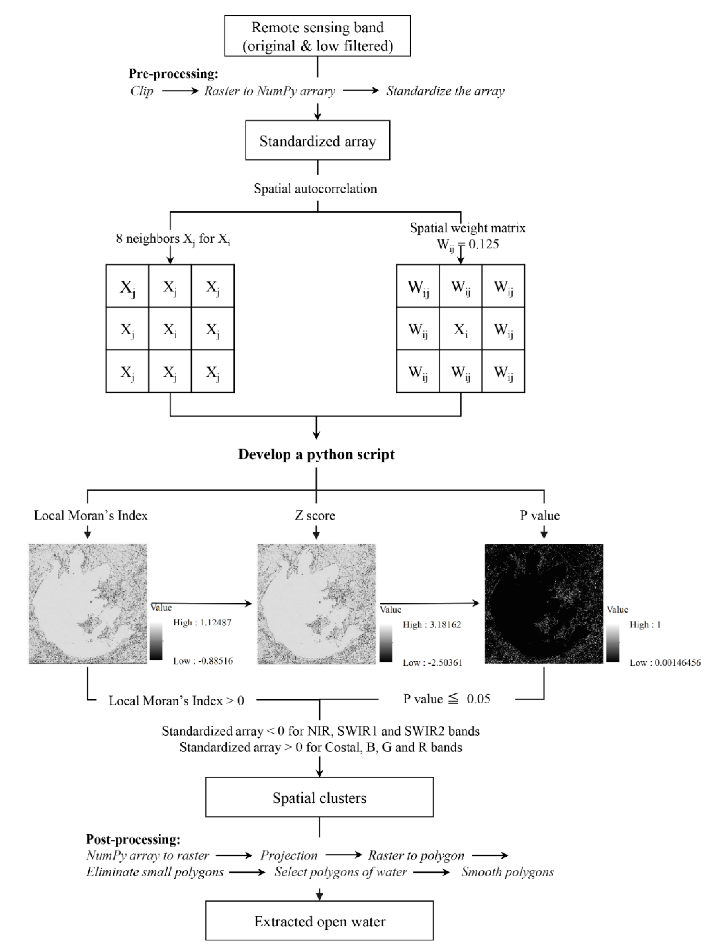
Processes for this study included pre-processing of Landsat single bands, analysis of spatial autocorrelation, and selecting significant low-value clusters. This final process meant identifying low–low clusters for the near-infrared band (NIR), first shortwave-infrared band (SWIR1), and second shortwave-infrared band (SWIR2), but high value clusters (high–high clusters) for coastal and three visible bands. Images were post-processed for low–low clusters on open surface water (Figure 2). Each single Landsat band, including the coastal band (i.e., for Landsat OLI image only), blue, green, red, NIR, SWIR1, and SWIR2 bands were tested separately for water extraction using the methods developed in this study. The specific steps are described here (see supplement materials for python script of all steps).

3.2.1. Pre-Processing of Landsat Single Bands

Pre-processing included clipping the imagery to the study area, converting rasters to a NumPy array, and standardizing the NumPy array (Equation (1)).

$$X=\frac{{\displaystyle \sum }{(R-\overline{R})}^2}{std\left(R\right)}$$

(1)

where $R$ is reflectance of each pixel for one Landsat single band, $\overline{R}$ is the mean, and $std\left(R\right)$ is the standard deviation of all pixels for one Landsat single band.

3.2.2. Spatial Autocorrelation for the Standardized NumPy Array

The surrounding eight pixels (X_j) were selected as spatial neighbors for the pixel X_i (Figure 2) to calculate spatial autocorrelation index $I_i$ (Equation (2) with equal spatial weight ($W_{ij})$ assigned to each of the eight neighbors = 1/8 = 0.125 (Figure 2). Equation (2) is based on the concept of Moran’s Index.

$$I_i=\frac{\left(n-1\right)X_i{{\displaystyle \sum }}_j{W}_{ij}{X}_j}{{{\displaystyle \sum }}_j{X}_j^2+X_i^2}$$

(2)

where $I_i$ is the spatial autocorrelation index that refers to the association (including statistical strength and direction of the association) between a given pixel and its spatial neighbors, $X_i$ is the standardized reflectance for one pixel of Landsat single band, $X_j$ is the spatial neighbor for $X_i$, $W_{ij}$ is the spatial weight, and $n$ is the total number of spatial neighbors (eight in this case).

The test statistic Z for significant test (standard normal distribution) for spatial autocorrelation $I_i$ is calculated by Equation (3) based on the concept of Moran’s Index.

$$\mathrm{Z}=\frac{I_i-E_I}{\sqrt{A-B-E_I^2}}$$

(3)

where $\mathrm{Z}$ is the test statistic from standard normal distribution, $I_i$ is the spatial autocorrelation index from Equation (2). $E_I$, $A,$ and $B$ are calculated from Equations (4), (5), and (6), respectively.

$$E_I=-\frac{1}{N-1}$$

(4)

where $N$ is the total number of pixels for the single Landsat band.

$$\mathrm{A}=\frac{8\times W_{ij}\times \left(N-b\right)}{N-1}$$

(5)

where $W_{ij}$ is the spatial weight for each neighbor, $N$ is the total number of pixels for the single Landsat band, and $b$ is calculated using Equation (7).

$$\mathrm{B}=\frac{27\times W_{ij}^2\times \left(2b-N\right)}{\left(N-1\right)\times \left(N-2\right)}$$

(6)

where $W_{ij}$ refers to the spatial weight for each neighbor, $N$ is the total number of pixels for the single Landsat band, and $b$ is calculated using Equation (7).

$$\mathrm{b}=\frac{{\displaystyle \sum }{\left(X-\overline{X}\right)}^4}{{\left({\displaystyle \sum }{\left(X-\overline{X}\right)}^2\right)}^2}$$

(7)

where $X$ is the standardized reflectance of each pixel for one Landsat single band, and $\overline{X}$ refers to the average value of the standardized array calculated by Equation (1).

The associated p-value from the test statistic Z in the significance test for spatial autocorrelation was calculated based on the python package: “scipy.stats”.

Low–low clusters (i.e., the first “low” means the value of $I_i$ is relatively low of the NumPy array, the second “low” means the value of its spatial neighbor is relatively low, and all low values are significantly, spatially clustered) for NIR, SWIR1, and SWIR2 bands, high–high clusters for coastal bands and three visible bands that refer to open surface water were selected from the standardized NumPy array based on three criteria: (1) $I_i$ > 0 (i.e., either high values or low values clustered together; (2) the value in the standardized array is less than zero (i.e., low values clusters are separate from high value clusters) for NIR, SWIR1, and SWIR2. For visible bands and the coastal band from Landsat OLI imagery, this criterion is slightly different (the standardized array larger than zero) because the reflectance of water in those bands is higher than other land cover types; and (3) p-value ≤ 0.05 (i.e., spatial autocorrelation index is statistically significant).

3.2.3. Post-Processing for Open Surface Water Extraction

The post-processing steps included converting the reassigned NumPy array to raster, defining the coordinate system for the converted raster, converting raster to polygon, eliminating small polygons (area less than 40,000 m²) that merge small polygons into the surrounding features (i.e., the minimum polygon area threshold were selected as 40,000 m² to reduce some effects of fish, crab, and shrimp farms which is near Taihu Lake for water extraction because the area of those farms are less than 40,000 m² in the study area), selecting polygons of open surface water, and smoothing polygons.

3.2.4. The Effects of Low Filter Image Process on Water Extraction

To mitigate noise from image quality, many studies introduce low filters to process images thereby improving feature accuracy and reducing illogical classification results from open water extraction [9,30]. The texture of open water is smoother than other land cover types from Landsat imagery, and the low filter process smooths open water features even more, which is effective to reduce the influence of image noise (i.e., salt and pepper effects from imagery). However, the low filter process might change the morphology and area of extracted open water from remotely sensed images. Therefore, a comparison was made of extracted open water area between low filtered and original images.

3.2.5. Time Series Analysis and Segmented Linear Regression for Climate and Survey Data

To capture an accurate annual precipitation trend, water level, and pondage data, seasonal effects were reduced using time series analysis (TSA) in Package “xts” (Extensible Time Series)) of R software (This software is from Bell Laboratories (Lucent Technologies) by John Chambers and colleagues, New Jersey, USA; It is initially written by Robert Gentleman and Ross Ihaka, Statistics Department of The University of Auckland, New Zealand). TSA separates regular seasonal variation and inter-annual trend from original temporal data (i.e., monthly data with 12 frequency per year). Then the results of annual trends were analyzed using the segmented linear relationship of Package “Segmented” in R software. The segmented linear relationship, which is also called broken-line relationship, is widely used in ecological research [56]. In this study, the segmented linear relationship was used to analyze thresholds for the inter-annual dynamics of precipitation, water level, and pondage data, as well as temporal change of the extracted Taihu area.

4. Results and Discussion

4.1. Open Water Extraction from Different Landsat Bands

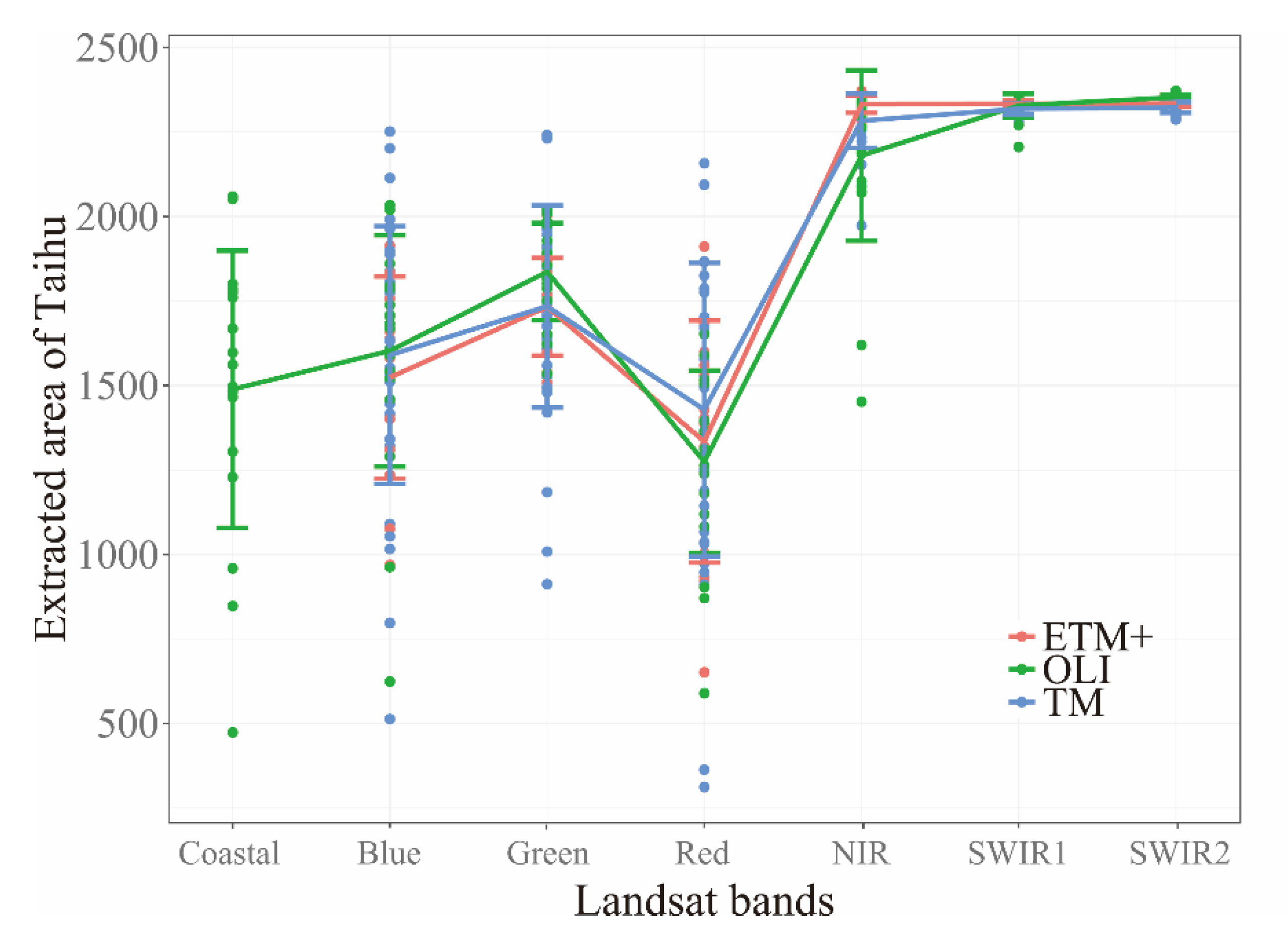
Among seven bands in the Landsat series, open water extraction from SWIR2 and SWIR1 is more stable than NIR, visible bands, and the coastal band from OLI imagery (Figure 3). NIR, SWIR1, and SWIR2 bands perform better for open surface water extraction (Figure 4, more example extractions in Supplementary A in the supplement materials), especially when the water was shallow and turbid. In 1984, when the water in Taihu Lake was clearer than previous years, most of the lake area was extracted from blue, green, and red bands, excluding the shallow area in eastern Taihu Lake and surrounding wetlands (Figure 4a–c). Since Taihu Lake became highly turbid after this, the visible Landsat bands were not suitable for open water extraction (Figure 4g–i). The extracted area from visible and coastal bands in Landsat OLI varied greatly under different water conditions (Figure 3). This is consistent with previous findings that NIR, SWIR1, and SWIR2 (i.e., TM band 4, 5, and 7) were typically used for open water extraction because water absorbed more completely in those bands than other land cover types [6].

The reflectance of clear water decreased with increasing wavelength in the optical domain (450–2500 nm) [5]. Therefore, reflectance of water in optical bands with long wavelength (NIR, SWIR1, and SWIR2) had lower values than other land cover types, which means water bodies were low value clusters in optical bands with long wavelengths. The methodology developed based on the concept of spatial autocorrelation is very suitable to detect low value clusters (i.e., low–low clusters or cold spots in spatial autocorrelation results). This method has greater potential to eliminate illogical results than other pixel-based classification methods because it emphasizes the autocorrelation of each pixel with its neighbors.

Gong’s (2017) results also show that spatial weights (i.e., an important parameter for local spatial autocorrelation models) would improve the temporal consistency of remote sensing classification [36]. However, water extraction using the methods from this study were influenced by other land cover types with low reflectance values (e.g., mountain and building shadows). Frazier and Page found TM band 5 (SWIR1) performed best for open water extraction, while TM bands 4 (NIR) and 7 (SWIR2) were less accurate [57]. Our results indicate that NIR was less accurate than SWIR1 and SWIR2 for open water extraction because it was influenced by “built-up noise” (Figure 4j). Therefore, extraction results from NIR overestimate actual open water area in some situations (Figure 3). The reason could be that “water-leaving radiance” contributed by NIR was significantly higher in the consistently turbid waters of Taihu Lake than that in clear water [58]. As with NIR, all three visible bands were affected by built-up noise during open water extraction (Figure 4g–i). Previous research indicates that normalized differences between green and SWIR1 that are equivalent to TM band 5, OLI band 6, or MODIS (Moderate Resolution Imaging Spectroradiometer) band 6 are best for open water extraction in various inundation extremes based on threshold algorithms [5,6], but are greatly influenced by dark surface noise in urban areas [27,28]. According to the results in this study, the noise of shadows in built-up areas comes from the green band instead of SWIR1 for open water extraction by the normalized difference between green and SWIR1.

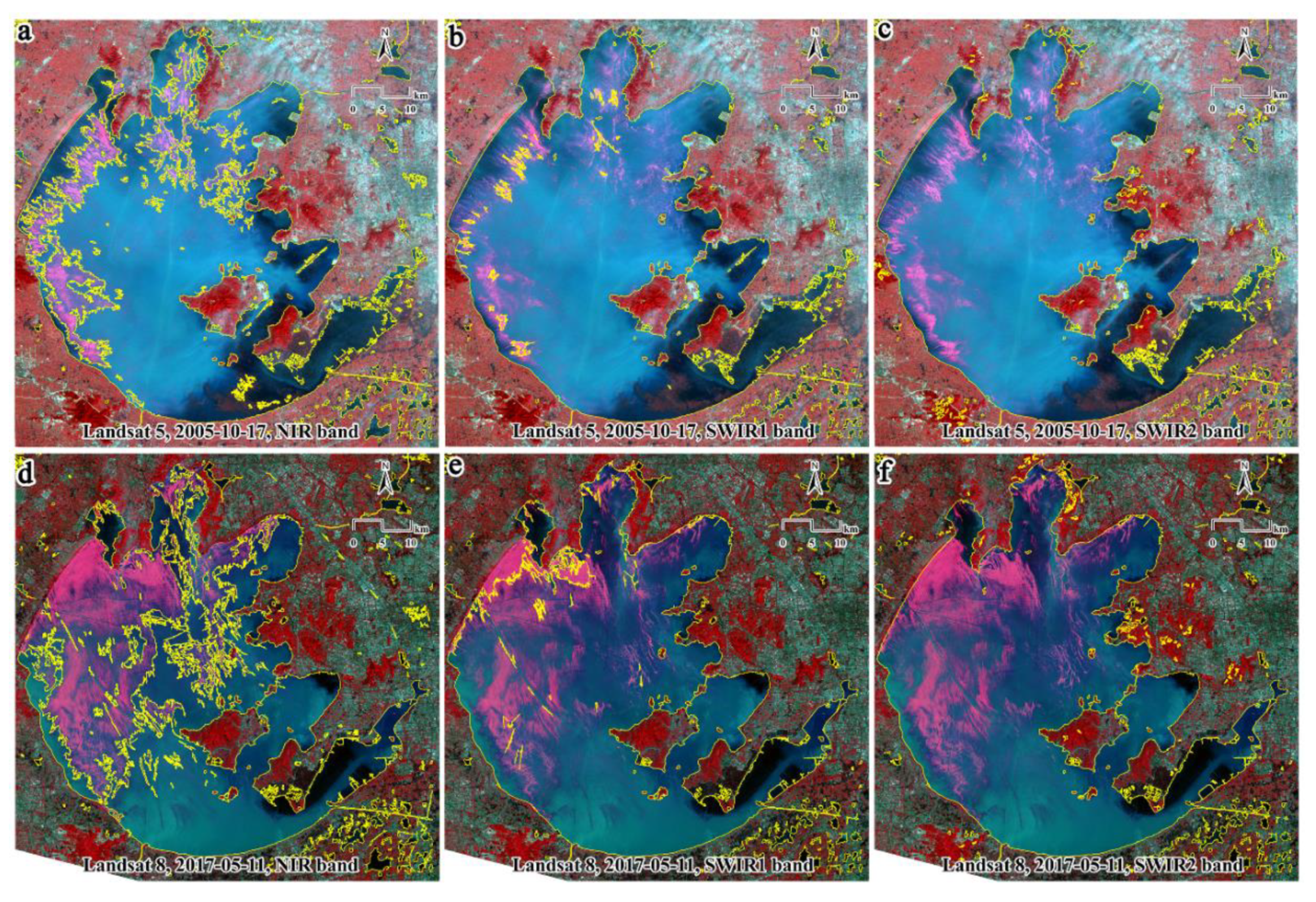
Water extraction from both SWIR1 and SWIR2 was slightly influenced by mountain shadows, and shadow effects on SWIR2 were stronger than SWIR1 (Figure 4k,l). Thus, our results indicate that SWIR1 is superior to SWIR2 and NIR for water extraction, which is consistent with Frazier and Page’s findings [57]. This is especially true when water is turbid and mountain shadows have similar spectral signals in Landsat imagery. However, SWIR2 has greater potential than SWIR1 and NIR to extract eutrophic open water with algal blooms (Figure 5). Even though the extraction area of Taihu Lake from SWIR2 was similar to that from SWIR1 (Figure 3), greater fluctuation of water extraction from SWIR1 than that from SWIR2 was due to the severe algal bloom in Taihu Lake (Figure 3 and Figure 5e). Part of the open water the algal bloom was excluded for open water extraction from SWIR1 (Figure 5b,e), while severe algal blooms and eutrophic water did not affect the water extraction process using SWIR2 based on the methodology in this study (Figure 5c,f). Using the NIR band, only open water uncovered by algal blooms was extracted, while water covered by algal blooms was excluded (Figure 5a,d). Therefore, NIR shows much less potential for open water extraction in Taihu Lake because the extracted water area from NIR varies among situations due to eutrophication and turbidity (Figure 3). Taking highly turbid water and severe algal blooms in Taihu Lake under consideration, SWIR2 is preferred for open water extraction. In this study, shadow effects for open water extraction from SIWR2 were controlled by a simple threshold using SWIR2 and the red band (i.e., $\left(SWIR2-Red\right)/\left(SWIR2+Red\right)<-0.2$: after exploring the spectral characteristics between water bodies and mountain shadows in the Landsat series, this threshold sufficiently reduced noise from mountain shadows).

The accuracy assessment was conducted based on the reference of Sentinel-2A images acquired in 2017-05-29, 2017-12-25, and 2019-11-15, paired with water extraction from Landsat OLI image acquired in 2017-05-27, 2017-12-21, and 2019-11-09 respectively. One hundred points were selected randomly in each image within the study area for accuracy assessment. The overall accuracy was 98% (more information about the accuracy assessment, error matrix, and the comparison between water extraction from Landsat OLI images and Sentinel-2A images are presented in Supplementary B of the supplement materials).

4.2. The Effects of Low Filter Image Processing on Water Extraction

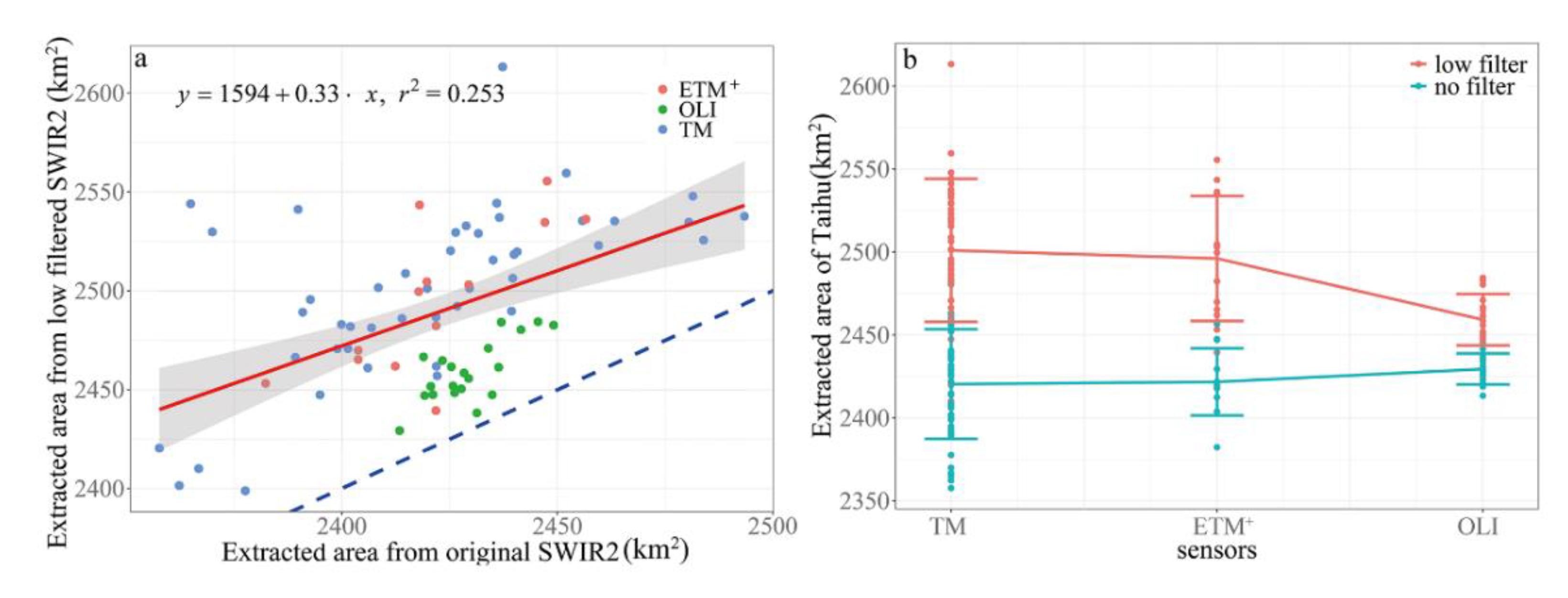
The area of extracted open water from low filtered SWIR2 imagery is overestimated compared to the original SWIR2 band from Landsat TM, ETM⁺, and OLI imagery (Figure 6a). The extraction results from low filtered and original SWIR2 are significantly different for either TM, ETM⁺, or OLI imagery (Figure 6b). Interestingly, the results from the low- and non-filtered OLI images were more similar to each other than the results of the Landsat TM and ETM⁺ (Figure 6). Olmanson’s research indicates that estimation result from Landsat OLI imagery is more homogeneous with less noise than that from Landsat 7 imagery [59]. This is because Landsat OLI (Landsat 8) imagery has a narrower multispectral band pattern than Landsat TM and ETM⁺. There are four TM images with extremely-high water areas identified in low filtered SWIR2 imagery not identified in the original imagery because those four images (acquisition dates: 1988-11-03, 1992-12-16, 1993-12-19, 1998-12-17) show visual salt and pepper noise (Figure 6a).

4.3. Temporal Trend of Extracted Area of Taihu Lake

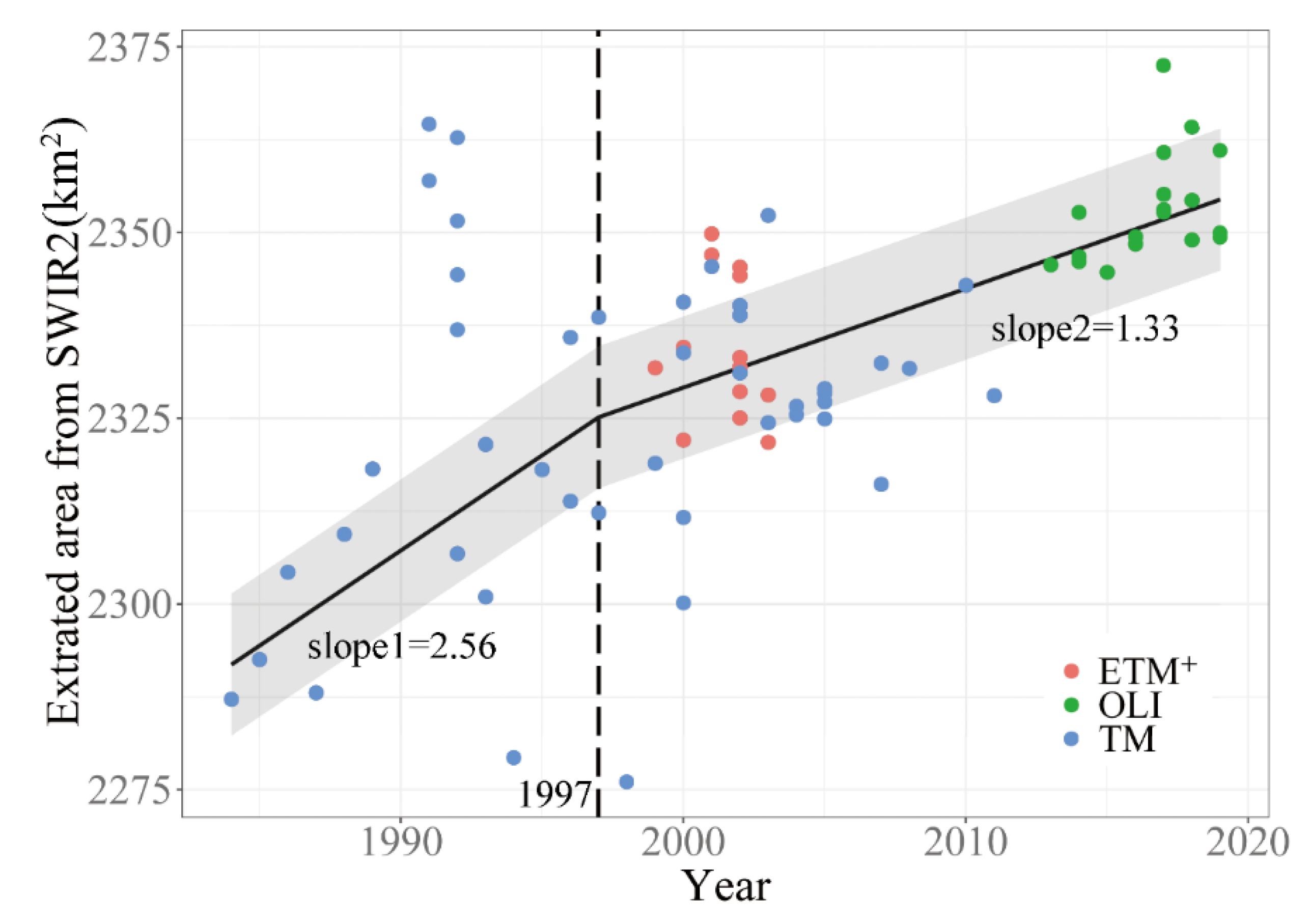
Finally, water extraction results based on the shadow-controlled SWIR2 band from 77 cloud free images with no image quality issues (i.e., salt and pepper) were selected to analyze the temporal trend of the dynamics in Taihu Lake (Figure 7; more extraction results are in Supplementary C of supplement materials). The area of Taihu Lake is relatively stable compared to other lakes with surrounding wetlands because Taihu Lake has cofferdams along most of its boundary. The temporal variation of the Taihu area was mainly caused by human activities including fish, crab and shrimp farms, wetland recovery, restoration from cultivation, and highway tunnel construction (Figure 8). Most dynamics were observed in Section 4, the south-east part of the lake (Figure 1), because of intensive anthropogenic disturbance (Figure 7). Since 1979, the surrounding wetlands in Section 4 that were once covered by reeds were gradually reclaimed as farms for fish, crab, or shrimp (Figure 7a–f). This increased the water area (Figure 8). Due to seasonal changes in water-covered farmlands that connect to the main lake, the extracted Taihu area had extremely high values in 1991 and 1992 (from images acquired in 1991-10-27, 1991-11-12, 1992-04-20, 1992-05-22, and 1992-06-07; Figure 7 and Figure 8). Since 1998, farmlands in the surrounding area of Section 4 were forbidden, so the abandoned farmlands were reclaimed by wetland grasses (Figure 7g) which led to a water area decrease from 1997 to 1998. However, the area of fish, crab, or shrimp farmlands gradually increased after 1998 at a slower rate compared to the period during 1979 to 1997 (Figure 8). Until 2008, policies forbidding farmland expansion were implemented again and the area of Taihu Lake dropped somewhat from 2008 to 2010 (Figure 7j and Figure 8). After 2010, a policy of lake restoration from cultivation was implemented and the area of Taihu Lake gradually increased (Figure 8). In addition, wetland recovery in the south-east part of Section 2 caused some variation in the lake area during 2004 to 2006 (Figure 7i), and the construction of highway tunnel also decreased the lake area slightly after 2018 (Figure 7l).

4.4. Inter-Annual Dynamics of Precipitation, Water Level and Pondage

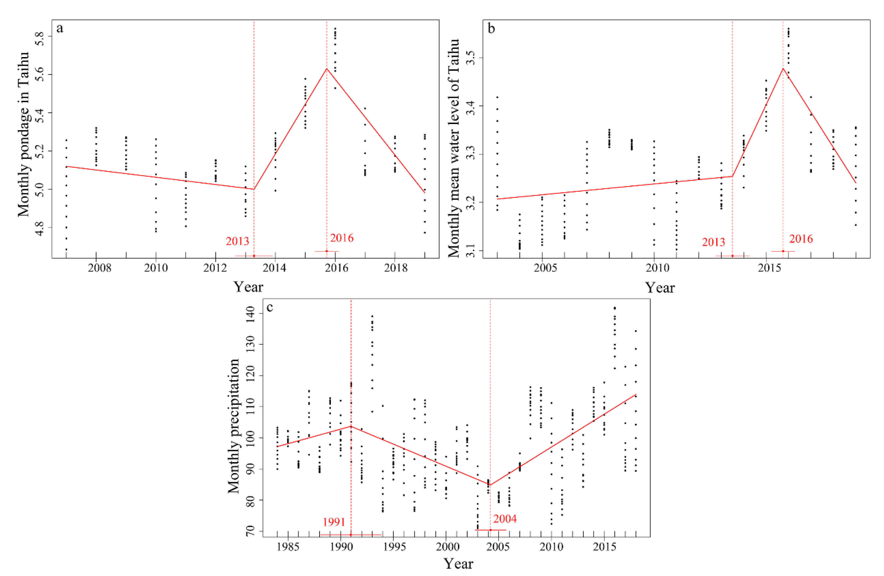
The temporal trend of pondage and water level was very consistent with the variation of inter-annual precipitation between 2007 and 2019 (Figure 9). However, temporal dynamics of Taihu Lake do not correspond to precipitation, water level, or pondage (Figure 8 and Figure 9). The area of Taihu Lake greatly increased from 1984 until 1997 (Figure 8), while precipitation was quite stable between 1984 to 1991 and decreased from 1991 to 2004 (Figure 9). Normally, the area of the shallow water region of the lake increases along with higher precipitation. Therefore, the increasing area of Taihu Lake between 1984 to 1997 was not caused by precipitation. The surrounding wetlands covered by reed in Section 4 of Taihu Lake (Figure 1) were gradually converted to parts of Taihu Lake (Figure 7). Those areas, unlike the original wetlands, were covered by water all year around, which were extracted as parts of Taihu Lake in the process of water extraction in this study.

4.5. Water Extraction in Different Sections of Taihu Lake

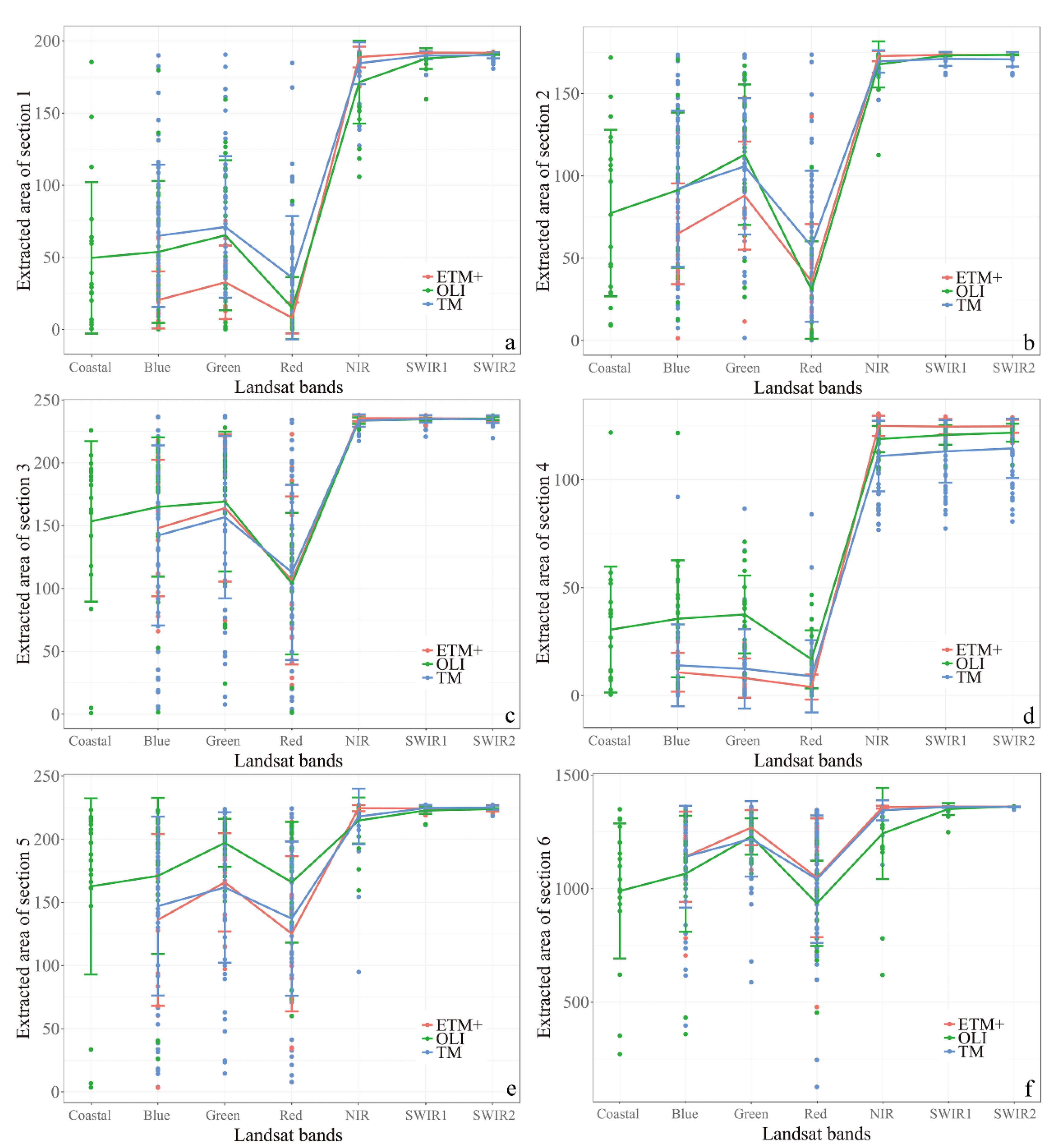
According to the extraction results from different Taihu Lake Sections based on all Landsat bands (Figure 10), NIR, SWIR1, and SWIR2 show significantly higher potential for water extraction than visible bands and the coastal band (from Landsat OLI only). For Sections 2, 3, and 4, the extraction area and its variation were consistent from NIR, SWIR1, and SWIR2 bands (Figure 10b–d). The extraction results from SWIR2 were clearly better than from SWIR1 as well as from NIR for Sections 1, 5, and 6 (Figure 10a,e,f). Sections 2, 3, and 4 are usually macrophyte-dominated regions with limited water surface covered by vegetation. Thus, submerged vegetation does not have much effect on water extraction from NIR or the SWIR1 band. However, Sections 1 and 6 are cyanobacteria-dominated, and Section 5 is largely dominated by floating-leaved vegetation, which challenges water extraction from the NIR band due to the vegetation covered water surface.

4.6. Error Sources of Automatic Open Water Extraction from Landsat Series

Some error sources, including cloud cover, image quality, polygon smoothing, and small polygon elimination, might lower the accuracy of automatic open water extraction from the Landsat series. Cloud shadows and thick clouds that cover water regions have a large impact on automatic open water extraction that use spatial autocorrelation (Supplementary D), while thin clouds, as well as thick clouds that are not above open water, do not influence on water extraction using NIR, SWIR1, or SWIR2 bands (Supplementary C: images acquired on 2004-10-14 and 2016-1-1). However, clouds have a strong influence on water extraction that use three visible bands because water has higher reflectance than other land cover types. This means that water bodies (as with cloud features) are high value clusters (i.e., hot spots in spatial autocorrelation analyses). The two post-processing steps for automatic water extraction, including polygon smoothing and small polygon elimination, were applied after the extracted raster was converted to a polygon. However, polygon smoothing might cause some variation (about 30 m shifts, similar to the spatial resolution of the Landsat series) for final extracted water boundaries and small polygon elimination (i.e., the area set for small polygons in the python script is 40,000 m²) might cause the loss of some small water bodies or wetlands. The advantage of the two steps is to reduce image quality effects on the classification results from traditional remote sensing classification methods, and to smooth the water bodies to bring them closer to the natural boundaries rather than the serrated boundaries caused by Landsat image spatial resolution.

5. Conclusions

The main purpose of this study was to develop a method based on the LISA concept to improve inland water extraction accuracy and temporal consistency in highly turbid and eutrophic water bodies with frequent anthropogenic disturbance. Using Landsat TM, ETM⁺, and OLI imagery, water extraction from the SWIR2 band using the developed methodology has great potential to extract inland water bodies automatically, even when the water is turbid and water surface is covered by algal blooms or floating vegetation. Our method with SWIR2 band greatly reduced the effects of vegetation surface cover compared to that of NIR, SWIR1, and visible bands. When the water surface was not covered by vegetation, NIR, SWIR1, and SWIR2 have consistent water extraction results; better than visible bands and the coastal band. Based on the methodology developed in this study, both SIWR1 and SWIR2 bands strongly eliminate noise from dark surfaces in urban areas compared to NIR and three visible bands.

Clouds and image quality (e.g., salt and pepper) have large impacts on automatic open water extraction based on the LISA concept. Low filter image processing is often applied to smooth the image for reducing salt and pepper effects in remotely sensed imagery, especially for water extraction due to the smooth texture of water bodies. However, comparing results between low filtered SWIR2 bands and original SWIR2 band, it appears that the low filter process overestimates extracted water areas. Our findings might enable global water extraction from multispectral imagery under various environmental conditions and image qualities.

References

- Bartsch, A.; Pathe, C.; Scipal, K.; Wagner, W. Detection of permanent open water surfaces in central Siberia with ENVISAT ASAR wide swath data with special emphasis on the estimation of methane fluxes from tundra wetlands. Hydrol. Res. 2008, 39, 89–100. [Google Scholar] [CrossRef]
- Zou, Z.; Xiao, X.; Dong, J.; Qin, Y.; Doughty, R.B.; Menarguez, M.A.; Zhang, G.; Wang, J. Divergent trends of open-surface water body area in the contiguous United States from 1984 to 2016. Proc. Natl. Acad. Sci. USA 2018, 115, 3810–3815. [Google Scholar] [CrossRef] [Green Version]
- Crasto, N.; Hopkinson, C.; Forbes, D.L.; Lesack, L.; Marsh, P.; Spooner, I.; van der Sanden, J.J. A LiDAR-based decision-tree classification of open water surfaces in an Arctic delta. Remote Sens. Environ. 2015, 164, 90–102. [Google Scholar] [CrossRef]
- Zhou, Y.; Dong, J.; Xiao, X.; Xiao, T.; Yang, Z.; Zhao, G.; Zou, Z.; Qin, Y. Open surface water mapping algorithms: A comparison of water-related spectral indices and sensors. Water 2017, 9, 256. [Google Scholar] [CrossRef]
- Colditz, R.R.; Troche Souza, C.; Vazquez, B.; Wickel, A.J.; Ressl, R. Analysis of optimal thresholds for identification of open water using MODIS-derived spectral indices for two coastal wetland systems in Mexico. Int. J. Appl. Earth Obs. Geoinf. 2018, 70, 13–24. [Google Scholar] [CrossRef]
- Liu, Z.; Yao, Z.; Wang, R. Assessing methods of identifying open water bodies using Landsat 8 OLI imagery. Environ. Earth Sci. 2016, 75. [Google Scholar] [CrossRef]
- Hardy, A.; Ettritch, G.; Cross, D.E.; Bunting, P.; Liywalii, F.; Sakala, J.; Silumesii, A.; Singini, D.; Smith, M.; Willis, T.; et al. Automatic detection of open and vegetated water bodies using sentinel 1 to map African malaria vector mosquito breeding habitats. Remote Sens. 2019, 11, 593. [Google Scholar] [CrossRef] [Green Version]
- Ticehurst, C.; Guerschman, J.P.; Chen, Y. The strengths and limitations in using the daily MODIS open water likelihood algorithm for identifying flood events. Remote Sens. 2014, 6, 11791–11809. [Google Scholar] [CrossRef] [Green Version]
- Reiter, M.E.; Elliott, N.; Veloz, S.; Jongsomjit, D.; Hickey, C.M.; Merrifield, M.; Reynolds, M.D. Spatio-temporal patterns of open surface water in the central valley of California 2000–2011: Drought, land cover, and waterbirds. J. Am. Water Resour. Assoc. 2015, 51, 1722–1738. [Google Scholar] [CrossRef] [Green Version]
- Santoro, M.; Wegmueller, U.; Lamarche, C.; Bontemps, S.; Defoumy, P.; Arino, O. Strengths and weaknesses of multi-year Envisat ASAR backscatter measurements to map permanent open water bodies at global scale. Remote Sens. Environ. 2015, 171, 185–201. [Google Scholar] [CrossRef]
- Santoro, M.; Wegmueller, U.; Wiesmann, A.; Lamarche, C.; Bontemps, S.; Defourny, P.; Arino, O. Assessing fnvisat ASAR and sentinel-1 multi-temporal observations to map open water bodies. In Proceedings of the 2015 IEEE 5th Asia-Pacific Conference on Synthetic Aperture Radar, Singapore, 1–4 September 2015; pp. 614–619. [Google Scholar]
- Cutler, P.J.; Schwartzkopf, W.C.; Koehler, F.W. Robust automated thresholding of SAR imagery for open-water detection. In Proceedings of the 2015 IEEE International Radar Conference, Arlington, VA, USA, 11–15 May 2015; pp. 310–315. [Google Scholar]
- Santoro, M.; Wegmueller, U. Multi-temporal synthetic aperture radar metrics applied to map open water bodies. IEEE J. Sel. Top. Appl. Earth Obs. Remote Sens. 2014, 7, 3225–3238. [Google Scholar] [CrossRef]
- Bioresita, F.; Puissant, A.; Stumpf, A.; Malet, J.-P. A method for automatic and rapid mapping of water surfaces from sentinel-1 imagery. Remote Sens. 2018, 10, 217. [Google Scholar] [CrossRef] [Green Version]
- van Leeuwen, B.; Tobak, Z.; Kovacs, F. Sentinel-1 and-2 based near real time inland excess water mapping for optimizedwater management. Sustainability 2020, 12, 2854. [Google Scholar] [CrossRef] [Green Version]
- Geldsetzer, T.; Yackel, J.J. Sea ice type and open water discrimination using dual co-polarized C-band SAR. Can. J. Remote Sens. 2009, 35, 73–84. [Google Scholar] [CrossRef]
- Karvonen, J.; Simila, M.; Makynen, M. Open water detection from Baltic Sea ice Radarsat-1 SAR imagery. IEEE Geosci. Remote Sens. Lett. 2005, 2, 275–279. [Google Scholar] [CrossRef]
- Komarov, A.S.; Buehner, M. Automated detection of ice and open water from dual-polarization RADARSAT-2 images for data assimilation. IEEE Trans. Geosci. Remote Sens. 2017, 55, 5755–5769. [Google Scholar] [CrossRef]
- Komarov, A.S.; Buehner, M. Adaptive probability thresholding in automated ice and open water detection from RADARSAT-2 images. IEEE Geosci. Remote Sens. Lett. 2018, 15, 552–556. [Google Scholar] [CrossRef]
- Schmitt, M. Potential of large-scale inland water body mapping from Sentinel-1/2 data on the example of Bavaria′s lakes and rivers. PFG J. Photogramm. Remote Sens. Geoinf. Sci. 2020. [Google Scholar] [CrossRef]
- Ovakoglou, G.; Alexandridis, T.K.; Crisman, T.L.; Skoulikaris, C.; Vergos, G.S. Use of MODIS satellite images for detailed lake morphometry: Application to basins with large water level fluctuations. Int. J. Appl. Earth Obs. Geoinf. 2016, 51, 37–46. [Google Scholar] [CrossRef]
- Goffi, A.; Stroppiana, D.; Brivio, P.A.; Bordogna, G.; Boschetti, M. Towards an automated approach to map flooded areas from Sentinel-2 MSI data and soft integration of water spectral features. Int. J. Appl. Earth Obs. Geoinf. 2020, 84. [Google Scholar] [CrossRef]
- Kutser, T.; Paavel, B.; Kaljurand, K.; Ligi, M.; Randla, M. Mapping shallow waters of the Baltic sea with Sentinel-2 imagery. In Proceedings of the 2018 IEEE/OES Baltic International Symposium, Klaipèda, Lithuania, 12–15 June 2018. [Google Scholar]
- Arvor, D.; Daher, F.R.G.; Briand, D.; Dufour, S.; Rollet, A.-J.; Simoes, M.; Ferraz, R.P.D. Monitoring thirty years of small water reservoirs proliferation in the southern Brazilian Amazon with Landsat time series. ISPRS J. Photogramm. Remote Sens. 2018, 145, 225–237. [Google Scholar] [CrossRef]
- Pekel, J.-F.; Cottam, A.; Gorelick, N.; Belward, A.S. High-resolution mapping of global surface water and its long-term changes. Nature 2016, 540, 418–422. [Google Scholar] [CrossRef] [PubMed]
- Sekertekin, A. A survey on global thresholding methods for mapping open water body using sentinel-2 satellite imagery and normalized difference water index. Arch. Comput. Methods Eng. 2020. [Google Scholar] [CrossRef]
- Xu, H. Modification of normalised difference water index (NDWI) to enhance open water features in remotely sensed imagery. Int. J. Remote Sens. 2006, 27, 3025–3033. [Google Scholar] [CrossRef]
- Feyisa, G.L.; Meilby, H.; Fensholt, R.; Proud, S.R. Automated water extraction index: A new technique for surface water mapping using Landsat imagery. Remote Sens. Environ. 2014, 140, 23–35. [Google Scholar] [CrossRef]
- Yue, H.; Liu, Y. Method for delineating open water bodies based on the deeply clear waterbody delineation index. J. Appl. Remote Sens. 2019, 13. [Google Scholar] [CrossRef]
- Lira, J. Segmentation and morphology of open water bodies from multispectral images. Int. J. Remote Sens. 2006, 27, 4015–4038. [Google Scholar] [CrossRef]
- Liu, S.; Su, H.; Cao, G.; Wang, S.; Guan, Q. Learning from data: A post classification method for annual land cover analysis in urban areas. ISPRS J. Photogramm. Remote Sens. 2019, 154, 202–215. [Google Scholar] [CrossRef]
- Chemin, Y.; Rabbani, U. A new methodology for virtual water level gauges. Int. J. Geoinf. 2016, 12, 15–25. [Google Scholar]
- Wang, L.; Shi, C.; Diao, C.; Ji, W.; Yin, D. A survey of methods incorporating spatial information in image classification and spectral unmixing. Int. J. Remote Sens. 2016, 37, 3870–3910. [Google Scholar] [CrossRef]
- Holden, Z.A.; Evans, J.S. Using fuzzy C-means and local autocorrelation to cluster satellite-inferred burn severity classes. Int. J. Wildland Fire 2010, 19, 853–860. [Google Scholar] [CrossRef]
- Kowe, P.; Mutanga, O.; Odindi, J.; Dube, T. Exploring the spatial patterns of vegetation fragmentation using local spatial autocorrelation indices. J. Appl. Remote Sens. 2019, 13. [Google Scholar] [CrossRef]
- Gong, W.; Fang, S.; Yang, G.; Ge, M. Using a hidden markov model for improving the spatial-temporal consistency of time series land cover classification. ISPRS Int. J. Geo-inf. 2017, 6, 292. [Google Scholar] [CrossRef] [Green Version]
- Luo, J.; Pu, R.; Duan, H.; Ma, R.; Mao, Z.; Zeng, Y.; Huang, L.; Xiao, Q. Evaluating the influences of harvesting activity and eutrophication on loss of aquatic vegetations in Taihu Lake, China. Int. J. Appl. Earth Obs. Geoinf. 2020, 87. [Google Scholar] [CrossRef]
- Sun, D.Y.; Li, Y.M.; Wang, Q.; Lu, H.; Le, C.F.; Huang, C.C.; Gong, S.Q. A neural-network model to retrieve CDOM absorption from in situ measured hyperspectral data in an optically complex lake: Lake Taihu case study. Int. J. Remote Sens. 2011, 32, 4005–4022. [Google Scholar] [CrossRef]
- Sun, D.; Li, Y.; Wang, Q.; Le, C.; Huang, C.; Wang, L. Parameterization of water component absorption in an inland eutrophic lake and its seasonal variability: A case study in Lake Taihu. Int. J. Remote Sens. 2009, 30, 3549–3571. [Google Scholar] [CrossRef]
- Ma, R.; Duan, H.; Gu, X.; Zhang, S. Detecting aquatic vegetation changes in Taihu Lake, China using multi-temporal satellite imagery. Sensors 2008, 8, 3988–4005. [Google Scholar] [CrossRef] [Green Version]
- Huang, C.; Jiang, Q.; Yao, L.; Li, Y.; Yang, H.; Huang, T.; Zhang, M. Spatiotemporal variation in particulate organic carbon based on long-term MODIS observations in Taihu Lake, China. Remote Sens. 2017, 9, 624. [Google Scholar] [CrossRef] [Green Version]
- Wang, S.; Gao, Y.; Li, Q.; Gao, J.; Zhai, S.; Zhou, Y.; Cheng, Y. Long-term and inter-monthly dynamics of aquatic vegetation and its relation with environmental factors in Taihu Lake, China. Sci. Total Environ. 2019, 651, 367–380. [Google Scholar] [CrossRef]
- Huang, C.; Yang, H.; Zhu, A.X.; Zhang, M.; Lu, H.; Huang, T.; Zou, J.; Li, Y. Evaluation of the Geostationary Ocean Color Imager (GOCI) to monitor the dynamic characteristics of suspension sediment in Taihu Lake. Int. J. Remote Sens. 2015, 36, 3859–3874. [Google Scholar] [CrossRef]
- Chen, J.; Quan, W. Using Landsat/TM imagery to estimate nitrogen and phosphorus concentration in Taihu Lake, China. IEEE J. Sel. Top. Appl. Earth Obs. Remote Sens. 2012, 5, 273–280. [Google Scholar] [CrossRef]
- Jia, T.; Zhang, X.; Dong, R. Long-term spatial and temporal monitoring of cyanobacteria blooms using MODIS on google earth engine: A case study in Taihu Lake. Remote Sens. 2019, 11, 2269. [Google Scholar] [CrossRef] [Green Version]
- Zhang, Y.; Shi, K.; Zhou, Y.; Liu, X.; Qin, B. Monitoring the river plume induced by heavy rainfall events in large, shallow, Lake Taihu using MODIS 250 m imagery. Remote Sens. Environ. 2016, 173, 109–121. [Google Scholar] [CrossRef]
- Qi, L.; Hu, C.; Duan, H.; Barnes, B.B.; Ma, R. An EOF-based algorithm to estimate chlorophyll a concentrations in Taihu Lake from MODIS land-band measurements: Implications for near real-time applications and forecasting models. Remote Sens. 2014, 6, 10694–10715. [Google Scholar] [CrossRef] [Green Version]
- Le, C.; Li, Y.; Zha, Y.; Sun, D.; Huang, C.; Lu, H. A four-band semi-analytical model for estimating chlorophyll a in highly turbid lakes: The case of Taihu Lake, China. Remote Sens. Environ. 2009, 113, 1175–1182. [Google Scholar] [CrossRef]
- Cheng, C.; Wei, Y.; Lv, G.; Yuan, Z. Remote estimation of chlorophyll-a concentration in turbid water using a spectral index: A case study in Taihu Lake, China. J. Appl. Remote Sens. 2013, 7. [Google Scholar] [CrossRef] [Green Version]
- Shi, W.; Zhang, Y.; Wang, M. Deriving total suspended matter concentration from the near-infrared-based inherent optical properties over turbid waters: A case study in Lake Taihu. Remote Sens. 2018, 10, 333. [Google Scholar] [CrossRef] [Green Version]
- Li, J.; Hu, C.; Shen, Q.; Barnes, B.B.; Murch, B.; Feng, L.; Zhang, M.; Zhang, B. Recovering low quality MODIS-Terra data over highly turbid waters through noise reduction and regional vicarious calibration adjustment: A case study in Taihu Lake. Remote Sens. Environ. 2017, 197, 72–84. [Google Scholar] [CrossRef]
- Zhang, F.; Li, J.; Shen, Q.; Zhang, B.; Tian, L.; Ye, H.; Wang, S.; Lu, Z. A soft-classification-based chlorophyll-a estimation method using MERIS data in the highly turbid and eutrophic Taihu Lake. Int. J. Appl. Earth Obs. Geoinf. 2019, 74, 138–149. [Google Scholar] [CrossRef]
- Deng, Y.; Zhang, Y.; Li, D.; Shi, K.; Zhang, Y. Temporal and spatial dynamics of phytoplankton primary production in Lake Taihu derived from MODIS data. Remote Sens. 2017, 9, 195. [Google Scholar] [CrossRef]
- Luo, J.; Ma, R.; Duan, H.; Hu, W.; Zhu, J.; Huang, W.; Lin, C. A new method for modifying thresholds in the classification of tree models for mapping aquatic vegetation in Taihu Lake with satellite images. Remote Sens. 2014, 6, 7442–7462. [Google Scholar] [CrossRef] [Green Version]
- Liang, Q.; Zhang, Y.; Ma, R.; Loiselle, S.; Li, J.; Hu, M. A MODIS-based novel method to distinguish surface cyanobacterial scums and aquatic macrophytes in Lake Taihu. Remote Sens. 2017, 9, 133. [Google Scholar] [CrossRef] [Green Version]
- Xu, D.D.; Guo, X.L.; Li, Z.Q.; Yang, X.H.; Yin, H. Measuring the dead component of mixed grassland with Landsat imagery. Remote Sens. Environ. 2014, 142, 33–43. [Google Scholar] [CrossRef]
- Frazier, P.S.; Page, K.J. Water body detection and delineation with Landsat TM data. Photogramm. Eng. Remote Sens. 2000, 66, 1461–1467. [Google Scholar]
- Wang, M.; Shi, W.; Tang, J. Water property monitoring and assessment for China’s inland Lake Taihu from MODIS-Aqua measurements. Remote Sens. Environ. 2011, 115, 841–854. [Google Scholar] [CrossRef]
- Olmanson, L.G.; Brezonik, P.L.; Finlay, J.C.; Bauer, M.E. Comparison of Landsat 8 and Landsat 7 for regional measurements of CDOM and water clarity in lakes. Remote Sens. Environ. 2016, 185, 119–128. [Google Scholar] [CrossRef]
Figure 1.
The Taihu Lake study area. The background image is a Landsat TM (Thematic Mapper) scene acquired on 1999-02-03 with standard false color composition (near-infrared band in red, red band in green, and green band in blue).
Figure 2.
Methodology flowchart. B = blue band; G = Green band; R = Red band; NIR = Near-infrared band; SWIR1 = first shortwave infrared band; SWIR2 = second shortwave infrared band; Spatial clusters = low–low clusters (i.e., low value pixels significantly cluster together spatially) or high–high clusters (i.e., high value pixels significantly cluster together spatially).
Figure 3.
The area of extracted Taihu Lake across Landsat bands. TM = Thematic Mapper; ETM+ = Enhanced Thematic Mapper; OLI = Operational Land Imager.
Figure 4.
Sample water extraction results of Landsat TM imagery (the yellow line is the extracted water boundary, and the background image is with standard false color composition). Water extraction results from blue (a), green (b), red (c), near infrared (d), first shortwave infrared (e), and second shortwave infrared bands (f) of Landsat TM acquired in 1984-08-04. Water extraction results from blue (g), green (h), red (i), near infrared (j), first shortwave infrared (k), and second shortwave infrared (l) bands of Landsat TM acquired in 1997-05-04.
Figure 5.
Sample water extraction results for water bloom effected water bodies (the yellow line is the extracted water boundary, and the background image is with standard false color composition). Water extraction results from near infrared (a), first shortwave infrared (b), and second shortwave infrared bands (c) of Landsat TM (Thematic Mapper) acquired in 2005-10-17. Extraction results from near infrared (d), first shortwave infrared (e) and second shortwave infrared bands (f) of Landsat OLI (Operational Land Imager) acquired in 2017-05-11.
Figure 6.
Comparison of extracted area by low and non-filtered imagery among three sensors. (a): comparison between the area of water extraction from low-filtered SWIR2 (second shortwave-infrared band) and original SWIR2. (b): error bar graph for extracted water area of low-filtered and original SWIR2 among three different sensors (TM = Thematic Mapper; ETM+ = Enhanced Thematic Mapper; OLI = Operational Land Imager).
Figure 7.
Water extraction for Taihu Lake during 1984–2019 using Landsat series images (the yellow line is the extracted water boundary, and the background image uses standard false color composition). Water extraction results from second shortwave-infrared band (SWIR2) of Landsat TM (Thematic Mapper) acquired in 1985-01-11 (a), 1989-10-21 (b), 1991-11-12 (c), 1992-07-25(d), 1994-06-29 (e), 1995-02-24 (f), 1998-08-11 (g), 2000-12-06 (h), 2005-04-08 (i), 2010-05-24 (j), and of Landsat OLI (Operational Land Imager) acquired in 2015-10-13 (k) and 2019-11-09 (l).
Figure 8.
Temporal trend of extracted area in Taihu Lake from 1984 to 2019 (TM = Thematic Mapper; ETM+ = Enhanced Thematic Mapper; OLI = Operational Land Imager).