A New Method of De-Aliasing Large-Scale High-Frequency Barotropic Signals in the Mediterranean Sea


1
CAS Key Laboratory of Ocean Circulation and Waves, Institute of Oceanology, Chinese Academy of Sciences, Qingdao 266071, China
2
University of Chinese Academy of Sciences, Beijing 100049, China
3
Center for Ocean Mega-Science, Chinese Academy of Sciences, Qingdao 266071, China
4
Laboratoire d’Oceanographie Physique et Spatiale, Institut Français de Recherche pour l’Exploitation de la Mer (IFREMER), 29280 Plouzané, France
*
Author to whom correspondence should be addressed.
Remote Sens. 2020, 12(13), 2157; https://doi.org/10.3390/rs12132157
Submission received: 25 May 2020
/
Revised: 1 July 2020
/
Accepted: 2 July 2020
/
Published: 6 July 2020
(This article belongs to the Special Issue Advances in Ocean Remote Sensing through Data and Algorithm Fusion)
Abstract
:With the development of satellite observation technology, higher resolution and shorter return cycle have also placed higher demands on satellite data processing. The non-tide high-frequency barotropic oscillation in the marginal sea produces large aliasing errors in satellite altimeter observations. In previous studies, the satellite altimeter aliasing correction generally relied on a few bottom pressure data or the model data. Here, we employed the high-frequency tide gauge data to extract the altimeter non-tide aliasing correction in the west Mediterranean Sea. The spatial average method and EOF analysis method were adopted to track the high-frequency oscillation signals from 15 tide gauge records (TGs), and then were used to correct the aliasing errors in the Jason-1 and Envisat observations. The results showed that the EOF analysis method is better than the spatial average method in the altimeter data correction. After EOF correction, 90% of correlation (COR) between TG and sea level of Jason-1 has increased ~5%, and ~3% increase for the Envisat sea level; for the spatial average correction method, only ~70% of Jason-1 and Envisat data at the TGs location has about 2% increase in correlation. The EOF correction reduced the average percentage of error variance (PEL) by ~30%, while the spatial average correction increased the average percentage of PEL by ~20%. After correction by the EOF method, the altimeter observations are more consistent with the distribution of strong currents and eddies in the west Mediterranean Sea. The results prove that the proposed EOF method is more effective and accurate for the non-tide aliasing correction.

1. Introduction
Satellite altimeter can only monitor phenomena with periods longer than twice of the satellite period (i.e., Nyquist frequency) [1]. The gridded datasets of satellite altimeter are merged from the along-track data. In order to study ocean events at a different time and space scales, efforts are made to improve the accuracy of the altimeter along-track data [2,3] and the mapping method [4]. However, due to the limitation of the sampling frequency, the existence of non-tide high-frequency barotropic motions in the ocean can lead to indistinguishable signal errors in satellite altimeter observations, called aliasing. These high-frequency non-tide signals with the period from 2.5 days to twice the satellite repeat cycle (2) have an irregular nature in terms of scale, intensity, and geographical distribution. Quinn and Ponte [5] illustrated the problem in the modeling of non-tidal sea level variations by comparing two different baroclinic ocean models with pressure gauges. They found that there are very large differences in the high-frequency bands, and the large high-frequency barotropic signals from pressure records may cause significant aliased errors in monthly altimetry sea level observations. In the semi-enclosed sea, this aliasing errors in altimetry observation may typically be double that of open oceans due to the influence of their boundaries and lower accuracy in high-frequency signal corrections [6,7,8]. Xu et al. [8] and Li and Xu [9] demonstrated that the high-frequency barotropic motions in the Japan Sea is uniform in the basin, named common mode. It has caused aliasing errors in altimeter observations and may increase as the data merge. Moreover, they can affect the observation of mesoscale eddies and long-period signal analysis.
Previous studies generally relied on the high time resolution in situ data or model data to extract the high-frequency motions for the aliasing error correction. The high time resolution BP data and the tide gauges (TGs) data were used to extract the basin-wide high-frequency motion through the spatial average method [8,9,10]. This method is based on the assumption that local high-frequency signals that can be offset by averaging. It is only suitable for absolutely uniform high-frequency motion in space, because the large inconsistency of local high-frequency signals in space may corrupt the altimeter measurements, rather than correction. Li and Xu [9] shown that, compared with TGs data, the bottom pressure (BP) measurements located in the middle of the Japan Sea can obtain better correction results, while TGs may not be consistent at the edge of the basin. In this study, we propose to use the Empirical Orthogonal Function (EOF) analysis method to identify and quantify the dominating part of the spatial and temporal variability for the aliasing error correction [11]. The EOF has been widely used in climatology, meteorology, and oceanography [11,12,13]. Fukumori et al. [14] investigated the high-frequency motion in the Mediterranean Sea by the EOF method from the altimeter data and model data. They found that high-frequency (less than 70 day) basin-wide barotropic oscillations account for ~50% of altimeter sea level root mean square (RMS) amplitude [8]. The altimeter cannot reveal ocean events whose timescale is less than two times of the altimetry cycle period (), such as the threshold for the Jason-1 and Envisat is 20 and 70 days (Nyquist period), respectively. Over the past decade, satellite observations or models have been used to study the basin-scale signals in the Mediterranean Sea [6,14,15,16]. However, the influence of basin-scale aliasing in gridded products from multi-altimeter missions is still unclear.
In this study, we evaluate the effect of two types of methods in the altimetry aliasing error correction in the west Mediterranean Sea (Figure 1). Jason-1 and Envisat observations are used in this study. Jason-1 and Envisat have 10 and 35 days of repeating cycles, respectively, and repeating cycles of most altimeter satellites are somewhere in between. This assessment focuses on the de-aliasing impact of the altimetry gridded products using TGs records (Figure 2). Compared with the rare BP data records, the TGs data has more longer records and easier to obtain, which has a large potential for the study of the aliasing error corrected by the altimeter. In addition, the dynamics mechanism of the nonlinear aliasing will be these non-tide high-frequency signals are also discussed.
2. Materials and Methods
2.1. TG Data and Pre-Processing
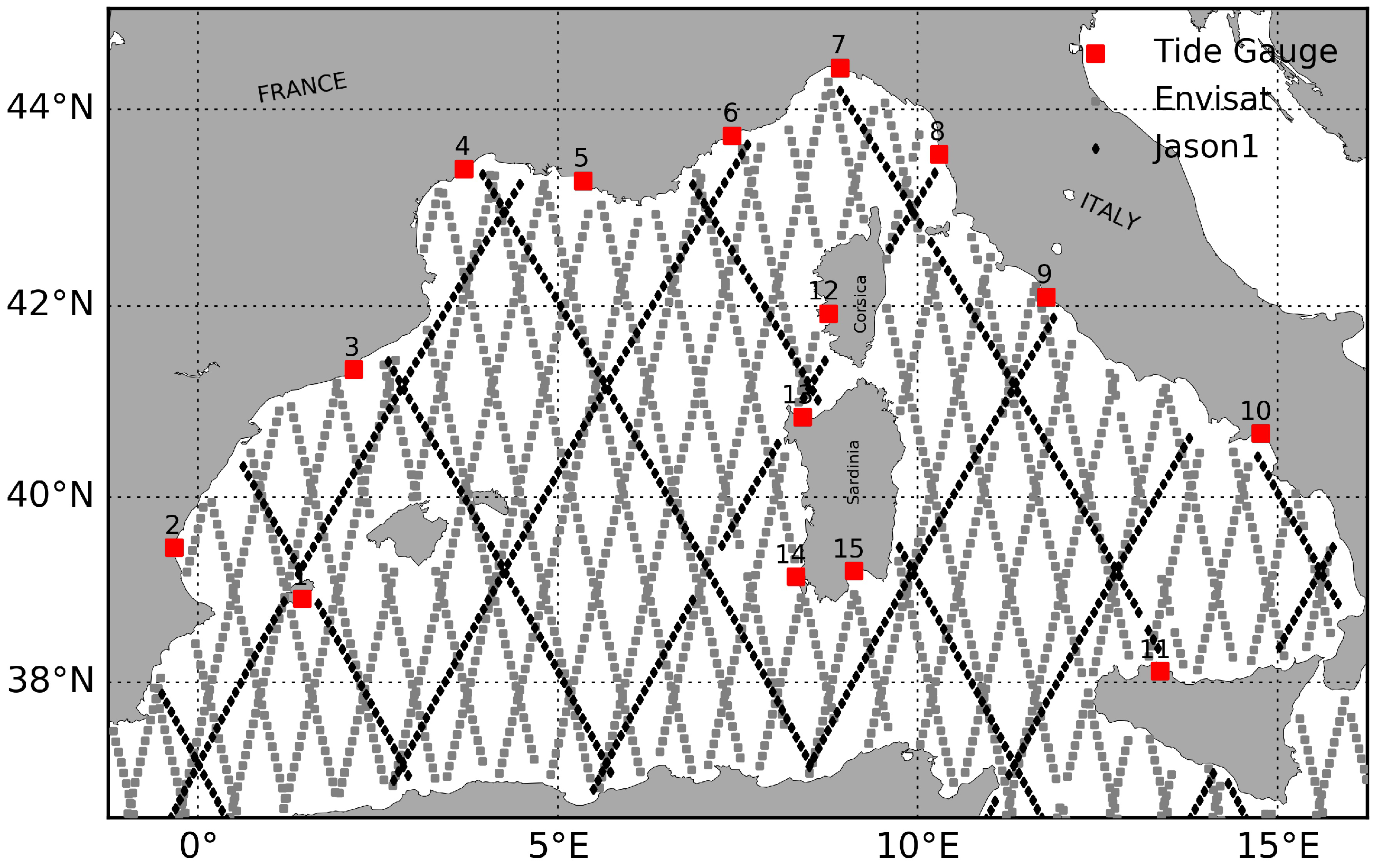
The TG sea level records of the west Mediterranean Sea were obtained from the GESLA-2 (Global Extreme Sea Level Analysis, version 2) dataset [18]. This dataset collected 1355 records and 39,151 station-years of tide gauge data from 30 source agencies on a global scale with hourly or higher (e.g., 6- or 15-min) time resolution, and it was also distributed by the British Oceanographic Data Centre (BODC). The dataset with higher-frequency are not necessary better, primarily because the faster sampling has a challenge in the data recording and verification. In the Mediterranean Sea, there are 57 tide gauge stations of the GESLA-2 covering the period from 1992 to 2012 (respond to the satellite). Only about 30% of the stations have a complete time series. In order to avoid the error caused by the multiple time resolutions and obtain TG data more suitable to aliasing error correction, the higher time resolution TGs data were sampled to 1 hour resolution by one-dimensional linear interpolation of two adjacent records. We selected TG data according to following criteria; first, the good TGs data accounted for more than 80% of the total records for the entire study period (Record Pct.); second, the selected TG stations should be evenly distributed throughout the research area and far away from straits (like the Gibraltar Strait) to avoid the influence of strong local signals or other signals. We finally selected 15 TG stations, which accounted for at least 80% of the complete time series from 2003 to 2006 and evenly distributed in the west Mediterranean Sea (wMED). Figure 2 shows the geographic location of the selected tide gauge stations (red squares) over the basin. More detailed information of these tide gauge stations is listed in Table 1.
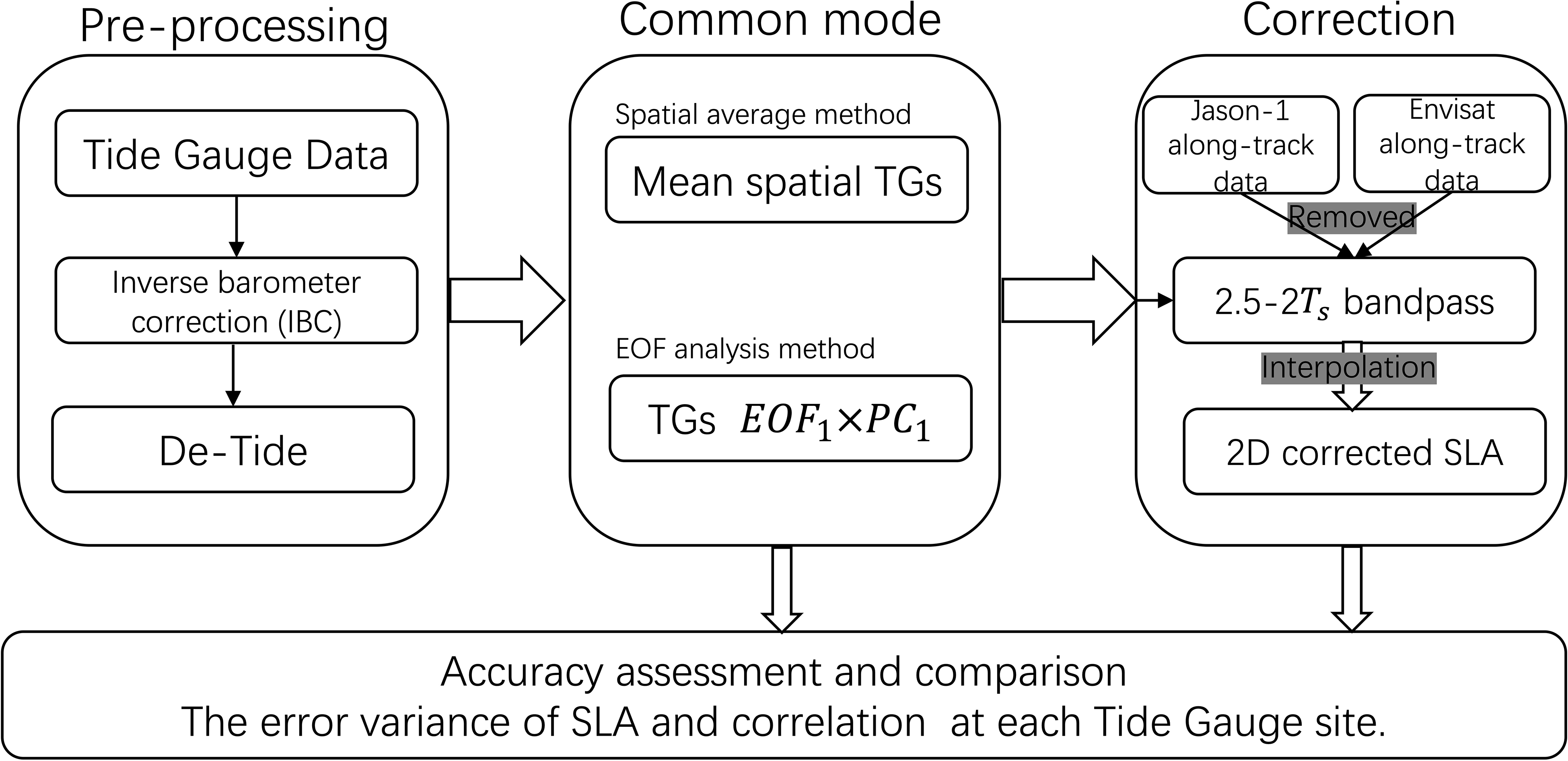
As follow the procedure of Xu et al. [8], two known high-frequency signals were removed from the TG data before the common mode was extracted. One is the high frequency sea level variability caused by atmospheric pressure, i.e., inverse barometer correction (IBC). The other is the tidal oscillations, because aliasing error associated with the ocean tides could be a major source of systematic error in altimeter sea-level measurements [1,19,20,21]. We used the sea level pressure field data from the Centre for Medium-Range Weather Forecasts (ECMWF) Reanalysis dataset (ERA-Interim) for IBC. The pressure data has a spatial resolution of and 6 h time resolution [22]. They were spatial-temporally interpolated to obtain 10 m atmospheric pressure data () time series corresponding to sea level time series at each TG site. The IBC is defined by Dorandeu and Le Traon [23], as shown below (Equation (1)),
where is the mean pressure (reference pressure) over the west Mediterranean Sea at a given time, is the sea water density, and g is gravity. In a semi-enclosed margin sea, is equal to the mean pressure over the basin; thus, only local adjustment to spatial variations of the pressure occurs [6].
On the other hand, the tidal oscillations also have a significant aliased onto periods ranging from twice of the satellite cycle period () to ∞ in the altimeter observation, particularly the 8 most significant tide constituents () [19]. The eight most significant tide constituents in 15 TGs have been removed using the harmonic analysis method [24]. It allows for unevenly distributed temporal sampling in the sea level records. Other high-frequency signals constituents (higher than 2.5 days , such as other tides, waves and wind effect) were reduced with 2.5 days of low-pass filtering. Therefore, the impact of tide and atmospheric pressure in each TG site can be largely offset, as shown in Figure 3a.
2.2. Altimeter Data and Mapping Method
The responding SLA data used in this study was obtained from the Jason-1 and Envisat datasets described by AVISO (AVISO 1992), and it is freely available from http://www.aviso.altimetry.fr. The period of this study extended with the Level-3 SLA along-track datasets from 2003 to 2006, corresponding to cycles 36 to 146 for Jason-1 on its 10-day orbit, and cycles 12 to 43 for Envisat on its 35-day orbit. All of them have been corrected for the tide, dynamic atmospheric corrections (DAC) and long wavelength errors [4,25,26]. The altimeter data DAC combines high frequency bands (lower 20 days, such as atmospheric pressure and wind effect) from the MOG2D-G model results, and the low frequency bands (higher 20 days) from the IBC (Equation (1)) [26,27]. However, only the atmospheric induced currents are taken into account in this dynamic atmospheric corrections [27]. Therefore, it does not include common mode signals caused by net mass conversion in semi-enclosed sea and it needs to be corrected in the altimeter observation [9].
Figure 2 shows the distribution of Jason-1 (black line) and Envisat (gray line) ground-tracks. The spacing between the ground-tracks is of approximately 200 km for the 10-day repeat cycle of Jason-1 and 60 km for the 35-day repeat cycle satellites of Envisat. To reduce the measurement noise, the original along-track SLA was filtered with a 40 km cut-off low-pass Lanczos filter and sub-sampled with distance of 14 km [26,28]. Alias errors only appear in the mapped data. In this study, the space-time sub-optimal interpolation method was applied to obtain the two dimension (2D) SLA field data to do further analysis [4,29]. The 3-year Jason-1 and Envisat along-track SLA data and corrected data will be interpolated into a daily regular grid data. The value of a filed SLA () at a point () will be calculated below,
with , the items of and is the true value and measurement error, respectively. Here, is the covariance matrix for the satellite observations (along-track Jason-1 and Envisat data), and is the covariance vector for the satellite observations. Both of them are a constant factor in Equation (2) and can be estimated: and , the co-location error variance is calculated by
It stands for the percentage of signal variance. Then, the space-time correlation of the SLA field was calculated by
where r is distance, t is time, the item of is the spatial correlation radius (spatial scale), and T is the time correlation radius (time scale). To calculate the 2D SLA, we defined the above parameters as days and km, which is related to the scale of mesoscale and sub-mesoscale circulation in the Mediterranean Sea [16,30].
2.3. EOF Analysis Method
The Empirical Orthogonal Function (EOF) method was employed as a new method to obtain the high-frequency common mode signals in the data analysis in the west Mediterranean. The EOF method was first proposed by Lorenz [31] and has been widely applied to the research of meteorology, climatology, and oceanography [11,12,32,33]. It is based on a decomposition of a spatial-temporal variation field (here sea level anomaly from TGs) into a linear combination of a series of temporal and spatial orthogonal modes, also known as EOFs, computed from the eigenvalues and eigenvectors of the covariance matrix formed from the time series of the girded dataset. For the EOF analysis, we can report the temporal and spatial variability of the SLA series using just a few EOFs. Each EOF associated with the temporal amplitudes, which described the evolution of the EOF with time (simply PCs), it also used to physical interpretation. The EOFs were ordered with the variance of the original data, so that the first EOF contains the largest amount of common information in space, and the subsequent EOFs retain the local geographical signals. In the western Mediterranean, the first EOF appears to be uniform oscillation in space (common mode) [8,14]. Thus, we treat the large-scale high-frequency signal of the first EOF, as the common mode.
To perform the EOF analysis, the TGs dataset has been processed as following: the time mean was subtracted to remove the differences caused by different geographical locations and treated it as a one-dimensional vector. We formed a matrix F of dimension n columns by p rows, where n is the number of TGs (15 in our study) and p is the number of records with 1 hour time resolution of 3 years. By the way, the covariance matrix of F is defined as R and the eigenvalue problem can be solved [12,31],
where means the transposed matrix of F, is a diagonal matrix containing the eigenvalues of R and where each column of C is the eigenvector corresponding to the eigenvalue. Each of the eigenvectors is an EOF. The EOF will be the with the highest , i.e., the highest value of explained variance. Based on the eigenvectors (EOF), we can calculate the spatial pattern at any location (EOF) by radial basis functions (Rbf) interpolation method. represents the time evolution of each EOF and can be calculated by .
Therefore, time series of common mode amplitude information at any place can be constructed by the product of EOF and PC. The high-frequency common mode signals will be obtained by band-pass filtering from 2.5 days to 2. Then, the filtered common model signals were interpolated and subtracted from the along-track data. Therefore, the non-tide common mode signals were removed from along-track data before mapping.
2.4. Validation by TG
Aliasing is an effect that causes high-frequency signals to become indistinguishable with low-frequency when sampled. Without corrections, the high-frequency common mode signals can lead to aliasing errors in satellite mapped data [1,21]. If the high-frequency common mode signals are successfully suppressed from the Jason-1 or Envisat along-track data by the spatial average method or EOF analysis method, the 2D SLA product will be improved. We compared low-frequency ()) variability of the mapped SLA with the corresponding TG sea level variability at each TG location before and after corrections, and obtained their correlations (COR). The percentage of error variance of low-pass filtered (with cutoff period 2) mapped SLA data (PEL) is defined below [9].
The high COR and the less PEL indicates the best correction effect.
3. Results
3.1. Common Mode
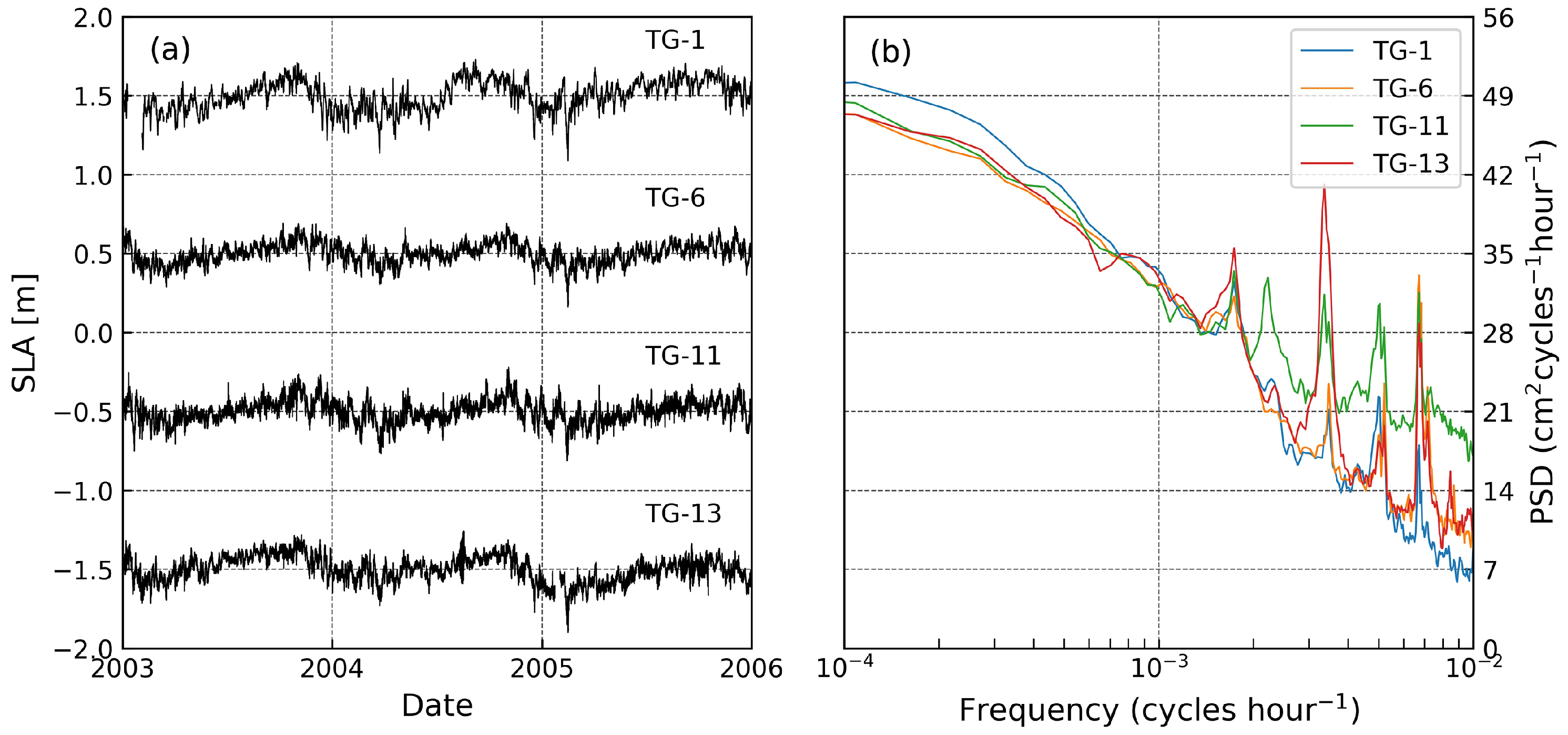
The time series of the de-tide and de-pressure sea level variability is described in Figure 3a to provide a good first look at the SLA spatial variability in the west Mediterranean Sea. It shows nearly consistent variations through 3 years, even though the mooring sites span in a different location (around 1200 km). This result indicates that TG signals are nearly uniform throughout the west Mediterranean Sea. Figure 3b shows that the TGs signals have revealed the high-frequency variations of the common mode signal at the period (T) between 3.5 to 27 days and the spectrum peak occurs at 0.003 cycles per hour (14 days). All of these high-frequency motion signals ( day) account for ~34.94% of the total change (Table 1). Such large energetic fluctuations can be explained by the unbalance of the mass exchange between the Atlantic and the Mediterranean Sea, which can lead to a high-frequency rise and fall through the west Mediterranean Sea as a whole [34]. It can contaminate the altimeter observations.
3.2. Non-Linear SLA Variations
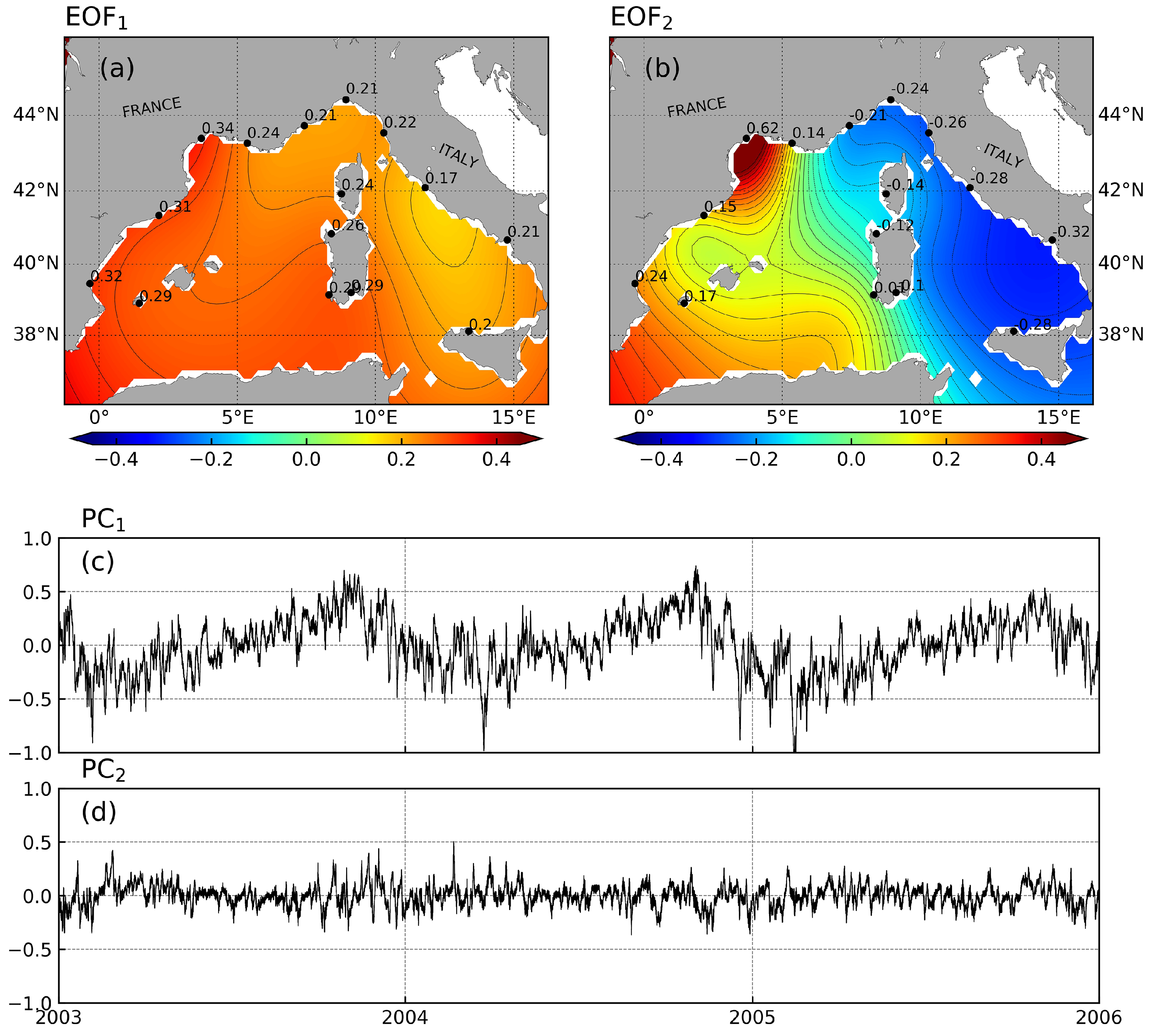
To extract the high-frequency large-scale fluctuations, the EOF analysis method was applied to the TGs-derived SLA over the wMWD to show up the time series of spatial-temporal fluctuations mapped by TGs in another way. Figure 4 shows the first two dominant components (EOF and EOF) of the EOF analysis results, which the spatial patterns were calculated by the Rbf interpolation method. In the 15 EOFs, the first five modes can account for about 90.03% of TGs SLA variances and the EOF (Figure 4a) accounts for about 67.9% of the total variance, explaining the spatial characteristic of the common mode signals. Only EOF1 has a spatial pattern that has the same sign throughout the wMED, it is consistent with the essential characteristics of the common mode (Figure 4a). The spatial pattern of EOF1 is not absolute uniform: the maximum (0.34) signal occurs in the Gulf of Lions and the minimal is in the Tyrrhenian Sea (0.17) and Ligurian Sea (0.20). This is understandable because the amplitude in the spatial pattern is modulated by the local shape and depth in the wMED, such as the strong currents in the Gulf of Lions and zonal wind stress immediately to the west of the straits [7,35,36]. The EOF explains 9.9% of the total variance and clearly shows an asymmetric oscillation like a “seesaw” with the axis of the two islands (Corsica and Sardinia). This phenomenon may be related to the island in the middle of wMED as discussed by Fukumori et al. [14].
The related temporal variation of EOF and EOF are shown in Figure 4c (PC) and Figure 4d (PC) respectively. They explaining the temporal features of large-scale fluctuations in the SLA. Time series of the PC has a standard deviation (Std.) of 0.26, and 0.10 for the PC. Although the spatial pattern of EOF has the sign, the difference of SLA between the west and east of the research area still reaches around 0.1 m in EOF, but in the spatial average method this value is 0. This illustrates an advantage the EOF analysis method over the spatial average method in the altimeter correction.
3.3. De-Aliasing of Jason1 and Envisat Data
We corrected the aliasing of the high-frequency common mode in Jason-1 and Envisat altimeter along-track SLA data in the wMED using the spatial average method and EOF analysis method. They calculated by the mean spatial TGs and EOF, respectively, and band-pass filtered them with a window of 2.5-2 days to correct altimetry SLA. In order to compare the two types of corrected method, the uncorrected and corrected Jason-1 and Envisat low-frequency variability of SLA grid data were interpolated to the position of TGs and compared with TGs data. The calculated PEL and COR results of two altimeters low-pass SLA data in two different correction methods with the 15 TGs (Figure 2) are listed in Table 2. In the EOF analysis method (EOF Corr.), 90% of the Jason-1 data at the TGs location has about 5% increase in COR, and ~3% increase for the Envisat data. Moreover, the mean PEL of Jason-1 reduced from 22.00% to 15.98%, and in Envisat reduced from 23.59% to 17.73%; these reductions accounted for about 30% of the total PEL. This result means that the EOF analysis method can improve the the low-frequency signal accuracy of SLA data in the wMED. In the spatial average correction method (Mean Corr.), only about 70% of Jason-1 and Envisat data at the TGs location has about 2% increase in COR. The remaining 30% of the data is reduced by about 3%. Moreover, the mean PEL in the Jason-1 and Envisat increased 4.10% and 3.53%, respectively, which increased PEL by about 20%. This indicates the PEL became worse after correction by averaging method. Both methods have an improvement for the TGs in the middle of the wMED (TGs No.1 and No.12–15) because the common mode in these places are less affected by the island and current. However, for the TG-4, TG-5, TG-8, TG-9, and TG-10, the SLA corrected by the TGs spatial average method may become worse. This might be related to the spatial pattern of EOF (Figure 4a), where the value of the EOF in the west and east of the wMED differs from mean EOF about and this difference can lead to errors in the spatial average method correction. The results indicate that the EOF method is better than the spatial average method for the common mode correction.
3.4. Difference in Correction Method
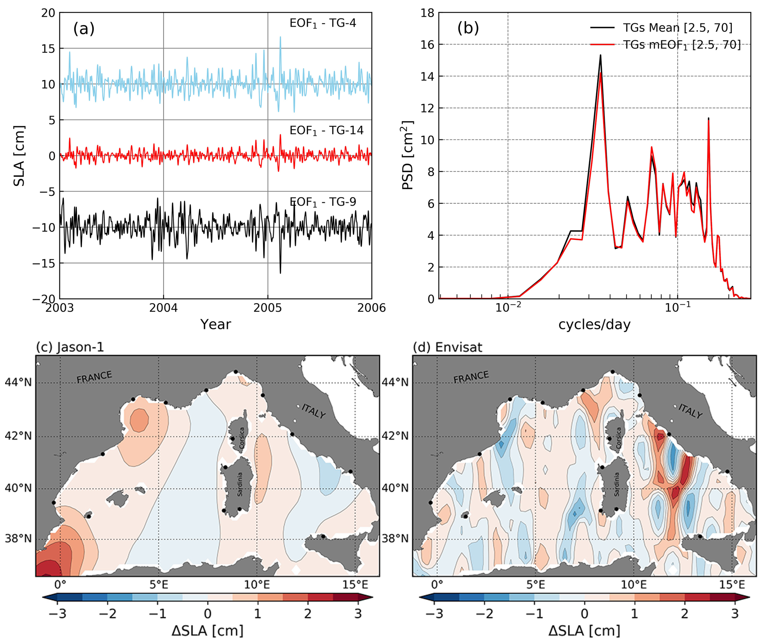
Figure 5a gives three examples of the 2.5 to 70 days band-pass filtered results of the common mode from the EOF at TG-4, TG-9, and TG-14. Comparing these three examples, significant changes of the common mode can be seen in spatial; the TG-14, in the middle of the wMED, has a standard deviation of 0.6 cm, which is lower than the standard deviation values of TG-4 (1.2 cm) and TG-9 (1.3 cm). The PSD of the spatial mean of EOF is in concordance with the spatial average result (Figure 5b). However, the spatial mean is neglecting local or regional information. Figure 5c,d shows why the EOF method has obtained better correction results. Their differences can reach about 3 cm. The difference between the EOF analysis method and spatial average method is larger in the regions where the eddies or the current are abundant (Figure 5c,d), such as Western Alborán grey, Thyrrhenian cyclonic circulation, and the Lions Gyre (see Figure 1).
4. Discussion
The altimeter SLA measurements have usually neglected the effect of the energetic non-tide high-frequency common mode signals in the marginal sea causing a significant aliasing errors in the gridded multiple altimeters SLA products. These aliasing errors will produce artificial mesoscale signals and even affect the interpretation of long-term oceanic/meteorological events [8,10]. As argued by Fukumori et al. [14], the non-tide, basin-wide and non-pressure-driven common mode signals have a period of 10 days to several years in the Mediterranean, and their amplitude can reach 10 cm. It suggests the urgent need of aliasing errors correction for the altimetry data.
We demonstrated an approach for tracking the common mode signals using the high-frequency TGs data to de-alias altimeter observations. This method consists of two main parts, the first step is based on the EOF method to extract the first mode (EOFPC) as the common mode signals. The second step is to remove the sub-sample high-frequency common mode ( days) from the altimeter along-track data. It is worked in the spacial and temporal for all altimeter along-track observations. In the west Mediterranean sea, the spatial characteristics of common mode signals are not absolute uniform, as shown in Figure 4a. This difference also proven in the energy of the fluctuations in Figure 3b. Therefore, the simple spatial average method [8,9] would introduce extra error in the altimeter correction.
The spatial variability of common mode signals may be related to the island in the middle of west Mediterranean, which delays the propagation of high-frequency signals to the entire basin (Figure 1) [7,15,35]. In the EOF analysis method, although only 15 TGs were used to the correction (Figure 2), more than 90% long period SLAs COR from Jason-1 and Envisat increase about 5% and 3%, respectively (Table 2), and better than the traditional spatial average method [9]. The EOF method was the most effective one in strong current areas. When the comparison was based on the PEL, the contaminate in the spatial average method is more pronounced, the percentage of PEL increased about 20%, especially in both sides of the basin. It is suggesting that the aliasing correction is space sensitive.
Comparing the corrected SLAs (Figure 5c,d), the difference between the two methods is more obvious in the Envisat correction. This is because the Envisat has a longer repeat cycle and more tracks [34]. It makes the aliasing in the Envisat more pronounce and the difference of the correction in the neighbor tracks more obvious. Meanwhile, it also reflects that this aliasing correction is time-sensitive. Therefore, our approach might provide new insights to correct the high-frequency barotropic signal errors in the altimeter data before mapping.
Although the corrected results seem to be good for the Jason-1 and Envisat gridded products, there are still some shortcomings in EOF method. One is that the extraction quality of the common mode signal is affected by the local signal, especially in the basin where there are islands, strong currents or near the sea strait [11,31]. They may impede the common signal transmission to the entire sea. For example, in the Japan Sea, the basin model caused by the shape of the basin can lead to a large difference in SLA between the north and south waters [37]. Even the EOF analysis method can overcome the shortcomings of space impact, the shape of the basin border, shallow water effect, and the processing errors in the TGs data, which need to be noted in the further analysis. Moreover, the accuracy of the EOF analysis method relies on the spatial distribution of TGs data. EOF analysis is classified as a multivariate statistical technique and it is difficult to distinguish different physical signals [11]. Despite these shortcomings, the PEL even increased after the correction by averaging method. It suggests that averaging method is not suitable for aliasing error correction in the wMED. The EOF analysis method described here can capture the common mode from the TGs data, and demonstrated the potential in altimeter data calibration. Therefore, the EOF method is the only method that can correct the aliasing errors of altimetry observations using TG data. This is of great practical significance because TG data is abundant and easily available in the global ocean. In the future, we will try to estimate the effect of different physical signals on the aliasing errors.
5. Conclusions
In this article, we have proposed a new effective method to extract the high-frequency barotropic signals in the wMED from TGs data to better correct the aliasing errors in the altimeter observations. We also analyzed the advantages and disadvantages of our method and compared with traditional methods in the altimeter along-track data correction using the wide distribution of 1 h TGs data. In the future, the long-term records and the wide distribution of 1 hour TGs data could be a reliable proxy for removing much common mode from past altimeter observations in the enclosed marginal seas. Moreover, the results of frequency analysis can be used to study the forces of the high-frequency basin fluctuation, such as wind, atmospheric pressure, and mass flux. This might improve our understanding of the ocean or meteorological simulate.
Author Contributions
D.H. designed the experiment and prepared the original draft. Y.X. contributed materials of remote sensing data and analysis models. All authors have read and agreed to the published version of the manuscript.
Funding
This work was supported by the National Key Research and Development Program (2016YFC1401004), Qingdao Pilot National Laboratory for Marine Science and Technology (2018ASKJ01), the National Natural Science Foundation of China (41676168, 41376028, 41421005, U1406401, 41906027), the National Key Research and Development Program (2019YFC1509102). Denghui Hu also acknowledges the Joint PhD Training financial support from the China Scholarship Council (CSC).
Acknowledgments
The authors also appreciate ESA for providing the Jason-1 and Envisat data via http://www.aviso.altimeter.fr and the tide gauge data from GESLA (Global Extreme Sea Level Analysis) project.
Conflicts of Interest
The authors declare no conflict of interest.
References
- Chent, G.; Ezraty, R. Alias impacts on the recovery of sea level amplitude and energy from altimeter measurements. Int. J. Remote Sens. 1996, 17, 3567–3576. [Google Scholar] [CrossRef]
- Mitchum, G.T. Comparison of TOPEX sea surface heights and tide gauge sea levels. J. Geophys. Res. Ocean. 1994, 99, 24541–24553. [Google Scholar] [CrossRef]
- Wang, J.; Fu, L.L.; Qiu, B.; Menemenlis, D.; Farrar, J.T.; Chao, Y.; Thompson, A.F.; Flexas, M.M. An observing system simulation experiment for the calibration and validation of the surface water ocean topography sea surface height measurement using in situ platforms. J. Atmos. Ocean. Technol. 2018, 35, 281–297. [Google Scholar] [CrossRef]
- Le Traon, P.; Nadal, F.; Ducet, N. An improved mapping method of multisatellite altimeter data. J. Atmos. Ocean. Technol. 1998, 15, 522–534. [Google Scholar] [CrossRef]
- Quinn, K.J.; Ponte, R.M. Estimating high frequency ocean bottom pressure variability. Geophys. Res. Lett. 2011, 38. [Google Scholar] [CrossRef]
- Larnicol, G.; Le Traon, P.Y.; Ayoub, N.; De Mey, P. Mean sea level and surface circulation variability of the Mediterranean Sea from 2 years of TOPEX/POSEIDON altimetry. J. Geophys. Res. Ocean. 1995, 100, 25163–25177. [Google Scholar] [CrossRef]
- Landerer, F.W.; Volkov, D.L. The anatomy of recent large sea level fluctuations in the Mediterranean Sea. Geophys. Res. Lett. 2013, 40, 553–557. [Google Scholar] [CrossRef]
- Xu, Y.; Watts, D.R.; Park, J.H. De-aliasing of large-scale high-frequency barotropic signals from satellite altimetry in the Japan/East Sea. J. Atmos. Ocean. Technol. 2008, 25, 1703–1709. [Google Scholar] [CrossRef] [Green Version]
- Li, H.; Xu, Y. Improving mesoscale observations from satellite altimetry using bottom pressure and tide gauge measurements in the Japan Sea. Int. J. Remote Sens. 2017, 38, 6247–6267. [Google Scholar] [CrossRef]
- Park, J.H.; Watts, D.R. Near-inertial oscillations interacting with mesoscale circulation in the southwestern Japan/East Sea. Geophys. Res. Lett. 2005, 32. [Google Scholar] [CrossRef] [Green Version]
- Preisendorfer, R. Principal component analysis in meteorology and oceanography. Elsevier Sci. Publ. 1988, 17, 425. [Google Scholar]
- Olita, A.; Ribotti, A.; Sorgente, R.; Fazioli, L.; Perilli, A. SLA–chlorophyll-a variability and covariability in the Algero-Provençal Basin (1997–2007) through combined use of EOF and wavelet analysis of satellite data. Ocean. Dyn. 2011, 61, 89–102. [Google Scholar] [CrossRef]
- Xi, H.; Losa, S.N.; Mangin, A.; Soppa, M.A.; Garnesson, P.; Demaria, J.; Liu, Y.; d’Andon, O.H.F.; Bracher, A. Global retrieval of phytoplankton functional types based on empirical orthogonal functions using CMEMS GlobColour merged products and further extension to OLCI data. Remote Sens. Environ. 2020, 240, 111704. [Google Scholar] [CrossRef]
- Fukumori, I.; Menemenlis, D.; Lee, T. A near-uniform basin-wide sea level fluctuation of the Mediterranean Sea. J. Phys. Oceanogr. 2007, 37, 338–358. [Google Scholar] [CrossRef] [Green Version]
- Ayoub, N.; Le Traon, P.Y.; De Mey, P. A description of the Mediterranean surface variable circulation from combined ERS-1 and TOPEX/POSEIDON altimetric data. J. Mar. Syst. 1998, 18, 3–40. [Google Scholar] [CrossRef]
- Cipollini, P.; Vignudelli, S.; Lyard, F.; Roblou, L. 15 years of altimetry at various scales over the Mediterranean. In Remote Sensing of the European Seas; Springer: Berlin/Heidelberg, Germany, 2008; pp. 295–306. [Google Scholar]
- Pinardi, N.; Masetti, E. Variability of the large scale general circulation of the Mediterranean Sea from observations and modelling: A review. Palaeogeogr. Palaeoclimatol. Palaeoecol. 2000, 158, 153–173. [Google Scholar] [CrossRef]
- Woodworth, P.L.; Hunter, J.R.; Marcos, M.; Caldwell, P.; Menéndez, M.; Haigh, I. Towards a global higher-frequency sea level dataset. Geosci. Data J. 2016, 3, 50–59. [Google Scholar] [CrossRef] [Green Version]
- Chen, G.; Lin, H. The effect of temporal aliasing in satellite altimetry. Photogramm. Eng. Remote Sens. 2000, 66, 639–644. [Google Scholar]
- Stammer, D.; Wunsch, C.; Ponte, R.M. De-aliasing of global high frequency barotropic motions in altimeter observations. Geophys. Res. Lett. 2000, 27, 1175–1178. [Google Scholar] [CrossRef] [Green Version]
- Schlax, M.G.; Chelton, D.B. Detecting aliased tidal errors in altimeter height measurements. J. Geophys. Res. Ocean. 1994, 99, 12603–12612. [Google Scholar] [CrossRef]
- Dee, D.P.; Uppala, S.M.; Simmons, A.; Berrisford, P.; Poli, P.; Kobayashi, S.; Andrae, U.; Balmaseda, M.; Balsamo, G.; Bauer, d.P.; et al. The ERA-Interim reanalysis: Configuration and performance of the data assimilation system. Q. J. R. Meteorol. Soc. 2011, 137, 553–597. [Google Scholar] [CrossRef]
- Dorandeu, J.; Le Traon, P. Effects of global mean atmospheric pressure variations on mean sea level changes from TOPEX/Poseidon. J. Atmos. Ocean. Technol. 1999, 16, 1279–1283. [Google Scholar] [CrossRef]
- Munk, W.H.; Cartwright, D.E. Tidal spectroscopy and prediction. Philos. Trans. R. Soc. Lond. Ser. A Math. Phys. Sci. 1966, 259, 533–581. [Google Scholar]
- Le Traon, P.; Faugère, Y.; Hernandez, F.; Dorandeu, J.; Mertz, F.; Ablain, M. Can we merge GEOSAT follow-on with TOPEX/Poseidon and ERS-2 for an improved description of the ocean circulation? J. Atmos. Ocean. Technol. 2003, 20, 889–895. [Google Scholar] [CrossRef]
- Berwin, R.W. JASON-1 Sea Surface High Anomaly Product User’s Reference Manual, Version 2; JPL Phys Oceanogr; DAAC: Pasadena, CA, USA, 2003. [Google Scholar]
- Carrère, L.; Lyard, F. Modeling the barotropic response of the global ocean to atmospheric wind and pressure forcing-comparisons with observations. Geophys. Res. Lett. 2003, 30. [Google Scholar] [CrossRef] [Green Version]
- Batoula Soussi, C. ENVISAT ALTIMETRY Level 2 User Manual. Envisat Altimetry Quality Working Group; ESA: Noordwijk, The Netherlands, 2011. [Google Scholar]
- Bretherton, F.P.; Davis, R.E.; Fandry, C. A technique for objective analysis and design of oceanographic experiments applied to MODE-73. In Deep Sea Research and Oceanographic Abstracts; Elsevier: Amsterdam, The Netherlands, 1976; Volume 23, pp. 559–582. [Google Scholar]
- Escudier, R.; Bouffard, J.; Pascual, A.; Poulain, P.M.; Pujol, M.I. Improvement of coastal and mesoscale observation from space: Application to the northwestern Mediterranean Sea. Geophys. Res. Lett. 2013, 40, 2148–2153. [Google Scholar] [CrossRef] [Green Version]
- Lorenz, E.N. Empirical Orthogonal Functions and Statistical Weather Prediction; MIT Department of Meteorology: Cambridge, MA, USA, 1956. [Google Scholar]
- Sharifi, M.; Forootan, E.; Nikkhoo, M.; Awange, J.; Najafi-Alamdari, M. A point-wise least squares spectral analysis (LSSA) of the Caspian Sea level fluctuations, using TOPEX/Poseidon and Jason-1 observations. Adv. Space Res. 2013, 51, 858–873. [Google Scholar] [CrossRef] [Green Version]
- López-Calderón, J.; Manzo-Monroy, H.; Santamaría-del Ángel, E.; Castro, R.; González-Silvera, A.; Millán-Núñez, R. Variabilidad de mesoescala del Pacífico tropical mexicano mediante datos de los sensores TOPEX y SeaWiFS. Cienc. Mar. 2006, 32, 539–549. [Google Scholar] [CrossRef]
- Vignudelli, S.; Cipollini, P.; Roblou, L.; Lyard, F.; Gasparini, G.; Manzella, G.; Astraldi, M. Improved satellite altimetry in coastal systems: Case study of the Corsica Channel (Mediterranean Sea). Geophys. Res. Lett. 2005, 32. [Google Scholar] [CrossRef]
- Poulain, P.M.; Menna, M.; Mauri, E. Surface geostrophic circulation of the Mediterranean Sea derived from drifter and satellite altimeter data. J. Phys. Oceanogr. 2012, 42, 973–990. [Google Scholar] [CrossRef]
- Bouzinac, C.; Font, J.; Johannessen, J. Annual cycles of sea level and sea surface temperature in the western Mediterranean Sea. J. Geophys. Res. Ocean. 2003, 108. [Google Scholar] [CrossRef] [Green Version]
- Xu, Y.; Watts, D.R.; Wimbush, M.; Park, J.H. Fundamental-mode basin oscillations in the Japan/East Sea. Geophys. Res. Lett. 2007, 34. [Google Scholar] [CrossRef] [Green Version]
Figure 1.
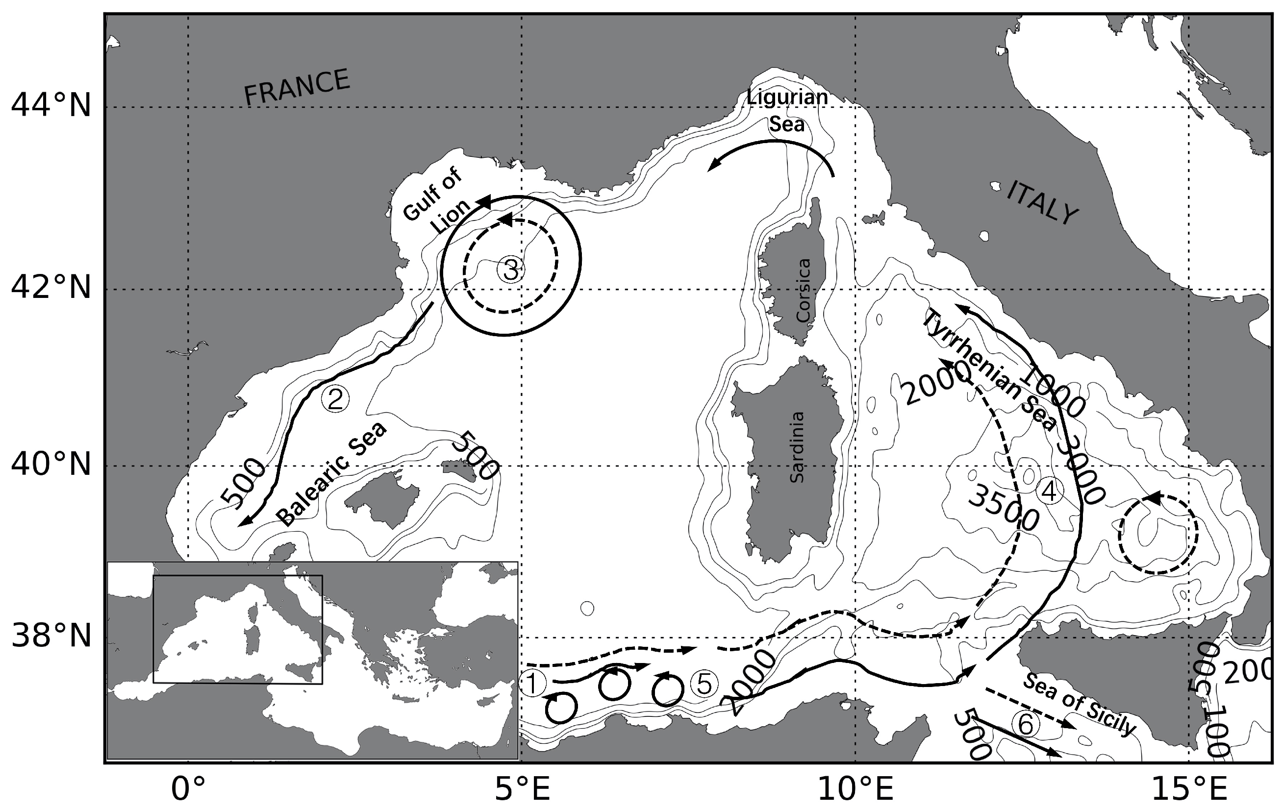
Map of main surface currents and eddies in the west Mediterranean Sea. Dashed arrows represent summer circulation, plain arrows represent winter circulation. ➀ Western Alborán gyre; ➁ Ligurian-Provençal current; ➂ Lions Gyre; ➃ Thyrrhenian cyclonic circulation with summer weakening and eastern anticyclone; ➄ Algerian current and eddies; ➅ Atlantic Ionian stream. Figure referenced from Pinardi and Masetti [17].
Figure 1.
Map of main surface currents and eddies in the west Mediterranean Sea. Dashed arrows represent summer circulation, plain arrows represent winter circulation. ➀ Western Alborán gyre; ➁ Ligurian-Provençal current; ➂ Lions Gyre; ➃ Thyrrhenian cyclonic circulation with summer weakening and eastern anticyclone; ➄ Algerian current and eddies; ➅ Atlantic Ionian stream. Figure referenced from Pinardi and Masetti [17].

Figure 2.
Locations of tide gauge (red squares) in the west Mediterranean Sea and the map of Envisat track (black square line) and Jason-1 track (gray square line).
Figure 2.
Locations of tide gauge (red squares) in the west Mediterranean Sea and the map of Envisat track (black square line) and Jason-1 track (gray square line).

Figure 3.
The left panel (a) shows the sea level anomaly (SLA) records after the de-tide and de-pressure processed at (TG-1): IBIZA, (TG-6): MONACO_PORT, (TG-11): PALERMO, and (TG-13): PORTO_TORRES. (b) The power spectral density (PSD) of the 4 TGs site.
Figure 3.
The left panel (a) shows the sea level anomaly (SLA) records after the de-tide and de-pressure processed at (TG-1): IBIZA, (TG-6): MONACO_PORT, (TG-11): PALERMO, and (TG-13): PORTO_TORRES. (b) The power spectral density (PSD) of the 4 TGs site.

Figure 4.
(a) The first EOFs of TGs sea level variability across the west Mediterranean Sea and (c) respond temporal amplitude. (b) The second EOFs of TGs sea level variability across the west Mediterranean Sea and (d) respond temporal amplitude. They accounted for 67.9% and 9.9% of non-tidal and non-atmospheric pressure corrected sea level variance within the basin, respectively. Colors denote the value of EOF spatial pattern. The black dot represents the location of TG sites.

Figure 5.
(a) A [2.5, 70] day band-pass filtered common mode calculated by the EOF at TG-4, TG-9 and TG-14. (b) The variance-preserving spectra of a [2.5, 70] day band-pass filtered common mode from the TGs by spatial average method (black line) and mean EOFs (red line). (c,d) The mean differences (color bar) of corrected SLA produced by spatial average method and EOF analysis method at Jason-1 and Envisat along-track data, respectively. The black dots stand for the location of TG sites.


Table 1.
Information of selected tide gauge stations. The last column indicates the percentage (Pct.) of high-frequency motion signals standard deviation (Std.).
Table 1.
Information of selected tide gauge stations. The last column indicates the percentage (Pct.) of high-frequency motion signals standard deviation (Std.).
| No. | St. Name | Longitude | Latitude | Record Pct. | Std. [cm] | Pct. of Std. () |
|---|---|---|---|---|---|---|
| 1 | IBIZA | 1.45 | 38.91 | 97.0% | 11.11 | 38.46% |
| 2 | VALENCIA | −0.33 | 39.46 | 99.6% | 10.98 | 39.06% |
| 3 | BARCELONA | 2.16 | 41.34 | 98.9% | 11.43 | 43.28% |
| 4 | SETE-SETE | 3.70 | 43.40 | 98.9% | 13.49 | 47.85% |
| 5 | MARSEILLE | 5.35 | 43.28 | 98.6% | 11.49 | 43.17% |
| 6 | MONACO_PORT | 7.42 | 43.73 | 100.0% | 11.04 | 34.47% |
| 7 | GENOVA | 8.93 | 44.41 | 96.1% | 11.57 | 35.35% |
| 8 | LIVORNO | 10.30 | 43.55 | 100.0% | 12.51 | 35.43% |
| 9 | CIVITAVECCHIA | 11.79 | 42.09 | 99.7% | 11.58 | 30.20% |
| 10 | SALERNO | 14.77 | 40.67 | 100.0% | 13.17 | 26.13% |
| 11 | PALERMO | 13.37 | 38.12 | 100.0% | 12.21 | 24.46% |
| 12 | AJACCIO_ASPRETTO | 8.76 | 41.92 | 84.5% | 11.93 | 33.80% |
| 13 | PORTO_TORRES | 8.40 | 40.84 | 99.0% | 11.44 | 31.67% |
| 14 | CARLOFORTE | 8.31 | 39.15 | 100.0% | 11.26 | 32.77% |
| 15 | CAGLIARI | 9.11 | 39.21 | 99.0% | 12.21 | 28.00% |
Table 2.
The PEL and COR of the difference between the long period ( low-pass) satellite altimeter SLAs and TG at 15 TG sites. The SLA were corrected with the spatial average method (Mean Corr.) or EOF analysis method (EOF Corr.).
Table 2.
The PEL and COR of the difference between the long period ( low-pass) satellite altimeter SLAs and TG at 15 TG sites. The SLA were corrected with the spatial average method (Mean Corr.) or EOF analysis method (EOF Corr.).
| TG Information | COR/PEL | TG-Jason1 20d Lowpass | TG-Envisat 70d Lowpass | |||||||
|---|---|---|---|---|---|---|---|---|---|---|
| No. | St. Name | Lon | Lat | (%) | Original | EOF Corr. | Mean Corr. | Original | EOF Corr. | Mean Corr. |
| 1 | IBIZA | 1.45 | 38.91 | COR | 87.83 | 89.24 | 88.51 | 90.14 | 90.88 | 90.57 |
| PEL | 18.77 | 14.04 | 17.58 | 13.34 | 14.03 | 13.4 | ||||
| 2 | VALENCIA | −0.33 | 39.46 | COR | 76.43 | 80.47 | 78.66 | 61.05 | 64.76 | 65.17 |
| PEL | 26.03 | 14.27 | 29.56 | 33.16 | 20.92 | 38.17 | ||||
| 3 | BARCELONA | 2.16 | 41.34 | COR | 83.93 | 85.78 | 84.26 | 85.71 | 87.13 | 86.52 |
| PEL | 22.33 | 14.79 | 28.64 | 21.76 | 15.45 | 28.1 | ||||
| 4 | SETE−SETE | 3.70 | 43.40 | COR | 79.33 | 83.68 | 73.68 | 80.37 | 83.74 | 78.40 |
| PEL | 22.05 | 15.91 | 30.03 | 21.47 | 13.36 | 29.51 | ||||
| 5 | MARSEILLE | 5.35 | 43.28 | COR | 84.37 | 86.49 | 85.16 | 73.77 | 74.35 | 73.78 |
| PEL | 16.85 | 13.06 | 22.53 | 19.07 | 16.04 | 20.13 | ||||
| 6 | MONACO_PORT | 7.42 | 43.73 | COR | 79.68 | 83.78 | 80.39 | 70.93 | 73.23 | 70.29 |
| PEL | 21.38 | 17.4 | 20.25 | 29.02 | 20.68 | 29.14 | ||||
| 7 | GENOVA | 8.93 | 44.41 | COR | 62.13 | 66.91 | 68.86 | 69.77 | 67.91 | 64.98 |
| PEL | 25.54 | 17.77 | 27.48 | 26.58 | 20.46 | 28.51 | ||||
| 8 | LIVORNO | 10.30 | 43.55 | COR | 82.00 | 83.83 | 76.75 | 73.03 | 75.60 | 70.98 |
| PEL | 16.12 | 10.27 | 25.92 | 19.66 | 12.28 | 28.57 | ||||
| 9 | CIVITAVECCHIA | 11.79 | 42.09 | COR | 65.01 | 67.97 | 62.83 | 74.71 | 77.78 | 70.34 |
| PEL | 24.64 | 17.2 | 31.62 | 20.56 | 14.89 | 29.94 | ||||
| 10 | SALERNO | 14.77 | 40.67 | COR | 50.90 | 58.25 | 48.93 | 48.85 | 50.37 | 46.86 |
| PEL | 30.89 | 18.77 | 40.57 | 33.1 | 17.37 | 42.86 | ||||
| 11 | PALERMO | 13.37 | 38.12 | COR | 83.24 | 88.69 | 80.32 | 72.74 | 71.18 | 64.26 |
| PEL | 26.1 | 19.93 | 29.75 | 29.06 | 20.43 | 35.59 | ||||
| 12 | AJACCIO_ASP... | 8.76 | 41.92 | COR | 88.37 | 89.99 | 88.49 | 87.31 | 87.50 | 87.01 |
| PEL | 19.03 | 15.59 | 22.05 | 25.02 | 23.26 | 27.93 | ||||
| 13 | PORTO_TORRES | 8.40 | 40.84 | COR | 88.96 | 87.75 | 86.92 | 78.35 | 80.17 | 81.85 |
| PEL | 20.87 | 22.45 | 19.02 | 21.32 | 17.39 | 17.28 | ||||
| 14 | CARLOFORTE | 8.31 | 39.15 | COR | 85.60 | 88.69 | 88.87 | 86.75 | 87.61 | 88.05 |
| PEL | 19.19 | 16.24 | 21.05 | 21.63 | 19.79 | 20.14 | ||||
| 15 | CAGLIARI | 9.11 | 39.21 | COR | 84.98 | 85.70 | 85.26 | 72.05 | 75.39 | 75.09 |
| PEL | 20.14 | 18.06 | 21.37 | 19.04 | 19.56 | 17.49 | ||||
© 2020 by the authors. Licensee MDPI, Basel, Switzerland. This article is an open access article distributed under the terms and conditions of the Creative Commons Attribution (CC BY) license (http://creativecommons.org/licenses/by/4.0/).
Share and Cite
MDPI and ACS Style
Hu, D.; Xu, Y. A New Method of De-Aliasing Large-Scale High-Frequency Barotropic Signals in the Mediterranean Sea. Remote Sens. 2020, 12, 2157. https://doi.org/10.3390/rs12132157
AMA Style
Hu D, Xu Y. A New Method of De-Aliasing Large-Scale High-Frequency Barotropic Signals in the Mediterranean Sea. Remote Sensing. 2020; 12(13):2157. https://doi.org/10.3390/rs12132157
Chicago/Turabian StyleHu, Denghui, and Yongsheng Xu. 2020. "A New Method of De-Aliasing Large-Scale High-Frequency Barotropic Signals in the Mediterranean Sea" Remote Sensing 12, no. 13: 2157. https://doi.org/10.3390/rs12132157
Note that from the first issue of 2016, this journal uses article numbers instead of page numbers. See further details here.