Hydrometeor Identification Using Multiple-Frequency Microwave Links: A Numerical Simulation


College of Meteorology and Oceanography, National University of Defense Technology, Nanjing 211101, China
*
Author to whom correspondence should be addressed.
Remote Sens. 2020, 12(13), 2158; https://doi.org/10.3390/rs12132158
Submission received: 18 June 2020
/
Revised: 1 July 2020
/
Accepted: 4 July 2020
/
Published: 6 July 2020
Abstract
:A method for identifying hydrometeor types (rain, graupel, and wet snow) based on a microwave link is proposed in this paper. The measured hydrometeor size distribution (HSD) data from the winters of 2014 to 2019 in Nanjing, China, were used to carry out simulation experiments to verify the performance of the model. Single-, dual-, and tri-frequency models (combinations of 15 GHz, 18 GHz, 25 GHz, 38 GHz, 50 GHz, 60 GHz, 70 GHz, and 80 GHz) were established with the extreme learning machine (ELM) algorithm. The results showed that the performance of the tri-frequency models was overall better than that of the dual-frequency models, for which the performance was better than that of the single-frequency models. The mean (maximum) test set accuracies of the single-frequency, dual-frequency, and tri-frequency models reached 75.8%, 80.7%, and 83.2% (83.0%, 84.4%, and 85.6%), respectively. For the dual-frequency and tri-frequency models, it was found that the accuracy increased with the overall frequency or the frequency difference. In addition, the influences of different noise levels on the model performance were also analyzed. Finally, the effects of position and length of link relative to precipitation cell were analyzed and are also discussed.
1. Introduction
Precipitation is an important research area in many fields of natural science [1,2,3]. In the water cycle, precipitation is the main way that water is transferred from the atmosphere to the ground [4]. Precipitation changes the salinity and temperature distribution of the upper ocean, further affecting the buoyancy of the ocean [5]. The erosion caused by precipitation is closely related to the evolution of landforms [6]. Therefore, the question of how to accurately monitor precipitation has always been a research focus. In recent years, researchers have been working on the improvement of precipitation-detection technology and have made considerable progress, e.g., the optical disdrometer [7,8,9], dual-polarized radar [10,11], spaceborne dual-frequency radar [12], etc. However, due to the complexity of and variability within the precipitation phenomenon itself, there are still obstacles to the accurate measurement of precipitation. Almost all the existing instruments and methods can only be said to have a good detection capability for certain types of hydrometeors, and it is difficult to fully consider the complexity of precipitation. To further improve the ability of precipitation monitoring under the condition of existing technologies, a feasible method is to identify hydrometeor types before making quantitative precipitation estimates. In addition, the identification of hydrometeor type is also of great significance for microwave communication. For example, when there is a melting layer in the air or melting snow near the ground, microwave signals will be seriously attenuated [13]. At such times, communication devices with an automatic transmission power control (ATPC) function will increase the transmission power to ensure normal communication.
A considerable amount of literature has been published on hydrometeor classification. There are two main ways to do this. One way is by in situ measurement. For example, Yuter et al. [14] separated the hydrometeors with the coexistence of rain and snow according to the velocity–size relationship measured by a Parsivel disdrometer. Praz et al. [15] developed an algorithm based on the geometric and texture features of hydrometeor images to identify six hydrometeor types and evaluated the degree of riming by multi-angle snowflake camera (MASC). The second way is microwave remote sensing. According to the polarization and attenuation characteristics under backscatter, polarimetric parameters (such as the reflectivity (ZH), differential reflectivity (ZDR), specific differential phase (KDP), linear depolarization ratio (LDR), and copolar correlation coefficient (ρHV)) of dual-polarized radar are used to identify hydrometeor types [16,17]. Hassan et al. [18] proposed a new fuzzy logic hydrometeor classification scheme applied to the French X-, C-, and S-Band polarimetric radars. Marzano et al. [19] estimated the type of hydrometeor from C-band dual-polarized radar by a Bayesian approach. Such methods can detect a wide range of precipitation, but the temporal and spatial resolution is limited, and it is difficult to represent near-surface precipitation due to the existence of radar elevation. Therefore, it is still a tremendous challenge to obtain information relating to hydrometeor types near the ground with a high spatial and temporal resolution.
In recent years, due to the low cost, wide distribution, representation of the real surface conditions, and other factors, the observation of precipitation via a terrestrial microwave link has gradually become an attractive research direction [3]. The basic principle is to retrieve the precipitation information according to the microwave attenuation caused by precipitation. The inversion of precipitation intensity [20] and the reconstruction of precipitation field [21] are the main areas that have been studied. In addition, this technique can be used as a supplement to weather radar measurements [22,23]. Furthermore, a few studies have begun to focus on dual-frequency [24] or dual-polarization [25] to inverse the hydrometeor size distribution (HSD). In fact, the attenuation of a multi-frequency dual-polarization microwave link also contains the information of hydrometeor type, which can be used to distinguish hydrometeor type. However, there have been few studies on the classification of hydrometeor based on microwave link. Holt et al. [26] studied the variations in the differential phase and attenuation of several precipitation processes at 12.8 GHz and 17.6 GHz, and indicated the potential of the differential phase for use in the recognition of snow and sleet. Cherkassky et al. [27] proposed a method to distinguish pure rain and sleet based on physical characteristics by using the receiving signal level of a commercial microwave link, which was tested with three links (18.36 GHz (vertical polarization), 19.37 GHz (horizontal and vertical polarization)). However, it only considered three hydrometeor types, pure rain, snow, and a mixture, and the data volume was small.
Unlike weather radar with several fixed frequencies (such as, S-, C-, or X-band), microwave links have multiple frequencies, ranging from several GHz to dozens of GHz. With the development of communication technology, even W-band (92–114.5 GHz) and D-band (141–174.8 GHz) microwave backhaul links may be used in the future, which will greatly stimulate the potential of microwave-link precipitation measurement. Compared with the classification of hydrometeor type based on dual-polarized radar that is widely used, the classification of hydrometeor type based on microwave link has the following advantages:
- The detection object reflects the real precipitation situation near the ground;
- Higher spatial and temporal resolution;
- It can be widely distributed in remote mountainous areas;
- It is low-cost, being based on commercial microwave communication equipment.
In order to explore the method of hydrometeor classification based on microwave links and make constructive suggestions for its practical application in the next step, this paper proposes a new method of hydrometeor-type identification via multiple-frequency microwave links. According to the frequency band of the typical microwave link, the identification results of hydrometeor types using microwave links with different frequency bands under different rain-cell conditions were investigated via numerical simulation. The major contributions of this paper are as follows: (1) A method to distinguish hydrometeor types based on the dual-polarization information of microwave links is proposed, and simulation experiments were carried out at single-frequency, dual-frequency and tri-frequency; (2) some criteria for frequency selection are suggested for future actual experimentation.
This paper is organized as follows: the next section analyzes the differences in the microphysical characteristics and the attenuation value distribution for different types of hydrometeors. Section 3 details the hydrometeor classification method and the microwave-link simulation experiment, while the performance of the various classification models and the influence of relative position and relative length of precipitation cell on it are analyzed in Section 4. In addition, several key issues are discussed in Section 5. Finally, the conclusion and summary are stated.
2. Microphysical Characteristics and Microwave Attenuations of Different Hydrometeors
2.1. Data Acquisition for Different Hydrometeors and the Properties of Hydrometeors
Due to their differences in physical characteristics, the V-D (velocity–diameter) relationships between different hydrometeors are obviously different [28]. Therefore, distinguishing hydrometeor types using the V-D relationship of hydrometeors obtained by statistics is a potential method that has been applied in certain studies [7,14]. Similarly, in this study, the V-D relationships observed by a Parsivel disdrometer (manufactured by OTT Messtechnik, Germany) were used to obtain samples of different types of hydrometeors. The data were from the winters of 2014 to 2019 in Nanjing, China, with a temporal resolution of 1 minute. In addition, the criterial V-D formula (see Table A1 in the Appendix A) for matching came from Locatelli et al. [29] and Atlas et al. [30], where the V-D empirical relationships of 14 solid hydrometeors and raindrops were fitted, respectively. The matching of hydrometeor type was based on the least square method:
where type represents the 15 hydrometeor types, Vtype refers to the V-D empirical formula of the type-type hydrometeor (for example, for hexagonal graupel, Vtype(D) = 1.10D0.57), V refers to the V-D empirical formula fitted with the disdrometer data, and n(i,j) refers to the number of hydrometeors recorded by the disdrometer for 1 minute at the ith size bin and the jth velocity bin (both size and velocity have 32 bins for Parsivel disdrometer). Furthermore, the 15 hydrometeor subclasses were further classified into three types: rain, graupel, and snow. Because of its distinct dielectric properties, snow was subdivided into dry snow and wet snow. The method used in this study was based on the temperature data observed on the ground: if the surface temperature at the time of obtaining the snow sample was greater than 0 °C, it was considered a wet snow sample; otherwise, it was considered a dry snow sample.
Through the above method, a total of 11,196 rain samples, 7521 graupel samples, 2014 dry snow samples and 545 wet snow samples were obtained. It is worth noting that the number of wet snow samples was too small. To balance the number of hydrometeor samples of different types, wet snow samples were oversampled using the SMOTE (Synthetic Minority Over-sampling Technique) method [31].
Raindrops, graupel particles, dry snow particles, and wet snow particles have different physical properties and dielectric properties due to their different formation mechanisms [28]. Raindrops are caused when droplets undergo the collision–coalescence process in clouds or when solid hydrometeors melt completely before falling to the ground [32]. The equivalent diameter of raindrops observed in nature is less than 8 mm [8]. When the equivalent diameter is less than 1 mm, the raindrop is considered to be a sphere, and when it is greater than 6 mm, it is considered to be an ellipsoid with an axial ratio of 0.7; between these shapes, the axial ratio of raindrop varies linearly from 1 to 0.7 with increasing equivalent diameter [33]. The relative dielectric constant of raindrops can be approximated as the complex dielectric constant of pure water . When the electromagnetic wave frequency range is 1 Hz to 3000 GHz, and can be expressed as [34]
where ε0 = 77.66 + 103.3(1 − t), fp = 20.20 + 146(1 − t) + (1 − t)2, fs = 39.8 × fp, t = 300/T, and T is the Kelvin temperature.
Graupel particles are nearly-spheroidal ice particles formed when supercooled water droplets come into contact with snow crystals and freeze on their surfaces. When the equivalent diameters are less than 1 mm, 1–4 mm, and 4–9 mm, the corresponding axial ratios are approximatively 1, 0.5, and 0.75, respectively [35]. The complex dielectric constant of ice can be calculated using the following formulas [36].
where α = (50.4 + 62θ) × 10−4e−22.1θ, β = (0.502 − 0.131θ)/(1 + θ) × 10−4 + 0.564 × 10⁻⁶(1 + θ)2/(0.0073 + θ)2, and θ = 300/T − 1.
Snow particles are the result of the deposition of vapor on the surface of ice crystals and of the aggregation between snowflakes and ice crystals [32]. Snow particles can be up to 15 mm in diameter and have complex shapes [37]. However, for snow particles less than 10 mm in diameter, the axial ratio is approximately 1. Meanwhile, for snow particles with a diameter greater than 10 mm, the axial ratio is approximately 0.9 [38]. The dielectric properties of snow particles are related to their water content. The complex dielectric constant of snow particles can be expressed as a function of the volume proportion of water W and form number u [39].
Typically, for dry snow, W = 0.05%, and u = 2; for wet snow, W = 3%, and u = 20.
2.2. Size Distribution of Hydrometeors
The hydrometeor size distribution (HSD) is commonly described by the gamma function [40];
where D (mm) is the equivalent diameter of the hydrometeor, N0 (mm−1 m−3) refers to the intercept parameter, μ (dimensionless) refers to the shape parameter, and Λ (mm−1) refers to the slope parameter. Nw (mm−1 m−3, normalized intercept parameter) and Dm (mm, mass-weighted mean diameter) reflect the overall concentration and size of hydrometeors, which can be calculated as
where is the nth moment. In addition, μ can be expressed as
where G = M43/(M6 M32). The liquid water equivalent precipitation rate in mm h−1 is equal to [41]
where V(D) (m s−1) and M(D) (g) are the fall speed and mass of the hydrometeor, respectively.
Figure 1 shows the distributions in the number concentrations of different types of hydrometeors relative to the diameter. As shown in this figure, the three kinds of non-liquid hydrometeors (graupel, wet snow, and dry snow) achieved a significantly larger size than raindrops did. At the same concentration, the diameter of dry snow was greater than that of wet snow, graupel, and rain (when N(D) < 1 mm−1 m−3). In addition, the HSDs of dry snow and wet snow were very similar except that, for the same diameter, the number concentration of wet snow was slightly lower than that of dry snow.
The probability distributions of log10Nw and Dm for the four types of hydrometeors are shown in Figure 2. The figure illustrates that the log10Nw values of rain and graupel (the mean values are 3.41 mm−1 m−3 and 3.30 mm−1 m−3, respectively) were larger than those of wet snow and dry snow (the mean values were 2.95 mm−1 m−3 and 2.99 mm−1 m−3, respectively) overall. The Dm values of dry snow, wet snow, and graupel (the mean values were 3.49 mm, 3.17 mm, and 2.58 mm, respectively) were obviously more inclined towards large values than rain was (the mean value for rain was 0.99 mm). This indicates that dry snow and wet snow have fewer particles but a larger size, whereas rain is the opposite, and graupel is somewhere in between. In addition, the mean values and standard deviations of the three parameters of HSD and precipitation rate are shown in Table 1.
2.3. Microwave Attenuations of Hydrometeors
The attenuation rate (dB/km) induced by hydrometeors can be expressed as [42]
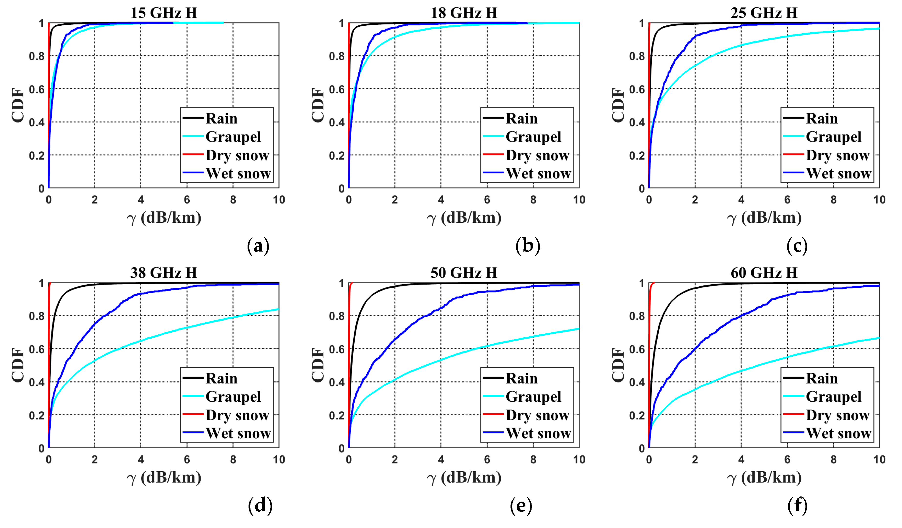
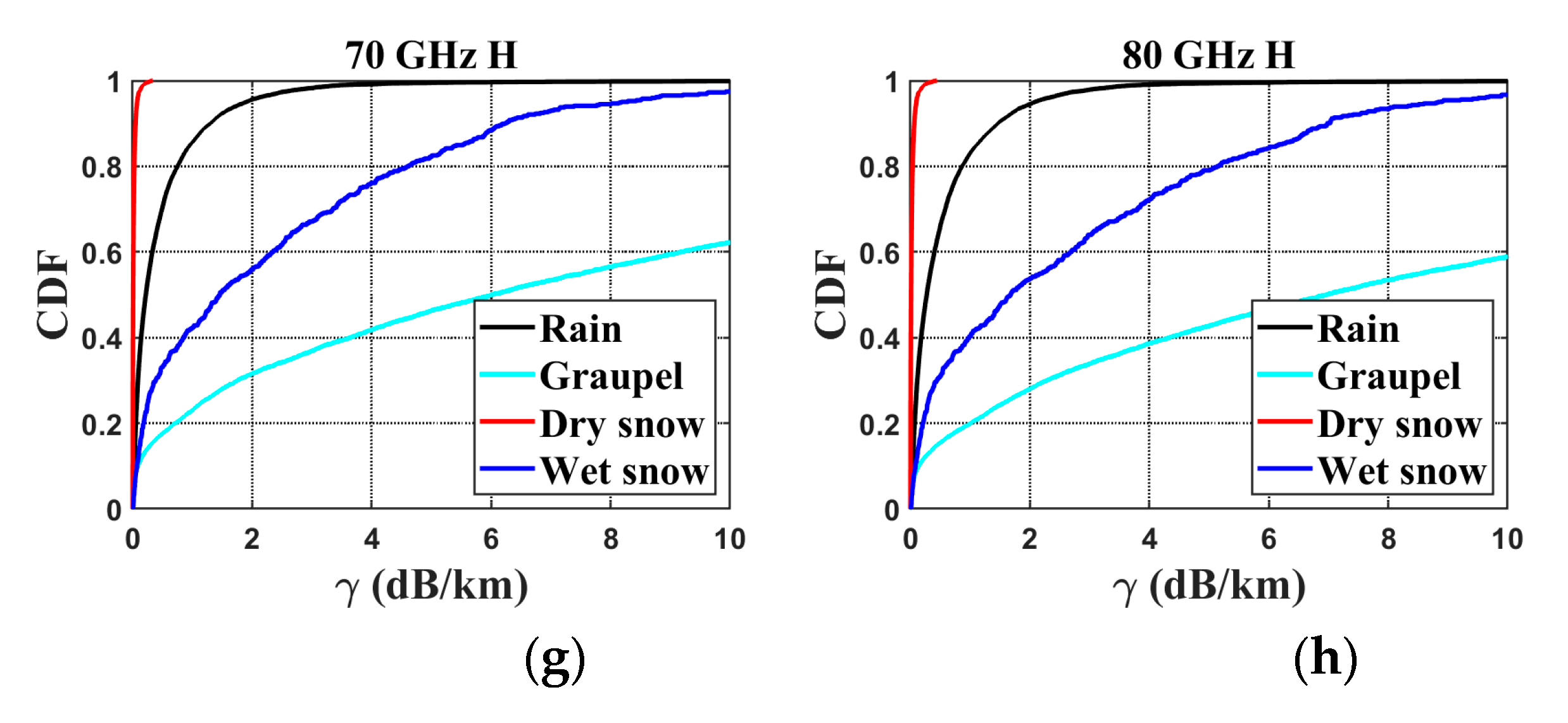
where f (GHz) is the electromagnetic frequency, and fH,V refers to the forward scattering amplitude at horizontal or vertical polarization. fH,V is calculated according to the T-matrix method [43], which is related to the shape and dielectric properties of the hydrometeor. Figure 3 shows the cumulative distribution function (CDF) of the attenuation values of the four types of hydrometeors at horizontal polarization for eight frequencies (common microwave link frequencies were selected in this study: 15 GHz, 18 GHz, 25 GHz, 38 GHz, 50 GHz, 60 GHz, 70 GHz, and 80 GHz) (the result was similar for vertical polarization, so it is not drawn here). As shown in this figure, the distribution range of graupel attenuation values was greater than that of wet snow, then greater than that of rain, and finally greater than that of dry snow for all frequencies. With the increase in frequency, the distribution difference of the attenuation values for different types of hydrometeors became increasingly obvious. This observation implies that the selection of precipitation attenuation at the highest possible frequency as a feature may lead to a better performance of the classification model. The above analysis indicated that the attenuation distribution characteristics of different types of hydrometeors exhibit diversity, and this diversity varies with the change in frequency, which verifies the potential of hydrometeor identification based on multiple-frequency microwave links.
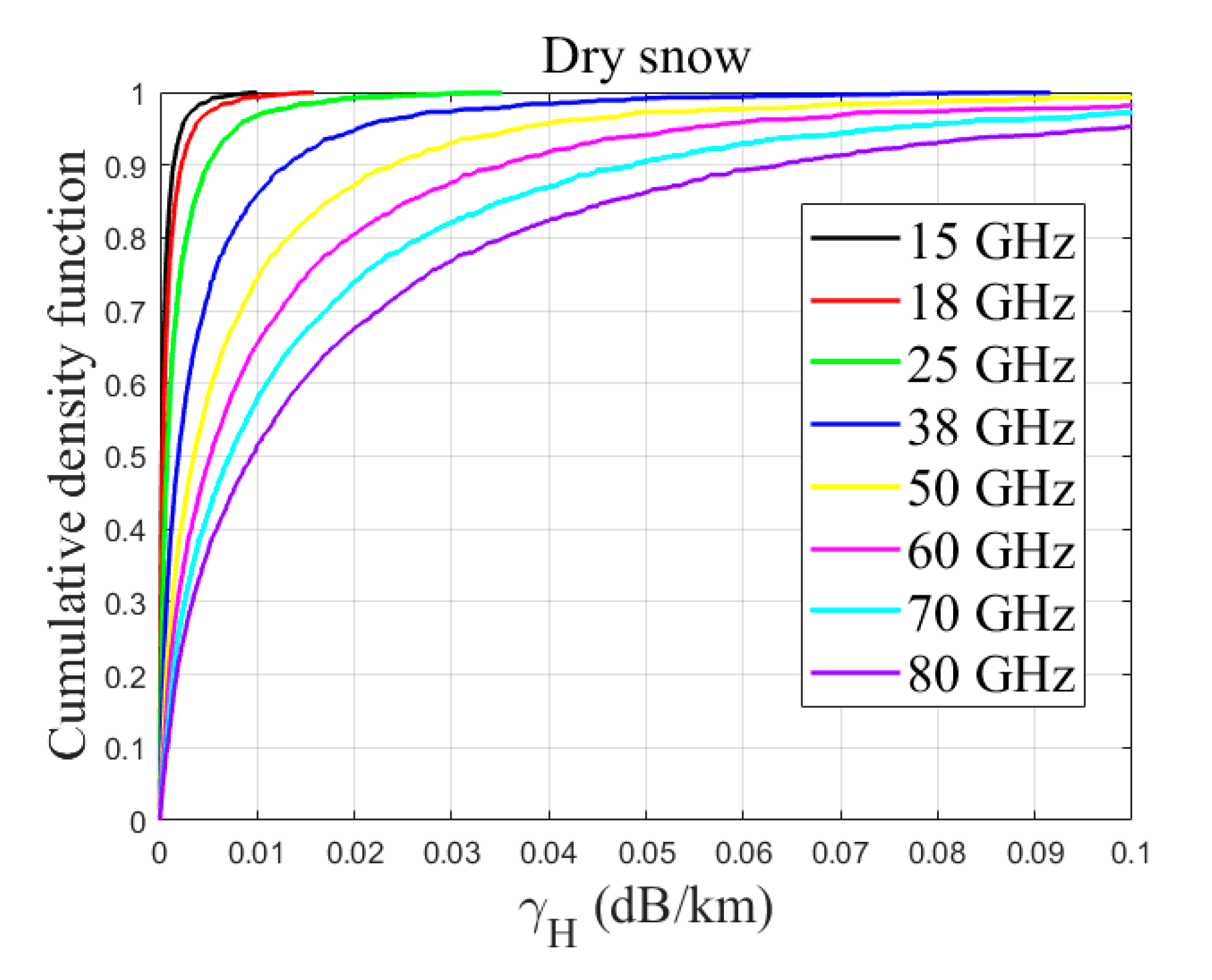
Figure 4 shows the cumulative density function of attenuation rates induced by dry snow at the horizontal polarization of eight frequencies. It is worth noting that the horizontal polarization attenuation rates of over 95% dry snow samples were less than 0.1 dB/km for all frequencies (even for 15 GHz, almost all of them were less than 0.01 dB/km). In addition, the microwave link also had quantization and random errors, which almost submerged the attenuation of dry snow. Therefore, it was almost impossible to identify dry snow by microwave attenuation (especially in regions with generally weak snowfall, such as eastern China), which was consistent with the measured results from Holt et al. [42]. In the following discussion, the objects of classification are the three types other than dry snow: rain, graupel, and wet snow.
3. Method of Hydrometeor Identification
3.1. Microwave Link Simulation
The purpose of this study was to optimize the frequency combination through simulation to provide a reference for future link design and experimentation. It was assumed that, for terrestrial link with horizontal path, the microwave receiver can receive microwave signals in the directions of horizontal and vertical polarizations. The total attenuation of the microwave over the terrestrial link with horizontal path is [3]
where (dB/km) is the average attenuation rate generated by the medium over the link at horizontal or vertical polarization and L (km) is the link length. The total microwave attenuation in the atmosphere is mainly composed of the following parts [44]:
where Aair is the dry air attenuation, Avapor is the vapor attenuation, Ahydro H,V is the hydrometeor attenuation at horizontal or vertical polarization, and Anoise is the attenuation associated with noise (due to the simulated experiment, the attenuation of a wet antenna was not considered). Aair and Avapor were calculated based on the ITU-R P.676-10 recommendation (taking into account data from winter and the general conditions in the Nanjing area, a temperature of 0 °C and an absolute humidity of 5.0 g m−3 were adopted). Suppose that Anoise = a × Gauss (Gauss represents the normal Gaussian distribution, and a stands for the noise coefficient) and a = 0.1 dB are set first (different noise levels are discussed later in Section 4) [45].
According to the observed HSDs corresponding to the different types of hydrometeors, the total attenuation value of each type of hydrometeor measured by the receiver can be obtained through Equation (13) (assuming that the level resolution of the receiver is 0.1 dB and the time resolution is 1 min). Hydrometeor attenuation can be calculated by removing the baseline value.
where the baseline value Abaseline H,V is the minimum value recorded by the receiver in the last 15 min [46]:
For the sake of simplicity, L was taken as 1 km in this study, and the average hydrometeor attenuation rate was .
3.2. Classification Method
Due to the differences in the axial ratio model and dielectric characteristics of different hydrometeors [28], the attenuation characteristics of microwaves at different polarization directions and frequencies are unique [45]. Therefore, the microwave attenuation information associated with a hydrometeor at different frequencies and polarization modes contains information of the hydrometeor type, which makes it possible to determine the hydrometeor type through microwave-link analysis. In this study, the attenuation values caused by a hydrometeor at the horizontal and vertical polarizations of a single frequency or multiple frequencies were extracted as the characteristic variable used to identify the hydrometeor type. The appropriate machine learning classification algorithm was then adopted for training (the ratio of test set samples to training set samples was 1:4), and the hydrometeor type recognition model was established and tested.
The classification algorithm used in this study was the extreme learning machine (ELM) (there may be some controversy about naming). ELM is an improved single-hidden-layer feedforward neural network, which has been widely used in regression and pattern recognition [47]. Compared with traditional algorithms (e.g., support vector machine (SVM) or single-layer perceptron), it has the advantages of a fast training speed and strong generalization ability. Assuming that the number of neurons in the input layer, hidden layer, and output layer is n (equal to the number of features), b, and m (equal to the number of types), the number of samples is N, and (xi, yi) is the ith sample (xi = [xi1, xi2,…, xin]T, yi = [yi1, yi2,…, yim]T). The process of model training is to make the output of the network as close as possible to the label
where oj= ; and are the weight vector and activation function of the ith hidden-layer neuron, respectively; and bi and wi are the bias and weight vector of the ith neuron connecting the input layer and the hidden layer, respectively. The key to model determination is to solve the following equation:
where H is the hidden-layer output matrix, β = [β1T, β2T,…, βbT]T, and Y = [y1T, y2T,…,yNT]T. H is a function of wi and bi, and is uniquely determined with random values of wi and bi. The training process of the ELM can then be simplified to the linear solution of β to determine the classification model. In addition, in order to show the superiority of the algorithm, the results based on decision tree (DT) [48] and probabilistic neural network (PNN) [49] classification algorithms are also shown in Section 4 for comparison.
4. Experimental Results
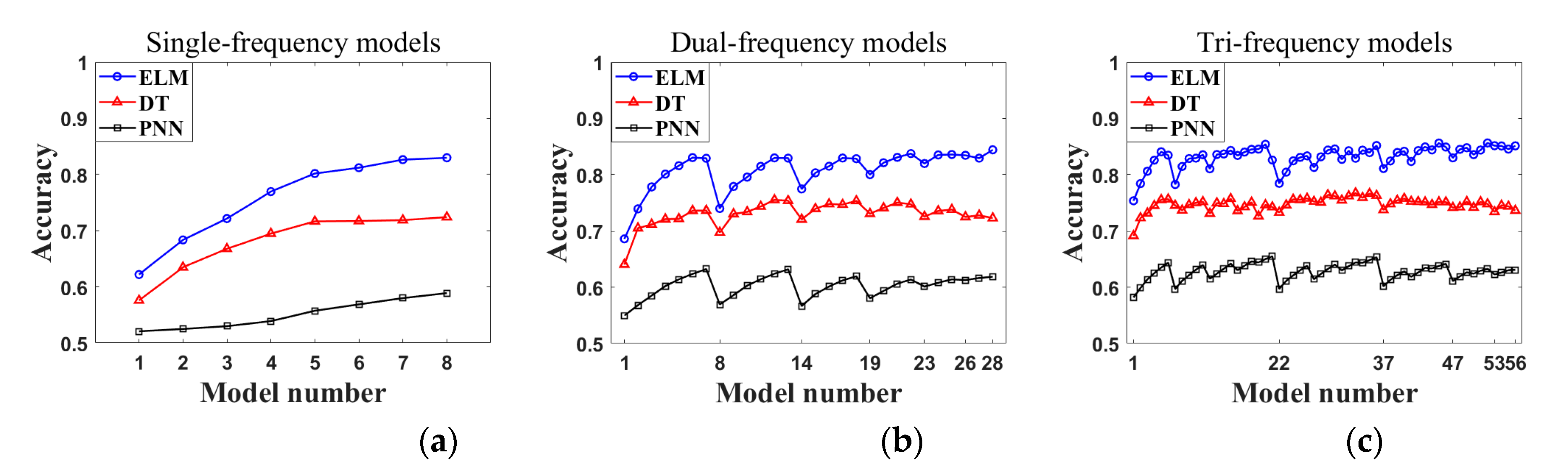
Combinations of one, two, or three of the frequencies 15 GHz, 18 GHz, 25 GHz, 38 GHz, 50 GHz, 60 GHz, 70 GHz, and 80 GHz were used, and the horizontal and vertically polarized hydrometeor attenuation rates of each frequency were used as feature variables. Figure 5 shows the scatter distributions of horizontal- and vertical-polarization attenuation rates for different types of hydrometeors at each frequency. As seen from the figure, compared with other types of hydrometeors, the attenuation difference between horizontal and vertical polarizations of graupel was more obvious. In addition, as the frequency increased, the dispersion of points became wider.
It was simply assumed that the length of all links was 1 km to facilitate the comparison of the effects of different frequencies on the performance of the classification model. However, in order to be closer to an actual situation, longer links were also simulated, and the differences in the relative length and relative position between them and the precipitation cell were also taken into account.
The accuracy was used to evaluate the performance of model. Assume that XY is the number of samples of hydrometeor type X that is classified as hydrometeor type Y, and rain, graupel, and wet snow are represented by A, B and C, respectively. The definition of accuracy was
The numbers of rain, graupel, and wet snow samples were 11,102, 7489, and 5984, respectively.
4.1. Single-Frequency Models
Figure 6a shows the test set accuracy of eight single-frequency models, and the model numbers are shown in Table 2. It can be seen that, for ELM, the accuracy of the model increased with the frequency, for which a possible reason is that low-frequency signals tend to be drowned out by noise. The model accuracies for frequencies of 50 GHz, 60 GHz, 70 GHz, and 80 GHz were all over 80% (80.2%, 81.2%, 82.6%, and 83.0%, respectively) and the mean test set accuracy of the single-frequency models was 75.8% for ELM. It is worth noting that the accuracy of the single-frequency model at high frequencies (especially at 80 GHz) could reach the same performance as the dual-frequency and tri-frequency models (as shown in Section 4.2 and Section 4.3). Therefore, if only a single-frequency microwave link is actually available, then the highest possible frequency should be selected. In addition, the results showed that the variation trend of different algorithms with model number was basically the same, but ELM was better than DT and then PNN on the whole (the difference in accuracy between the three algorithms was about 5–15% for the same model number). This indicated that the influence of different frequency combinations (model number) on the accuracy of classification results was relatively stable rather than random, and the overall performance can be improved through the improvement of algorithms (this was true not only for single-frequency models, but also for dual-frequency and tri-frequency models, as shown in Figure 6b,c. To avoid misunderstanding, all performance analyses in the following article refer to the ELM algorithm by default.
4.2. Dual-Frequency Models
Figure 6b presents the test set accuracies obtained from dual-frequency models. There were a total of 28 dual-frequency models, which were obtained by pairing the eight frequencies. The correspondence between frequency combinations and model numbers is shown in Table 3. Overall, for ELM, the accuracies of the dual-frequency models were higher than those of the single-frequency models (the mean and maximum accuracies of dual-frequency models were 80.7% and 84.4%, respectively). More than two-thirds of the models had an accuracy that was than 80% for ELM. In addition, the accuracy fluctuated obviously with the change in the model number. It is interesting to note that when one frequency was fixed while the other frequency was increasing, the accuracy of the model was constantly improved (e.g., from Model 1 to Model 7, Model 8 to Model 13, Model 14 to Model 18, and Model 19 to Model 22). Furthermore, the accuracy of the test set increased with the overall frequency (for example, the overall accuracy of Models 19–22 was higher than that of Models 14–18, which was higher than that of Models 8–13, which was finally higher than that of Models 1–7). This trend indicates that when a dual-frequency microwave link is used for hydrometeor type identification, the two frequencies should be selected with as much difference as possible or with as high an overall value as possible.
4.3. Tri-Frequency Models
It was found above that the performance of the dual-frequency models was improved compared with that of the single-frequency models. Therefore, this section discusses whether the accuracy of the tri-frequency models can be further improved. The test set accuracies of 56 tri-frequency models are shown in Figure 6c, and the corresponding frequency combinations are shown in Table 4. As shown in the figure, except for Models 1, 2, 7, and 22, the accuracies of the test sets of most models were above 80%, and the mean accuracy of all tri-frequency models was 83.2% for ELM. The accuracy reached a maximum of 85.6% at Model 52 for ELM. Similar to the dual-frequency models, the accuracies of the tri-frequency models fluctuate with the model number. However, compared with the dual-frequency models, the fluctuation range is relatively small. Except for a few irregular cases, the accuracy still increases with the overall frequency or frequency difference.
4.4. Precipitation Cell
Although in many cases we assumed that the precipitation field was evenly distributed within the detection range, this assumption obviously introduced great uncertainty relative to the scale of the microwave link. The typical size of a precipitation cell is 5–10 km [50]. For high-frequency links (for E-band, the link length may be less than 1 km, about 1/10 of the size), the length of precipitation cells may need less consideration. For the low-frequency links (where the link length may be more than ten kilometers or even twenty kilometers long), it is necessary to discuss the precipitation cell length.
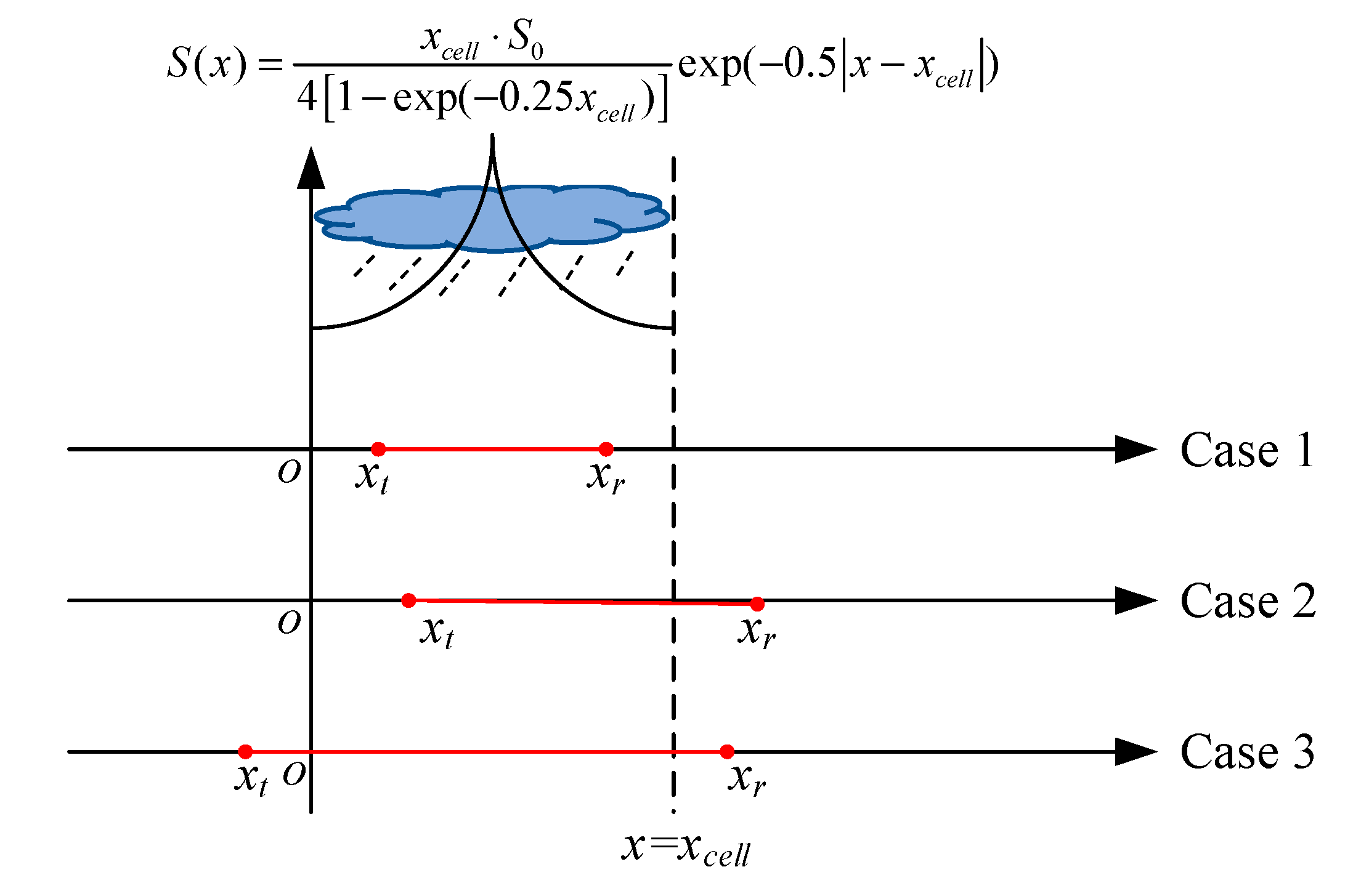
A well-known precipitation cell model is the EXCELL model [51], which assumes an exponential precipitation rate profile. Similarly, assuming an exponential distribution of surface precipitation rates,
where S1 (mm h−1) is the peak precipitation rate, x (km) is the position relative to the origin, xcell (km) is the peak position of precipitation cell, and c is the parameter associated with the effective scope of the cell. For the sake of discussion, the coordinate system shown in Figure 7 was defined. In order to control variables, the length of the precipitation cell was assumed to be 10 km, and only the influence of the location of the link relative to the precipitation cell and the length of the link on the classification model are analyzed below. Here, c was set to 0.5 (precipitation rate from the center of the cell to the boundary will be reduced to about 10%). Precipitation intensity S0 calculated from HSD data (according to Equation (9)) was used to determine the value of S1. Assuming that S0 represents the average precipitation rate of cell,
Thus, the value of S1 can be obtained:
for xcell = 10 km, S1 = 2.72 mm h−1. In addition, we used the HSD data obtained by disdrometer to fit the relationship between the Gamma parameters of different types of precipitation and the precipitation rate (see Table A2 in the Appendix A). Thus, according to an HSD sample, the HSD distribution of a precipitation cell can be obtained. Further, the locations of the link relative to the precipitation cell in three cases are shown in Figure 7. For Case 1 (0 < xt < xr < xcell, xt and xr represent the locations of the link transmitter and receiver, respectively), the link was completely within the coverage of the precipitation cell. For Case 2 (0 < xt < xcell < xr), one end of the link was outside the precipitation cell and the other was inside. For Case 3 (xt <0 < xcell < xr), both ends of the link were outside the precipitation cell. For each case, specific locations and lengths of different links were simulated and similar classification models ware established as above.
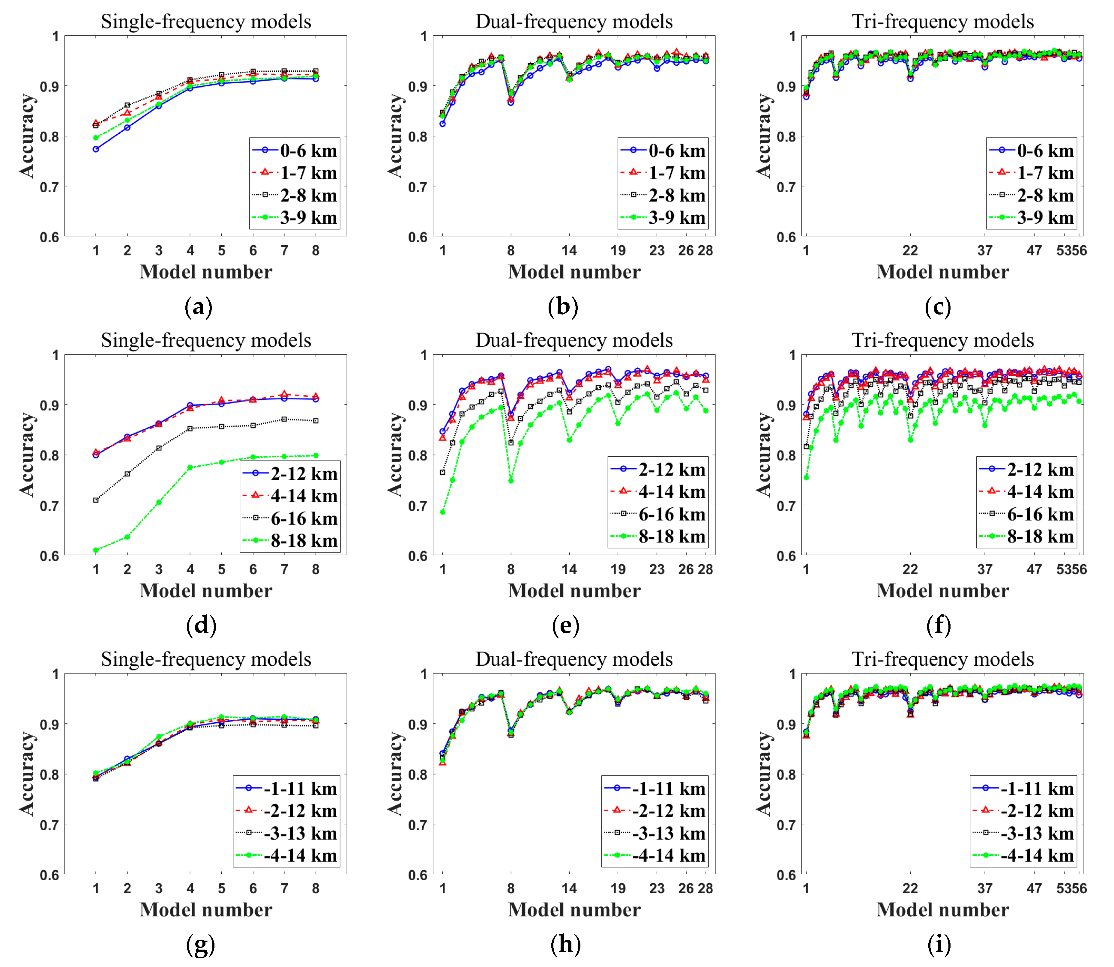
For Case 1, we assumed that the length of the link was 6 km, and the four location conditions relative to the precipitation cell were simulated ((xt, xr) was equal to (0, 6), (1, 7), (2, 8) and (3, 9), respectively, corresponding to getting closer and closer to the center of the precipitation cell) (as shown in Figure 8a–c. In general, due to the longer link length, the accuracies of the classification model were significantly improved (compared with those provided Section 4), no matter whether the model being used was a single-frequency, dual-frequency, or tri-frequency model (there are many combinations with accuracy greater than 95% in the dual-frequency and tri-frequency models). The increase of link length reduced the error, which corresponded to the analysis conclusion of Section 5.2. In addition, the trend of accuracy changing with the model number was basically unchanged (this was true not only for Case 1, but also for Cases 2 and 3, as shown in Figure 8d–i. Further, as the link came closer to the center of the precipitation cell (from 0–6 km to 1–7 km and then to 3–9 km), the accuracy of the model increased as a whole, but it decreased slightly as a whole when it was away from the precipitation cell (from 2–8 km to 3–9 km).
For Case 2, the length of the link was set to 10 km, and the four location conditions ((xt, xr) was equal to (2, 12), (4, 14), (6, 16), and (8, 18), respectively) were simulated, corresponding to getting farther and farther away from the precipitation cell) (as shown in Figure 8d–f). As the link was far away from the precipitation cell, the accuracy decreased on the whole, especially for 8–18 km, where only one fifth of the link was covered by precipitation cell. However, even in this case, the accuracies of some single-frequency models were still as high as 80%, and those of the dual-frequency and tri-frequency models were above 90%. As precipitation existed in only part of the links, the attenuation rate caused by precipitation as a feature variable was obviously reduced, but it still worked well, probably because the polarization information was introduced into the model. The potential relationships between precipitation-induced attenuation rates under horizontal and vertical polarization at different frequencies may be key to ensuring that the model can still maintain a good effect.
For Case 3, the precipitation cell waas completely contained within the link range, and the four location conditions ((xt, xr) was equal to (–1, 11), (–2, 12), (–3, 13), and (–4, 14), respectively) were simulated (as shown in Figure 8g–i). The results showed that the increase of link length had little effect on the accuracies of the models.
5. Discussion
5.1. Noise Levels
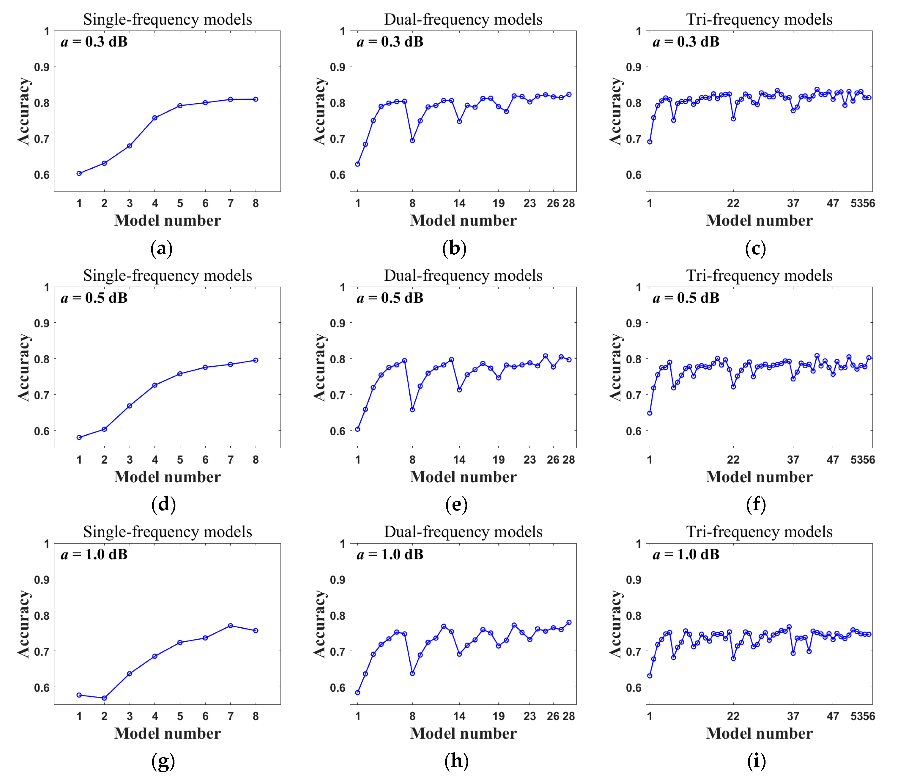
The previous analysis was based on a case where the noise coefficient a = 0.1 dB. However, the noise of an actual microwave link may be higher than this value, so it is necessary to discuss the noise level. Figure 9 shows the test set accuracies of the single-frequency, dual-frequency, and tri-frequency models with noise coefficients of 0.3 dB, 0.5 dB, and 1.0 dB. Whether using the single-frequency, dual-frequency, or tri-frequency model, the test set accuracy decreased with the increase in the noise coefficient. In addition, whether a = 0.1 dB, 0.3 dB, 0.5 dB, or 1.0 dB, the accuracy trends of the single-frequency, dual-frequency, and tri-frequency models’ changing with the model number were basically the same. When a = 0.3 dB, the mean accuracies of the single-frequency, dual-frequency, and triple-frequency models were 73.4%, 78.2%, 80.7%, and the maximum values were 80.8% (Model 8), 82.1% (Model 25), and 83.6% (Model 43). When a = 0.5 dB, regardless of whether the single-frequency, dual-frequency, or tri-frequency model was being used, there were still models with an accuracy greater than or equal to 80%. Even when a = 1.0 dB, models with an accuracy greater than 75% were still common, especially for tri-frequency models. In general, although the increase in noise level reduced the performance of classification models, effective models were still possible within the limited noise range.
5.2. Link Length and Link Data Processing
The actual length of commercial microwave links is not the same. Actually, it is related to carrier frequency. The atmosphere has a weak attenuation effect on low-frequency links, so the link length can be set very large (even up to tens of kilometers [52]). In contrast, a strong attenuation may occur on high-frequency links, so the link is generally set up short (even reaching the sub-kilometer level for the E-band [53]). The length of the link has its advantages and disadvantages. The actual value used for precipitation inversion is the attenuation rate caused by precipitation, which can be obtained by dividing the total attenuation caused by precipitation by the link length. Sufficient link length can reduce the error caused by instrument resolution. In addition, long links are relatively insensitive to the wet-antenna attenuation effect [53]. In contrast, short links are subject to baseline determination, wet-antenna attenuation, and receiving antenna resolution, especially for light rain. However, a short link length can make the spatial resolution of inversion results higher [53]. The link length of all frequencies was assumed in this study to be 1 km, which is less than the length of most actual microwave links. Therefore, better results can be expected for actual links.
The method used to process link data also has some influence on the inversion results. Firstly, if a rain gauge or disdrometer is not available, separation of dry and wet periods needs to be performed [54,55]. In addition, the water film covering the antenna surface can result in overestimation of the precipitation attenuation, and ice and snow in winter may also attach to it and cause similar effects [52]. Therefore, in the actual process, the appropriate wet-antenna calibration method is necessary. Unfortunately, although some studies have focused on wet-antenna correction during rainfall [56,57], due to its complexity, there are no generally accepted methods and conclusions, let alone for non-liquid precipitation.
5.3. Choice of Frequency
As shown in Section 4, different frequency combinations have a great impact on the accuracy of classification (the difference can be up to about 20%). For commercial microwave links, available frequency points are abundant but their distribution is uncertain. Therefore, it is necessary to select the optimal frequency combination for the existing hardware in the practical application process. Generally speaking, the more frequency combinations are selected, the more information they contain and the more favorable they may be for improving classification performance. However, considering the effect of actual link distribution density and noise, this may be impractical, especially for remote areas. If only one frequency can be obtained, the higher the frequency, the better the classification is likely to be. For dual-frequency models, as long as the combination contains 70 GHz or 80 GHz, the accuracies were basically stable at about 83%. Similarly, for the tri-frequency model, as long as the combination also contained 70 GHz or 80 GHz, the accuracies were basically stable at around 85%. In addition, the accuracies of single-frequency models at 70 GHz and 80 GHz were about 82%. This shows that for high-frequency links, the combination of multiple frequencies has little influence on them, and both single- and multi-frequency models can achieve ideal results. The performance improvement of multi-frequency combination is mainly reflected in low-frequency links. For example, the accuracy of a single-frequency model at 15 GHz was only 62.1%, but with the combination of 15 GHz and 18 GHz, the accuracy was increased to 68.6%, and the combination of 15 GHz, 18 GHz, and 25 GHz made it further increase to 75.3%. Coincidentally, most commercial microwave links currently operate at frequencies below 40 GHz, so it is expected that multi-frequency combinations for precipitation type differentiation will be meaningful. For the eight frequency points involved in this study, it is economical to select only a 70 GHz or 80 GHz single link if there is one. However, if a high frequency does not exist, a combination of several low-frequency links (such as 15 GHz, 18 GHz, 25 GHz, or 38 GHz) is beneficial, and the higher the overall frequency, the better the classification effect will be.
5.4. Hydrometeor Property
The properties of the assumed non-liquid hydrometeor were relatively ideal typical values, but in practice, these values are relatively volatile. For example, although the hypothesis of spherical snow particles can be applied to the scattering calculation [38], the shape of actual snow particles may be columnar, plate-like, needle-like, etc., which will inevitably introduce errors. In addition, in terms of dielectric property calculations, hydrometeors may not be uniform media; for example, wet snow particles may be surrounded externally by a layer of water. The differences in the description of particle microphysical characteristics and dielectric properties will cause errors in the calculation of scattering characteristics, which will have some influence on the simulation results. Of course, a more accurate description of hydrometeor properties depends on advances in observational techniques, such as the snowflake video imager (SVI)’s ability to record images of individual snowflakes [58], which will help to describe hydrometeor properties. However, SVI cannot measure falling speeds.
5.5. Classification Method
In this study, the data for different types of precipitation were obtained by matching the V-D relationships measured by Parsivel disdrometer with the empirical V-D relationships. On the one hand, the Parsivel disdrometer has errors in measuring V-D relationships. Although the radar reflectivity factor of snow measured by Parsivel disdrometer has good consistency with that measured by rain C-band radar [59], a Parsivel disdrometer is mainly used to measure the raindrop size distribution. The built-in algorithm assumes that the particles are spheres or ellipsoids, for which the equivalent diameter can be obtained by measuring the power weakened by the laser due to shielding, and the falling speed can be determined by the time the laser is shielded [60]. For non-liquid hydrometeors, such an algorithm is obviously not completely suitable. On the other hand, the empirical V-D relationships may not necessarily correspond to the actual local situations as encountered in different climatic zones. In addition, the falling velocity is also affected by real-time vertical airflow [28]. More advanced measuring instruments and classification methods are needed. For example, the types of hydrometeor can be determined using images taken by a multi-angle snowflake camera (MASC) [61]. Unfortunately, this device is still in the development stage, and its automated processing poses some challenges.
6. Conclusions and Prospects
In this paper, using HSD data measured by a Parsivel disdrometer, microwave link simulation experiments were carried out under different frequencies (15 GHz, 18 GHz, 25 GHz, 38 GHz, 50 GHz, 60 GHz, 70 GHz, and 80 GHz) and polarization modes (horizontal or vertical). The attenuation rates caused by rain, graupel, wet snow, and dry snow were calculated and used as feature variables to establish single-frequency, dual-frequency, and tri-frequency hydrometeor type identification models based on the ELM algorithm.
As the attenuation signal of dry snow was too weak, only rain, graupel, and wet snow were considered in the classification model. The classification results showed that, on the whole, the performance of the tri-frequency model was better than those of the dual-frequency model and the single-frequency model (the mean accuracies of the test sets were 83.2%, 80.7%, and 75.8%, and the highest accuracies are 85.6%, 84.4%, and 83.0%, respectively). For the dual-frequency and tri-frequency models, the accuracies were found to increase with the overall frequency or frequency difference. In addition, the performance of the model decreased with increases in noise level. When the noise coefficient was 0.5 dB, models with an accuracy greater than 80% still existed. When the noise factor was increased to 1.0 dB, there were still many models with an accuracy greater than 75%. Furthermore, the classification model achieved good performance under different precipitation cell and link combinations.
In addition to quantitative precipitation estimation, the identification of hydrometeor types using microwave links has become a hot research area. In this paper, a preliminary attempt was made to identify the hydrometeor type by using multi-frequency microwave links. In the future, measured link data will be collected to verify the simulations. However, there are still certain problems. For example, the problem of detecting dry snow remains difficult to solve using only attenuation information. However, it has been reported that the differential phase may be a good indicator for detecting dry snow [26], which is our next step. In addition, this study showed that the model classification effect obtained using high-frequency microwave links (60 GHz, 70 GHz, 80 GHz) was better than those obtained using low-frequency links, and these frequencies belong only to the frequency range of E-band commercial microwave links, which is a necessary part of the new generation of 5G networks. With further study of the E-band microwave link network, its potential in the field of hydrometeor type identification may be further explored in the future.
Author Contributions
Conceptualization, K.P. and X.L.; Formal analysis, K.P. and S.H.; Funding acquisition, X.L.; Methodology, K.P.; Project administration, X.L.; Resources, X.L. and T.G.; Supervision, X.L., S.H. and T.G.; Validation, K.P., X.L., S.H. and T.G.; Visualization, K.P.; Writing—original draft, K.P.; Writing—review & editing, K.P. and X.L. All authors have read and agree to the published version of the manuscript.
Funding
This research was funded by the National Science Foundation of China, grant number 41975030, 41505135 and 41475020.
Acknowledgments
The authors thank the anonymous reviewers and editors.
Conflicts of Interest
The authors declare no conflict of interest.
Appendix A

Table A1.
Empirical relationships of velocity (m/s)–diameter (mm) (V–D) and mass (mg)–diameter (mm) (M–D) for different types of precipitation. The empirical relationships of graupel and snow are derived from Locatelli and Hobbs [29]. The empirical relationships of rain are derived from Atlas et al. [30].
| Categories | Precipitation Type | V–D | M–D |
|---|---|---|---|
| Rain | Rain | V = 9.65 − 10.3exp(−0.6D) | M = π/6D3.0 |
| Graupel | Lump graupel 1 | V = 1.16D0.46 | M = 0.042D3.0 |
| Lump graupel 2 | V = 1.30D0.66 | M = 0.078D2.8 | |
| Lump graupel 3 | V = 1.50D0.37 | M = 0.140D2.7 | |
| Conical graupel | V = 1.20D0.65 | M = 0.073D2.6 | |
| Hexagonal graupel | V = 1.10D0.57 | M = 0.044D2.9 | |
| Snow | Graupellike snow of lump type | V = 1.10D0.28 | M = 0.059D2.1 |
| Graupellike snow of hexagonal type | V = 0.86D0.25 | M = 0.021D2.4 | |
| Densely rimed dendrites | V = 0.62D0.33 | M = 0.015D2.3 | |
| Densely rimed radiating assemblages | V = 1.10D0.12 | M = 0.039D2.1 | |
| Unrimed side planes | V = 0.81D0.99 | – | |
| Aggregates of unrimed radiating assemblages | V = 0.80D0.16 | M = 0.073D1.4 | |
| Aggregates of densely rimed radiating assemblages of dendrites or dendrites | V = 0.79D0.27 | M = 0.037D1.9 | |
| Aggregates of unrimed radiating assemblages of plates, side planes, bullets, and columns | V = 0.69D0.41 | M = 0.037D1.9 | |
| Aggregates of unrimed side planes | V = 0.82D0.12 | M = 0.040D1.4 |
Table A2.
The fitting relationship between the Gamma parameters (N0, u, Λ) and the precipitation rate S.
Table A2.
The fitting relationship between the Gamma parameters (N0, u, Λ) and the precipitation rate S.
| Categories | N0 = algS + b | u = aSb | Λ = aSb | |||
|---|---|---|---|---|---|---|
| a | b | a | b | a | b | |
| Rain | 150,882 | −3.89 | 4.42 | −0.28 | 7.31 | −0.36 |
| Graupel | 3279 | −0.65 | 1.21 | −0.53 | 2.09 | −0.37 |
| Wet snow | 38 | −1.59 | 1.40 | −0.38 | 0.85 | −0.46 |
| Dry snow | 965 | −0.256 | 1.02 | −0.43 | 1.11 | −0.34 |
References
- Nanko, K.; Moskalski, S.M.; Torres, R. Rainfall erosivity–intensity relationships for normal rainfall events and a tropical cyclone on the US southeast coast. J. Hydrol. 2016, 534, 440–450. [Google Scholar] [CrossRef] [Green Version]
- Michaelides, S. Precipitation: Advances in Measurement, Estimation and Prediction; Michaelides, S.C., Ed.; Springer: Berlin, Germany, 2008. [Google Scholar]
- Chwala, C.; Kunstmann, H. Commercial microwave link networks for rainfall observation: Assessment of the current status and future challenges. Wiley Interdiscip. Rev. Water 2019, 6. [Google Scholar] [CrossRef] [Green Version]
- Wang, A.; Zeng, X. Sensitivities of terrestrial water cycle simulations to the variations of precipitation and air temperature in china. J. Geophys. Res. Atmospheres 2011, 116. [Google Scholar] [CrossRef] [Green Version]
- Gosnell, R.; Fairall, C.W.; Webster, P.J. The sensible heat of rainfall in the tropical ocean. J. Geophys. Res. Ocean. 1995, 100, 18437–18442. [Google Scholar] [CrossRef]
- Masek, J.G.; Isacks, B.L.; Gubbels, T.L.; Fielding, E.J. Erosion and tectonics at the margins of continental plateaus. J. Geophys. Res. Solid Earth 1994, 99, 13941–13956. [Google Scholar] [CrossRef]
- Löffler–Mang, M.; Joss, J. An optical disdrometer for measuring size and velocity of hydrometeors. J. Atmos. Ocean. Technol. 2000, 17, 130–139. [Google Scholar] [CrossRef]
- Gatlin, P.N.; Thurai, M.; Bringi, V.N.; Petersen, W.; Wolff, D.; Tokay, A. Searching for Large Raindrops: A Global Summary of Two–Dimensional Video Disdrometer Observations. J. Appl. Meteorol. Climatol. 2015, 54, 1069–1089. [Google Scholar] [CrossRef]
- Minda, H.; Tsuda, N.; Fujiyoshi, Y. Three–Dimensional Shape and Fall Velocity Measurements of Snowflakes Using a Multiangle Snowflake Imager. J. Atmos. Ocean. Technol. 2017, 34, 1763–1781. [Google Scholar] [CrossRef]
- Thurai, M.; Gatlin, P.; Bringi, V.N.; Petersen, W.; Kennedy, P.; Notaroš, B.; Carey, L. Toward Completing the Raindrop Size Spectrum: Case Studies Involving 2D–Video Disdrometer, Droplet Spectrometer, and Polarimetric Radar Measurements. J. Appl. Meteorol. Climatol. 2017, 56, 877–896. [Google Scholar] [CrossRef]
- Bringi, V.N.; Williams, C.R.; Thurai, M.; May, P.T. Using Dual–Polarized Radar and Dual–Frequency Profiler for DSD Characterization: A Case Study from Darwin, Australia. J. Atmos. Ocean. Technol. 2009, 26, 2107–2122. [Google Scholar] [CrossRef]
- D’Adderio, L.P.; Vulpiani, G.; Porcù, F.; Tokay, A.; Meneghini, R. Comparison of GPM Core Observatory and Ground–Based Radar Retrieval of Mass–Weighted Mean Raindrop Diameter at Midlatitude. J. Hydrometeorol. 2018, 19, 1583–1598. [Google Scholar] [CrossRef]
- Upton, G.J.G.; Cummings, R.J.; Holt, A.R. Identification of melting snow using data from dual–frequency microwave links. IET Microw. Antennas Propag. 2007, 1. [Google Scholar] [CrossRef]
- Yuter, S.E.; Kingsmill, D.E.; Nance, L.B.; LÖffler–Mang, M. Observations of Precipitation Size and Fall Speed Characteristics within Coexisting Rain and Wet Snow. J. Appl. Meteorol. Climatol. 2006, 45, 1450–1464. [Google Scholar] [CrossRef] [Green Version]
- Praz, C.; Roulet, Y.-A.; Berne, A. Solid hydrometeor classification and riming degree estimation from pictures collected with a Multi–Angle Snowflake Camera. Atmos. Meas. Tech. 2017, 10, 1335–1357. [Google Scholar] [CrossRef] [Green Version]
- Snyder, J.C.; Bluestein, H.B.; Zhang, G.; Frasier, S.J. Attenuation Correction and Hydrometeor Classification of High–Resolution, X–band, Dual–Polarized Mobile Radar Measurements in Severe Convective Storms. J. Atmos. Ocean. Technol. 2010, 27, 1979–2001. [Google Scholar] [CrossRef]
- Schuur, T.; Park, H.-S.; Ryzhkov, A.V.; Reeves, H.D. Classification of Precipitation Types during Transitional Winter Weather Using the RUC Model and Polarimetric Radar Retrievals. J. Appl. Meteorol. Climatol. 2012, 51, 763–779. [Google Scholar] [CrossRef]
- Praz, C.; Roulet, Y.-A.; Berne, A. A New Fuzzy Logic Hydrometeor Classification Scheme Applied to the French X–, C–, and S–Band Polarimetric Radars. J. Appl. Meteorol. Climatol. 2013, 52, 2328–2344. [Google Scholar] [CrossRef]
- Marzano, F.S.; Scaranari, D.; Montopoli, M.; Vulpiani, G. Supervised Classification and Estimation of Hydrometeors From C–Band Dual–Polarized Radars: A Bayesian Approach. IEEE Trans. Geosci. Remote Sens. 2008, 46, 85–98. [Google Scholar] [CrossRef]
- Minda, H.; Nakamura, K. High Temporal Resolution Path–Average Rain Gauge with 50–GHz Band Microwave. J. Atmos. Ocean. Technol. 2005, 22, 165–179. [Google Scholar] [CrossRef]
- Goldshtein, O.; Messer, H.; Zinevich, A. Rain Rate Estimation Using Measurements From Commercial Telecommunications Links. IEEE Trans. Signal Process. 2009, 57, 1616–1625. [Google Scholar] [CrossRef]
- Rahimi, A.R.; Holt, A.R.; Upton, G.J.G. Attenuation Calibration of an X–band Weather Radar Using a Microwave Link. J. Atmos. Ocean. Technol. 2006, 23, 395–405. [Google Scholar] [CrossRef]
- Krämera, S.; Verworna, H.-R.; Redderb, A. Improvement of X–band Radar Rainfall Estimates Using a Microwave Link. Atmos. Res. 2005, 77, 278–299. [Google Scholar] [CrossRef]
- Rafael, F.R.; Roger, H.L. Microwave link dual–wavelength measurements of path–average attenuation for the estimation of drop size distributions and rainfall. IEEE Trans. Geosci. Remote Sens. 2002, 40, 760–770. [Google Scholar] [CrossRef]
- Berne, A.; Schleiss, M. Retrieval of the rain drop size distribution using telecommunication dual–polarization microwave links. In Proceedings of the 34th Conference on Radar Meteorology, Williamsburg, VA, USA, 5–9 October 2009. [Google Scholar]
- Holt, A.R.; Kuznetsov, G.G.; Rahimi, A.R. Comparison of the use of dual–frequency and single–frequency attenuation for the measurement of path–averaged rainfall along a microwave link. IET Microw. Antennas Propag. 2003, 150, 315. [Google Scholar] [CrossRef]
- Cherkassky, D.; Ostrometzky, J.; Messer, H. Precipitation Classification Using Measurements From Commercial Microwave Links. IEEE Trans. Geosci. Remote Sens. 2014, 52, 2350–2356. [Google Scholar] [CrossRef]
- Jia, X.; Liu, Y.; Ding, D.; Ma, X.; Chen, Y.; Bi, K.; Tian, P.; Lu, C.; Quan, J. Combining disdrometer, microscopic photography, and cloud radar to study distributions of hydrometeor types, size and fall velocity. Atmos. Res. 2019, 228, 176–185. [Google Scholar] [CrossRef]
- Locatelli, J.D.; Hobbs, P.V. Fall speeds and masses of solid precipitation particles. J. Geophys. Res. 1974, 79, 2185–2197. [Google Scholar] [CrossRef]
- Atlas, D.; Srivastava, R.C.; Sekhon, R.S. Doppler characteristics of precipitation at vertical incidence. Rev. Geophys. Space Phys. 1973, 11, 1–35. [Google Scholar] [CrossRef]
- Chawla, N.V.; Bowyer, K.W.; Hall, L.O.; Kegelmeyer, W.P. SMOTE: Synthetic minority over–sampling technique. J. Artif. Intell. Res. 2002, 16, 321–357. [Google Scholar] [CrossRef]
- Seela, B.K.; Janapati, J.; Lin, P.-L.; Wang, P.K.; Lee, M.-T. Raindrop Size Distribution Characteristics of Summer and Winter Season Rainfall Over North Taiwan. J. Geophys. Res. Atmos. 2018, 123, 11, 602–611, 624. [Google Scholar] [CrossRef] [Green Version]
- Chen, B.; Yang, J.; Pu, J. Statistical Characteristics of Raindrop Size Distribution in the Meiyu Season Observed in Eastern China. J. Meteorol. Soc. Jpn. Ser. II 2013, 91, 215–227. [Google Scholar] [CrossRef] [Green Version]
- Jiang, J.H.; Wu, D.L. Ice and water permittivities for millimeter and sub-millimeter remote sensing applications. Atmos. Sci. Lett. 2004, 5, 146–151. [Google Scholar] [CrossRef]
- Wang, W.; Liu, H.; Wang, G.; Pu, J.; Zhou, Z. Fundamentals of Atmospheric Science; China Meteorological Press: Beijing, China, 2011; Volume 5, p. 346. [Google Scholar]
- George, H. A model for the complex permittivity of ice at frequencies below 1 thz. Int. J. Infrared Millim. Waves 1991, 12, 677–682. [Google Scholar] [CrossRef]
- Pruppacher, H.R.; Klett, J.D. Cloud processes (book reviews: Microphysics of clouds and precipitation). Science 1979, 204, 381–382. [Google Scholar] [CrossRef]
- Oguchi, T. Electromagnetic wave propagation and scattering in rain and other hydrometeors. Proc. IEEE 1983, 71, 1029–1078. [Google Scholar] [CrossRef]
- Awaka, J.; Furuhama, Y.; Hoshiyama, M.; Nishitsuji, A. Model calculations of scattering properties of spherical bright–band particles made of composite dielectrics. Proc. J. Radio Res. Lab. Jpn. 1985, 32, 73–87. [Google Scholar]
- Niu, S.; Jia, X.; Sang, J.; Liu, X.; Lu, C.; Liu, Y. Distributions of Raindrop Sizes and Fall Velocities in a Semiarid Plateau Climate: Convective versus Stratiform Rains. J. Appl. Meteorol. Climatol. 2010, 49, 632–645. [Google Scholar] [CrossRef]
- Boudala, F.S.; Isaac, G.A.; Rasmussen, R.; Cober, S.G.; Scott, B. Comparisons of Snowfall Measurements in Complex Terrain Made During the 2010 Winter Olympics in Vancouver. Pure Appl. Geophys. 2014, 171, 113–127. [Google Scholar] [CrossRef]
- Holt, A.R.; Cummings, R.J.; Upton, G.J.G.; Bradford, W.J. Rain rates, drop size information, and precipitation type, obtained from one–way differential propagation phase and attenuation along a microwave link. Radio Sci. 2008, 43, 1–18. [Google Scholar] [CrossRef]
- Mishchenko, M.I.; Videen, G.; Babenko, V.A.; Khlebtsov, N.G.; Wriedt, T. T–matrix theory of electromagnetic scattering by partciles and its applications: A comprehensive reference database. J. Quant. Spectrosc. Radiat. Transfer 2004, 88, 357–406. [Google Scholar] [CrossRef]
- Zinevich, A.; Messer, H.; Alpert, P. Prediction of rainfall intensity measurement errors using commercial microwave communication links. Atmos. Meas. Tech. Tech. 2010, 3, 1385–1402. [Google Scholar] [CrossRef] [Green Version]
- Pu, K.; Liu, X.; Xian, M.; Gao, T. Machine Learning Classification of Rainfall Types Based on the Differential Attenuation of Multiple Frequency Microwave Links. IEEE Trans. Geosci. Remote Sens. 2020, 58, 1–12. [Google Scholar] [CrossRef]
- Ostrometzky, J.; Messer, H. Dynamic Determination of the Baseline Level in Microwave Links for Rain Monitoring From Minimum Attenuation Values. IEEE Sel. Top. Appl. Earth Obs. Remote Sens. 2018, 11, 24–33. [Google Scholar] [CrossRef]
- Huang, G.-B.; Zhu, Q.-Y.; Siew, C.-K. Extreme learning machine: Theory and applications. Neurocomputing 2006, 70, 489–501. [Google Scholar] [CrossRef]
- Safavian, S.R.; Landgrebe, D. A survey of decision tree classifier methodology. IEEE Trans. Syst. Man Cybern. 1991, 21, 660–674. [Google Scholar] [CrossRef] [Green Version]
- Mao, K.Z.; Tan, K.C.; Ser, W. Probabilistic neural–network structure determination for pattern classification. IEEE Trans. Neural Netw. 2000, 11, 1009–1016. [Google Scholar] [CrossRef] [Green Version]
- Emanuel, K.A. On the Dynamical Definition(s) of “Mesoscale”. In Mesoscale Meteorology—Theories, Observations and Models; Springer: Dordrecht, The Netherlands, 1983; Volume 114, pp. 1–11. [Google Scholar]
- Luini, L.; Capsoni, C. A Rain Cell Model for the Simulation and Performance Evaluation of Site Diversity Schemes. IEEE Antennas Wirel. Propag. Lett. 2013, 12, 1327–1330. [Google Scholar] [CrossRef]
- Maximilian, G.; Christian, C.; Julius, P.; Harald, K. Rainfall estimation from a German–wide commercial microwave link network: Optimized processing and validation for one year of data. Hydrol. Earth Syst. Sci. 2019. [Google Scholar] [CrossRef] [Green Version]
- Fencl, M.; Dohnal, M.; Valtr, P.; Grabner, M.; Bareš, V. Atmospheric observations with E–band microwave links—Challenges and opportunities. Atmos. Meas. Tech. 2020. [Google Scholar] [CrossRef] [Green Version]
- Schleiss, M.; Berne, A. Identification of Dry and Rainy Periods Using Telecommunication Microwave Links. IEEE IEEE Geosci. Remote Sens. Lett. 2010, 7, 611–615. [Google Scholar] [CrossRef]
- Wang, Z.; Schleiss, M.; Jaffrain, J.; Berne, A.; Rieckermann, J. Using Markov switching models to infer dry and rainy periods from telecommunication microwave link signals. Atmos. Meas. Tech. 2012, 5, 1847–1859. [Google Scholar] [CrossRef] [Green Version]
- Moroder, C.; Siart, U.; Chwala, C.; Kunstmann, H. Modeling of Wet Antenna Attenuation for Precipitation Estimation From Microwave Links. IEEE Geosci. Remote Sens. Lett. 2019, 17, 386–390. [Google Scholar] [CrossRef]
- Schleiss, M.; Rieckermann, J.; Berne, A. Quantification and Modeling of Wet–Antenna Attenuation for Commercial Microwave Links. IEEE Geosci. Remote Sens. Lett. 2013, 10, 1195–1199. [Google Scholar] [CrossRef]
- Newman, A.J.; Kucera, P.A.; Bliven, L.F. Presenting the Snowflake Video Imager (SVI). J. Atmos. Ocean. Technol. 2009, 26, 167–179. [Google Scholar] [CrossRef]
- Löffler-Mang, M.; Blahak, U. Estimation of the Equivalent Radar Reflectivity Factor from Measured Snow Size Spectra. J. Atmos. Ocean. Technol. 2001, 40, 843–849. [Google Scholar] [CrossRef]
- Battaglia, A.; Rustemeier, E.; Tokay, A.; Blahak, U.; Simmer, C. PARSIVEL Snow Observations: A Critical Assessment. J. Atmos. Ocean. Technol. 2010, 27, 333–344. [Google Scholar] [CrossRef]
- Garrett, T.J.; Yuter, S.E.; Fallgatter, C.; Shkurko, K.; Rhodes, S.R.; Endries, J.L. Orientations and aspect ratios of falling snow. Geophys. Res. Lett. 2015, 42, 4617–4622. [Google Scholar] [CrossRef]
Figure 1.
Mean hydrometeor size distributions (HSDs) of rain (black), graupel (cyan), wet snow (red), and dry snow (blue).
Figure 1.
Mean hydrometeor size distributions (HSDs) of rain (black), graupel (cyan), wet snow (red), and dry snow (blue).

Figure 2.
The probability histograms of the normalized intercept parameters log10Nw (mm−1m−3) (a,c,e,g) and mass-weighted mean diameters Dm (mm) (b,d,f,h) for rain, graupel, wet snow, and dry snow, respectively.
Figure 2.
The probability histograms of the normalized intercept parameters log10Nw (mm−1m−3) (a,c,e,g) and mass-weighted mean diameters Dm (mm) (b,d,f,h) for rain, graupel, wet snow, and dry snow, respectively.

Figure 3.
Cumulative distribution functions (CDFs) of horizontal-polarization attenuation rates induced by hydrometeors with frequencies of (a) 15 GHz, (b) 18 GHz, and (c) 25 GHz, (d) 38 GHz, (e) 50 GHz, (f) 60 GHz, (g) 70 GHz, and (h) 80 GHz for rain (black), graupel (cyan), wet snow (red), and dry snow (blue).


Figure 4.
Cumulative density curves for the horizontal-polarization attenuation rates of dry snow at 15 GHz, 18 GHz, 25 GHz, 38 GHz, 50 GHz, 60 GHz, 70 GHz, and 80 GHz.
Figure 4.
Cumulative density curves for the horizontal-polarization attenuation rates of dry snow at 15 GHz, 18 GHz, 25 GHz, 38 GHz, 50 GHz, 60 GHz, 70 GHz, and 80 GHz.

Figure 5.
Scatter plots of horizontally and vertically polarized hydrometeor-induced attenuation pairs at frequencies of (a) 15 GHz, (b) 18 GHz, and (c) 25 GHz, (d) 38 GHz, (e) 50 GH, (f) 60 GHz, (g) 70 GHz, and (h) 80 GHz for rain (black square), graupel (cyan point), dry snow (red star), and wet snow (blue triangle).

Figure 6.
Test set accuracy of the ELM, DT, and PNN for (a) single-frequency, (b) dual-frequency, and (c) tri-frequency models, respectively.
Figure 6.
Test set accuracy of the ELM, DT, and PNN for (a) single-frequency, (b) dual-frequency, and (c) tri-frequency models, respectively.

Figure 7.
The schematic diagram of the precipitation cell model and link distribution under three cases.
Figure 7.
The schematic diagram of the precipitation cell model and link distribution under three cases.

Figure 8.
Test set accuracy of the ELM for single-frequency, dual-frequency, and tri-frequency models in three cases. (a–c) represent the single-frequency, dual-frequency, and triple-frequency models for Case 1, respectively. (d–f) represent the single-frequency, dual-frequency, and triple-frequency models for Case 2, respectively. (g–i) represent the single-frequency, dual-frequency, and triple-frequency models for Case 3, respectively.

Figure 9.
Test set accuracy of the ELM for single-frequency, dual-frequency, and tri-frequency models. (a–c) represent the single-frequency, dual-frequency, and triple-frequency models for a = 0.3 dB, respectively. (d–f) represent the single-frequency, dual-frequency, and triple-frequency models for a = 0.5 dB, respectively. (g–i) represent the single-frequency, dual-frequency, and triple-frequency models for a = 1.0 dB, respectively.

Table 1.
The mean (standard deviation) of the four parameters of rain, graupel, wet snow, and dry snow.
Table 1.
The mean (standard deviation) of the four parameters of rain, graupel, wet snow, and dry snow.
| Parameter | Rain | Graupel | Wet Snow | Dry Snow |
|---|---|---|---|---|
| Precipitation rate S (mm/h) | 0.73 (2.55) | 2.07 (2.93) | 0.16 (0.20) | 0.27 (0.40) |
| Shape parameter μ | 7.58 (6.35) | 2.90 (4.98) | 4.79 (4.49) | 4.10 (5.38) |
| Normalized intercept parameter log10Nw (mm−1 m−3) | 3.41 (0.53) | 3.30 (0.53) | 2.95 (0.49) | 2.99 (0.63) |
| Mass-weighted mean diameter Dm (mm) | 0.99 (0.53) | 2.58 (1.25) | 3.17 (1.78) | 3.49 (2.00) |
Table 2.
Model numbers of single-frequency models.
| Frequency (GHz) | Model Number | Frequency (GHz) | Model Number |
|---|---|---|---|
| 15 | 1 | 50 | 5 |
| 18 | 2 | 60 | 6 |
| 25 | 3 | 70 | 7 |
| 38 | 4 | 80 | 8 |
Table 3.
Model numbers of dual-frequency models.
| Frequency (GHz) | Model Number | Frequency (GHz) | Model Number |
|---|---|---|---|
| 15, 18 | 1 | 25, 50 | 15 |
| 15, 25 | 2 | 25, 60 | 16 |
| 15, 38 | 3 | 25, 70 | 17 |
| 15, 50 | 4 | 25, 80 | 18 |
| 15, 60 | 5 | 38, 50 | 19 |
| 15, 70 | 6 | 38, 60 | 20 |
| 15, 80 | 7 | 38, 70 | 21 |
| 18, 25 | 8 | 38, 80 | 22 |
| 18, 38 | 9 | 50, 60 | 23 |
| 18, 50 | 10 | 50, 70 | 24 |
| 18, 60 | 11 | 50, 80 | 25 |
| 18, 70 | 12 | 60, 70 | 26 |
| 18, 80 | 13 | 60, 80 | 27 |
| 25, 38 | 14 | 70, 80 | 28 |
Table 4.
Model numbers of tri-frequency models.
| Frequency (GHz) | Model Number | Frequency (GHz) | Model Number |
|---|---|---|---|
| 15, 18, 25 | 1 | 18, 38, 70 | 29 |
| 15, 18, 38 | 2 | 18, 38, 80 | 30 |
| 15, 18, 50 | 3 | 18, 50, 60 | 31 |
| 15, 18, 60 | 4 | 18, 50, 70 | 32 |
| 15, 18, 70 | 5 | 18, 50, 80 | 33 |
| 15, 18, 80 | 6 | 18, 60, 70 | 34 |
| 15, 25, 38 | 7 | 18, 60, 80 | 35 |
| 15, 25, 50 | 8 | 18, 70, 80 | 36 |
| 15, 25, 60 | 9 | 25, 38, 50 | 37 |
| 15, 25, 70 | 10 | 25, 38, 60 | 38 |
| 15, 25, 80 | 11 | 25, 38, 70 | 39 |
| 15, 38, 50 | 12 | 25, 38, 80 | 40 |
| 15, 38, 60 | 13 | 25, 50, 60 | 41 |
| 15, 38, 70 | 14 | 25, 50, 70 | 42 |
| 15, 38, 80 | 15 | 25, 50, 80 | 43 |
| 15, 50, 60 | 16 | 25, 60, 70 | 44 |
| 15, 50, 70 | 17 | 25, 60, 80 | 45 |
| 15, 50, 80 | 18 | 25, 70, 80 | 46 |
| 15, 60, 70 | 19 | 38, 50, 60 | 47 |
| 15, 60, 80 | 20 | 38, 50, 70 | 48 |
| 15, 70, 80 | 21 | 38, 50, 80 | 49 |
| 18, 25, 38 | 22 | 38, 60, 70 | 50 |
| 18, 25, 50 | 23 | 38, 60, 80 | 51 |
| 18, 25, 60 | 24 | 38, 70, 80 | 52 |
| 18, 25, 70 | 25 | 50, 60, 70 | 53 |
| 18, 25, 80 | 26 | 50, 60, 80 | 54 |
| 18, 38, 50 | 27 | 50, 70, 80 | 55 |
| 18, 38, 60 | 28 | 60, 70, 80 | 56 |
© 2020 by the authors. Licensee MDPI, Basel, Switzerland. This article is an open access article distributed under the terms and conditions of the Creative Commons Attribution (CC BY) license (http://creativecommons.org/licenses/by/4.0/).
Share and Cite
MDPI and ACS Style
Pu, K.; Liu, X.; Hu, S.; Gao, T. Hydrometeor Identification Using Multiple-Frequency Microwave Links: A Numerical Simulation. Remote Sens. 2020, 12, 2158. https://doi.org/10.3390/rs12132158
AMA Style
Pu K, Liu X, Hu S, Gao T. Hydrometeor Identification Using Multiple-Frequency Microwave Links: A Numerical Simulation. Remote Sensing. 2020; 12(13):2158. https://doi.org/10.3390/rs12132158
Chicago/Turabian StylePu, Kang, Xichuan Liu, Shuai Hu, and Taichang Gao. 2020. "Hydrometeor Identification Using Multiple-Frequency Microwave Links: A Numerical Simulation" Remote Sensing 12, no. 13: 2158. https://doi.org/10.3390/rs12132158
Note that from the first issue of 2016, this journal uses article numbers instead of page numbers. See further details here.