Projection Methods for Uniformly Convex Expandable Sets

Abstract

Many problems in medical image reconstruction and machine learning can be formulated as nonconvex set theoretic feasibility problems. Among efficient methods that can be put to work in practice, successive projection algorithms have received a lot of attention in the case of convex constraint sets. In the present work, we provide a theoretical study of a general projection method in the case where the constraint sets are nonconvex and satisfy some other structural properties. We apply our algorithm to image recovery in magnetic resonance imaging (MRI) and to a signal denoising in the spirit of Cadzow’s method.

1. Introduction

1.1. Background and Goal of the Paper

Many problems in applied mathematics, engineering, statistics and machine learning can be reduced to finding a point in the intersection of some subsets of a real separable Hilbert space $\mathcal{H}$. In mathematical terms, let ${\left(S_i\right)}_{i\in I}$ be a finite family of proximinal subsets (i.e., sets S such that any $x\in \mathcal{H}$ admits a closest point in S) [1] of $\mathcal{H}$ with a non-empty intersection, we address the problem of finding a point in the intersection of the sets ${\left(S_i\right)}_{i\in I}$ using a successive projection method.

When the sets are closed and convex, the problem is known as the convex feasibility problem, and is the subject of extensive literature; see [2,3,4,5] and references therein. In this paper, we take one step further into the scarcely investigated topic of finding a common point in the intersection of nonconvex sets. Convex feasibility problems have been applied to an extremely wide range of topics in systems analysis and control, signal and image processing. Important examples are: model order reduction [6], controller design [7], tensor analysis [8], image recovery [9], electrical capacitance tomography [10], MRI [11,12], and stabilisation of quantum systems and application to quantum computation [13,14].

Extension of this problem to the nonconvex setting also has many applications, related to sparse estimation and more specifically low rank constraints, such as in control theory [15], signal denoising [16], phase retrieval [17], structured matrix estimation [18,19] and has great potential impact on the design of scalable algorithm in many machine learning problems such as Deep Neural Networks [20]. Studies of projection methods in the nonconvex settings have been quite scarce in the literature [21,22,23] and a lot of work still remains to be done in order to understand the behavior of such methods for these difficult problems.

In the present paper, our goal is to investigate how the results in [22] can be improved in such a way that strong convergence can be obtained. The results proved in [22] make the assumption that the sets involved in the feasibility problem can be written as a possibly not countable union of closed convex sets, and one of the sets is boundedly compact. Our study will be based on the assumption that the convex sets in the family are uniformly convex, which allows to remove the boundedly compactness assumption. As will be seen in Section 4, uniform convexity can be obtained by simply modifying the algorithm even in the case where the sets $S_i$ are not expandable into a family of uniformly convex sets.

1.2. Preliminary on Projections and Expansion into Convex Sets

The notation Card will denote the cardinality of a set. $\mathcal{H}$ will denote a real separable Hilbert space with scalar product $\langle ·\mid ·\rangle$, norm $\mid ·\mid$, and distance d. Let S be a subset of $\mathcal{H}$. $\overline{S}$ denotes the closure of S. S is proximinal if each point in $\mathcal{H}$ has at least one projection onto S. If S is proximinal, then S is closed. When S is proximinal, $P_S$ is the projection point-to-set mapping onto S defined by

$$(\forall x\in \mathcal{H})P_S\left(x\right)=\{y\in S\mid |x-y|={inf}_{z\in S}|x-z|\}.$$

$p_S\left(x\right)$ denotes an arbitrary element of $P_S\left(x\right)$ and $d(x,S)=|x-p_S\left(x\right)|$. $B(x,\rho )$ denotes the closed ball of center x and radius $\rho$. In the case of a projection onto a convex set C, Kolmogorov’s criterion is:

$$〈x^{\prime }-P_C\left(x\right),x-P_C\left(x\right)〉\le 0$$

(1)

for all $x^{\prime }\in C$. Our work is a follow-on project to the work in [22] which introduced the notion of convex expandable sets in order to tackle certain feasibility problems involving rank-constrained matrices as described in [23]. We recall what it means for a nonconvex set to be expandable into a family of convex sets.

Definition 1.

A subset S of $\mathcal{H}$ is said to be expandable into a family of convex sets when it is the union of non-trivial, i.e., not reduced to a single point, convex subsets $C_j$ of $\mathcal{H}$, i.e.,

$$S={\bigcup }_{j\in J}{C}_j$$

(2)

where J is a possibly uncountable index set. Any family ${\left(C_j\right)}_{j\in J}$ satisfying (2) is called a convex expansion of S.

Remark 1.

Uncountable unions often appear in practice. An important example is the set of matrices of rank r in ${\mathbb{R}}^{n\times m}$ for $0<r<min\{n,m\}$. This set is the union of the rays passing through the null matrix and any matrix of rank r different from zero. This constraint often appears in signal processing problems such as signal denoising [16] and more generally, structured matrix estimation problems [19].

Uniform convexity is an important concept, which allows to prove many strong convergence results in the framework of successive projection methods ([4], Section 5.3).

Definition 2.

A convex subset C of $\mathcal{H}$ is uniformly convex with respect to a positive-valued nondecreasing function $b\left(t\right)$ if

$$\forall (x,y)\in C^2,B((x+y)/2,b(|x-y|\left)\right)\subset C.$$

Uniform convexity will be instrumental in our analysis. We define the following condition which is stronger than the condition of being expandable into a family of convex sets.

Definition 3.

A subset S of $\mathcal{H}$ is said to be expandable in uniformly convex sets when the sets $C_j$ in (2) are moreover uniformly convex with the same function $b(·)$. Any family ${\left(C_j\right)}_{j\in J}$ of uniformly convex sets satisfying (2) is called a uniformly convex expansion of S.

1.3. The Projection Algorithm

For any point x in $\mathcal{H}$, for the sake of simplicity, $p_{S_i}\left(x\right)$ will be noted by $p_i\left(x\right)$. We will assume throughout that the family ${\left\{S_i\right\}}_{i\in I}$ is finite.

Definition 4.

(Method of Projection onto Uniformly Convex Expandable Sets)

Given a point $x_0$ in $\mathcal{H}$, two real numbers α and λ in $(0,1]$, a nonnegative integer M and a sequence $\left(I_n\right)$ of subsets of I satisfying the following conditions

$$\begin{array}{cc}\hfill {\mathrm{C}}_1.& (\forall n\in \mathbb{N})I_n\subset I,I={\bigcup }_{j=n}^{n+M}{I}_{j}andCard\left(I_n\right)>1\hfill \\ \hfill {\mathrm{C}}_2.& (\forall n\in \mathbb{N})(\forall i\in I_n)\alpha \le {\alpha }_{i,n}and{\sum }_{j\in I_n}{\alpha }_{j,n}=1\hfill \end{array}$$

the projection-like method considered in this paper is iteratively defined by

$$(\forall n\in \mathbb{N})\left\{\begin{array}{cc}1.\hfill & \left|\begin{array}{c}-If\exists j\in I_{n}suchthat{p}_j\left(x_n\right)\in \bigcap _{i\in I_n}{S}_i\hfill \\ Then\left|\begin{array}{c}-If{I}_n\ne Iset{I}_n=Iandgoto1\hfill \\ -If{I}_n=Iset{\lambda }_n=1,{\alpha }_{j,n}=1andgoto2\hfill \end{array}\right.\hfill \\ -Elsegoto2\hfill \end{array}\right.\hfill \\ 2.\hfill & x_{n+1}=x_n+{\lambda }_n\sum _{i\in I_n}{\alpha }_{i,n}(p_i\left(x_n\right)-x_n)\hfill \end{array}\right.$$

(3)

with ${\lambda }_n$ satisfying

$$\begin{array}{cc}\hfill {\mathrm{C}}_3.& (\forall n\in \mathbb{N})\lambda \le {\lambda }_n\le {\mu }_n where {\mu }_n=\left\{\begin{array}{cc}\frac{{\sum }_{i\in I_n}{\alpha }_{i,n}{|x_n-p_i\left(x_n\right)|}^2}{|x_n-{\sum }_{i\in I_n}{\alpha }_{i,n}{p}_i\left(x_n\right){|}^2}\hfill & if{x}_n\notin {\bigcap }_{i\in I_n}{S}_i\hfill \\ 1\hfill & if{x}_n\in {\bigcap }_{i\in I_n}{S}_i\hfill \end{array}\right..\hfill \end{array}$$

Remark 2.

Using the assumption $\mathrm{Card}\left(I_n\right)>1$, the coefficients ${\alpha }_{i,n}$, $i\in I_n$, can be chosen in such a way that the denominator in the definition of ${\mu }_n$ is not equal to zero. Note that one can relax the constraint $\mathrm{Card}\left(I_n\right)>1$ in the case where ${\mu }_n$ is well defined at every iteration, thus allowing to recover the cyclic projection method.

The numbers $\alpha$ and $\lambda$ ensure that the steps taken at each iteration are sufficiently large as compared to the distance of the iterations to their projections on each $S_i$, $i\in I$. The use of the integer M ensures that each $S_i$ is involved at least every M iterations. The “If” condition in Step 1 of the algorithm ensures that $x_n$ will move at each iteration by enforcing that it does not yet belong to all the selected sets $S_i$, $i\in I_n$. Our method is an extension of Ottavy’s method [4] to the case of nonconvex sets. The idea of using a potentially variable index set $I_n$ at each iteration allows to recover several variants, such as cyclic projections [2,21,22,24] or parallel projections [2,23,24]. Notice that, due to finiteness of the cardinality of I, finding an index j such that $p_j\left(x_n\right)\in {\bigcap }_{i\in I_n}{S}_i$ is easy if such an index exists.

1.4. Our Contributions

The main contributions of our work are a proof that strong convergence holds in the proposed setting, and a new constructive modification of the projection method in order to accommodate the case of non-necessarily uniformly convex expandable sets. Based on our findings, we will then weaken our assumptions and provide a new algorithm which does not need uniform convexity, while preserving strong convergence to a feasible solution. Applications to an infinite dimensional MRI problem and to low rank matrix estimation for signal denoising are presented in Section 5.

2. Ottavy’s Framework

2.1. Successive Projection Point-to-Set Mapping

Let $\alpha$ and $\lambda$ be two real numbers chosen in $(0,1)$. Define the point-to-set mapping

$$D:x\in H\to D\left(x\right)=\{\tilde{x}\in \mathcal{H};\tilde{x}=x+\lambda \left(x\right)(\overline{x}-x)\}$$

where $\overline{x}$ is a weighted average,

$$\overline{x}=\sum _{i\in I\left(x\right)}{\alpha }_i\left(x\right)p_i\left(x\right)$$

$I\left(x\right)$ is a subset of selected constraints such that

$$I\left(x\right)\subset I\mathrm{and}I\left(x\right)\ne \varnothing$$

${\alpha }_i\left(x\right)$, $i\in I$ is a set of normalized nonvanishing weightings such that

$${\alpha }_i\left(x\right)\in [0,1],\sum _{i\in I\left(x\right)}{\alpha }_i\left(x\right)=1,\mathrm{and}{p}_i\left(x\right)\ne x\Rightarrow {\alpha }_i\left(x\right)\ge \alpha$$

$\lambda \left(x\right)$ is the relaxation parameter such that

$$\lambda \left(x\right)\in [\lambda ,+\infty )\mathrm{and}x\ne \overline{x}\Rightarrow \lambda \left(x\right)\in [\lambda ,\mu \left(\overline{x}\right)]$$

with

$$\mu \left(\overline{x}\right)=\left[\sum _{\alpha \in I\left(x\right)}{\alpha }_i\left(x\right){|x-p_i\left(x\right)|}^2\right]/{|x-\overline{x}|}^2.$$

2.2. Ottavy’s Lemma

In [4], Ottavy proved the very useful lemma.

Lemma 1.

For any $x\in \mathcal{H},\tilde{x}\in D\left(x\right),$ and $z\in {\cap }_{i\in I}{S}_i$, the following results hold:

$$\begin{array}{cc}\hfill \left(\mathrm{i}\right)& |\tilde{x}{-x|}^2\le \beta \left({|x-z|}^2-{|\tilde{x}-z|}^2\right)\hfill \\ \hfill \left(\mathrm{ii}\right)& 2\langle x-z|x-\tilde{x}\rangle \le \left(1+\frac{2}{\lambda }\right)\left({|x-z|}^2-{|\tilde{x}-z|}^2\right)\hfill \\ \hfill \left(\mathrm{iii}\right)& \underset{i\in I\left(x\right)}{max}{\left|p_i\left(x\right)-x\right|}^2\le \frac{(2+\lambda )}{2\alpha {\lambda }^2}\left({|x-z|}^2-{|\tilde{x}-z|}^2\right).\hfill \end{array}$$

3. A Strong Convergence Result

Let ${\left(x_n\right)}_{n\in \mathbb{N}}$ be the sequence of iterates of the projection method defined by (3). In the present section, we show strong convergence of this sequence to a point in ${\cap }_{i\in I}{S}_i$.

For every n in $\mathbb{N}$ and for each $i\in I$, define

$$\begin{array}{cc}{T}_{i,n}=\bigcup \{C\subset S_i\mid C\mathrm{is}\mathrm{convex}\mathrm{and}{p}_i\left(x_n\right)\in C\}\hfill & T_n={\bigcap }_{i\in I_n}{T}_{i,n}.\hfill \end{array}$$

When the (finite) family ${\left(S_i\right)}_{i\in I}$ is expandable into a family of convex sets, $T_{i,n}\ne \varnothing$ for every n in $\mathbb{N}$ and for each $i\in I$.

Lemma 2.

If the following conditions are satisfied

$$\begin{array}{cc}\hfill {\mathrm{C}}_4.& (\forall n\in \mathbb{N})T_n\ne \varnothing \hfill \\ \hfill {\mathrm{C}}_5.& \mathrm{The}\mathrm{finite}\mathrm{family}{\left(S_i\right)}_{i\in I}\mathrm{is}\mathrm{expandable}\mathrm{in}\mathrm{convex}\mathrm{sets}\hfill \end{array}$$

then, for every n in $\mathbb{N}$ and for every $z_n$ in $T_n$, we have

$$\begin{array}{cc}\hfill \left(\mathrm{i}\right)& |x_{n+1}-x_n{|}^2\le \frac{2}{\lambda }\left(|x_n-z_n{|}^2-{|x_{n+1}-z_n|}^2\right)\hfill \\ \hfill \left(\mathrm{ii}\right)& 2\langle x_n-z_n\mid x_n-x_{n+1}\rangle \le (1+\frac{2}{\lambda })\left(|x_n-z_n{|}^2-{|x_{n+1}-z_n|}^2\right)\hfill \\ \hfill \left(\mathrm{iii}\right)& \underset{i\in I_n}{sup}{|p_i\left(x_n\right)-x_n|}^2\le \frac{(2+\lambda )}{2\alpha {\lambda }^2}\left(|x_n-z_n{|}^2-{|x_{n+1}-z_n|}^2\right).\hfill \end{array}$$

Proof. 

Fix n in $\mathbb{N}$ and $z_n$ in $T_n$. According to ${\mathrm{C}}_5$, each point $p_i\left(x_n\right)$ belongs to a set $C_{i,j_n}\subset S_i$, a convex set in the uniformly convex expansion of $S_i$ indexed by $j_n$. Hence $p_i\left(x_n\right)$ is also the projection of $x_n$ onto $C_{i,j_n}$, and $z_n\in C_{i,j_n}$. Replacing respectively x, $\tilde{x}$ and z by $x_n$, $x_{n+1}$ and $z_n$ in Ottavy’s Lemma (Lemma 1, or [4] Lemma 7.1), we obtain the desired results. ☐

Lemma 3.

If the conditions ${\mathrm{C}}_4$, ${\mathrm{C}}_5$, and

$${\mathrm{C}}_6.(\exists {\left(z_n\right)}_{n\in \mathbb{N}})\mathrm{such}\mathrm{that}{z}_n\in T_n\mathrm{for}\mathrm{all}n\mathrm{in}\mathbb{N}\mathrm{and}{\sum }_{n\in \mathbb{N}}|z_{n+1}-z_n|<+\infty$$

are satisfied, then

$$\begin{array}{cc}\hfill \left(\mathrm{i}\right)& \mathrm{The}\mathrm{sequences}\left(\right|x_n-z_n{\left|\right)}_{n\in \mathbb{N}}\mathrm{and}\left(\right|x_{n+1}-z_n{\left|\right)}_{n\in \mathbb{N}}\mathrm{are}\mathrm{bounded}.\hfill \\ \hfill \left(\mathrm{ii}\right)& \mathrm{The}\mathrm{series}{\sum }_{n\in \mathbb{N}}\left(\right|x_n-z_n{|}^2-|x_{n+1}-z_n{|}^2)\mathrm{is}\mathrm{convergent}.\hfill \\ \hfill \left(\mathrm{iii}\right)& \mathrm{For}\mathrm{each}i\mathrm{in}I,\mathrm{the}\mathrm{sequence}\left(\right|p_i\left(x_n\right)-x_n{\left|\right)}_{n\in \mathbb{N}}\mathrm{converges}\mathrm{to}\mathrm{zero}.\hfill \\ \hfill \left(\mathrm{iv}\right)& \mathrm{The}\mathrm{sequence}\left(\right|x_n-z_n{\left|\right)}_{n\in \mathbb{N}}\mathrm{is}\mathrm{convergent}.\hfill \\ \hfill \left(\mathrm{v}\right)& \mathrm{The}\mathrm{sequence}{\left(z_n\right)}_{n\in \mathbb{N}}\mathrm{converges}\mathrm{strongly}\mathrm{to}\mathrm{a}\mathrm{point}\mathrm{in}{\bigcap }_{i\in I}{S}_i.\hfill \end{array}$$

Proof. 

(i) Let ${\left(z_n\right)}_{n\in \mathbb{N}}$ be a sequence satisfying ${\mathrm{C}}_6$, and let k in $\mathbb{N}$. We deduce from Lemma 2(i) that $|x_{k+1}-z_k|\le |x_k-z_k|$. Then we have

$$|x_{k+1}-z_{k+1}|\le |x_{k+1}-z_k|+|z_{k+1}-z_k|\le |x_k-z_k|+|z_{k+1}-z_k|.$$

Therefore

$$|x_{n+1}-z_{n+1}|\le |x_0-z_0|+{\sum }_{k=0}^n|z_{k+1}-z_k|$$

and then ${\mathrm{C}}_6$ ensures that the sequences $\left(\right|x_n-z_n{\left|\right)}_{n\in \mathbb{N}}$ and $\left(\right|x_{n+1}-z_n{\left|\right)}_{n\in \mathbb{N}}$ are bounded.

(ii) Now, the cosine law, followed by the Cauchy-Schwarz inequality give

$$\begin{array}{cc}\hfill |x_{k+1}-z_{k+1}{|}^2& =|x_{k+1}-z_k{|}^2+2\langle x_{k+1}-z_k\mid z_k-z_{k+1}\rangle +{|z_k-z_{k+1}|}^2\hfill \\ \hfill & \le |x_{k+1}-z_k{|}^2+2|x_{k+1}-z_k\left|\right|z_{k+1}-z_k|+|z_{k+1}-z_k{|}^2.\hfill \end{array}$$

(4)

Using Lemma 2(i), we then obtain that

$$\begin{array}{c}0\le |x_k-z_k{|}^2-|x_{k+1}-z_k{|}^2\le |x_k-z_k{|}^2-|x_{k+1}-z_{k+1}{|}^2+2|x_{k+1}-z_k\left|\right|z_{k+1}-z_k|\hfill \\ \hfill +|z_{k+1}-z_k{|}^2.\end{array}$$

Thus

$$\begin{array}{c}0\le {\sum }_{k=0}^n\left(|x_k-z_k{|}^2-{|x_{k+1}-z_k|}^2\right)\le |x_0-z_0{|}^2+2{\sum }_{k=0}^n|x_{k+1}-z_k\left|\right|z_{k+1}-z_k|\hfill \\ \hfill +{\sum }_{k=0}^n{|z_{k+1}-z_k|}^2.\end{array}$$

Since the sequence $\left(\right|x_{n+1}-z_n{\left|\right)}_{n\in \mathbb{N}}$ is bounded and the series ${\sum }_{n\in \mathbb{N}}|z_{n+1}-z_n|$ is convergent, the result (i) follows at once.

(iii) Lemma 3(i) and Lemma 2(iii), imply that ${lim}_{n\to \infty }{sup}_{i\in I_n}{|p_i\left(x_n\right)-x_n|}^2=0$. Thus for any $k\in [0,M]$,

$$\begin{array}{c}\hfill \underset{n\to \infty }{lim}\underset{i\in I_{n+k}}{sup}|p_i\left(x_n\right)-x_n|=0.\end{array}$$

Then we deduce from ${\mathrm{C}}_1$ that ${lim}_{n\to \infty }{sup}_{i\in I}|p_i\left(x_n\right)-x_n|=0$, which completes the proof of (iii).

(iv) Squaring the triangle inequality gives

$$\begin{array}{cc}\hfill |x_{k+1}-z_k{|}^2-{|x_{k+1}-z_{k+1}|}^2& \le 2|x_{k+1}-z_{k+1}\left|\right|z_{k+1}-z_k|+|z_{k+1}-z_k{|}^2\hfill \\ \hfill & \le 2|x_{k+1}-z_k\left|\right|z_{k+1}-z_k|+3|z_{k+1}-z_k{|}^2.\hfill \end{array}$$

Using (4), we deduce that

$$\left||x_{k+1}-z_{k+1}{|}^2-{|x_{k+1}-z_k|}^2\right|\le 2|x_{k+1}-z_k\left|\right|z_{k+1}-z_k|+3|z_{k+1}-z_k{|}^2.$$

Since the sequence $\left(\right|x_{n+1}-z_n{\left|\right)}_{n\in \mathbb{N}}$ is bounded, and ${\sum }_{n\in \mathbb{N}}|z_{n+1}-z_n|$ is convergent, we deduce from the last inequality that ${\sum }_{n\in \mathbb{N}}\left(\right|x_{n+1}-z_{n+1}{|}^2-|x_{n+1}-z_n{|}^2)$ is convergent. Then using Lemma 3(i), we obtain that the series ${\sum }_{n\in \mathbb{N}}\left(\right|x_{n+1}-z_{n+1}{|}^2-|x_n-z_n{|}^2)$ is convergent, which is equivalent to the convergence of the sequence $\left(\right|x_n-z_n{\left|\right)}_{n\in \mathbb{N}}$.

(v) Since, by $C_6$, ${\left(z_n\right)}_{n\in \mathbb{N}}$ is a Cauchy sequence, it is strongly convergent to a point z in the Hilbert space $\mathcal{H}$. For every n in $\mathbb{N}$, $z_n\in T_n={\bigcap }_{i\in I_n}{T}_{i,n}\subset {\bigcap }_{i\in I_n}{S}_i$. Fix i in I. Due to condition ${\mathrm{C}}_1$, there exists a subsequence ${\left(z_{\sigma \left(n\right)}\right)}_{n\in \mathbb{N}}$ of ${\left(z_n\right)}_{n\in \mathbb{N}}$ satisfying $z_{\sigma \left(n\right)}\in S_i$ for all $n\in \mathbb{N}$. Therefore, $z\in \overline{S_i}$. Since this assertion is true for all i in I, and each $S_i$ is closed, we obtain that $z\in {\bigcap }_{i\in I}{S}_i$. ☐

Remark 3.

In the convex case, Lemma 3(iii) is known in the simpler case where ${\left(z_n\right)}_{n\in \mathbb{N}}$ is chosen to be a constant sequence in ${\bigcap }_{i\in I}{S}_i$ and is a consequence of the Fejér monotonicity [5].

We now state the main result of this section, which is strong convergence under the assumption that the sets $S_i$, $i\in I$, are expandable in uniformly convex sets.

Theorem 1.

If the conditions ${\mathrm{C}}_4$, ${\mathrm{C}}_6$, and ${\mathrm{C}}_7$.

The finite family ${\left(S_i\right)}_{i\in I}$ is expandable in uniformly convex sets with respect to a function b are satisfied, then the sequence ${\left(x_n\right)}_{n\in \mathbb{N}}$ converges strongly to a point in ${\bigcap }_{i\in I}{S}_i$.

Proof. 

Notice that $C_7$ implies $C_5$. According to ${\mathrm{C}}_5$, each point $p_i\left(x_n\right)$ belongs to a convex set $C_{i,j_n}\subset S_i$ in the uniformly convex expansion of $S_i$, indexed by $j_n$. Hence $p_i\left(x_n\right)$ is also the projection of $x_n$ onto $C_{i,j_n}$, and $z_n\in C_{i,j_n}$. Let ${\left(z_n\right)}_{n\in \mathbb{N}}$ be a sequence satisfying ${\mathrm{C}}_6$. Fix n in $\mathbb{N}$, and i in I. Define

$$H(x_n,p_i\left(x_n\right))=\{x\in \mathcal{H}\mid \langle x-p_i\left(x_n\right)\mid p_i\left(x_n\right)-x_n\rangle \ge 0\}.$$

According to ${\mathrm{C}}_7$, $p_i\left(x_n\right)$ and $z_n$ belong to a uniformly convex set $C_{i,j_n}\subset S_i$. Thus

$$B((z_n+p_i\left(x_n\right))/2,{\rho }_{i,n})\subset C_{i,j_n},$$

where ${\rho }_{i,n}=b\left(\right|z_n-p_i\left(x_n\right)\left|\right)$. Since $p_i\left(x_n\right)$ is also the projection of $x_n$ onto $C_{i,j_n}$, it results from the Kolmogorov criterion (1) that

$$C_{i,j_n}\subset H(x_n,p_i\left(x_n\right)).$$

Then

$$B((z_n+p_i\left(x_n\right))/2,{\rho }_{i,n})\subset C_{i,j_n}\subset H(x_n,p_i\left(x_n\right)).$$

(5)

Now, consider the translation $T:x\mapsto y=x-(p_i\left(x_n\right)-z_n)/2$. Clearly,

$$\begin{array}{c}\hfill x\in B((z_n+p_i\left(x_n\right))/2,{\rho }_{i,n})\mathrm{if}\mathrm{and}\mathrm{only}\mathrm{if}y\in B(z_n,{\rho }_{i,n}).\end{array}$$

(6)

On the other hand, using $z_n\in C_{i,j_n}$, we get that $x\in H(x_n,p_i\left(x_n\right))$ implies $y\in H(x_n,p_i\left(x_n\right))$. Indeed,

$$\begin{array}{cc}\hfill \langle y-p_i\left(x_n\right)\mid p_i\left(x_n\right)-x_n\rangle & =\langle x-(p_i\left(x_n\right)-z_n)/2-p_i\left(x_n\right)\mid p_i\left(x_n\right)-x_n\rangle \hfill \\ \hfill & =\langle x-p_i\left(x_n\right)\mid p_i\left(x_n\right)-x_n\rangle -\frac{1}{2}\langle p_i\left(x_n\right)-z_n\mid p_i\left(x_n\right)-x_n\rangle \hfill \end{array}$$

and since $z_n\in C_{i,j_n}$, Kolmogorov’s criterion gives

$$\frac{1}{2}\langle p_i\left(x_n\right)-z_n\mid p_i\left(x_n\right)-x_n\rangle \le 0,$$

which implies

$$\begin{array}{cc}\hfill \langle y-p_i\left(x_n\right)\mid p_i\left(x_n\right)-x_n\rangle & =\langle x-(p_i\left(x_n\right)-z_n)/2-p_i\left(x_n\right)\mid p_i\left(x_n\right)-x_n\rangle \hfill \\ \hfill & \ge \langle x-p_i\left(x_n\right)\mid p_i\left(x_n\right)-x_n\rangle \hfill \end{array}$$

and, after recalling that $x\in H(x_n,p_i\left(x_n\right))$,

$$\langle y-p_i\left(x_n\right)\mid p_i\left(x_n\right)-x_n\rangle \ge 0$$

which implies that $y\in H(x_n,p_i\left(x_n\right))$ as desired. Hence (5), together with (6) imply

$$B(z_n,{\rho }_{i,n})\subset H(x_n,p_i\left(x_n\right)).$$

Now, assume $x_n\notin S_i$, and define

$$\begin{array}{cc}\hfill y_n& =z_n+(p_i\left(x_n\right)-x_n)/|p_i\left(x_n\right)-x_n|\hfill \\ \hfill u_n& =z_n+{\rho }_{i,n}(z_n-y_n).\hfill \end{array}$$

One easily checks that $|u_n-z_n|={\rho }_{i,n}$, i.e., $u_n\in B(z_n,{\rho }_{i,n})$. Thus, using (2.2), we get $u_n\in H(x_n,p_i\left(x_n\right))$, i.e., $\langle u_n-p_i\left(x_n\right)\mid p_i\left(x_n\right)-x_n\rangle \ge 0$. Therefore

$$\langle z_n-p_i\left(x_n\right)\mid p_i\left(x_n\right)-x_n\rangle \ge \langle z_n-u_n\mid p_i\left(x_n\right)-x_n\rangle ={\rho }_{i,n}|p_i\left(x_n\right)-x_n|.$$

(7)

Since this inequality is obviously satisfied when $x_n\in S_i$, it holds whether $x_n\notin S_i$ or not. Now, let

$${\rho }_n=\underset{i\in I_n}{min}{\rho }_{i,n},$$

and

$$\rho =\underset{n\in \mathbb{N}}{inf}{\rho }_n.$$

The case: $\rho =0$.

In the case where $\rho =0$, we have

• either there exist $n_0$ in $\mathbb{N}$ and $i_0$ in $I_{n_0}$, such that ${\rho }_{i_0,n_0}=0$,
• or ${lim\; inf}_{n\to \infty }{\rho }_n=0$.

In the first case, since $b(·)$ vanishes only at zero, we have $z_{n_0}=p_{i_0}\left(x_{n_0}\right)$ and $p_{i_0}\left(x_{n_0}\right)\in T_{n_0}\subset {\bigcap }_{i\in I_{n_0}}{S}_i$. According to (3), $p_{i_0}\left(x_{n_0}\right)\in {\bigcap }_{i\in I}{S}_i$, and for all $n>n_0$, $x_n=p_{i_0}\left(x_{n_0}\right)$. Therefore, the sequence ${\left(x_n\right)}_{n\in \mathbb{N}}$ has converged to a solution in a finite number of steps. In the second case, there exists a subsequence ${\left({\rho }_{\sigma \left(n\right)}\right)}_{n\in \mathbb{N}}$ which converges to zero. Fix i in I. Since $b(·)$ is nondecreasing,

$${\rho }_{\sigma \left(n\right)}\ge \underset{j\in I_{\sigma \left(n\right)}}{min}b\left(\left||z_{\sigma \left(n\right)}-p_i\left(x_{\sigma \left(n\right)}\right)|-|p_i\left(x_{\sigma \left(n\right)}\right)-p_j\left(x_{\sigma \left(n\right)}\right)|\right|\right).$$

(8)

According to Lemma 3(ii) and (iii), $\left(\right|p_i\left(x_n\right)-p_j\left(x_n\right){\left|\right)}_{n\in \mathbb{N}}$ converges to zero for all j in I, and $\left(\right|z_n-p_i\left(x_n\right){\left|\right)}_{n\in \mathbb{N}}$ converges to a limit c independent of i. Hence, for all $ϵ>0$ there exists N in $\mathbb{N}$ such that for all $n\ge N$, $|z_{\sigma \left(n\right)}-p_i\left(x_{\sigma \left(n\right)}\right)|\ge c-ϵ/2$ and $|p_i\left(x_n\right)-p_j\left(x_n\right)|\le ϵ/2$ for all j in I. Thus, for all $n\ge N$, and for all j in I, $|z_{\sigma \left(n\right)}-p_i\left(x_{\sigma \left(n\right)}\right)|-|p_i\left(x_{\sigma \left(n\right)}\right)-p_j\left(x_{\sigma \left(n\right)}\right)|\ge c-ϵ$.

Assume $c>0$, and take $ϵ=c/2$. Then, since $b(·)$ is nondecreasing and vanishes only at zero, we deduce from (8) that for all $n\ge N$, ${\rho }_{\sigma \left(n\right)}\ge b(c/2)>0$, which contradicts ${lim}_{n\to \infty }{\rho }_{\sigma \left(n\right)}=0$. Hence, $c=0$, and ${lim}_{n\to \infty }|z_n-p_i\left(x_n\right)|=0$ for all i in I. Using Lemma 3(ii), we deduce that ${lim}_{n\to \infty }|x_n-z_n|=0$, and it results from Lemma 3(iv) that ${\left(x_n\right)}_{n\in \mathbb{N}}$ converges strongly to a point in ${\bigcap }_{i\in I}{S}_i$.

The case $\rho \ne 0$.

In the case $\rho \ne 0$, we deduce from (7) that

$$\langle z_n-p_i\left(x_n\right)\mid p_i\left(x_n\right)-x_n\rangle \ge \rho |p_i\left(x_n\right)-x_n|$$

and since $\langle p_i\left(x_n\right)-x_n\mid p_i\left(x_n\right)-x_n\rangle ={|p_i\left(x_n\right)-x_n|}^2\ge 0$,

$$\begin{array}{c}\hfill \langle z_n-x_n\mid p_i\left(x_n\right)-x_n\rangle \ge \rho |p_i\left(x_n\right)-x_n|.\end{array}$$

(9)

Therefore, combining the definition of $x_{n+1}$ and (9), we have

$$\begin{array}{cc}\hfill {\lambda }_n\sum _{i\in I_n}{\alpha }_{i,n}\left|p_i\left(x_n\right)-x_n\right|& \le \frac{{\lambda }_n}{\rho }\sum _{i\in I_n}{\alpha }_{i,n}〈z_n-x_n,p_i\left(x_n\right)-x_n〉\hfill \\ \hfill & =\frac{1}{\rho }〈z_n-x_n,{\lambda }_n\sum _{i\in I_n}{\alpha }_{i,n}\left(p_i\left(x_n\right)-x_n\right)〉\hfill \\ \hfill & =\frac{1}{\rho }〈z_n-x_n,x_{n+1}-x_n〉.\hfill \end{array}$$

Using Lemma 2(ii) and Lemma 3(i), we deduce that the series ${\sum }_{n\in \mathbb{N}}|x_{n+1}-x_n|$ is convergent. Then ${\left(x_n\right)}_{n\in \mathbb{N}}$ is a Cauchy sequence, and is therefore strongly convergent to a point $x^{*}$ in $\mathcal{H}$. Using Lemma 3(ii), we deduce that ${\left(p_i\left(x_n\right)\right)}_{n\in \mathbb{N}}$ is also strongly convergent to $x^{*}$ for any i in I. Since each set $S_i$ is closed, we immediately conclude that $x^{*}\in {\bigcap }_{i\in I}{S}_i$, which completes the proof. ☐

4. Projections onto Stepwise Generated Uniformly Convex Sets

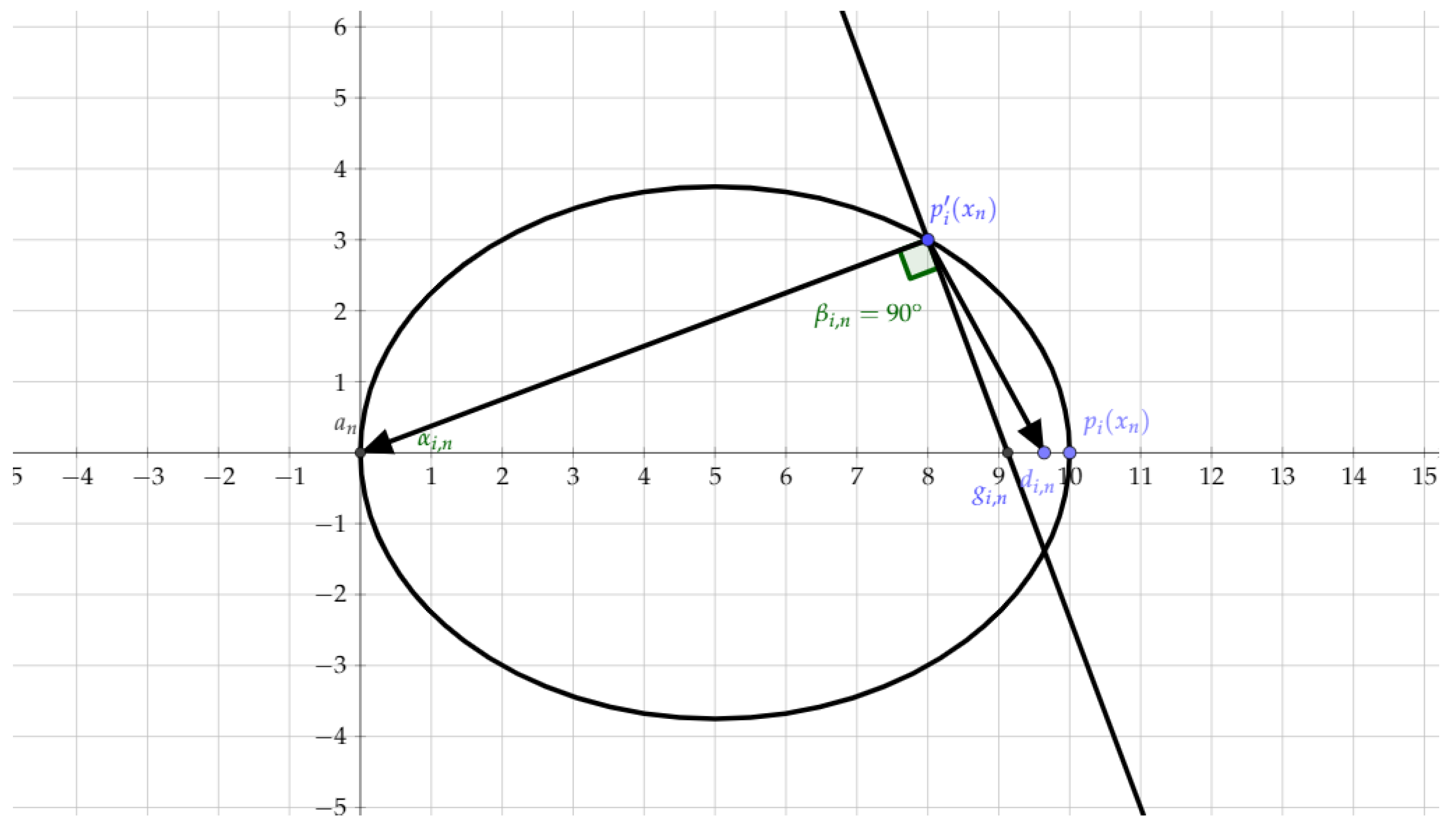
In this section, we show how the results of Section 3 may be used to define a strongly convergent cyclic projection algorithm in the case where the sets $S_i$ are only expandable in convex sets, but not into uniformly convex sets. To our knowledge, this method is new, even in the convex case. The underlying idea of the algorithm is as follows. First, note that the condition ${\mathrm{C}}_4$ is realistic for the type of nonconvex sets considered in this paper, and may be interpreted as a strong consistency condition. On the other hand, in many cases, a trivial sequence ${\left(a_n\right)}_{n\in \mathbb{N}}$ where $a_n\in T_n$ for all n in $\mathbb{N}$ is already known, as in the applications presented in Section 5. Using this sequence, we define a projection method which converges strongly to a point in ${\bigcap }_{i\in I}{S}_i$. For every n in $\mathbb{N}$, i in I, and $a_n$ in $T_n$, $B_{i,n}$ will denote the closed ellipsoid with main axis $[a_n,p_i\left(x_n\right)]$, with center $1/2(a_n+p_i\left(x_n\right))$, which is rotationally invariant around this axis and with maximal radius equal to $|a_n-p_i\left(x_n\right)|/2$ and with minimal radius equal to $\gamma |a_n-p_i\left(x_n\right)|/2$ for some $\gamma \in (0,1)$. We denote by $p_i^{\prime }\left(x_n\right)$ the projection of $x_n$ onto $B_{i,n}$; see Figure 1.

Definition 5.

(Method of Double Projection onto Convex Expandable Sets)

Assume ${\mathrm{C}}_4$ is satisfied. Given a point $x_0$ in $\mathcal{H}$, two real number α and λ in $(0,1]$, a nonnegative integer M, a sequence $\left(I_n\right)$ of subsets of I and a sequence ${\left(a_n\right)}_{n\in \mathbb{N}}$ where $a_n\in T_n$ for all n in $\mathbb{N}$, the projection method onto stepwise generated uniformly convex sets is iteratively defined by

$$(\forall n\in \mathbb{N})\left\{\begin{array}{cc}1.\hfill & (\forall i\in I_n)p_i^{\prime }\left(x_n\right)=p_{B_{i,n}}\left(x_n\right)\hfill \\ 2.\hfill & \left|\begin{array}{c}-If\exists j\in I_{n}suchthat{p}_j^{\prime }\left(x_n\right)\in \bigcap _{i\in I_n}{S}_i\hfill \\ Then\left|\begin{array}{c}-If{I}_n\ne Iset{I}_n=Iandgoto2\hfill \\ -If{I}_n=Iset{\lambda }_n=1,{\alpha }_{j,n}=1andgoto3\hfill \end{array}\right.\hfill \\ -Elsegoto3\hfill \end{array}\right.\hfill \\ 3.\hfill & x_{n+1}=x_n+{\lambda }_n\sum _{i\in I_n}{\alpha }_{i,n}(p_i^{\prime }\left(x_n\right)-x_n)\hfill \end{array}\right.$$

under the conditions ${\mathrm{C}}_1$, ${\mathrm{C}}_2$, and

$$\begin{array}{cc}\hfill {\mathrm{C}}_3^{\prime }.& (\forall n\in \mathbb{N})\lambda \le {\lambda }_n\le {\mu }_{n}where{\mu }_n=\left\{\begin{array}{cc}\frac{{\sum }_{i\in I_n}{\alpha }_{i,n}{|x_n-p_i^{\prime }\left(x_n\right)|}^2}{|x_n-{\sum }_{i\in I_n}{\alpha }_{i,n}{p}_i^{\prime }\left(x_n\right){|}^2}\hfill & if{x}_n\notin {\bigcap }_{i\in I_n}{B}_{i,n}\hfill \\ 1\hfill & if{x}_n\in {\bigcap }_{i\in I_n}{B}_{i,n}.\hfill \end{array}\right.\hfill \end{array}$$

In the remainder of this section, the sequence ${\left(x_n\right)}_{n\in \mathbb{N}}$ is defined by the algorithm of Definition 5. The main result is the following.

Theorem 2.

If the condition ${\mathrm{C}}_5$ is satisfied, and the sequence ${\left(a_n\right)}_{n\in \mathbb{N}}$ introduced in Definition 5 satisfies ${\mathrm{C}}_6$, then the sequence ${\left(x_n\right)}_{n\in \mathbb{N}}$ converges strongly to a point in ${\bigcap }_{i\in I}{S}_i$.

Proof. 

The method introduced in Definition 5 is a general projection algorithm onto specific uniformly convex sets constructed at each iteration. For every n in $\mathbb{N}$ and each i in I, $a_n$ and $p_i^{\prime }\left(x_n\right)$ belong to $B_{i,n}$. Then Lemma 2 and Lemma 3 where $p_i\left(x_n\right)$ and ${\left(z_n\right)}_{n\in \mathbb{N}}$ are respectively replaced with $p_i^{\prime }\left(x_n\right)$ and ${\left(a_n\right)}_{n\in \mathbb{N}}$ hold true. In the same way, taking ${\left(z_n\right)}_{n\in \mathbb{N}}={\left(a_n\right)}_{n\in \mathbb{N}}$ in the proof of Theorem 1, we deduce that the sequence ${\left(x_n\right)}_{n\in \mathbb{N}}$ converges strongly to some point $x^{*}$ in $\mathcal{H}$. Nevertheless, since $p_i\left(x_n\right)$ is replaced with $p_i^{\prime }\left(x_n\right)$, it is still not clear why $x^{*}\in {\bigcap }_{i\in I}{S}_i$. Let us now address this specific point. Fix n in $\mathbb{N}$, i in I, and $a_n$ in $T_n$. According to ${\mathrm{C}}_5$, $a_n$ and $p_i\left(x_n\right)$ belong to a convex set $C_{i,j_n}\subset S_i$, and $p_i\left(x_n\right)$ is also the projection of $x_n$ onto $C_{i,j_n}$. Hence the Kolmogorov criterion (1) gives $\langle p_i\left(x_n\right)-a_n\mid x_n-p_i\left(x_n\right)\rangle \ge 0$. Therefore

$$\langle p_i\left(x_n\right)-a_n\mid x_n-p_i^{\prime }\left(x_n\right)\rangle +\langle p_i\left(x_n\right)-a_n\mid p_i^{\prime }\left(x_n\right)-p_i\left(x_n\right)\rangle \ge 0$$

which implies

$$\begin{array}{c}\hfill \langle p_i\left(x_n\right)-a_n\mid x_n-p_i^{\prime }\left(x_n\right)\rangle \ge \langle p_i\left(x_n\right)-a_n\mid p_i\left(x_n\right)-p_i^{\prime }\left(x_n\right)\rangle .\end{array}$$

(10)

Moreover, since the segment $[a_n,p_i\left(x_n\right)]$ is the main axis of the ellipsoid $B_{i,n}$ and $p_i^{\prime }\left(x_n\right)\in B_{i,n}$, we have $\langle a_n-p_i\left(x_n\right)\mid p_i^{\prime }\left(x_n\right)-p_i\left(x_n\right)\rangle \ge 0$. Combining this with (10), we get

$$0\le \langle p_i\left(x_n\right)-a_n\mid p_i\left(x_n\right)-p_i^{\prime }\left(x_n\right)\rangle \le \langle p_i\left(x_n\right)-a_n\mid x_n-p_i^{\prime }\left(x_n\right)\rangle \le |p_i\left(x_n\right)-a_n\left|\right|x_n-p_i^{\prime }\left(x_n\right)|.$$

We deduce from Lemma 3(iii) where $p_i\left(x_n\right)$ is replaced with $p_i^{\prime }\left(x_n\right)$ that ${lim}_{n\to \infty }|p_i^{\prime }\left(x_n\right)-x_n|=0$. On the other hand, as $p_i\left(x_n\right)$ is the projection of $x_n$ onto $C_{i,j_n}$, and $a_n\in C_{i,j_n}$, we have $|p_i\left(x_n\right)-a_n|\le |x_n-a_n|$. Moreover, following the same steps as in the proof of Lemma 3(i) gives that $\left(\right|x_n-a_n{\left|\right)}_{n\in \mathbb{N}}$ is bounded, from which we deduce that $\left(\right|p_i\left(x_n\right)-a_n{\left|\right)}_{n\in \mathbb{N}}$ is bounded as well. Therefore we deduce from the last inequality that

$$\underset{n\to \infty }{lim}\langle a_n-p_i\left(x_n\right)\mid p_i^{\prime }\left(x_n\right)-p_i\left(x_n\right)\rangle =0.$$

(11)

Let $x=a_n-p_i\left(x_n\right)$ and $y=p_i^{\prime }\left(x_n\right)-p_i\left(x_n\right)$. Then, we have

$$x-y=a_n-p_i^{\prime }\left(x_n\right)$$

and

$$x-\omega y=\omega \left(\frac{1}{\omega }(a_n+(\omega -1)p_i\left(x_n\right))-p_i^{\prime }\left(x_n\right)\right)$$

(12)

for all $\omega \in \mathbb{R}$.

Assume that $p_i^{\prime }\left(x_n\right)\ne p_i\left(x_n\right)$. Using Claim 1, we get that

$$〈a_n-p_i^{\prime }\left(x_n\right)\mid \frac{1}{{\omega }_{i,n}}(a_n+({\omega }_{i,n}-1)p_i\left(x_n\right))-p_i^{\prime }\left(x_n\right)〉\le 0$$

as long as we enforce

$${\omega }_{i,n}\ge \frac{\langle p_i^{\prime }\left(x_n\right)-a_n\mid p_i\left(x_n\right)-a_n\rangle }{\langle p_i^{\prime }\left(x_n\right)-a_n\mid p_i\left(x_n\right)-p_i^{\prime }\left(x_n\right)\rangle }.$$

(13)

In particular, we can take

$${\omega }_{i,n}=max\left\{\frac{\langle p_i^{\prime }\left(x_n\right)-a_n\mid p_i\left(x_n\right)-a_n\rangle }{\langle p_i^{\prime }\left(x_n\right)-a_n\mid p_i\left(x_n\right)-p_i^{\prime }\left(x_n\right)\rangle },ϵ\right\}$$

(14)

for any appropriately chosen $ϵ>0$. Using Niculescu’s Lemma 4 in Appendix B, we obtain that

$$\left(\sqrt{\frac{1}{{\omega }_{i,n}}}+\sqrt{\frac{{\omega }_{i,n}}{1}}\right)\frac{\langle a_n-p_i\left(x_n\right),p_i^{\prime }\left(x_n\right)-p_i\left(x_n\right)\rangle }{2|a_n-p_i\left(x_n\right)|}\ge |p_i^{\prime }\left(x_n\right)-p_i\left(x_n\right)|.$$

(15)

Note that this inequality also holds without resorting to Claim 1 if $p_i^{\prime }\left(x_n\right)=p_i\left(x_n\right)$. According to Theorem 1, ${\left(x_n\right)}_{n\in \mathbb{N}}$ and ${\left(p_i^{\prime }\left(x_n\right)\right)}_{n\in \mathbb{N}}$ are strongly convergent to a point $x^{*}$ in $\mathcal{H}$. We now split the remainder of the argument into the following complementary cases involving an increasing function $\sigma$: $\mathbb{N}\mapsto \mathbb{N}$ which parametrises possible subsequences.

• If the sequence $\left(\right|a_n-p_i^{\prime }\left(x_n\right){\left|\right)}_{n\in \mathbb{N}}$ converges to zero, then using Claim 2, $\left(\right|p_i^{\prime }\left(x_n\right)-p_i\left(x_n\right){\left|\right)}_{n\in \mathbb{N}}$ also converges to zero. Therefore, ${\left(p_i\left(x_n\right)\right)}_{n\in \mathbb{N}}$ is also strongly convergent to $x^{*}$ for each i in I. Since each set $S_i$ is closed, we again conclude that $x^{*}\in {\bigcap }_{i\in I}{S}_i$.
• If the sequence $\left(\right|a_n-p_i^{\prime }\left(x_n\right){\left|\right)}_{n\in \mathbb{N}}$ does not converge to zero, and the sequence ${\left(\langle p_i^{\prime }\left(x_n\right)-a_n\mid p_i\left(x_n\right)-p_i^{\prime }\left(x_n\right)\rangle \right)}_{n\in \mathbb{N}}$ converges to zero, then we must have $|a_{\sigma \left(n\right)}-p_i^{\prime }\left(x_{\sigma \left(n\right)}\right)|>ϵ$ for some $ϵ>0$ and some subsequence indexed by an appropriately chosen increasing function $\sigma$. This implies in particular that

  $$\underset{n\to +\infty }{lim}|p_i\left(x_{\sigma \left(n\right)}\right)-p_i^{\prime }\left(x_{\sigma \left(n\right)}\right)\left|\right|cos\left(p_i^{\prime }\left(x_{\sigma \left(n\right)}\right)-a_{\sigma \left(n\right)},p_i\left(x_{\sigma \left(n\right)}\right)-p_i^{\prime }\left(x_{\sigma \left(n\right)}\right)\right)|=0.$$
  As a result, either

  $$\underset{n\to +\infty }{lim}cos\left(p_i^{\prime }\left(x_{\sigma \left(n\right)}\right)-a_{\sigma \left(n\right)},p_i\left(x_{\sigma \left(n\right)}\right)-p_i^{\prime }\left(x_{\sigma \left(n\right)}\right)\right)=0$$

  (16)

  or

  $$\underset{n\to +\infty }{lim}|p_i\left(x_{\sigma \left(n\right)}\right)-p_i^{\prime }\left(x_{\sigma \left(n\right)}\right)|=0.$$
  Notice further that (16) holds only if $\left(\right|p_i\left(x_{\sigma \left(n\right)}\right)-p_i^{\prime }\left(x_{\sigma \left(n\right)}\right){\left|\right)}_{n\in \mathbb{N}}$ converges to zero. Thus, both cases simplify into the conclusion that $\left(\right|p_i\left(x_{\sigma \left(n\right)}\right)-p_i^{\prime }\left(x_{\sigma \left(n\right)}\right){\left|\right)}_{n\in \mathbb{N}}$ converges to zero. Therefore ${\left(p_i\left(x_{\sigma \left(n\right)}\right)\right)}_{n\in \mathbb{N}}$ is also strongly convergent to $x^{*}$ for each i in I. Since each set $S_i$ is closed, we again conclude that $x^{*}\in {\bigcap }_{i\in I}{S}_i$.
• If both sequences $\left(\right|a_n-p_i^{\prime }\left(x_n\right){\left|\right)}_{n\in \mathbb{N}}$ and ${\left(\langle p_i^{\prime }\left(x_n\right)-a_n\mid p_i\left(x_n\right)-p_i^{\prime }\left(x_n\right)\rangle \right)}_{n\in \mathbb{N}}$ do not converge to zero, then $|a_{\sigma \left(n\right)}-p_i^{\prime }\left(x_{\sigma \left(n\right)}\right)|>ϵ$ and $\langle p_i^{\prime }\left(x_{\sigma \left(n\right)}\right)-a_{\sigma \left(n\right)}\mid p_i\left(x_{\sigma \left(n\right)}\right)-p_i^{\prime }(x_{\sigma \left(n\right)}\rangle >ϵ$ for some $ϵ>0$ and for some subsequence indexed by an appropriately chosen increasing function $\sigma$. Since $|a_n-p_i\left(x_n\right)|$ is the length of the main axis of $B_{i,n}$, and, as such, bounds from above the distance between any two points in $B_{i,n}$, we deduce that $|a_n-p_i^{\prime }\left(x_n\right)|\le |a_n-p_i\left(x_n\right)|$. Furthermore, since the sequences $\left(\right|a_n-p_i\left(x_n\right){\left|\right)}_{n\in \mathbb{N}}$ and $\left(\right|a_n-x_n{\left|\right)}_{n\in \mathbb{N}}$ are bounded, we deduce that

  $$|a_n-p_i\left(x_n\right)|\le |a_n-x_n|\le B$$

  for some $B>0$. Then using the Cauchy-Schwarz inequality in the numerator in (14), we get

  $${\omega }_{i,\sigma \left(n\right)}\in [ϵ,\frac{B^2}{ϵ}]$$

  for some $ϵ\in (0,B)$. Since $|a_{\sigma \left(n\right)}-p_i\left(x_{\sigma \left(n\right)}\right)|>ϵ$, we deduce from (11) and (15) that $\left(\right|p_i^{\prime }\left(x_{\sigma \left(n\right)}\right)-p_i\left(x_{\sigma \left(n\right)}\right){\left|\right)}_{n\in \mathbb{N}}$ converges to zero. Therefore, ${\left(p_i\left(x_{\sigma \left(n\right)}\right)\right)}_{n\in \mathbb{N}}$ is also strongly convergent to $x^{*}$ for each i in I. Since each set $S_i$ is closed, we again conclude that $x^{*}\in {\bigcap }_{i\in I}{S}_i$.

These previous cases cover all the possible cases and all lead to the conclusion that $x^{*}\in {\bigcap }_{i\in I}{S}_i$. The proof is thus complete. ☐

The two following claims were instrumental in the proof of Theorem 2. We now provide their proofs.

Claim 1.

Assume that $p_i^{\prime }\left(x_n\right)\ne p_i\left(x_n\right)$. Then

$$\begin{array}{c}\hfill \frac{\langle p_i^{\prime }\left(x_n\right)-a_n\mid p_i\left(x_n\right)-a_n\rangle }{\langle p_i^{\prime }\left(x_n\right)-a_n\mid p_i\left(x_n\right)-p_i^{\prime }\left(x_n\right)\rangle }\end{array}$$

(17)

is a well defined nonnegative real number. Moreover, we have

$$〈a_n-p_i^{\prime }\left(x_n\right)\mid \frac{1}{{\omega }_{i,n}}(a_n+({\omega }_{i,n}-1)p_i\left(x_n\right))-p_i^{\prime }\left(x_n\right)〉\le 0$$

(18)

for all

$${\omega }_{i,n}\ge \frac{\langle p_i^{\prime }\left(x_n\right)-a_n\mid p_i\left(x_n\right)-a_n\rangle }{\langle p_i^{\prime }\left(x_n\right)-a_n\mid p_i\left(x_n\right)-p_i^{\prime }\left(x_n\right)\rangle }.$$

Proof. 

We have $p_i^{\prime }\left(x_n\right)\notin [a_n,p_i\left(x_n\right)]$. Indeed, assume for contradiction that $p_i^{\prime }\left(x_n\right)\in [a_n,p_i\left(x_n\right)]$. This would imply that $p_i^{\prime }\left(x_n\right)$ lies in the interior of $B_{i,n}$ and therefore $x_n=p_i^{\prime }\left(x_n\right)$. However, since by convexity of $C_{i,j_n}$, $[a_n,p_i\left(x_n\right)]\subset C_{i,j_n}$, this would imply that $x_n\in C_{i,j_n}$, and therefore $p_i^{\prime }\left(x_n\right)=x_n=p_i\left(x_n\right)$, the sought-after contradiction.

Consider now the 2D plane containing $a_n$, $p_i\left(x_n\right)$ and $p_i^{\prime }\left(x_n\right)$. Set $g_n$ to be at the intersection of the line perpendicular at $p_i^{\prime }\left(x_n\right)$ to $[a_n,p_i^{\prime }\left(x_n\right)]$ with the segment $[a_n,p_i\left(x_n\right)]$ (see Figure 1). First, we have

$$\langle p_i^{\prime }\left(x_n\right)-a_n\mid p_i\left(x_n\right)-a_n\rangle =cos\left({\alpha }_{i,n}\right)|p_i^{\prime }\left(x_n\right)-a_n\left|\right|p_i\left(x_n\right)-a_n|$$

and

$$|p_i^{\prime }\left(x_n\right)-a_n{|}^2=\langle g_n-a_n\mid p_i^{\prime }\left(x_n\right)-a_n\rangle =cos\left({\alpha }_{i,n}\right)|g_n-a_n\left|\right|p_i^{\prime }\left(x_n\right)-a_n|$$

from which we obtain

$$|g_n-a_n|=\frac{|p_i^{\prime }\left(x_n\right)-a_n{|}^2|p_i\left(x_n\right)-a_n|}{\langle p_i^{\prime }\left(x_n\right)-a_n\mid p_i\left(x_n\right)-a_n\rangle }$$

(19)

Since $B_{i,n}$ is an ellipse with maximal axis $[a_n,p_i\left(x_n\right)]$, our next step is to express $g_n$ as the convex combination

$$g_n={\theta }_{i,n}{a}_n+(1-{\theta }_{i,n})p_i\left(x_n\right)$$

(20)

of $a_n$ and $p_i\left(x_n\right)$ for some ${\theta }_{i,n}\in [0,1]$. Notice that (20) implies

$$|g_n-a_n|=(1-{\theta }_{i,n})|p_i\left(x_n\right)-a_n|,$$

which itself gives

$${\theta }_{i,n}=1-\frac{|g_n-a_n|}{|p_i\left(x_n\right)-a_n|}.$$

Using (19), we get

$${\theta }_{i,n}=1-\frac{|p_i^{\prime }\left(x_n\right)-a_n{|}^2}{\langle p_i^{\prime }\left(x_n\right)-a_n\mid p_i\left(x_n\right)-a_n\rangle }=\frac{\langle p_i^{\prime }\left(x_n\right)-a_n\mid p_i\left(x_n\right)-p_i^{\prime }\left(x_n\right)\rangle }{\langle p_i^{\prime }\left(x_n\right)-a_n\mid p_i\left(x_n\right)-a_n\rangle }.$$

Notice further that, by construction, since $[a_n,p_i\left(x_n\right)]$ is the main axis of $B_{i,n}$ and since, by assumption, $p_i^{\prime }\left(x_n\right)\ne p_i\left(x_n\right)$, we have (see Figure 1)

$$\begin{array}{cc}\hfill \langle p_i^{\prime }\left(x_n\right)-a_n\mid p_i\left(x_n\right)-p_i^{\prime }\left(x_n\right)\rangle & >0.\hfill \end{array}$$

(21)

Then, setting

$$d_n=\frac{1}{{\omega }_{i,n}}(a_n+({\omega }_{i,n}-1)p_i\left(x_n\right))$$

we see that we need to take ${\omega }_{i,n}\ge 1/{\theta }_{i,n}$, i.e.,

$${\omega }_{i,n}\ge \frac{\langle p_i^{\prime }\left(x_n\right)-a_n\mid p_i\left(x_n\right)-a_n\rangle }{\langle p_i^{\prime }\left(x_n\right)-a_n\mid p_i\left(x_n\right)-p_i^{\prime }\left(x_n\right)\rangle },$$

(which, owing to (21), is well defined), in order to ensure that

$$〈a_n-p_i^{\prime }\left(x_n\right)\mid d_n-p_i^{\prime }\left(x_n\right)〉\le 0$$

i.e., (18) holds. Finally, (19) and (21) together ensure that (17) is nonnegative. ☐

Claim 2.

We have

$$|a_n-p_i^{\prime }\left(x_n\right)|\ge |p_i^{\prime }\left(x_n\right)-p_i\left(x_n\right)|.$$

Proof. 

By definition of $p_i\left(x_n\right)$, the fact that $a_n\in S_i$ implies that

$$|p_i\left(x_n\right)-x_n|\le |a_n-x_n|.$$

Thus $x_n$ belongs to the half space

$$H=\left\{x\in \mathcal{H};\langle x-\frac{1}{2}(a_n+p_i\left(x_n\right))\mid p_i\left(x_n\right)-\frac{1}{2}(a_n+p_i\left(x_n\right))\rangle \ge 0\right\}$$

which is the set of points in $\mathcal{H}$ which are closer to $p_i\left(x_n\right)$ than $a_n$. Clearly, $p_i^{\prime }\left(x_n\right)\in H$ as well, which completes the proof. ☐

5. Applications

5.1. MRI Image Reconstruction: The Infinite-Dimensional Hilbert Space Setting

The field of inverse problems was extensively investigated in the last five decades, fueled in particular by the many challenged in medical imaging. Projection methods have played an important role in the development of efficient reconstruction techniques [25], a well studied example being the method of projection onto convex sets (POCS) [2]. In recent years, techniques from penalised estimation have gained increasing popularity since the discovery of the compressed sensing paradigm, allowing for fewer measurements to be collected whilst achieving remarkable reconstruction performance. One penalisation approach which has been a center of focus since its introduction is the Rudin Osher Fatemi functional [26], which can be described as follows: the reconstructed image u is the solution of the minimization problem,

$$\underset{u\in BV(\Omega )}{argmin}{\parallel u\parallel }_{\mathrm{TV}(\Omega )}+\frac{\lambda }{2}{\int }_{\Omega }{(y_{obs}\left(x\right)-\mathcal{A}\left[u\right]\left(x\right))}^{2}dx$$

where $\lambda$ is a positive relaxation parameter and the term ${\parallel u\parallel }_{\mathrm{TV}(\Omega )}$ is defined in Appendix A. The term ${\int }_{\Omega }{(y_{obs}\left(x\right)-\mathcal{A}\left[u\right]\left(x\right))}^{2}dx$ is called the fidelity term and the term ${\parallel u\parallel }_{\mathrm{TV}(\Omega )}$ is called the regularisation term. This infinite-dimensional minimization problem enforces the solution, which is a priori in $L^2(\Omega )$, to satisfy a finite bounded variation (BV) norm constraint.

One important remark is that the optimisation problem can be turned into a pure feasibility problem by imposing the $TV$-norm and the fidelity terms to be less than or equal to a certain tolerance. Using this approach, one can define an alternating projection procedure as in Algorithm 1 below, where we will use the forward operator $\mathcal{A}={\mathcal{F}}_{partial}$, the partial Fourier Transform which plays a central role in MRI. The usual Fourier transform will be denoted by $\mathcal{F}$ as usual.

In this example, we will use the projections on the sets

$$\begin{array}{cc}\hfill S_1& =\left\{u\in L^2(\Omega )\mid {\int }_{\Omega }{(\lambda y_{obs}-\mathcal{A}\left[u\right]\left(x\right))}^{2}dx\le \lambda {\eta }_{fid},\lambda \in {\mathbb{R}}_{+}\right\},\hfill \end{array}$$

$$\begin{array}{cc}\hfill S_2& =\left\{u\in L^2(\Omega )\mid {\parallel u\parallel }_{p,\mathrm{TV}(\Omega )}\le {\eta }_{TV}\right\},\hfill \end{array}$$

$$\begin{array}{cc}\hfill S_3& =\left\{u\in L^2(\Omega )\mid {\mathcal{F}}_{partial}\left[u\right]=\lambda y_{obs},\lambda \in {\mathbb{R}}_{+}\right\}.\hfill \end{array}$$

The set $S_2$ is not convex for $p\in (0,1)$, but, since the epigraph of ${|·|}_{p,TV(\Omega )}$ is a cone, the set $S_2$ is expandable into convex sets as discussed in [22,23]. Notice that when the scaling factor $\lambda$ is dropped in the definition of $S_1$ and $S_3$, the problem is equivalent to the standard $TV$-penalised reconstruction approach. Introducing this scaling factor allows to recover a solution up to a scaling, which can easily be recovered by rescaling the solution by using the constraint ${\mathcal{F}}_{partial}\left[u\right]=y_{obs}$ as a post-processing step. The introduction of the scaling $\alpha$ in these definition allows the null function to belong to the intersection of the sets $S_1$, $S_2$ and $S_3$. Thus, we will set $a_n=0$, $n\in \mathbb{N}$ in the sequel. In what follows, ${\tilde{y}}_{obs}$ will be the function will value equal to zero except for the observed frequencies which are taken as the observed values.

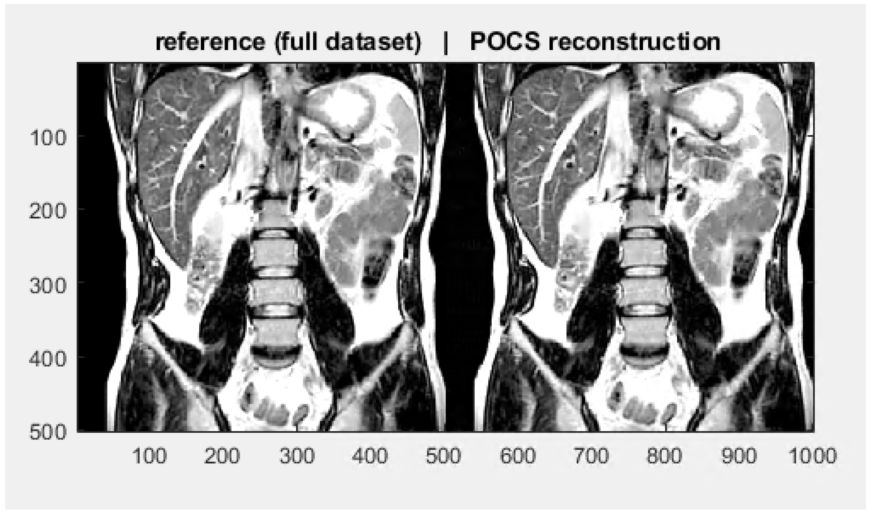
Our implementation is described in Algorithm 1. Experiments were made after incorporating the projection onto the $TV$ ball into a freely available code provided in [27]. The fidelity term was set to ${\eta }_{fid}={10}^{-3}$ and the regularisation term ${\eta }_{TV}$ was tuned using cross validation. The projection onto the $TV$-ball was computed using the method described in [28]. In order to avoid numerical instabilities, the iterates were rescaled every 10 iteration, which does not change the convergence analysis due to conic invariance of our formulation. We chose very thin ellipsoids $B_{i,n}$ by setting $\alpha ={10}^{-6}$. A numerical illustration is given in Figure 2 below. Extensive numerical simulations will be presented in a forthcoming paper devoted to a thorough study of projection methods for MRI and X-ray computed tomography (XCT).

Algorithm 1: Alternating projection method for MRI for $p=1$.

Since $S_1$ and $S_3$ are convex and $S_2$ is expandable into convex sets, we deduce from Theorem 2 that Algorithm 1 converges strongly to a point in ${\bigcap }_{i=1}^3{S}_i$.

5.2. A Uniformly Convex Version of Cadzow’s Method

The method presented in Section 4 is now applied to a denoising problem in the spirit of Cadzow’s method [16].

Let $x={[x_0,\dots ,x_{N-1}]}^{\top }$ be a complex-valued vector of length N. Let $\mathcal{H}$ be a linear operator which maps x into the set of Hankel $L\times K$ matrices, with $L\ge K$, $L+K=N+1$, defined by setting the $(i,j)$ component to the value $x_{i+j-2}$ i.e.,

$$\mathcal{H}\left(x\right)=\left[\begin{array}{ccccc}{x}_0& x_1& x_2& \cdots & x_{K-1}\\ x_1& x_2& x_3& \cdots & x_K\\ x_2& x_3& x_4& \cdots & x_{K+1}\\ ⋮& ⋮& ⋮& ⋮& ⋮\\ x_{L-1}& x_L& x_{L+1}& \cdots & x_{N-1}\end{array}\right].$$

The adjoint operator associated with $\mathcal{H}$, denoted by ${\mathcal{H}}^{*}$, is a linear map from $L\times K$ matrices to vectors of length N, obtained by averaging each skew-diagonal.

The denoising problem we consider in this section is the one of estimating a signal x corrupted by random noise, as described in the observation model

$$\begin{array}{cc}\hfill y_t& =x_t+{ϵ}_t,\hfill \end{array}$$

for $t=0,\dots ,N-1$, where

• $x_t$ is a sum of damped exponential components, i.e.,

  $$x_t=\sum _{k=-\kappa }^{\kappa }{c}_k{\rho }_k^{t}exp\left(2\iota \pi f_{k}t\right),$$

  with $2\kappa +1\le K$, ${\rho }_k$ a real damping factor satisfying $|{\rho }_k|\le 1$, $f_k$ a real number representing a frequency and $c_k$ a complex coefficient,
• ${ϵ}_t$ is a random noise.

This denoising problem is of crucial importance in many applications and is also known as super-resolution in the literature; see [16,29,30,31,32,33]. The main motivation behind Cadzow’s algorithm is that many signals of interest have low rank Hankelization. In mathematical terms, we can often look for approximations and denoising, for signals which satisfy the constraint that rank($\mathcal{H}\left(x\right))=r$ where $r\le 2\kappa +1$. Such constraints are important when the observed signal is corrupted with additive noise, which increases the rank of $\mathcal{H}\left(x\right)$. Consequently, an intuitive way of estimating x from y is to do rank reduction: starting from $x^{\left(0\right)}=y={[y_0,\dots ,y_{N-1}]}^{\top }$, the Cadzow’s algorithm iteratively updates the estimate via the following rule

$$x^{(n+1)}={\mathcal{H}}^{*}({\mathcal{T}}_r(\mathcal{H}(x^{(n)}))),n=0,1,\dots$$

Here ${\mathcal{T}}_r$ computes the truncated singular value decomposition (SVD) of any $L\times K$ matrix X, that is,

$${\mathcal{T}}_r\left(X\right)=\sum _{j=1}^r{\sigma }_j{u}_j{v}_j^{*},$$

with

$$\begin{array}{cc}\hfill X& =\sum _{j=1}^K{\sigma }_j{u}_j{v}_j^{*}\hfill \end{array}$$

being an SVD of X and with ${\sigma }_1\ge {\sigma }_2\ge \dots \ge {\sigma }_K$ being the singular values. As is now well known, Cadzow’s algorithm is easily interpreted as a method of alternating projections in the matrix domain [23]. Denote by ${\mathcal{P}}_{{\mathcal{M}}_r}$ the projection onto the set ${\mathcal{M}}_r$ of $L\times K$ matrices of rank r, and by ${\mathcal{P}}_{{\mathcal{M}}_H}$ the projection onto the space ${\mathcal{M}}_H$ of $L\times K$ Hankel matrices. Then, Cadzow’s method is easily seen to be equivalent to the following matrix recursions

$$X^{(n+1)}={\mathcal{P}}_{{\mathcal{M}}_H}\left({\mathcal{P}}_{{\mathcal{M}}_r}\left(X^{\left(n\right)}\right)\right),n=0,1,\dots$$

Since ${\mathcal{M}}_H$ is convex and ${\mathcal{M}}_r$ is expandable into convex sets, we deduce from the main result of [22] that Cadzow’s method has cluster points in ${\mathcal{M}}_H\cap {\mathcal{M}}_r$. On the other hand, applying the method of Section 4 can be advantageous in the application of projection methods to the case of low rank matrix constraints such as in the application of Cadzow’s method. In particular, our method shows that the SVD can be computed only approximately in the first iterations and still belong to the ellipsoids $B_{i,n}$, thus implying possibly important computational savings. Our new method converges to a point in ${\mathcal{M}}_H\cap {\mathcal{M}}_r$.

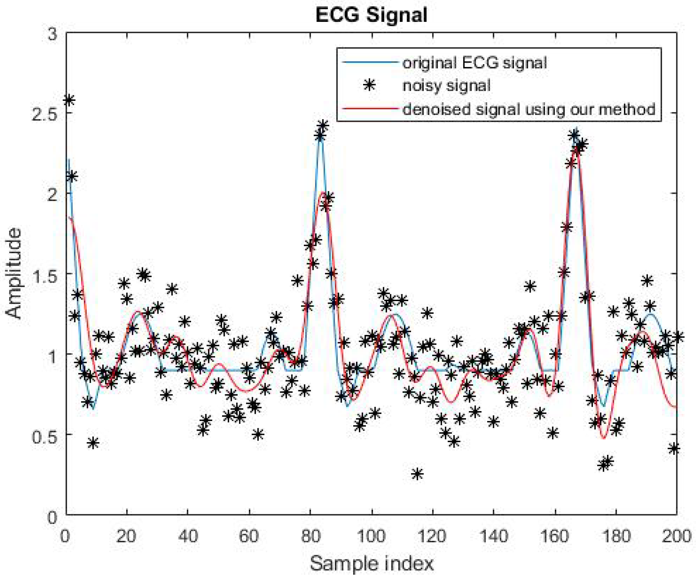
An example showing the efficiency of Cadzow’s method is presented in Figure 3 below. In this experiment, we set the signal-to-noise ratio (SNR) to 3.5 dB and the rank constraint equal to 15 (an appropriate choice for the rank can be made using statistical techniques such as cross-validation). We took $K=\lfloor N/2-10\rfloor$.

6. Conclusions and Future Work

The work presented in this paper is a follow on project to the work of [22]. We obtain strong convergence results in Hilbert spaces in the case of uniformly convex expandable sets, a notion which refines the definition of convex expandable sets introduced in [22,23]. We showed that the proposed methods apply to practical inverse and denoising problems which are instrumental in engineering and signal and data analytics.

Future work is planned in developing new and faster algorithms for nonconvex feasibility problems, using acceleration schemes such as Richardon’s extrapolation [34].

References

- Bauschke, H.H.; Combettes, P.L. Convex Analysis and Monotone Operator Theory in Hilbert Spaces; Springer: Berlin/Heidelberg, Germany, 2011; Volume 408. [Google Scholar]
- Escalante, R.; Raydan, M. Alternating Projection Methods; SIAM: Philadelphia, PA, USA, 2011. [Google Scholar]
- Gurin, L.; Polyak, B.T.; Raik, È.V. The method of projections for finding the common point of convex sets. Zhurnal Vychislitel’noi Matematiki i Matematicheskoi Fiziki 1967, 7, 1211–1228. [Google Scholar]
- Ottavy, N. Strong convergence of projection-like methods in Hilbert spaces. J. Optim. Theory Appl. 1988, 56, 433–461. [Google Scholar] [CrossRef]
- Combettes, P.L.; Puh, H. Iterations of parallel convex projections in Hilbert spaces. Numer. Funct. Anal. Optim. 1994, 15, 225–243. [Google Scholar] [CrossRef]
- Grigoriadis, K.M. Optimal H∞ model reduction via linear matrix inequalities: Continuous-and discrete-time cases. Syst. Control Lett. 1995, 26, 321–333. [Google Scholar] [CrossRef]
- Babazadeh, M.; Nobakhti, A. Direct Synthesis of Fixed-Order H∞ Controllers. IEEE Trans. Autom. Control 2015, 60, 2704–2709. [Google Scholar] [CrossRef]
- Li, Z.; Dai, Y.H.; Gao, H. Alternating projection method for a class of tensor equations. J. Comput. Appl. Math. 2019, 346, 490–504. [Google Scholar] [CrossRef]
- Combettes, P. The convex feasibility problem in image recovery. In Advances in Imaging and Electron Physics; Elsevier: Amsterdam, The Netherlands, 1996; Volume 95, pp. 155–270. [Google Scholar]
- Krol, A.; Li, S.; Shen, L.; Xu, Y. Preconditioned alternating projection algorithms for maximum a posteriori ECT reconstruction. Inverse Probl. 2012, 28, 115005. [Google Scholar] [CrossRef] [Green Version]
- Herman, G.T. Fundamentals of Computerized Tomography: Image Reconstruction From Projections; Springer Science & Business Media: Berlin/Heidelberg, Germany, 2009. [Google Scholar]
- McGibney, G.; Smith, M.; Nichols, S.; Crawley, A. Quantitative evaluation of several partial Fourier reconstruction algorithms used in MRI. Magn. Reson. Med. 1993, 30, 51–59. [Google Scholar] [CrossRef]
- Ticozzi, F.; Zuccato, L.; Johnson, P.D.; Viola, L. Alternating projections methods for discrete-time stabilization of quantum states. IEEE Trans. Autom. Control 2017, 63, 819–826. [Google Scholar] [CrossRef]
- Drusvyatskiy, D.; Li, C.K.; Pelejo, D.C.; Voronin, Y.L.; Wolkowicz, H. Projection methods for quantum channel construction. Quantum Inf. Process. 2015, 14, 3075–3096. [Google Scholar] [CrossRef]
- Grigoriadis, K.M.; Beran, E.B. Alternating projection algorithms for linear matrix inequalities problems with rank constraints. In Advances in Linear Matrix Inequality Methods in Control; SIAM: Philadelphia, PA, USA, 2000; pp. 251–267. [Google Scholar]
- Cadzow, J.A. Signal enhancement-a composite property mapping algorithm. IEEE Trans. Acoust. Speech Signal Process. 1988, 36, 49–62. [Google Scholar] [CrossRef] [Green Version]
- Bauschke, H.H.; Combettes, P.L.; Luke, D.R. Phase retrieval, error reduction algorithm, and Fienup variants: A view from convex optimization. J. Opt. Soc. Am. A 2002, 19, 1334–1345. [Google Scholar] [CrossRef] [PubMed] [Green Version]
- Chu, M.T.; Funderlic, R.E.; Plemmons, R.J. Structured low rank approximation. Linear Algebra Its Appl. 2003, 366, 157–172. [Google Scholar] [CrossRef] [Green Version]
- Markovsky, I.; Usevich, K. Structured low-rank approximation with missing data. SIAM J. Matrix Anal. Appl. 2013, 34, 814–830. [Google Scholar] [CrossRef] [Green Version]
- Elser, V. Learning Without Loss. arXiv 2019, arXiv:1911.00493. [Google Scholar]
- Combettes, P.L.; Trussell, H.J. Method of successive projections for finding a common point of sets in metric spaces. J. Optim. Theory Appl. 1990, 67, 487–507. [Google Scholar] [CrossRef]
- Chretien, S.; Bondon, P. Cyclic projection methods on a class of nonconvex sets. Numer. Funct. Anal. Optim. 1996, 17, 37–56. [Google Scholar]
- Chrétien, S. Methodes de projection pour L’optimisation ensembliste non convexe. Ph.D. Thesis, Sciences Po, Paris, France, 1996. [Google Scholar]
- Bauschke, H.H.; Borwein, J.M. On projection algorithms for solving convex feasibility problems. SIAM Rev. 1996, 38, 367–426. [Google Scholar] [CrossRef] [Green Version]
- Censor, Y.; Chen, W.; Combettes, P.L.; Davidi, R.; Herman, G.T. On the effectiveness of projection methods for convex feasibility problems with linear inequality constraints. Comput. Optim. Appl. 2012, 51, 1065–1088. [Google Scholar] [CrossRef]
- Rudin, L.I.; Osher, S.; Fatemi, E. Nonlinear total variation based noise removal algorithms. Phys. D Nonlinear Phenom. 1992, 60, 259–268. [Google Scholar] [CrossRef]
- Michael, V. MRI Partial Fourier Reconstruction with POCS. Available online: https://fr.mathworks.com/matlabcentral/fileexchange/39350-mri-partial-fourier-reconstruction-with-pocs?s_tid=prof_contriblnk (accessed on 13 February 2020).
- Condat, L. Discrete total variation: New definition and minimization. SIAM J. Imaging Sci. 2017, 10, 1258–1290. [Google Scholar] [CrossRef] [Green Version]
- Plonka, G.; Potts, D.; Steidl, G.; Tasche, M. Numerical Fourier Analysis: Theory and Applications; Book Manuscript; Springer: Berlin/Heidelberg, Germany, 2018. [Google Scholar]
- Al Sarray, B.; Chrétien, S.; Clarkson, P.; Cottez, G. Enhancing Prony’s method by nuclear norm penalization and extension to missing data. Signal Image Video Process. 2017, 11, 1089–1096. [Google Scholar] [CrossRef]
- Barton, E.; Al-Sarray, B.; Chrétien, S.; Jagan, K. Decomposition of Dynamical Signals into Jumps, Oscillatory Patterns, and Possible Outliers. Mathematics 2018, 6, 124. [Google Scholar] [CrossRef] [Green Version]
- Moitra, A. Super-resolution, extremal functions and the condition number of Vandermonde matrices. In Proceedings of the Forty-Seventh Annual ACM Symposium on Theory Of Computing, Chicago, IL, USA, 22–26 June 2015; pp. 821–830. [Google Scholar]
- Chrétien, S.; Tyagi, H. Multi-kernel unmixing and super-resolution using the Modified Matrix Pencil method. J. Fourier Anal. Appl. 2020, 26, 18. [Google Scholar] [CrossRef] [Green Version]
- Bach, F. On the Unreasonable Effectiveness of Richardson Extrapolation. Available online: https://francisbach.com/richardson-extrapolation/ (accessed on 13 February 2020).
- Dragomir, S.S. A generalisation of the Cassels and Greub-Reinboldt inequalities in inner product spaces. arXiv 2003, arXiv:math/0306352. [Google Scholar]
- Niculescu, C.P. Converses of the Cauchy-Schwartz Inequality in the C*-Framework. RGMIA Research Report Collection. 2001, Volume 4. Available online: https://rgmia.org/v4n1.php (accessed on 15 February 2020).
Figure 1.
Section of the ellipsoid .
Figure 2.
POCS reconstruction with 30 iterations.
Figure 3.
Application of our method to denoising a benchmark Electrocardiogram (ECG) type signal.
© 2020 by the authors. Licensee MDPI, Basel, Switzerland. This article is an open access article distributed under the terms and conditions of the Creative Commons Attribution (CC BY) license (http://creativecommons.org/licenses/by/4.0/).
Share and Cite
MDPI and ACS Style
Chrétien, S.; Bondon, P. Projection Methods for Uniformly Convex Expandable Sets. Mathematics 2020, 8, 1108. https://doi.org/10.3390/math8071108
AMA Style
Chrétien S, Bondon P. Projection Methods for Uniformly Convex Expandable Sets. Mathematics. 2020; 8(7):1108. https://doi.org/10.3390/math8071108
Chicago/Turabian StyleChrétien, Stéphane, and Pascal Bondon. 2020. "Projection Methods for Uniformly Convex Expandable Sets" Mathematics 8, no. 7: 1108. https://doi.org/10.3390/math8071108
Note that from the first issue of 2016, this journal uses article numbers instead of page numbers. See further details here.