When Inaccuracies in Value Functions Do Not Propagate on Optima and Equilibria

Abstract

We study general classes of discrete time dynamic optimization problems and dynamic games with feedback controls. In such problems, the solution is usually found by using the Bellman or Hamilton–Jacobi–Bellman equation for the value function in the case of dynamic optimization and a set of such coupled equations for dynamic games, which is not always possible accurately. We derive general rules stating what kind of errors in the calculation or computation of the value function do not result in errors in calculation or computation of an optimal control or a Nash equilibrium along the corresponding trajectory. This general result concerns not only errors resulting from using numerical methods but also errors resulting from some preliminary assumptions related to replacing the actual value functions by some a priori assumed constraints for them on certain subsets. We illustrate the results by a motivating example of the Fish Wars, with singularities in payoffs.

1. Introduction

Finding an optimal control in the feedback form or a feedback Nash equilibrium in a dynamic game is complicated, especially if the analytic solution cannot be found. The appropriate methods, based on the Bellman equation or a set of coupled Bellman equations, respectively, require finding the value function on the whole state space or at least a large invariant subset of it (for the principle of optimality, i.e., necessity of the Bellman equation in the infinite horizon see e.g., Stokey, Lucas and Prescott [1], Kamihigashi [2], Wiszniewska-Matyszkiel and Singh [3]) with appropriate terminal condition (for the infinite horizon, necessity has been proven in Wiszniewska-Matyszkiel and Singh [3]).

Currently, the substantial focus in research by mathematicians is on high accuracy of the solution of the Bellman equation or the set of Bellman equations in the case of numerical solutions, as well as the existence and uniqueness in some classes of functions or methods of estimating the infinite horizon value function and accuracy of this estimation (e.g., Martins-Da-Rocha and Vailakis [4], Le Van and Morhaim [5], Rincón-Zapatero and Rodríguez-Palmero [6], Matkowski and Nowak [7], Kamihigashi [8], Wiszniewska-Matyszkiel, and Singh [3]).

An error in calculation or computation of the solution of the Bellman equation even on a very small set may result in finding a function that is far from the actual value function while the resulting candidate for the optimal control differs substantially from the actual optimal control on a considerable part of the state set (see, e.g., Singh and Wiszniewska-Matyszkiel [9]). Moreover, the Bellman equation may have multiple solutions (Rincón-Zapatero and Rodríguez-Palmero [6], Singh and Wiszniewska-Matyszkiel [10], Wiszniewska-Matyszkiel, and Singh [3], with the false value function more plausible than the actual one in [3,10]). However, sometimes, errors in calculation and computation of the value function do not propagate on optima and equilibria.

The research presented in this paper has been motivated by an analysis of the well-known Fish Wars model as an example of games, which may be regarded as intractable by numerical methods due to singularities in payoffs. Nevertheless, after applying numerical methods not taking into account preliminary assumptions about the form of the solutions, and leaving the grid purposely sparse on some sets, we have obtained an unexpectedly high level of accuracy of numerically computed optima and Nash equilibria along the corresponding state trajectories in spite of inaccuracy of approximation of the value functions on some intervals. This implies that, in some cases, using numerical methods to solve dynamic games or dynamic optimization problems with singularities in payoffs may turn out to be successful even if the type of singularity is not known a priori.

To explain this paradox, we derive general rules stating what kind of errors in calculation or computation of the value function do not result in errors in calculation or computation of the optimal control or a Nash equilibrium in a wide class of dynamic optimization problems or dynamic games, depending on partial knowlegde about the optimal or Nash trajectory or its approximation. These general results concern not only errors resulting from using numerical methods but also errors resulting from some preliminary assumptions related to obvious constraints on the value function or iterates approximating it as in Stokey, Lucas and Prescott [1], Martins-Da-Rocha and Vailakis [4], Kamihigashi [8], and Wiszniewska-Matyszkiel and Singh [3].

Thus, the main result is theoretical—we study the conditions under which the paradox that we have obtained in the motivating example appears in dynamic optimization problems or dynamic games and we derive general conclusions concerning some simplifications which can be applied while solving dynamic optimum or Nash equilibrium problems, not only in the case of singularities in payoffs. Those conditions are related to some preliminary constraints of the region in which the optimal or Nash trajectory, correspondingly, is, or to some constraints on where its approximate is, which can be checked ex post.

Our research has been preceded by some papers on theory and applications in which the feedback optimal control has been solved only along the optimal trajectory (e.g., Bock [11]), at the neighborhood of the steady state of the optimal trajectory (e.g., Horwood and Whittle [12,13]), or at the steady state only (e.g, Krawczyk and Tolwinsky [14]). This restriction is caused by either the fact that it is impossible to solve the problem analytically or by the fact that computation in real time is needed. All of those papers are dedicated to finding a partial solution of a dynamic optimization problem even if initially the model is a dynamic game.

Another reason to restrict the calculation of the optimal control or Nash equilibrium problem only to certain subsets of the state space or the product of the time set and the state space is the presence of singularities, as in our motivating example—a model of exploitation of a common fishery by at least two players (countries or fishermen) whose subsistence is based on fishing—which is an extension of the Fish Wars model of Levhari and Mirman [15]. In the model, there is a singularity at the point of extinction, which is not viable, and singularities at zero fishing decisions. The Fish Wars term comes from the Cod Wars between Iceland and UK, which has been the motivation to the seminal paper of Levhari and Mirman [15]. It is the first model of Fish Wars using tools of dynamic games, and it has been designed to describe the situation of extraction of common resources which are the base of subsistence of the fishing countries. In such a case, the depletion of the resource, which may mean even extinction of the species being the base of subsistence of the community extracting it, is disastrous to the community. Because of the same reason, not extracting at all at some time instant (i.e., year) means starvation and is also not acceptable. To emphasize this fact, logarithmic instantaneous and terminal payoff functions are introduced.

The results of Levhari and Mirman have been generalized to n players by Okuguchi [16], Mazalov and Rettieva [17,18] and Rettieva [19], where also cooperative issues were considered. Besides the standard game with the discounted payoff, Nowak [20,21] considers an analogous problem without discounting but either the overtaking optimality criterion or the limiting average and he proves the convergence as the discount factor converges to 1.

Because of the simplicity of calculation of analytic solutions, especially for the infinite time horizon, the model has been analyzed in many aspects and slight modifications. A far from exhausive selection from the literature encompasses: Fischer and Mirman [22,23] (two species); Wiszniewska-Matyszkiel [24] (increasing the number of players, considered not as a process of new actual players entering the game, but the decomposition of the decision-making process among increasing number of subsets of the same set of players), and [25] (analogous with asymmetric players); Kwon [26] (partial cooperation); Breton and Keoula [27] (cooperation and coalition stability in the case of delay in information) and [28] (asymmetric players); Koulovatianos [29] (randomness in the growth function of the resource and assumption that players rationally learn about it); Dutta and Sundaram [30] (a wider class of problems, defining “the tragedy of the commons” as overexploitation of the resource above the “golden rule” level, and looking for dynamics for which the inequality is opposite); Wiszniewska-Matyszkiel [31,32] (games with distorted information in which players do not exactly know the actual bio-economic structure of the problem in which they are involved, i.e., their influence on the resource, and belief-distorted Nash equilibria for such games—in which players introduce beliefs, not necessarily consistent with the actual dynamics, they best-respond to their beliefs, which results in self-verification of those beliefs) and Wiszniewska-Matyszkiel [33] (continuous time); Hanneson [34] (similar games treated as infinitely repeated supergame in which logarithmic part appears) and Górniewicz and Wiszniewska-Matyszkiel [35] (Allee effect causing depletion below some minimal sustainable state), Breton, Daumouni and Zaccour [36] (two species and many specialized players with different levels of cooperation examined). For more exhaustive surveys of the subject of exploitation of common renewable resources, see, e.g., Carraro and Filar [37] or Long [38,39]. This short selection of the papers on this subject shows how important this model is in resource economics. Moreover, it has applications in games of capital accumulation (e.g., Nowak [20]).

If the model is substantially modified, then the analytic calculation of optima and equilibria ceases to be feasible. In such a case, only numerical methods can be used. Therefore, the analysis of dynamic optimization problems or dynamic games of this type using numerical methods is really needed. To that end, one of the consequences of this paper is an answer to the question whether using numerical methods in a dynamic game or dynamic optimization problems with singularities in payoffs resulting from considering instantaneous and terminal payoffs with a logarithmic part, may result in reasonable outcomes. Surprisingly, in this study, the answer is positive even without using any knowledge about the type of singularity a priori.

The main theoretical finding is an answer to the question, whether such a phenomenon may appear in a more general class of dynamic optimization problems or dynamic games and how one can use very incomplete initial knowledge about the solution considered (the optimal control or Nash equilibrium) and the value function to simplify derivation of this solution.

The paper is composed as follows. In Section 2, the Motivating Example of the Fish Wars model with a finite horizon is presented. The problems of finding the dynamic optimum and Nash equilibrium in feedback strategies are solved numerically by an algorithm that does not assume a priori any specific form of solution and the grid is deliberately inaccurate on some subsets of the state space, and the numerical solutions are compared to the analytical solution graphically in Section 2.2, while the computational algorithms are presented in the Appendix. The results for this Motivating Example are the motivation to the theoretical analysis of this paper: Section 3 analyses when, given a certain set of initial conditions, the errors in the value function do not propagate on the optimal paths for a dynamic optimization problem in the general form, while Section 4 analyses possible extensions of those results to Nash equilibria in dynamic games in the general form.

2. The Motivating Example—Fish Wars—The Optima and Equilibria

We consider a dynamic game with n players, being countries exploiting the same marine fishery with one species of fish.

The terminal time T is finite, while the initial time instant is $t_0$. At $T+1$, we calculate the salvage value.

The state variable is the biomass, and it is denoted by x. The set of its possible values is $\mathbb{X}=[0,1]$. At state x, each of the countries can extract/consume not more than $\frac{x}{n}$, which reflects the situation in which fish is uniformly distributed over the sea and each country can fish only in its Exclusive Economic Zone, equal for each country.

In this paper, we consider the feedback information structure (according to the notation of Haurie et al. [40]; in dynamic games called also closed loop no-memory or Markovian, while in optimal control also closed loop), i.e., the strategies which we consider are feedback strategies, by which we understand that consumption is a function of both time and state and it is independent of the initial state. Explicitly stating the form of strategies is important, since, although for dynamic optimization, the form of strategies does not influence the results, Nash equilibria for open loop and feedback strategies are usually different, as well as methods to obtain them are different (discussion about difference and rare cases of coincidence of those two kinds of equilibria can be found in e.g., Wiszniewska-Matyszkiel [25]).

The consumption of country i is $c_i:\{t_0,\dots ,T\}\times \mathbb{X}\to [0,1]$ with $c_i(t,x)\le \frac{x}{n}$. The set of all such functions $c_i$ is denoted by ${\mathfrak{C}}_i$, while $\mathfrak{C}={\mathfrak{C}}_1\times \cdots \times {\mathfrak{C}}_n$

Instantaneous payoff of country i for given $c_i$ is $ln{c}_i$ (with $ln0=-\infty$).

The terminal payoff is $ln\left(\frac{x}{n}\right)$, which means that after the termination of the game the countries divide the remaining biomass equally.

Payoffs are discounted by a discount factor $\beta \in (0,1)$.

The trajectory X of the biomass resulting from choosing a strategy profile c is

$$X(t+1)={\left(X(t)-\sum _{i=1}^n{c}_i(t,X(t))\right)}^{\alpha },$$

(1)

with the initial condition $X(t_0)=x_0$ and for some constant $\alpha \in (0,1)$.

If we start at $t_0$ from the state $x_0$, then the total payoff (payoff for short) of player i in the game is

$$J_i\left(t_0,x_0,c_i,c_{\sim i}\right)=\sum _{t=t_0}^T{\beta }^{t-t_0}ln\left(c_i(t,X(t))\right)+{\beta }^{T+1-t_0}ln\left(\frac{X(T+1)}{n}\right),$$

(2)

where $c_{\sim i}$ denotes the vector of all $c_i$ for $j\ne i$.

The first notion we are interested in is the social optimum. Analogously to Levhari and Mirman [15] and Okuguchi [16], where such profiles are called cooperative solutions, from a wide class of Pareto optimal profiles, we restrict to strategy profiles c maximizing the sum of payoffs, ${\displaystyle \sum _{i=1}^n}{J}_i\left(t_0,x_0,c_i,c_{\sim i}\right)$. This is an obvious choice from the set of optimal profiles if we assume that players’ payoffs are transferable. We shall call such a profile the social optimum. It can be regarded as the optimization of an abstract social planner whose aim is to maximize the joint payoff.

The other concept we are interested in is the Nash equilibrium.

Definition 1.

a) A profile of strategies $\overline{c}$ is a social optimum if

$$\overline{c}\in \underset{c\in \mathfrak{C}}{Argmax}\sum _{i=1}^n{J}_i\left(t_0,x_0,c_i,c_{\sim i}\right).$$

b) A Nash equilibrium is a profile of strategies $\overline{c}$, such that no player can benefit from unilateral deviation from it, i.e.,

$${\overline{c}}_i\in \underset{c_i\in {\mathfrak{C}}_{\mathfrak{i}}}{Argmax}{J}_i\left(t_0,x_0,c_i,{\overline{c}}_{\sim i}\right).$$

2.1. Analytic Solutions

The results for this model are regarded as quite standard and they have been calculated by applying the standard backwards induction reasoning using the Bellman equation. Although the original papers of Levhari and Mirman [15] and Okuguchi [16] do not state the whole finite horizon solutions and value functions, they can be easily derived to the form presented below. The specific form we cite here together with the proof can be found in Singh [41], the unpublished thesis whose Chapter 5 is based on a part of this paper.

First, we cite the results for the problem of social optimum.

Proposition 1.

There is a unique social optimum profile $c^S$. It is symmetric and such that, for $t=t_0,\dots ,T$, for every player, we have

$$c_i^S(t,x)=a_t^S·x\mathrm{for}{a}_t^S=\frac{1}{n·B_t^S},$$

where $B_t^S={\displaystyle \sum _{i=0}^{\tau +1}}{(\alpha \beta )}^i$ for $\tau =T-t$. Moreover, for $t=t_0,\dots ,T+1,$ the value function $V^S$

$$V^S(t,x):=\underset{c\in \mathfrak{C}}{sup}\sum _{i=1}^n{J}_i\left(t,x,c_i,c_{\sim i}\right)=n(A_t^S+B_t^{S}lnx),$$

for $A_t^S={\beta }^{\tau +1}ln\frac{1}{n}+{\displaystyle \sum _{i=0}^{\tau }}{\beta }^{\tau -i}\left[(B_{T-i}^S-1)ln\left(\frac{B_{T-i}^S-1}{B_{T-i}^S}\right)+ln\left(\frac{1}{n{B}_{T-i}^S}\right)\right]$.

Next, we state the results for the Nash equilibrium.

Proposition 2.

There is a unique Nash equilibrium profile $c^N$. It is symmetric and such that for $t=t_0,\dots ,T$, for every player i, we have

$$c_i^N(t,x)=a_t^N·xfor{a}_t^N=\frac{1}{n+B_t^N},$$

where $B_t^N={\displaystyle \sum _{i=1}^{\tau +1}}{(\alpha \beta )}^i$ for $\tau =T-t$. Moreover, for $t=t_0,\dots ,T+1,$ the value function of player i $V_i^N$ given the strategies of the other players are $c_{\sim i}^N$

$$V_i^N(t,x):=\underset{c_i\in {\mathfrak{C}}_i}{sup}{J}_i\left(t,x,c_i,c_{\sim i}^N\right)=A_t^N+(B_t^N+1)lnx$$

for $A_t^N={\beta }^{\tau +1}ln\frac{1}{n}+{\sum }_{i=0}^{\tau }{\beta }^{\tau -i}\left[B_{T-i}^{N}ln\left(\frac{B_{T-i}^N}{n+B_{T-i}^N}\right)+ln\left(\frac{1}{n+B_{T-i}^N}\right)\right].$

2.2. Comparison of Analytic and Numerical Results

Here, we compare the actual results, calculated in Section 2.1, to the results of numerical computation according to the Algorithms A1 and A2 (precisely described in Appendix A).

The figures are for the values of the parameters: $n=2$, $\alpha =0.6$, $\beta =\frac{1}{1.02}$, $T=10$, $t_0=1$, $x_0=0.025x^{*}$, where $x^{*}={\left(\alpha \beta \right)}^{\frac{\alpha }{1-\alpha }}$ is the steady state of the infinite horizon social optimum problem. Nevertheless, due to the reduction of the initial problem to Equations (A1) and (A2) for the social optimum problem and to Equations (A3) and (A4) for the Nash equilibrium problem, as it was done in Appendix A, increasing n increases neither the complexity nor the errors.

We compare the actual results to the numerical results with an initial uniform grid for x of 100 points refined on the interval $[0,\frac{1}{2}]$ to about ${10}^4$ points. For the Nash equilibrium, the number of grid points for o—the sum of decisions of the other players (see Algorithm A2 in Appendix A), for each iteration is 21, and the number of iterations is 4. Intentionally, we do not increase further the number of points in the grid for state variable for very small x or $x>\frac{1}{2}$.

2.2.1. The Social Optimum

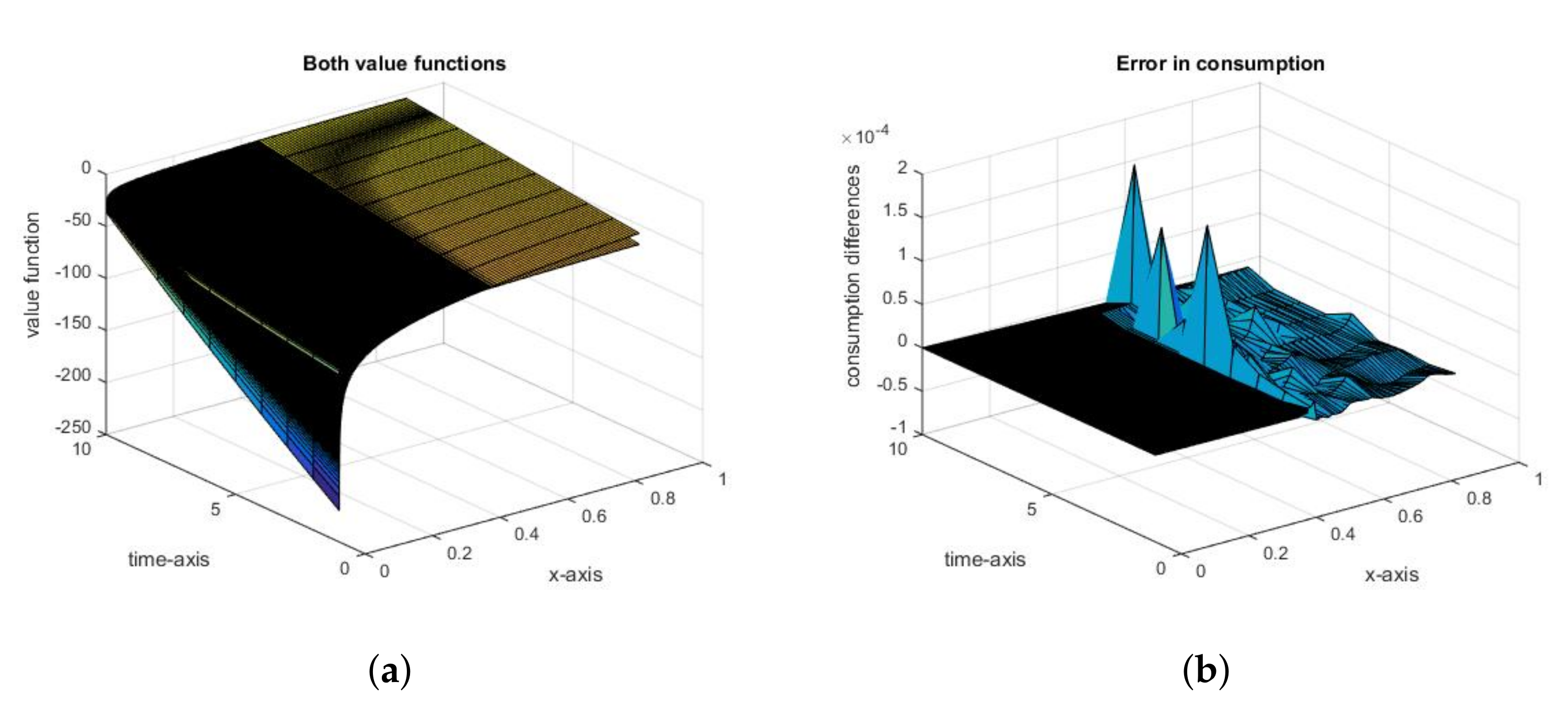
As we can see in Figure 1a, there is a substantial difference between the actual and numerical value functions for two regions of the set of states x: close to 0, the point of a singularity of the actual value function, where the approximate value function is substantially greater, and the interval $(\frac{1}{2},1],$ at which the grid is sparse and the approximate value function is substantially less. In fact, using numerical methods for problems with known points of singularities and not making the grid substantially finer as it converges to the singularity point of the calculated function means that we purposely leave the grid too sparse also for this region. Thus, our procedure means that we a priori allowed the value function to have errors substantially larger on some regions than inherent errors resulting from using numerical methods (if appropriate grids are used).

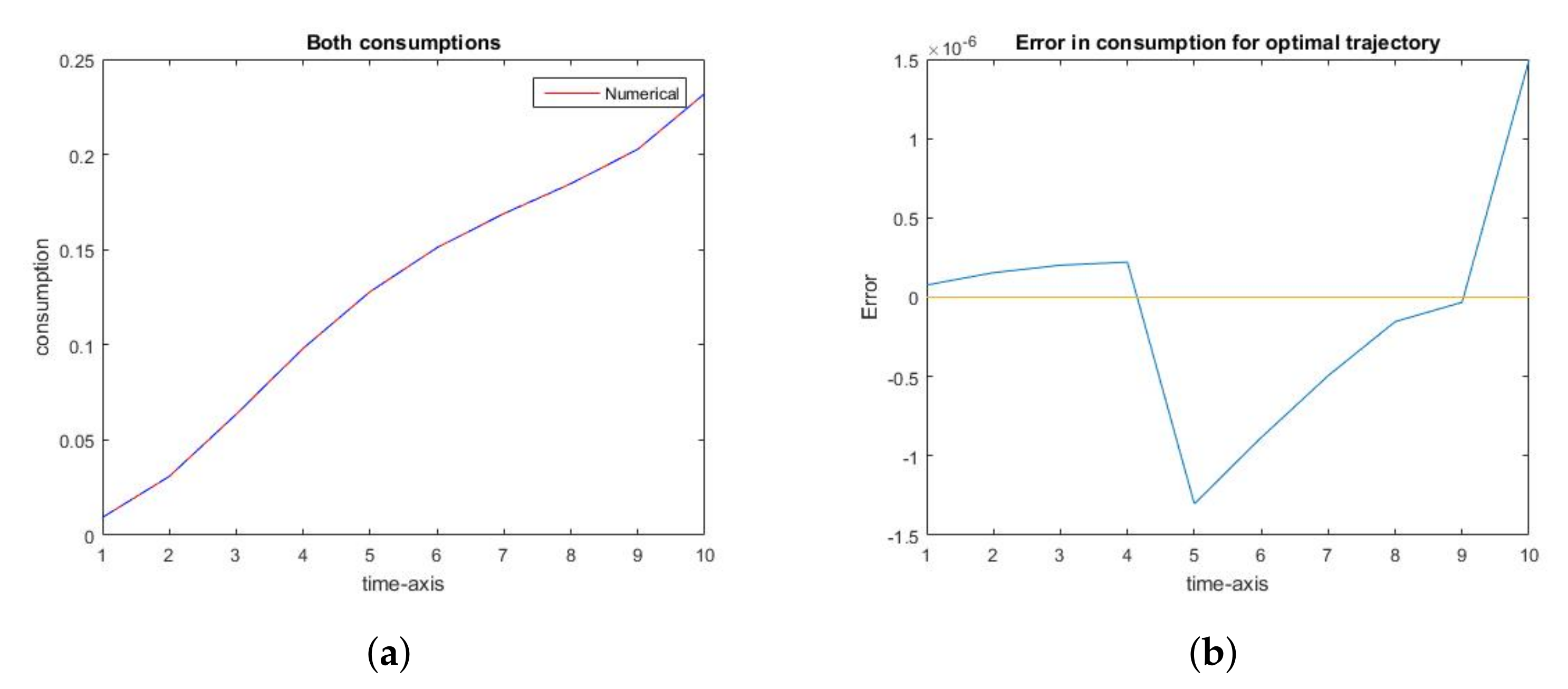
Despite those differences, both numerical and actual consumptions are apparently identical with errors of rank ${10}^{-4}$ (see Figure 1b, mainly at the region with the sparse grid).

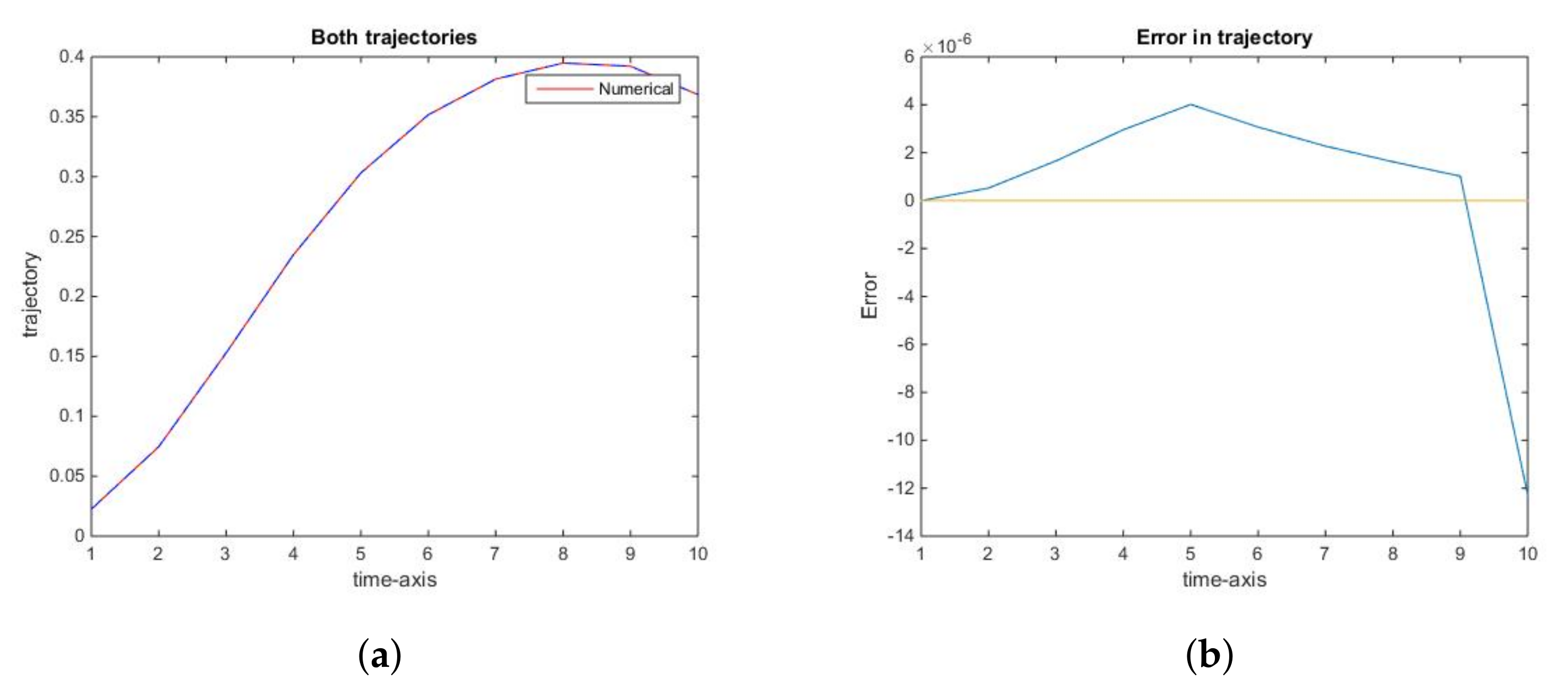
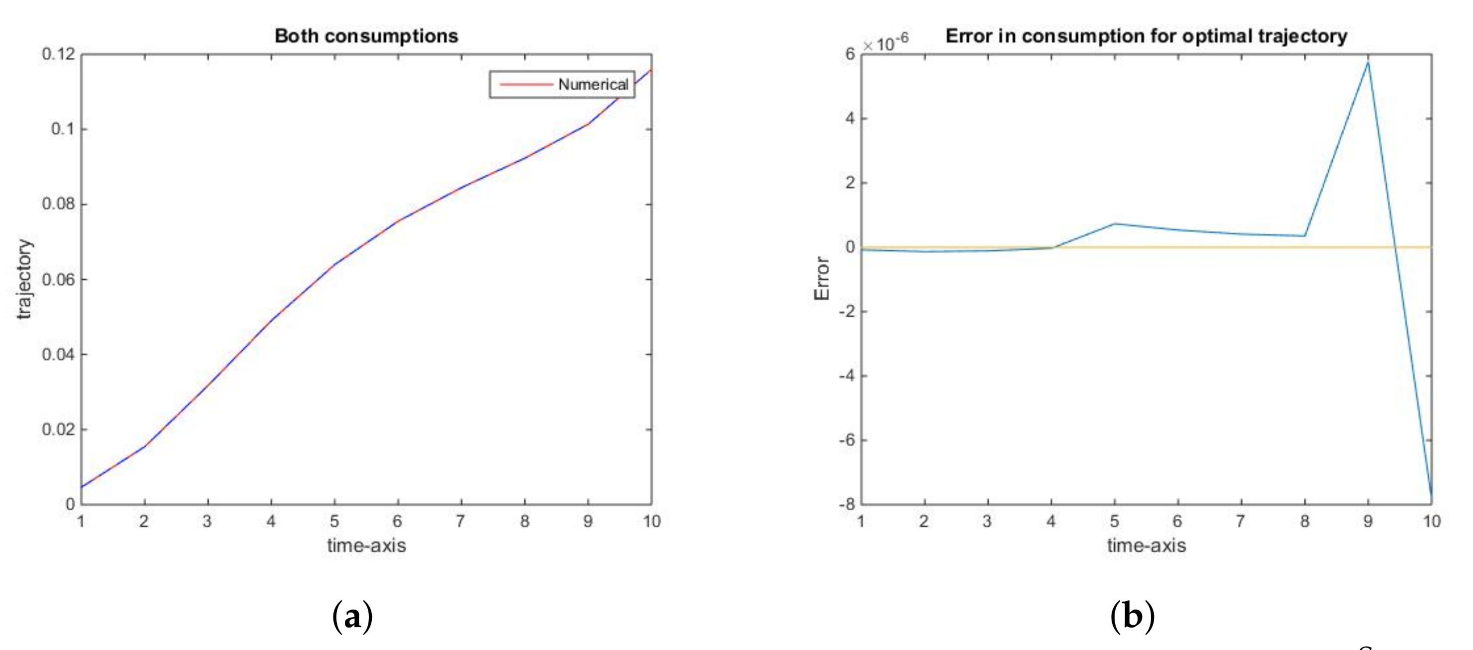
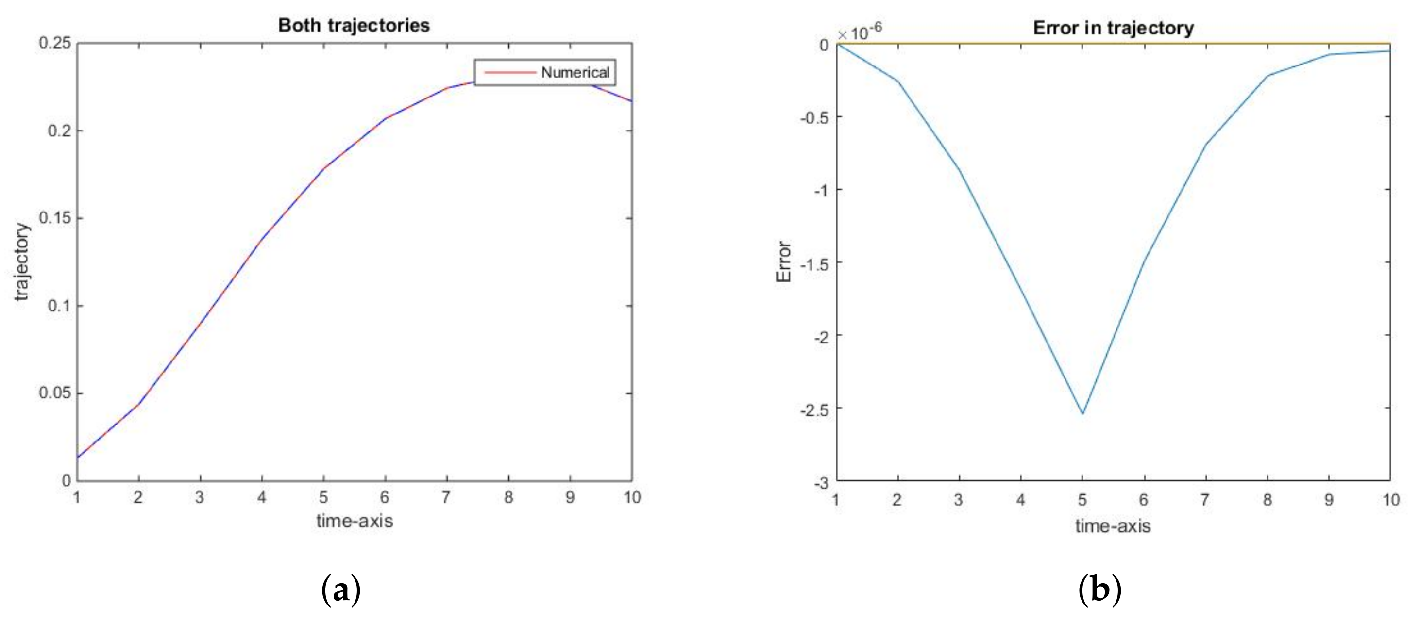
Similarly, the optimal trajectory, as well as the optimal consumption along it, are apparently identical to their numerically computed counterparts (Figure 2a and Figure 3a). In this case, the rank of error decreases to ${10}^{-6}$ (Figure 2b and Figure 3b). This fact is explained by Theorem 1, especially 1c). Thus, there is no need to refine the grid for x at the interval $(\frac{1}{2},1],$ at which it is sparse, as well as on the set of points close to the singularity at 0, since neither numerical nor analytic optimal trajectory has a non-empty intersection with those sets.

2.2.2. Nash Equilibrium

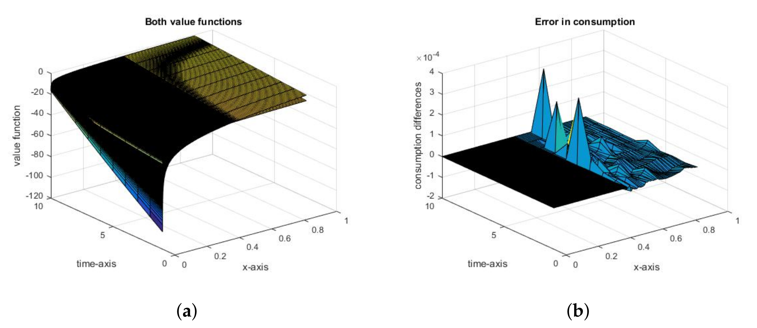
Analogously, for the Nash equilibrium, when we compare the actual results with the results of the numerical analysis, we have the same observations: the difference between the value functions (Figure 4a) is large on the same regions as for the social optimum, with apparently equal consumptions, $c^N(x,t)$ of error of rank ${10}^{-4}$ (Figure 4b), with two ranks having better accuracy of the Nash equilibrium consumption and state trajectories (Figure 5a and Figure 6a) with errors of rank ${10}^{-6}$ (Figure 5b and Figure 6b).

Note that the rank of accuracy for computing equilibria is the same as for the less complex problem of computing social optima. It means that the accuracy of finding the fixed point was very high. Thanks to the iterative procedure of refining the grid on small intervals (see Algorithm A2 described in the Appendix A), it was at a reasonable time cost.

2.3. General Conclusions from the Analysis of the Fish Wars Example

In both cases: the social optimum and the Nash equilibrium, we obtained a substantial error in the value functions on some intervals and high accuracy of the optimum/equilibrium trajectory and consumption path. This situation is rather unusual.

It is worth emphasizing that this holds not only for specific parameters and grids which we present graphically in this paper, but it is a more general rule. Even the first results obtained for the procedure of finding social optima, with quite few points of the grid, assumed to be used to test the code, before refinement of the grid on certain subsets of the set of states was introduced, revealed the same apparent paradox. While there was a considerable error in the value function, especially at the initial time and the regions close to boundaries of the set of states, the social optimum consumption path $c^S(t,X(t))$ as well as $X(t)$ was computed with unexpected (for this inaccuracy of V) accuracy.

A similar paradox took place while computing the Nash equilibrium. In spite of inaccurate computation of the value function close to the boundaries, the accuracy of computing the equilibrium path is comparable to the distance between the grid points for the sum of decisions of the other players o—the maximal precision that can be expected.

This has been obtained although we haven’t used knowledge about the actual value function and optimal strategy/equilibrium specific to this model while preparing the code for the numerical part, in order to be able to assess the applicability of this approach to a wider class of problems with similar properties.

The only information that we have used is the fact that the value function is continuous, regular for $x>0$ and $V(t,0)=-\infty$, the optimal trajectory remains below a certain level, (here, we took $\frac{1}{2}$) whenever the initial condition $x_0$ is below this level and it is over some small $ϵ>0$ whenever $x_0$ is, while, in computation of equilibrium, we have also used the fact that the best response of a player is a decreasing function of joint consumption of the others and that the equilibrium exists.

3. When and What Kind of Inaccuracies in Computation or Calculation of the Value Function Do Not Propagate on the Optimal Path in Dynamic Optimization Problems

In this section, we return to the general theoretical motivation of this paper, which is the explanation when paradoxes similar to those obtained for the Motivating Example in Section 2.3: high accuracy of derived optimal state trajectory and consumption path despite the inaccuracy of the corresponding value function on some intervals.

We want to emphasize that a situation in which substantial inaccuracy in a calculation of the value function does not propagate on the optimum path is very unusual. There are examples of a sequence of, regarded as regular, linear quadratic optimization problems, in which an error in calculation of the value function and the resulting “candidate for the optimal control”, for which the Bellman sufficient condition is fulfilled besides an interval with a length converging to zero as some parameter converges to zero that result in false value function and false optimal control on a considerable part of the set of states (Singh and Wiszniewska-Matyszkiel [9]).

We can prove the following theorems, which allow, in a very general environment of dynamic optimization problems, to determine the type of errors in approximation of the value function—either resulting from using numerical computation with low accuracy on some sets, or from replacing the actual value function by some a priori estimation of it on some sets—which do not influence the accuracy of the optimal trajectory and the optimal control path, i.e., the trajectory of the optimal control along the corresponding trajectory.

We consider any discrete time dynamic optimization problem:

• with the time set $\{0,1,\dots \}$ or $\{0,1,\dots ,T\}$, denoted by $\mathbb{T}$; the finite or infinite horizon is denoted by T;
• with discount factor $\beta \in (0,1]$;
• the set of states $\mathbb{X}$;
• the set of control parameters $\mathbb{C}$;
• the current payoff function $P:\mathbb{T}\times \mathbb{X}\times \mathbb{C}\to \mathbb{R}\cup \{-\infty \}$;
• where we consider the feedback controls $c:\mathbb{T}\times \mathbb{X}\to \mathbb{C}$ (which, if independent of time, are denoted as $c:\mathbb{X}\to \mathbb{C}$)
• with admissibility constraint $c(t,x)\in C(t,x)$ for all $t,x$ and for $C:\mathbb{T}\times \mathbb{X}⊸\mathbb{C}$; the set of admissible controls is denoted by $\mathfrak{C}$, and
• the transformation of the state variable is given by a function $\varphi :\mathbb{T}\times \mathbb{X}\times \mathbb{C}\to \mathbb{X}$ or, more generally
  $\varphi :\mathbb{T}\times \mathbb{X}\times \mathbb{C}\to \tilde{\mathbb{X}}\supseteq \mathbb{X}$ with $\varphi (t,x,c)\in \mathbb{X}$ for all $(t,x,c)\in \mathbb{T}\times \mathbb{X}\times \mathbb{C}$ with $c\in C(t,x)$. In the latter case, there is no need to specify $\tilde{X}$, as it does not influence the results.
• In the case when the time horizon is finite, we also consider a terminal payoff given by a function $G:\mathbb{X}\to \mathbb{R}\cup \{-\infty \}$, paid after the termination of the game.

The aim is to maximize, given $t_0\in \mathbb{T}$ and $x_0\in \mathbb{X}$, the objective functional $J(t_0,x_0,c)$ over the set of admissible controls $\mathfrak{C}$, where $J:\mathbb{T}\times \mathbb{X}\times \mathfrak{C}\to \mathbb{R}\cup \{-\infty \}$ is defined by

• $J(t_0,x_0,c)={\displaystyle \sum _{t=t_0}^{\infty }}P(t,X(t),c(t,X(t))){\beta }^{t-t_0}$ for the infinite time horizon, while
• $J(t_0,x_0,c)={\displaystyle \sum _{t=t_0}^T}P(t,X(t),c(t,X(t))){\beta }^{t-t_0}+G(X(T+1)){\beta }^{T+1-t_0}$ for a finite time horizon T,
• where the trajectory X corresponding to c is given by $X(t+1)=\varphi (t,X(t),c(t,X(t)))$
  with the initial condition $X(t_0)=x_0$.
• Whenever we want to emphasize the dependence of X on a control c, we write $X^c$, if we want to emphasize the dependence of X on the initial condition, we write $X_{t_0,x_0}$, while $X_{t_0,x_0}^c$ if we want to emphasize both.
• We assume that the problem is such that J is always well defined although it may be $\pm \infty$.
• We restrict the set of initial conditions to $x_0\in {\mathbb{X}}_0\subset \mathbb{X}$.

In the finite time horizon case, the necessary and sufficient condition for a function $V:(\mathbb{T}\cup \{T+1\})\times \mathbb{X}\to \mathbb{R}\cup \{-\infty \}$ to be the value function, i.e., to fulfill for every $(t,x)$, $V(t,x)=\underset{c\in \mathfrak{C}}{sup}J(t,x,c)$ and an admissible control $\overline{c}$ to be the optimal control, is the Bellman equation (see, e.g., Bellman [42], Blackwell [43], Stokey and Lucas [1] Başar and Olsder [44] or Haurie, Krawczyk and Zaccour [40] for various versions)

$$V(t,x)=\underset{c\in C(t,x)}{max}P(t,x,c)+\beta V(t+1,\varphi (t,x,c))\mathrm{for}\mathrm{all}t\in \mathbb{T},x\in \mathbb{X};$$

(3)

with the terminal condition

$$V(T+1,x)=G(x)\mathrm{for}\mathrm{all}x\in \mathbb{X}$$

(4)

and the inclusion

$$\overline{c}(t,x)\in \underset{c\in C(t,x)}{Argmax}P(t,x,c)+\beta V(t+1,\varphi (t,x,c))\mathrm{for}\mathrm{all}t\in \mathbb{T},x\in \mathbb{X}.$$

(5)

For the infinite time horizon optimization, the Bellman Equation (3) and the inclusion (5) remain the necessary condition, they also consitute a sufficient condition with certain terminal condition: usually, the standard terminal condition (see, e.g., Stokey, Lucas and Prescott [1], Theorems 4.2–4.4)

$$\underset{t\to \infty }{lim\; sup}{\beta }^{t}V(t,X(t))=0\mathrm{for}\mathrm{every}\mathrm{admissible}\mathrm{trajectory}\mathrm{X}.$$

(6)

Obviously, in the infinite time horizon version of our motivating example, the standard terminal condition (6) does not hold, so it has to be replaced by a weaker one, which, together with the Bellman Equation (3) and the inclusion (5), forms a sufficient condition (Wiszniewska-Matyszkiel [45], Theorem 1):

$$\begin{array}{c}\hfill \underset{t\to \infty }{lim\; sup}V(t,X(t)){\beta }^t\le 0\mathrm{for}\mathrm{every}\mathrm{admissible}\mathrm{trajectory}\mathrm{X}\mathrm{and}\end{array}$$

(7)

$$\begin{array}{c}\hfill \underset{t\to \infty }{lim\; sup}V(t,X(t)){\beta }^t<0\Rightarrow J(\overline{t},\overline{x},c)=-\infty \\ \hfill \mathrm{for}\mathrm{every}(\overline{t},\overline{x})\in \mathbb{T}\times \mathbb{X}\mathrm{and}\mathrm{every}\mathrm{control}c\mathrm{such}\mathrm{that}X=X_{\overline{t},\overline{x}}^c.\end{array}$$

(8)

Terminal conditions (7) and (8) have been proven to be necessary in a large class of optimal control problems including Fish Wars in Wiszniewska-Matyszkiel and Singh [3].

We introduce the following notation:

• V—the actual value function of the dynamic optimization problem;
• $V^{\mathrm{approx}}$—another function regarded as an approximation of V; it may be either a solution of a numerical procedure or the actual V with values on certain subsets replaced by another value, e.g., some constraint known a priori.
• ${\mathrm{RHS}}_{t,x}(c)=P(t,x,c)+\beta V(t+1,\varphi (t,x,c))$—the maximized function on the right-hand side of the Bellman Equation bellman-general (as a function of c).
• ${\mathrm{RHS}}_{t,x}^{\mathrm{approx}}(c)=P(t,x,c)+\beta V^{\mathrm{approx}}(t+1,\varphi (t,x,c))$—the maximized function on the right-hand side of the Bellman Equation (3) with V replaced by $V^{\mathrm{approx}}$ (as a function of c).
• $\mathrm{OPT}$—the set of optimal controls; we assume that it is non-empty.
• ${\mathrm{OPT}}^{\mathrm{approx}}$—the set of controls $\tilde{c}\in \mathfrak{C}$ such that $\tilde{c}(t,x)\in \underset{c\in \mathbb{C}}{Argmax}{\mathrm{RHS}}_{t,x}^{\mathrm{approx}}(c)$; we assume that it is non-empty.
• $\mathsf{\Omega }=\{(t,x):X_{t_0,x_0}^{\overline{c}}(t)=x\mathrm{for}\mathrm{some}\overline{c}\in \mathrm{OPT}\mathrm{and}{x}_0\in {\mathbb{X}}_0\}$.
• For $\overline{c}\in \mathfrak{C}$, ${\mathsf{\Omega }}^{\overline{c}}=\{(t,x):X_{t_0,x_0}^{\overline{c}}(t)=x\mathrm{for}\mathrm{some}{x}_0\in {\mathbb{X}}_0$}.
• ${\mathsf{\Omega }}^{\mathrm{approx}}=\{(t,x):X_{t_0,x_0}^{\tilde{c}}(t)=x\mathrm{for}\mathrm{some}\tilde{c}\in {\mathrm{OPT}}^{\mathrm{approx}}\mathrm{and}{x}_0\in {\mathbb{X}}_0\}$.

We can state the following theorem, explaining the apparent paradox of low errors in the computation of the optimal control path despite substantial errors in the computation of the value function in our Motivating Example.

Theorem 1.

Assume that either the horizon is finite or the terminal condition (7) and (8) hold for V.

Assume also that one of the following holds:

a) $V(t,x)=V^{\mathrm{approx}}(t,x)$ for all $(t,x)\in {\mathsf{\Omega }}^{\mathrm{approx}}$, and $V(t,x)\le V^{\mathrm{approx}}(t,x)$ for all $(t,x)\in \mathbb{T}\times \mathbb{X}$;

b) $V(t,x)=V^{\mathrm{approx}}(t,x)$ for all $(t,x)\in \mathsf{\Omega }$, and $V(t,x)\ge V^{\mathrm{approx}}(t,x)$ for all $(t,x)\in \mathbb{T}\times \mathbb{X}$;

c) $V(t,x)=V^{\mathrm{approx}}(t,x)$ for all $(t,x)\in \mathsf{\Omega }\cup {\mathsf{\Omega }}^{\mathrm{approx}}$.

Then, $\mathsf{\Omega }={\mathsf{\Omega }}^{\mathrm{approx}}$, for every $\overline{c}\in \mathrm{OPT}$ there exist $\tilde{c}\in {\mathrm{OPT}}^{\mathrm{approx}}$ such that $\tilde{c}{{|}_{\mathsf{\Omega }}=\overline{c}|}_{\mathsf{\Omega }}$ and for every $\tilde{c}\in {\mathrm{OPT}}^{\mathrm{approx}}$ there exist $\overline{c}\in \mathrm{OPT}$ such that $\tilde{c}{{|}_{\mathsf{\Omega }}=\overline{c}|}_{\mathsf{\Omega }}$.

To prove Theorem 1, we formulate the following lemmata.

Lemma 1.

Consider an arbitrary set $\mathbb{C}$ and two functions $f,g:\mathbb{C}\to \overline{\mathbb{R}}$ with $f(c)=g(c)$ for all $c\in Argmaxf\ne Ø$ and $f(c)\ge g(c)$ otherwise.

Then, $Argmaxf=Argmaxg$.

Proof. 

Take $\overline{c}\in Argmaxf$ and any other c.

By the assumptions, $g(c)\le f(c)\le f(\overline{c})=g(\overline{c})$. Thus, $\overline{c}\in Argmaxg$.

Next, take $\tilde{c}\in Argmaxg$ and assume that $\tilde{c}\notin Argmaxf$. Take $\overline{c}\in Argmaxf$.

By the assumptions, $g(\overline{c})\le g(\tilde{c})\le f(\tilde{c})<f(\overline{c})=g(\overline{c})$, which is a contradiction. □

Lemma 2.

Consider an arbitrary set $\mathbb{C}$ and two functions $f,g:\mathbb{C}\to \overline{\mathbb{R}}$ with $f(c)=g(c)$ for all $c\in Argmaxf\cup Argmaxg$ with both $Argmaxf,Argmaxg\ne Ø$.

Then, $Argmaxf=Argmaxg$.

Proof. 

Take $\tilde{c}\in Argmaxg$ and $\overline{c}\in Argmaxf$.

By the assumptions, $f(\tilde{c})\le f(\overline{c})=g(\overline{c})\le g(\tilde{c})=f(\tilde{c})$, which implies that $f(\tilde{c})=f(\overline{c})$ and $g(\overline{c})=g(\tilde{c})$. Thus, $\tilde{c}\in Argmaxf$ and $\overline{c}\in Argmaxg$. □

Proof of Theorem 1.

We start by noting that if $(t,x)\in \mathsf{\Omega }$, then

$$\mathrm{for}\mathrm{all}\overline{c}\in \underset{c\in C(t,x)}{Argmax}{\mathrm{RHS}}_{t,x}(c),(t+1,\varphi (t,x,\overline{c}))\in \mathsf{\Omega },$$

(9)

and if $(t,x)\in {\mathsf{\Omega }}^{\mathrm{approx}}$, then

$$\mathrm{for}\mathrm{all}\tilde{c}\in \underset{c\in C(t,x)}{Argmax}{\mathrm{RHS}}_{t,x}^{\mathrm{approx}}(c),(t+1,\varphi (t,x,\tilde{c}))\in {\mathsf{\Omega }}^{\mathrm{approx}}.$$

(10)

The proof will be by induction over t.

Together with $\mathsf{\Omega }={\mathsf{\Omega }}^{\mathrm{approx}}$, we prove that $\underset{c\in C(t,x)}{Argmax}{\mathrm{RHS}}_{t,x}(c)=\underset{c\in C(t,x)}{Argmax}{\mathrm{RHS}}_{t,x}^{\mathrm{approx}}(c)$ for all $(t,x)\in \mathsf{\Omega }$ (and, consequently, for all $(t,x)\in {\mathsf{\Omega }}^{\mathrm{approx}}$).

First, consider $t=t_0$ and arbitrary $x\in {\mathbb{X}}_0$.

In this case, $\mathsf{\Omega }\cap \{(t,y)\in \mathbb{T}\times \mathbb{X}:t\le t_0\}=\{t_0\}\times {\mathbb{X}}_0={\mathsf{\Omega }}^{\mathrm{approx}}\cap \{(t,x)\in \mathbb{T}\times \mathbb{X}:t\le t_0\}$ in all the cases a)–c).

Next, consider any $t\ge t_0$ and any x such that $(t,x)\in \mathsf{\Omega }$.

Assume that $\mathsf{\Omega }\cap \{(k,y)\in \mathbb{T}\times \mathbb{X}:k\le t\}={\mathsf{\Omega }}^{\mathrm{approx}}\cap \{(k,y)\in \mathbb{T}\times \mathbb{X}:k\le t\}$.

By Lemma 1 applied to the functions ${\mathrm{RHS}}_{t,x}^{\mathrm{approx}}$ and ${\mathrm{RHS}}_{t,x}$, and Equations (10) and (9), respectively, we obtain $\underset{c\in C(t,x)}{Argmax}{\mathrm{RHS}}_{t,x}(c)=\underset{c\in C(t,x)}{Argmax}{\mathrm{RHS}}_{t,x}^{\mathrm{approx}}(c)$ in cases a) and b).

By Lemma 2 applied to the functions ${\mathrm{RHS}}_{t,x}^{\mathrm{approx}}$ and ${\mathrm{RHS}}_{t,x}$, and any of Equation (10) or (9), we obtain that $\underset{c\in C(t,x)}{Argmax}{\mathrm{RHS}}_{t,x}(c)=\underset{c\in C(t,x)}{Argmax}{\mathrm{RHS}}_{t,x}^{\mathrm{approx}}(c)$ in case c).

Consequently, in all cases a)–c), $\mathsf{\Omega }\cap \{(k,y)\in \mathbb{T}\times \mathbb{X}:k\le t+1\}={\mathsf{\Omega }}^{\mathrm{approx}}\cap \{(k,y)\in \mathbb{T}\times \mathbb{X}:k\le t+1\}$.

This ends the proof that $\mathsf{\Omega }={\mathsf{\Omega }}^{\mathrm{approx}}$ and that $\underset{c\in C(t,x)}{Argmax}{\mathrm{RHS}}_{t,x}(c)=\underset{c\in C(t,x)}{Argmax}{\mathrm{RHS}}_{t,x}^{\mathrm{approx}}(c)$ for all $(t,x)\in \mathsf{\Omega }$.

Take any $\tilde{c}\in {\mathrm{OPT}}^{\mathrm{approx}}$. Define $\overline{c}\in \mathfrak{C}$ such that $\overline{c}(t,x)=\tilde{c}(t,x)$ for all $(t,x)\in \mathsf{\Omega }$ and $\overline{c}(t,x)$ being any selection from $\underset{c\in C(t,x)}{Argmax}{\mathrm{RHS}}_{t,x}(c)$, otherwise.

The terminal condition either (4) or (7) and (8) is fulfilled.

By the fact that $\underset{c\in C(t,x)}{Argmax}{\mathrm{RHS}}_{t,x}(c)=\underset{c\in C(t,x)}{Argmax}{\mathrm{RHS}}_{t,x}^{\mathrm{approx}}(c)$ also the Bellman equation is fulfilled, so $\overline{c}\in \mathrm{OPT}$.

Next, take any $\overline{c}\in \mathrm{OPT}$. Define $\tilde{c}\in \mathfrak{C}$ such that $\tilde{c}(t,x)=\overline{c}(t,x)$ for all $(t,x)\in \mathsf{\Omega }$ and $\tilde{c}(t,x)$ being any selection from $\underset{c\in C(t,x)}{Argmax}{\mathrm{RHS}}_{t,x}^{\mathrm{approx}}(c)$, otherwise. Since $\underset{c\in C(t,x)}{Argmax}{\mathrm{RHS}}_{t,x}(c)=\underset{c\in C(t,x)}{Argmax}{\mathrm{RHS}}_{t,x}^{\mathrm{approx}}(c)$, by the definition, $\overline{c}\in {\mathrm{OPT}}^{\mathrm{approx}}$. □

Theorem 1 states that any error described by a), b), or c) does not influence the quality of computation or calculation of the optimal state trajectory of the state variable and the optimal control path, $c(t,X(t))$, i.e., the approximate X and $C(t,X(t))$ are the same as for an optimal control and every optimal control can be calculated using such an approximate value function and the result will be correct along the corresponding trajectory. Thus, overestimation of V on the set of points (i.e., states or time-state pairs) which never belong to the trajectory corresponding to the control defined by maximization of the Bellman equation with the approximate value function, as well as underestimation of the value function on the set of points which are suboptimal along the optimal trajectory, does not lead to any errors in calculation of the optimal consumption path and the optimal trajectory of the state variable. Similarly, this holds for any errors at points which are neither at the optimal trajectory nor the trajectory corresponding to the control defined by maximization of the Bellman equation with the approximate value function.

This is why we have purposely decreased the number of grid points in computation of the solutions in the Fish Wars example for $x>\frac{1}{2}$, although on this set there is a very visible difference between the actual and approximate value functions, in addition to us not caring about large, opposite in sign, differences between the value functions for x very close to 0.

Theorem 2.

Assume that either the horizon is finite or the terminal conditions (7) and (8) hold for V.

Consider a control $c\in \mathfrak{C}$.

Assume also that one of the following holds:

a) If $c\in {\mathrm{OPT}}^{\mathrm{approx}}$ and $V(t,x)=V^{\mathrm{approx}}(t,x)$ for all $(t,x)\in {\mathsf{\Omega }}^c$, and $V(t,x)\le V^{\mathrm{approx}}(t,x)$ for all $(t,x)\in \mathbb{T}\times \mathbb{X}$, then there exist $\overline{c}\in \mathrm{OPT}$ such that ${\mathsf{\Omega }}^{\overline{c}}={\mathsf{\Omega }}^c$ and ${c|}_{{\mathsf{\Omega }}^c}=\overline{c}{|}_{{\mathsf{\Omega }}^c}$.

b) If $c\in \mathrm{OPT}$ and $V(t,x)=V^{\mathrm{approx}}(t,x)$ for all $((t,x))\in {\mathsf{\Omega }}^c$, and $V(t,x)\ge V^{\mathrm{approx}}(t,x)$ all $(t,x)\in \mathbb{T}\times \mathbb{X}$, then there exist $\tilde{c}\in {\mathrm{OPT}}^{\mathrm{approx}}$ such that ${\mathsf{\Omega }}^{\tilde{c}}={\mathsf{\Omega }}^c$$\tilde{c}{{|}_{\mathsf{\Omega }}=c|}_{\mathsf{\Omega }}$.

Proof. 

Following almost the same lines as proof of Theorem 1, we only concentrate on a single control from $\mathrm{OPT}$ or ${\mathrm{OPT}}^{\mathrm{approx}}$. □

Illustration of Usefulness of Theorems 1 and 2 by Examples

For simplicity, we consider the social optimum problem and we show how Theorem 1 can be applied in order to simplify the computation of the social optimum.

We consider the social optimum in the Levhari and Mirman model, either with a finite horizon, like those analyzed in Section 2, or its infinite horizon version. In the analysis of the infinite horizon problem, we consider the value function and controls dependent on the state variable only, while in the finite horizon, they are dependent also on time.

To show that the method is general and it can be applied for the infinite time horizon, we introduce the limit game of our Motivating Example with the infinite time horizon.

Proposition 3.

Consider the game from Section 2 but with $T=+\infty$. The social optimum for the infinite horizon problem is $c_i^S(x)=\frac{x(1-\alpha \beta )}{n}$ with the value function $V_i^S(x)=n(A^S+B^{S}ln(x))$, for $A^S=\frac{1}{1-\beta }\left(\frac{\alpha \beta }{1-\alpha \beta }ln(\alpha \beta )+ln(1-\alpha \beta )-ln(n)\right)$ and $B^S=\frac{1}{1-\alpha \beta }$, while the Nash equilibrium is $c_i^N(x)=\left(\frac{1-\alpha \beta }{n(1-\alpha \beta )+\alpha \beta }\right)$, with the value function $V_i^N(x)=A^N+B^{N}ln(x)$ for $A^N=\frac{1}{1-\beta }\left(\frac{\alpha \beta }{1-\alpha \beta }ln\left(\frac{\alpha \beta }{n(1-\alpha \beta )+\alpha \beta }\right)+ln\left(\frac{1-\alpha \beta }{n(1-\alpha \beta )+\alpha \beta }\right)\right)$ and $B^N=\frac{1}{1-\alpha \beta }$.

Proof. 

The formulae have been proposed by Levhari, Mirman [15], and Okuguchi [16]. Checking that the Bellman Equations (3) and (5) hold is just a substitution. Nevertheless, the proofs of [15,16] lack checking the necessary terminal conditions (7) and (8), while the standard sufficient terminal condition (6) does not hold.

Thus, to complete the proof, we check the terminal conditions (7) and (8). Equation (7) is immediate by the fact that $ln(c_i)\le 0$ for all admissible $c_i$.

To prove Equation (8) for the social optimum, we consider a strategy c for which $\underset{t\to \infty }{lim\; sup}{\beta }^t·V^S(X^c(t))<0$. Thus, there exists a subsequence $t_k$ such that $\underset{k\to \infty }{lim}{\beta }^{t_k}{V}^S(X^c(t_k))<0$. Thus, $\underset{k\to \infty }{lim}{\beta }^{t_k}ln(X^c(t_k))<0$.

${\displaystyle \sum _{i=1}^n}{J}_i\left(t_0,x_0,c_i,c_{\sim i}\right)={\displaystyle \sum _{i=1}^n}{\displaystyle \sum _{t=t_0}^{\infty }}{\beta }^{t-t_0}ln(c_i(X^c(t)))\le {\displaystyle \sum _{i=1}^n}{\displaystyle \sum _{k=0}^{\infty }}{\beta }^{t_k-t_0}ln(c_i(X^c(t_k)))$

$\le {\displaystyle \sum _{i=1}^n}{\displaystyle \sum _{k=0}^{\infty }}{\beta }^{t_k-t_0}ln(\frac{X^c(t_k))}{n}\to -\infty$.

The proof for the Nash equilibrium is analogous. □

Example 1.

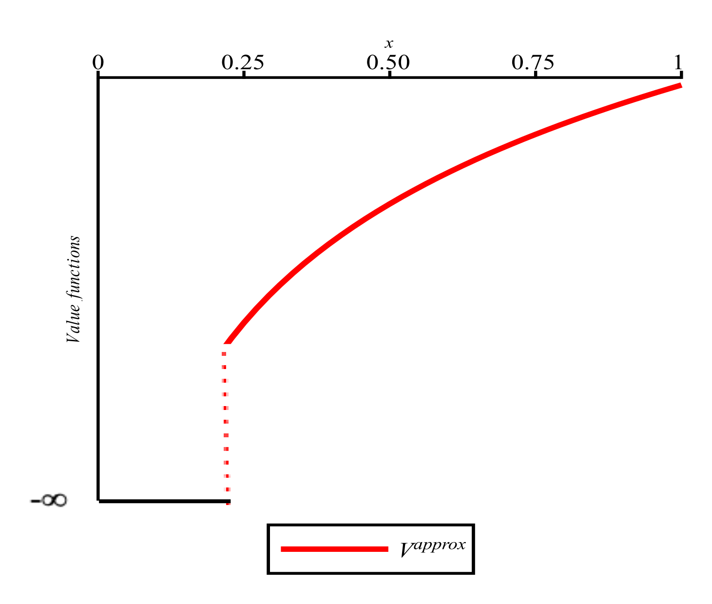
Assume that some preliminary analysis has been done for the problem resulted in finding an $ϵ<x_0$ for which it has been proven that the optimal trajectory $X(t)>ϵ$ for all t. Such an ϵ obviously exists.

Changing V by assigning $V^{\mathrm{approx}}=-\infty$ for all $x<\frac{ϵ}{2}$ (see Figure 7) changes neither the optimal trajectory nor the optimal control path.

Thus, if we want to compute the optimal control, this substitution allows us to look for the social optimum and the value function for $x\ge \frac{ϵ}{2}$ only and to avoid problems resulting from inaccuracies resulting from closeness to the actual singularity.

Example 2. 

Assume again that some preliminary analysis done for the problem has resulted in finding an $ϵ<x_0$ for which we know that the optimal trajectory $X(t)>ϵ$ for all t.

Since $V(x)\ge J(t_0,x,c)$ for every control c, changing V by assigning $V^{\mathrm{approx}}(x)=J(t_0,x,\overline{c})$ for all $x<\frac{ϵ}{2}$, for any control $\overline{c}$ changes neither the optimal trajectory nor the optimal control path.

Thus, if we want to compute the optimal control, this substitution allows us to look for the value function for $x\ge \frac{ϵ}{2}$ only (and the resulting optimal control).

Example 3.

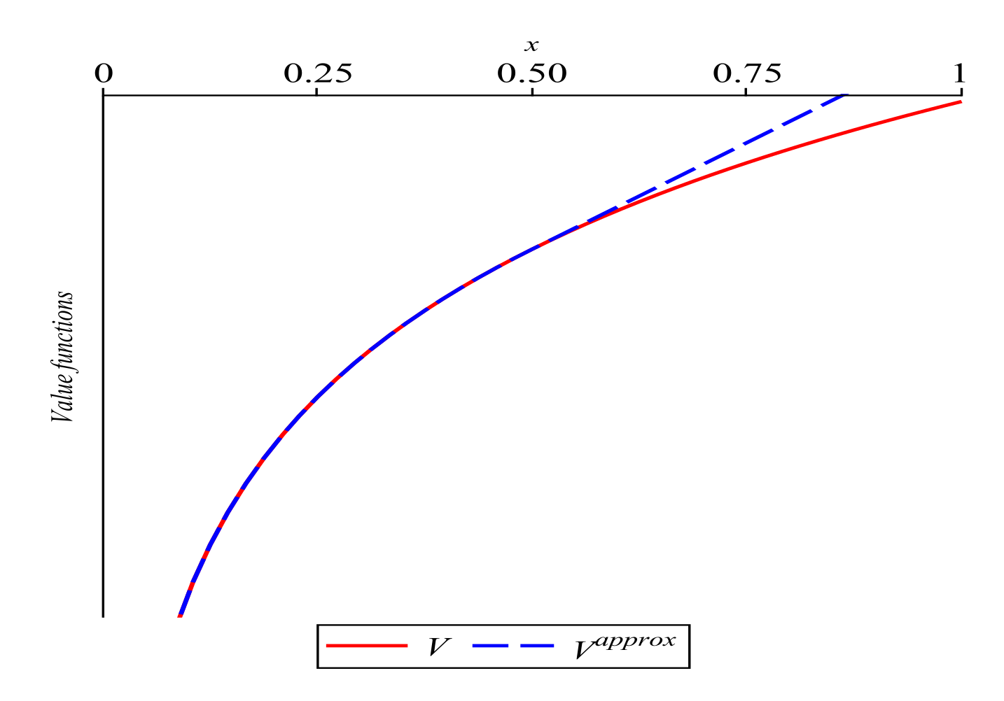
Assume that preliminary analysis done for the problem resulted in finding constants a and b for which we know that $ax+b$ is an upper bound for the value function for $x>\frac{1}{2}$ (see Figure 8) and in discovering the fact that if $x_0\le \frac{1}{2}-ϵ$, then, for all t, the optimal trajectory $X_{t_0,x_0}^{\overline{c}}(t)\le \frac{1}{2}-ϵ$.

If we change V by assigning $V^{\mathrm{approx}}(x)=ax+b$ for all $x>\frac{1}{2}$, and calculate the maximand $\tilde{c}$ of the right-hand side of the Bellman equation with $V^{\mathrm{approx}}$, then, if the trajectory $X_{t_0,x_0}^{\tilde{c}}(t)<\frac{1}{2}-ϵ$ for all t, then $\tilde{c}(t,X_{t_0,x_0}^{\tilde{c}}(t))$ is the accurate solution path.

Thus, if we want to compute the optimal control, this substitution allows us to restrict the computation of the value function for $x<\frac{1}{2}-ϵ$ with one restriction: it is proven that our result is really the optimal control only when for all $x_0<\frac{1}{2}-ϵ$, the computed $\tilde{c}$ is such that $X_{t_0,x_0}^{\tilde{c}}(t)<\frac{1}{2}-ϵ$ for all t.

Example 4.

To define our next $V^{\mathrm{approx}}$, we consider two small numbers $1>>{ϵ}_1>ϵ>0$ (${ϵ}_1$ is fixed, while ϵ will be adjusted) and some obvious overestimation $V^{+}\ge V$, e.g., $V^{+}(x)=lnx$. Next, we define $V^{ϵ}:[ϵ,1]\to \mathbb{R}$ as the solution the Bellman equation with one change—$V({(x-\sum c_i)}^{\alpha })$ in its rhs is replaced by $V^{+}({(x-\sum c_i)}^{\alpha })$ whenever ${(x-\sum c_i)}^{\alpha }<ϵ$—that fulfills the terminal conditions (7) and (8). Note that such a solution obviously exists and it is unique and it coincides with the actual value function of the problem with an additional constraint on controls ${(x-\sum c_i)}^{\alpha }\ge ϵ$ besides a small neighbourhood of 0 if ϵ is small enough.

If ϵ is such that the solution $V^{{ϵ}_2}$ is invariant with respect to ${ϵ}_2$ for $0<{ϵ}_2<ϵ$ on the interval $[{ϵ}_1,1]$, then we can consider

$$V^{\mathrm{approx}}(x)=\left\{\begin{array}{cc}{V}^{+}(x)\hfill & \mathrm{if}x<ϵ,\hfill \\ V^{ϵ}(x)\hfill & otherwise.\hfill \end{array}\right.$$

This assumption is easy to check—it is enough to find ϵ for which the maximum in the rhs of the Bellman equation with the corresponding $V^{\mathrm{approx}}$ is attained only for c for which ${(x-\sum c_i)}^{\alpha }\ge {ϵ}_1$ whenever $x\ge {ϵ}_1$. For our example, it obviously holds, since $V^{+}(x)\to -\infty$ as $x\to 0$.

Then, every control $\tilde{c}$ maximizing ${\mathrm{RHS}}_{t,x}^{\mathrm{approx}}$ coincides with the actual optimal control whenever $x_0\ge {ϵ}_1$.

Note that, in this case, the only knowledge that we used about the value function is its obvious overestimation $V^{+}$.

A theorem stating how to find over- and under-estimations of the actual value function by solving some inequalities analogous to the Bellman equation with the terminal conditions (7) and (8) are in, e.g., Kamihigashi [8].

Those two types of over- and under-estimations of the value functions in the infinite horizon may also appear as a result of approximating the infinite horizon value function by its finite horizon truncations—for nonnegative payoffs, they are underestimations while, for the nonpositive payoffs, they are overestimations—or a result of an iterative procedure. Such procedures of estimating the value function by value iterations is currently being extensively studied in the infinite horizon problems (for various versions, see, e.g., Martins-da-Rocha and Vailakis [4] and Le Van and Morhaim [5] for continuous problems and Kamihigashi [8] for discontinuous problems).

4. When and What Kind of Inaccuracies in Computation or Calculation of the Value Functions Do Not Propagate on the Nash Equilibrium Path in Dynamic Games

Here, we extend the results of Section 3 for Nash equilibria in dynamic games.

We consider a discrete time dynamic game:

• with n players;
• with finite or infinite horizon T;
• the time set $\{0,1,\dots \}$ or $\{0,1,\dots ,T\}$ is denoted by $\mathbb{T}$;
• with discount factor $\beta \in (0,1]$;
• the set of states $\mathbb{X}$;
• players’ sets of decisions ${\mathbb{C}}_i$
• with notation ${\mathbb{C}}_{\sim i}={\times }_{j\ne i}{\mathbb{C}}_j$ and $\mathbb{C}={\times }_{j=1,\dots ,n}{\mathbb{C}}_j$;
• players’ current payoff functions $P_i:\mathbb{T}\times \mathbb{X}\times {\mathbb{C}}_i\times {\mathbb{C}}_{\sim i}\to \mathbb{R}\cup \{-\infty \}$;
• where we consider feedback strategies $c_i:\mathbb{T}\times \mathbb{X}\to {\mathbb{C}}_i$ (if independent of time, they are written as $c_i:\mathbb{X}\to {\mathbb{C}}_i$)
• which fulfill the admissibility constraint $c_i(t,x)\in C_i(t,x)$ for all $t,x$ and for $C_i:\mathbb{T}\times \mathbb{X}⊸{\mathbb{C}}_i$.
• We denote the set of admissible strategies of player i by ${\mathfrak{C}}_i$, while the set of strategies of the remaining players by ${\mathfrak{C}}_{\sim i}$ and the set of strategy profiles by $\mathfrak{C}$;
• For simplicity, we introduce the symbol $[c_i,{\overline{c}}_{\sim i}]$ to denote the profile at which player i chooses $c_i$ while the remaining players choose their strategies ${\overline{c}}_{\sim i}$, which are their strategies resulting from $\overline{c}$;
• the transformation of the state variable is determined by $\varphi :\mathbb{T}\times \mathbb{X}\times \mathbb{C}\to \mathbb{X}$ or, more generally,
  $\varphi :\mathbb{T}\times \mathbb{X}\times \mathbb{C}\to \tilde{\mathbb{X}}\supseteq \mathbb{X}$ with $\varphi (t,x,c)\in \mathbb{X}$ for all $(t,x,c)\in \mathbb{T}\times \mathbb{X}\times \mathbb{C}$ with $c\in C(t,x)$. Specifying $\tilde{X}$ is unnecessary since it does not influence the results.
• In the case when the time horizon is finite, we also consider terminal payoffs given by functions $G_i:\mathbb{X}\to \mathbb{R}\cup \{-\infty \}$, paid after termination of the game.
• The payoff is $J_i\left(t_0,x_0,c_i,c_{\sim i}\right)={\displaystyle \sum _{t=t_0}^{\infty }}{\beta }^{t-t_0}{P}_i\left(t,X(t),c_i(t,X(t)),c_{\sim i}(t,X(t))\right)$ in the case of the infinite time horizon
• and $J_i\left(t_0,x_0,c_i,c_{\sim i}\right)={\displaystyle \sum _{t=t_0}^T}{\beta }^{t-t_0}{P}_i\left(t,X(t),c_i(t,X(t)),c_{\sim i}(t,X(t))\right)+{\beta }^{T+1-t_0}G(X(T+1))$ for finite time horizon T,
• where the trajectory X corresponding to a strategy profile c is given by
  $X(t+1)=\varphi (t,X(t),c(t,X(t)))$ with the initial condition $X(t_0)=x_0$.
• Whenever we want to emphasize the dependence of X on a strategy $c_i$ of player i, we write $X^{c_i}$, if we want to emphasize the dependence of X on the initial condition, we write $X_{t_0,x_0}$, while $X_{t_0,x_0}^{c_i}$ if we want to emphasize both. If we also want to emphasize the strategies of the remaining players, we write $X_{t_0,x_0}^{[c_i,c_{\sim i}]}$, or $X_{t_0,x_0}^c$ whenever c denotes the whole profile.
• We assume that the problem is such that $J_i$ is always well defined although it may be $\pm \infty$.
• We restrict the initial condition to $x_0\in {\mathbb{X}}_0\subset \mathbb{X}$.

At a feedback Nash equilibrium, given strategies of the other players $c_{\sim i}\in {\mathfrak{C}}_{\sim i}$, the aim of each player is to maximize, for each $t_0\in \mathbb{T}$ and $x_0\in \mathbb{X}$, the objective functional $J_i\left(t_0,x_0,c_i,c_{\sim i}\right)$ over the set of admissible controls ${\mathfrak{C}}_i$. Formally, it can be defined as

Definition 2.

A feedback Nash equilibrium is a profile of strategies $\overline{c}$ such that for every player i, for every strategy $c_i$ of player i, for every $t_0$ and $x_0$,

$$J_i\left(t_0,x_0,c_i,{\overline{c}}_{\sim i}\right)\le J_i\left(t_0,x_0,{\overline{c}}_i,{\overline{c}}_{\sim i}\right).$$

First, consider a profile of strategies $\overline{c}$ and we fix the strategies of the others ${\overline{c}}_{\sim i}\in {\mathfrak{C}}_{\sim i}$.

We introduce the following notations:

• $V_i(·,·,{\overline{c}}_{\sim i}):\overline{\mathbb{T}}\times \mathbb{X}\to \overline{\mathbb{R}}$—the actual value function of the dynamic optimization problem of player i given ${\overline{c}}_{\sim i}$, i.e., $V_i(t,x,{\overline{c}}_{\sim i})=\underset{c_i\in {\mathfrak{C}}_i}{sup}{J}_i(t,x,c_i,c_{\sim i})$.
• $V_i^{\mathrm{approx}}(·,·,{\overline{c}}_{\sim i}):\overline{\mathbb{T}}\times \mathbb{X}\to \overline{\mathbb{R}}$—another function regarded as approximation of $V_i(·,·,{\overline{c}}_{\sim i})$; it may be either a solution of a numerical procedure or the actual $V_i(·,·,{\overline{c}}_{\sim i})$ with values on certain subsets replaced by another values, e.g., some constraints; we assume a priori that, in the finite time horizon T, $V_i^{\mathrm{approx}}(T+1,x,{\overline{c}}_{\sim i})=G(x)$.
• ${\mathrm{RHS}}_{i,t,x,{\overline{c}}_{\sim i}}(c_i)=P_i(t,x,c_i,{\overline{c}}_{\sim i}(t,x))+\beta V_i(t+1,\varphi (t,x,[c_i,{\overline{c}}_{\sim i}]),{\overline{c}}_{\sim i})$—the maximized function on the right-hand side of the Bellman Equation (3) rewritten to maximization of player i given ${\overline{c}}_{\sim i}$;
• ${\mathrm{RHS}}_{i,t,x,{\overline{c}}_{\sim i}}^{\mathrm{approx}}(c_i)=P_i(t,x,c_i,{\overline{c}}_{\sim i}(t,x))+\beta V_i^{\mathrm{approx}}(t+1,\varphi (t,x,[c_i,{\overline{c}}_{\sim i}]),{\overline{c}}_{\sim i})$—the maximized function on the right-hand side of the Bellman Equation (3) rewritten to maximization of player i given ${\overline{c}}_{\sim i}$ with $V_i$ replaced by $V_i^{\mathrm{approx}}$.
• ${\mathrm{BEST}}_i({\overline{c}}_{\sim i})$—the set of strategies of player i which are best responses to ${\overline{c}}_{\sim i}$; we assume that it is non-empty;
• ${\mathrm{BEST}}_i^{\mathrm{approx}}({\overline{c}}_{\sim i})$—the set of strategies ${\tilde{c}}_i$ such that
  ${\tilde{c}}_i(t,x)\in \underset{c_i\in C_i(t,x)}{Argmax}{\mathrm{RHS}}_{i,t,x,{\overline{c}}_{\sim i}}^{\mathrm{approx}}(c_i)$; we assume that it is non-empty;
• For $c_i\in {\mathfrak{C}}_i$: ${\mathsf{\Omega }}_i^{c_i}({\overline{c}}_{\sim i})=\{(t,x):X_{t_0,x_0}^{[c_i,{\overline{c}}_{\sim i}]}(t)=x\mathrm{for}\mathrm{some}{x}_0\in {\mathbb{X}}_0\}$;
• For $c\in \mathfrak{C}$: ${\mathsf{\Omega }}^c=\{(t,x):X_{t_0,x_0}^c(t)=x\mathrm{for}\mathrm{some}{x}_0\in {\mathbb{X}}_0\}$;
• ${\mathsf{\Omega }}_i({\overline{c}}_{\sim i})=\{(t,x):X_{t_0,x_0}^{[c_i,{\overline{c}}_{\sim i}]}(t)=x\mathrm{for}\mathrm{some}{c}_i\in {\mathrm{BEST}}_i({\overline{c}}_{\sim i})\mathrm{and}{x}_0\in {\mathbb{X}}_0\}$;
• ${\mathsf{\Omega }}_i^{\mathrm{approx}}({\overline{c}}_{\sim i})=\{(t,x):X_{t_0,x_0}^{[c_i,{\overline{c}}_{\sim i}]}(t)=x\mathrm{for}\mathrm{some}c\in {\mathrm{BEST}}_i^{\mathrm{approx}}({\overline{c}}_{\sim i}),x_0\in {\mathbb{X}}_0\}$.

We can state the following theorem, being an immediate corollary of Theorem 1.

Theorem 3.

Consider a profile $\overline{c}$ and assume that all players besides i play ${\overline{c}}_j$ and in the case of the infinite time horizon $V_i(·,·,{\overline{c}}_{\sim i})$ fulfills the terminal conditions (7) and (8).

Assume also that one of the following holds:

a) $V_i(t,x,{\overline{c}}_{\sim i})=V_i^{\mathrm{approx}}(t,x,{\overline{c}}_{\sim i})$ for all $(t,x)\in {\mathsf{\Omega }}_i^{\mathrm{approx}}({\overline{c}}_{\sim i})$ and $V_i(t,x,{\overline{c}}_{\sim i})\le V_i^{\mathrm{approx}}(t,x,{\overline{c}}_{\sim i})$, otherwise;

b) $V_i(t,x,{\overline{c}}_{\sim i})=V_i^{\mathrm{approx}}(t,x,{\overline{c}}_{\sim i})$ for all $(t,x)\in {\mathsf{\Omega }}_i({\overline{c}}_{\sim i})$ and $V_i(t,x)\ge V_i^{\mathrm{approx}}(t,x,{\overline{c}}_{\sim i})$, otherwise;

c) $V_i(t,x,{\overline{c}}_{\sim i},)=V_i^{\mathrm{approx}}(t,x,{\overline{c}}_{\sim i})$ for all $(t,x)\in {\mathsf{\Omega }}_i({\overline{c}}_{\sim i})\cup {\mathsf{\Omega }}_i^{\mathrm{approx}}({\overline{c}}_{\sim i})$.

Then, ${\mathsf{\Omega }}_i^{\mathrm{approx}}({\overline{c}}_{\sim i})={\mathsf{\Omega }}_i({\overline{c}}_{\sim i})$, for every ${\overline{c}}_i\in {\mathrm{BEST}}_i({\overline{c}}_{\sim i})$ there exist ${\tilde{c}}_i\in {\mathrm{BEST}}_i^{\mathrm{approx}}({\overline{c}}_{\sim i})$ such that ${\tilde{c}}_i{{|}_{{\mathsf{\Omega }}_i({\overline{c}}_{\sim i})}=\overline{c}|}_{{\mathsf{\Omega }}_i({\overline{c}}_{\sim i})}$ and for every ${\tilde{c}}_i\in {\mathrm{BEST}}_i^{\mathrm{approx}}({\overline{c}}_{\sim i})$ there exist ${\overline{c}}_i\in {\mathrm{BEST}}_i({\overline{c}}_{\sim i})$ such that ${\tilde{c}}_i{{|}_{{\mathsf{\Omega }}_i({\overline{c}}_{\sim i})}={\overline{c}}_i|}_{{\mathsf{\Omega }}_i({\overline{c}}_{\sim i})}$.

Proof. 

Immediately, by Theorem 1 applied to the optimization of player i given the strategies of the others ${\overline{c}}_{\sim i}$. □

Theorem 3 for $\overline{c}$ being the Nash equilibrium profile states that, given the initial state $x_0\in {\mathbb{X}}_0$ and correct expectation of the other players’ strategies ${\overline{c}}_{\sim i}$, overestimation of $V_i(t,x,{\overline{c}}_{\sim i})$ on the set of $(t,x)$ which never belong to the trajectory corresponding to the control defined by maximization of the corresponding Bellman equation with the approximate value function, as well as underestimation of the value function on the set of points which are suboptimal along the Nash equilibrium trajectory, as well as any error appearing outside the union of those sets does not lead to any errors in calculation of the Nash equilibrium consumption path and trajectory of the state variable. It may help in calculation or computation of a Nash equilibrium only if we know Nash equilibrium strategies of all players but one.

The next question is what we can expect if the expectation of the other players’ strategies ${\tilde{c}}_{\sim i}$ is correct only on some subset of $\mathbb{T}\times \mathbb{X}$.

Generally, we cannot expect that a profile resulting from solving the approximate equation is a Nash equilibrium, since the fixed point may be violated on state or time-state pairs outside $\mathsf{\Omega }$, while the definition of feedback Nash equilibrium requires that the whole profile is a fixed point of the joint best response correspondence. Nevertheless, we are able to prove some results.

Theorem 4.

Consider player i and two profiles of strategies of the other players ${\overline{c}}_{\sim i}$ and ${\tilde{c}}_{\sim i}$ and assume that ${\overline{c}}_{\sim i}{{|}_{{\mathsf{\Omega }}_i({\overline{c}}_{\sim i})\cup {\mathsf{\Omega }}_i({\tilde{c}}_{\sim i})}={\tilde{c}}_{\sim i}|}_{{\mathsf{\Omega }}_i({\overline{c}}_{\sim i})\cup {\mathsf{\Omega }}_i({\tilde{c}}_{\sim i})}$.

In the case of the infinite time horizon, we assume also that

$$\forall ϵ>0,(t,x)\in \mathsf{\Omega }({\overline{c}}_{\sim i})\exists \overline{t}\ge tsuchthat\forall s>\overline{t},\forall i\in \mathbb{I},c_i\in {\mathfrak{C}}_i,{\beta }^s\left|J_i\left(s,X_{t,x}^{[c_i,{\overline{c}}_{\sim i}]}(s),c_i,{\overline{c}}_{\sim i}\right)\right|<ϵ$$

(11)

Then,

$$\begin{array}{cc}\hfill {\mathsf{\Omega }}_i({\overline{c}}_{\sim i})& ={\mathsf{\Omega }}_i({\tilde{c}}_{\sim i}),\hfill \\ \hfill {\mathrm{BEST}}_i({\overline{c}}_{\sim i}){|}_{{\mathsf{\Omega }}_i({\overline{c}}_{\sim i})}& ={\mathrm{BEST}}_i({\tilde{c}}_{\sim i}){|}_{{\mathsf{\Omega }}_i({\overline{c}}_{\sim i})},\hfill \\ \hfill V_i(·,·,{\overline{c}}_{\sim i}){|}_{{\mathsf{\Omega }}_i({\overline{c}}_{\sim i})}& =V_i(·,·,{\tilde{c}}_{\sim i}){|}_{{\mathsf{\Omega }}_i({\overline{c}}_{\sim i})}.\hfill \end{array}$$

Proof. 

First, we prove that $V_i(·,·,{\overline{c}}_{\sim i}){{|}_{{\mathsf{\Omega }}_i({\overline{c}}_{\sim i})\cup {\mathsf{\Omega }}_i({\tilde{c}}_{\sim i})}=V_i(·,·,{\tilde{c}}_{\sim i})|}_{{\mathsf{\Omega }}_i({\overline{c}}_{\sim i})\cup {\mathsf{\Omega }}_i({\tilde{c}}_{\sim i})}$ and that $\underset{c_i\in C_i(t,x)}{Argmax}{\mathrm{RHS}}_{i,t,x,{\overline{c}}_{\sim i}}(c_i)=\underset{c_i\in C_i(t,x)}{Argmax}{\mathrm{RHS}}_{i,t,x,{\tilde{c}}_{\sim i}}(c_i)$ for every $(t,x)\in {\mathsf{\Omega }}_i({\overline{c}}_{\sim i})\cup {\mathsf{\Omega }}_i({\tilde{c}}_{\sim i})$.

We start the proof from the case of a finite time horizon T.

By the definition of the value function, $V_i(T+1,x,{\overline{c}}_{\sim i})=V_i(T+1,x,{\tilde{c}}_{\sim i})=G_i(x)$.

We use Lemma 2 to ${\mathrm{RHS}}_{i,T,x,{\overline{c}}_{\sim i}}(c_i)$ and ${\mathrm{RHS}}_{i,T,x,{\tilde{c}}_{\sim i}}(c_i)$.

First, note that for every x such that $(T,x)\in {\mathsf{\Omega }}_i({\overline{c}}_{\sim i})$, for every ${\widehat{c}}_i\in \underset{c_i\in C_i(t,x)}{Argmax}{\mathrm{RHS}}_{i,T,x,{\overline{c}}_{\sim i}}(c_i)$, $(T+1,\varphi (T,x,[{\widehat{c}}_i,{\overline{c}}_{\sim i}]))=(T+1,\varphi (T,x,[{\widehat{c}}_i,{\tilde{c}}_{\sim i}]))\in {\mathsf{\Omega }}_i({\overline{c}}_{\sim i})$.

Thus, for every x such that $(T,x)\in {\mathsf{\Omega }}_i({\overline{c}}_{\sim i})$, $\underset{c_i\in C_i(t,x)}{Argmax}{\mathrm{RHS}}_{i,T,x,{\overline{c}}_{\sim i}}(c_i)=\underset{c_i\in C_i(t,x)}{Argmax}{\mathrm{RHS}}_{i,T,x,{\tilde{c}}_{\sim i}}(c_i)$ and $\underset{c_i\in C_i(t,x)}{max}{\mathrm{RHS}}_{i,T,x,{\overline{c}}_{\sim i}}(c_i)=\underset{c_i\in C_i(t,x)}{max}{\mathrm{RHS}}_{i,T,x,{\tilde{c}}_{\sim i}}(c_i)$ by Lemma 2.

Similarly, we obtain the same for every x such that $(T,x)\in {\mathsf{\Omega }}_i({\tilde{c}}_{\sim i})$.

Consequently, by the Bellman Equation (3) (rewritten to the game notation), for every x such that $(T,x)\in {\mathsf{\Omega }}_i({\overline{c}}_{\sim i})\cup {\mathsf{\Omega }}_i({\tilde{c}}_{\sim i})$, $V_i(T,x,{\tilde{c}}_{\sim i})=V_i(T,x,{\overline{c}}_{\sim i})$.

Next, consider any $t\le T-1$ and assume that for every x such that $(t+1,x)\in {\mathsf{\Omega }}_i({\overline{c}}_{\sim i})\cup {\mathsf{\Omega }}_i({\tilde{c}}_{\sim i})$, $V_i(t+1,x,{\tilde{c}}_{\sim i})=V_i(t+1,x,{\overline{c}}_{\sim i})$.

We apply Lemma 2 to ${\mathrm{RHS}}_{i,t,x,{\overline{c}}_{\sim i}}(c_i)$ and ${\mathrm{RHS}}_{i,t,x,{\tilde{c}}_{\sim i}}(c_i)$.

First, note that for every x such that $(t,x)\in {\mathsf{\Omega }}_i({\overline{c}}_{\sim i})$, for every ${\widehat{c}}_i\in \underset{c_i\in C_i(t,x)}{Argmax}{\mathrm{RHS}}_{i,t,x,{\overline{c}}_{\sim i}}(c_i)$, $(T,\varphi (t,x,[{\widehat{c}}_i,{\overline{c}}_{\sim i}]))=(T,\varphi (t,x,[{\widehat{c}}_i,{\tilde{c}}_{\sim i}]))\in {\mathsf{\Omega }}_i({\overline{c}}_{\sim i})$.

Thus, for every x such that $(t,x)\in {\mathsf{\Omega }}_i({\overline{c}}_{\sim i})$, $\underset{c_i\in C_i(t,x)}{Argmax}{\mathrm{RHS}}_{i,t,x,{\overline{c}}_{\sim i}}(c_i)={Argmax}_{c_i\in C_i(t,x)}{\mathrm{RHS}}_{i,t,x,{\tilde{c}}_{\sim i}}(c_i)$ and $\underset{c_i\in C_i(t,x)}{max}{\mathrm{RHS}}_{i,t,x,{\overline{c}}_{\sim i}}(c_i)=\underset{c_i\in C_i(t,x)}{max}{\mathrm{RHS}}_{i,t,x,{\tilde{c}}_{\sim i}}(c_i)$.

Similarly, we obtain the same for every x such that $(t,x)\in {\mathsf{\Omega }}_i({\tilde{c}}_{\sim i})$.

Consequently, for every x such that $(t,x)\in {\mathsf{\Omega }}_i({\overline{c}}_{\sim i})\cup {\mathsf{\Omega }}_i({\tilde{c}}_{\sim i})$, $V_i(t,x,{\tilde{c}}_{\sim i})=V_i(t,x,{\overline{c}}_{\sim i})$ and $\underset{c_i\in C_i(t,x)}{Argmax}{\mathrm{RHS}}_{i,t,x,{\overline{c}}_{\sim i}}(c_i)=\underset{c_i\in C_i(t,x)}{Argmax}{\mathrm{RHS}}_{t,x,{\tilde{c}}_{\sim i}}(c_i)$, which ends the proof that $V_i(·,·,{\overline{c}}_{\sim i}){{|}_{{\mathsf{\Omega }}_i({\overline{c}}_{\sim i})}=V_i(·,·,{\tilde{c}}_{\sim i})|}_{{\mathsf{\Omega }}_i({\overline{c}}_{\sim i})}$ and ${\mathrm{BEST}}_i({\overline{c}}_{\sim i}){{|}_{{\mathsf{\Omega }}_i({\overline{c}}_{\sim i})}={\mathrm{BEST}}_i({\tilde{c}}_{\sim i})|}_{{\mathsf{\Omega }}_i({\overline{c}}_{\sim i})}$ in the case of finite time horizon T.

To prove for the infinite time horizon, consider truncations of the game with finite time horizon T and the terminal payoff 0. We denote the payoffs in those games by $J_i^T$, the values function by $V_i^T$ and the best response by $c_i^T$.

First, note that, with our assumption for the infinite time horizon, if $V_i^T(t,x,{\overline{c}}_{\sim i})$ converges (to a finite or infinite limit), then $V_i(t,x,{\overline{c}}_{\sim i})$ is equal to the limit (by Wiszniewska-Matyszkiel and Singh [3]). Thus, since for every finite T, $V_i^T(t,x,{\overline{c}}_{\sim i})=V_i^T(t,x,{\tilde{c}}_{\sim i})$, the same applies to the limit.

Does $V_i^T(t,x,{\overline{c}}_{\sim i})$ converge?

There are the following cases:

a) $V_i(t,x,{\overline{c}}_{\sim i})$ is finite. Denote an optimal control by ${\widehat{c}}_i$.

Then, $\forall ϵ>0$, $\exists T_{ϵ}$ such that for $T>T_{ϵ}$, $\left|J_i^T(t,x,{\widehat{c}}_i,{\overline{c}}_{\sim i})-J_i(t,x,{\widehat{c}}_i,{\overline{c}}_{\sim i})\right|<ϵ$ and

${\beta }^{T+1}\left|J_i\left(T+1,X_{t,x}^{c_i,{\overline{c}}_{\sim i}}(T+1),c_i,{\overline{c}}_{\sim i}\right)\right|<ϵ$ for every $c_i$.

Thus, $J_i\left(t,x,{\widehat{c}}_i,{\overline{c}}_{\sim i}\right)-ϵ<J_i^T\left(t,x,{\widehat{c}}_i,{\overline{c}}_{\sim i}\right)\le V_i^T\left(t,x,{\overline{c}}_{\sim i}\right)=J_i^T\left(t,x,c_i^T,{\overline{c}}_{\sim i}\right)$

$=J_i\left(t,x,{\widehat{c}}_i^T,{\overline{c}}_{\sim i}\right)-{\beta }^{T+1}{V}_i\left(T+1,X_{t,x}^{[{\widehat{c}}_i^T,{\overline{c}}_{\sim i}]},{\overline{c}}_{\sim i}\right)\le V_i\left(t,x,{\overline{c}}_{\sim i}\right)+ϵ$

for ${\widehat{c}}_i^T:=\left\{\begin{array}{c}{c}_i^T\mathrm{for}t\le T,\hfill \\ {\widehat{c}}_i\mathrm{otherwise},\hfill \end{array}\right.$ which implies existence of a limit.

b) $V_i(t,x,{\overline{c}}_{\sim i})=+\infty$. Denote an optimal control by ${\widehat{c}}_i$.

Then, $\forall M>0$, there exists $T_M$ such that for all $T>T_M$, $J_i^T(t,x,{\widehat{c}}_i,{\overline{c}}_{\sim i})>M$.

Thus, $M<J_i^T(t,x,{\widehat{c}}_i,{\overline{c}}_{\sim i})\le V_i^T(t,x,{\overline{c}}_{\sim i})$, which implies that the limit is $+\infty$.

c) $V_i(t,x,{\overline{c}}_{\sim i})=-\infty$. This means that for every ${\widehat{c}}_i$, $J_i(t,x,{\widehat{c}}_i,{\overline{c}}_{\sim i})=-\infty$.

Thus, $\forall M<0$, there exists $T_M$ such that for all $T>T_M$, $J_i^T(t,x,{\widehat{c}}_i,{\overline{c}}_{\sim i})<M$. Since this holds for all ${\widehat{c}}_i$, $V_i^T(t,x,{\overline{c}}_{\sim i})\le M$, which implies convergence to $-\infty$.

This ends the proof that $V_i(·,·,{\overline{c}}_{\sim i}){{|}_{{\mathsf{\Omega }}_i({\overline{c}}_{\sim i})\cup {\mathsf{\Omega }}_i({\tilde{c}}_{\sim i})}=V_i(·,·,{\tilde{c}}_{\sim i})|}_{{\mathsf{\Omega }}_i({\overline{c}}_{\sim i})\cup {\mathsf{\Omega }}_i({\tilde{c}}_{\sim i})}$. $\underset{c_i\in C_i(t,x)}{Argmax}{\mathrm{RHS}}_{i,t,x,{\overline{c}}_{\sim i}}(c_i)=\underset{c_i\in C_i(t,x)}{Argmax}{\mathrm{RHS}}_{i,t,x,{\tilde{c}}_{\sim i}}(c_i)$ for all $(t,x)\in {\mathsf{\Omega }}_i({\overline{c}}_{\sim i})\cup {\mathsf{\Omega }}_i({\tilde{c}}_{\sim i})$ in the case of the infinite time horizon.

The proof that $BES{T}_i({\overline{c}}_{\sim i}){{|}_{{\mathsf{\Omega }}_i({\overline{c}}_{\sim i})\cup {\mathsf{\Omega }}_i({\tilde{c}}_{\sim i})}=BES{T}_i({\tilde{c}}_{\sim i})|}_{{\mathsf{\Omega }}_i({\overline{c}}_{\sim i})\cup {\mathsf{\Omega }}_i({\tilde{c}}_{\sim i})}$ is immediate by the fact that, by (5) rewritten to the game notation, $BES{T}_i({\overline{c}}_{\sim i})$ is the set of all functions ${\widehat{c}}_i(t,x)$ defined by ${\widehat{c}}_i(t,x)\in \underset{c_i\in C_i(t,x)}{Argmax}{\mathrm{RHS}}_{i,t,x,{\overline{c}}_{\sim i}}(c_i)$ (by Wiszniewska-Matyszkiel and Singh [3]).

The only thing that remains to be proven is ${\mathsf{\Omega }}_i({\overline{c}}_{\sim i})={\mathsf{\Omega }}_i({\tilde{c}}_{\sim i})$, which we prove by forward induction, as in the proof of Theorem 1.

First, consider $t=t_0$ and arbitrary $x\in {\mathbb{X}}_0$.

In this case, ${\mathsf{\Omega }}_i({\overline{c}}_{\sim i})\cap \{(t,y)\in \mathbb{T}\times \mathbb{X}:t\le t_0\}=\{t_0\}\times {\mathbb{X}}_0={\mathsf{\Omega }}_i({\tilde{c}}_{\sim i})\cap \{(t,x)\in \mathbb{T}\times \mathbb{X}:t\le t_0\}$.

Next, consider any $t\ge t_0$ and any x such that $(t,x)\in \mathsf{\Omega }$.

Assume that ${\mathsf{\Omega }}_i({\overline{c}}_{\sim i})\cap \{(k,y)\in \mathbb{T}\times \mathbb{X}:k\le t\}={\mathsf{\Omega }}_i({\tilde{c}}_{\sim i})\cap \{(k,y)\in \mathbb{T}\times \mathbb{X}:k\le t\}$.

Since $\underset{c_i\in C_i(t,x)}{Argmax}{\mathrm{RHS}}_{i,t,x,{\overline{c}}_{\sim i}}(c_i)=\underset{c_i\in C_i(t,x)}{Argmax}{\mathrm{RHS}}_{i,t,x,{\tilde{c}}_{\sim i}}(c_i)$, ${\mathsf{\Omega }}_i({\overline{c}}_{\sim i})\cap \{(k,y)\in \mathbb{T}\times \mathbb{X}:k\le t+1\}={\mathsf{\Omega }}_i({\tilde{c}}_{\sim i})\cap \{(k,y)\in \mathbb{T}\times \mathbb{X}:k\le t+1\}$.

This ends the proof that ${\mathsf{\Omega }}_i({\overline{c}}_{\sim i})={\mathsf{\Omega }}_i({\tilde{c}}_{\sim i})$. □

Nevertheless, the above results do not guarantee the equivalence of equilibria and profiles calculated using the approximate value function even on the graph of the optimal trajectory, since for a profile to be a feedback Nash equilibrium, also its values for other $(t,x)$ matter, since it may happen a Nash equilibrium being an extension of a profile with a Nash equilibrium along the corresponding strategy does not exist.

Therefore, let us introduce the following notation.

Consider a profile $c\in \mathfrak{C}$. For this c, we introduce two types of one stage games.

• ${\mathfrak{G}}_{t,x,\overline{c}}$—a one stage game with strategies $s_i\in C_i(t,x)$, and payoffs $P_i(t,x,s_i,s_{\sim i})+\beta V_i(t+1,\varphi (t,x,s),{\overline{c}}_{\sim i})$.
• ${\mathfrak{G}}_{t,x,\overline{c}}^{\mathrm{approx}}$—a one stage game with strategies $s_i\in C_i(t,x)$, and payoffs $P_i(t,x,s_i,s_{\sim i})+\beta V_i^{\mathrm{approx}}(t+1,\varphi (t,x,s),{\overline{c}}_{\sim i})$.

Note that, in ${\mathfrak{G}}_{t,x,c}$ and ${\mathfrak{G}}_{t,x,c}^{\mathrm{approx}}$, dependence on $\overline{c}$ reduces to $\overline{c}(\tau ,x)$ for $\tau >t$ only.

Since feedback Nash equilibrium $\overline{c}$ has to be defined for all $(t,x)$ and its value at $(t,x)$ should coincide with the Nash equilibrium in ${\mathfrak{G}}_{t,x,\overline{c}}$, to prove the equivalence, we have to guarantee that there will be no problem with the existence of a Nash equilibrium also off the steady state trajectory.

• ${\mathfrak{C}}^{N,t}$ is the set of profiles from $c\in \mathfrak{C}$ for which a Nash equilibrium in ${\mathfrak{G}}_{s,x,c}$ exists for each $x\in \mathbb{X},s\ge t$.
  We assume that ${\mathfrak{C}}^{N,t_0}\ne Ø$, which is equivalent to the existence of a Nash equilibrium.
• ${\mathfrak{C}}^{N^{\mathrm{approx}},t}$ is the set of profiles from $c\in \mathfrak{C}$ for which a Nash equilibrium in ${\mathfrak{G}}_{t,x,c}^{\mathrm{approx}}$ exists for each $x\in \mathbb{X},s\ge t$.
  We assume that ${\mathfrak{C}}^{N^{\mathrm{approx}},t_0}\ne Ø$.

In the finite horizon, these two sequences of sets of strategy profiles can be defined recursively starting from $t=T+1$ downwards as follows.

• ${\mathfrak{C}}^{N,t}$ by:

  –

  ${\mathfrak{C}}^{N,T+1}=\mathfrak{C}$,

  –

  ${\mathfrak{C}}^{N,t}$ being the set of profiles from $c\in {\mathfrak{C}}^{N,t+1}$ for which a Nash equilibrium in ${\mathfrak{G}}_{t,x,c}$ exists for each $x\in \mathbb{X}$.

• ${\mathfrak{C}}^{N^{\mathrm{approx}},t}$ by

  –

  ${\mathfrak{C}}^{N^{\mathrm{approx}},T+1}=\mathfrak{C}$,

  –

  ${\mathfrak{C}}^{N^{\mathrm{approx}x},t}$ being the set of profiles from $c\in {\mathfrak{C}}^{N^{\mathrm{approx}},t+1}$ for which a Nash equilibrium in ${\mathfrak{G}}_{t,x,c}^{\mathrm{approx}}$ exists for each $x\in \mathbb{X}$.

For finite T, we can also define the following sets of profiles.

• $\mathfrak{CN}$ being the set of feedback Nash equilibria.
• ${\mathfrak{CN}}^{\mathrm{approx}}$ being the set of profiles $c\in \mathfrak{C}$ that fulfill, starting from T backwards, that $c(t,x)$ is a Nash equilibrium of the static game ${\mathfrak{G}}_{t,x,c}^{\mathrm{approx}}$.

In the infinite horizon, those sets still fulfill the recurrence relation, but we lack a terminal condition.

Theorem 5. 

Consider a game with a finite time horizon T.

a) If $\overline{c}$ is a Nash equilibrium, and for every i, both the pair $V_i(·,·,{\overline{c}}_{\sim i})$ and $V_i^{\mathrm{approx}}(·,·,{\overline{c}}_{\sim i})$ as well as the pairs $V_i(·,·,c_{\sim i})$ and $V_i^{\mathrm{approx}}(·,·,c_{\sim i})$ for every $c\in {\mathfrak{CN}}^{\mathrm{approx}}$ fulfill the assumptions of Theorem 3, then there exists a profile $\tilde{c}$ which fulfills

$\overline{c}{{|}_{{\mathsf{\Omega }}^{\overline{c}}}={\tilde{c}}_{\sim i}|}_{{\mathsf{\Omega }}^{\overline{c}}}$ and such that for all i, ${\tilde{c}}_i\in {\mathrm{BEST}}_i^{\mathrm{approx}}({\tilde{c}}_{\sim i})$.

b) If $\tilde{c}\in {\mathfrak{CN}}^{\mathrm{approx}}$ and for every i, both the pair $V_i(·,·,{\tilde{c}}_{\sim i})$ and $V_i^{\mathrm{approx}}(·,·,{\tilde{c}}_{\sim i})$ as well as the pairs $V_i(·,·,c_{\sim i})$ and $V_i^{\mathrm{approx}}(·,·,c_{\sim i})$ for every $c\in \mathfrak{CN}$ (Nash equilibrium) fulfill the assumptions of Theorem 3, there exists a Nash equilibrium $\overline{c}$ which fulfills $\overline{c}{{|}_{\mathsf{\Omega }{}^{\tilde{c}}}={\tilde{c}}_{\sim i}|}_{\mathsf{\Omega }{}^{\tilde{c}}}$.

Proof. 

The proof is based on a recursive construction of a profile coinciding with $\overline{c}$ or $\tilde{c}$, respectively.

By Theorem 3, for every $c\in \mathfrak{C}$, from a) and b), ${\mathsf{\Omega }}_i^{\mathrm{approx}}(c_{\sim i})={\mathsf{\Omega }}_i(c_{\sim i})$, for every ${\widehat{c}}_i\in {\mathrm{BEST}}_i(c_{\sim i})$, there exist ${\breve{c}}_i\in {\mathrm{BEST}}_i^{\mathrm{approx}}(c_{\sim i})$ such that ${\widehat{c}}_i{{|}_{{\mathsf{\Omega }}_i(c_{\sim i})}=\breve{c}|}_{{\mathsf{\Omega }}_i(c_{\sim i})}$ and for every $\breve{c}\in {\mathrm{BEST}}_i^{\mathrm{approx}}(c_{\sim i})$ there exist $\widehat{c}\in {\mathrm{BEST}}_i(c_{\sim i})$ such that ${\widehat{c}}_i{{|}_{{\mathsf{\Omega }}_i(c_{\sim i})}={\breve{c}}_i|}_{{\mathsf{\Omega }}_i(c_{\sim i})}$.

a) This applies both to $\overline{c}$ and the profile $\tilde{c}$ which we are going to construct. To simplify the notation, let us denote by $\overline{\mathsf{\Omega }}$ the union of all ${\mathsf{\Omega }}_i({\overline{c}}_{\sim i})$.

We define $\tilde{c}$ recursively, starting from $t=T$ as follows.

(i) $\tilde{c}(T,x)=\overline{c}(T,x)$ for all x such that $(T,x)\in \overline{\mathsf{\Omega }}$ and $\tilde{c}(T,x)$ is an equilibrium of ${\mathfrak{G}}_{T,x,c}^{\mathrm{approx}}$. For another x, this part of defining a profile is correct whatever c we write, since ${\mathfrak{G}}_{T,x,c}^{\mathrm{approx}}$ is independent of c.

(ii) having defined $\tilde{c}(\tau ,x)$ for all $\tau >t$, $x\in \mathbb{X}$, define $\tilde{c}(t,x)=\overline{c}(t,x)$ for all x such that $(t,x)\in \overline{\mathsf{\Omega }}$, $\tilde{c}(t,x)$ being any equilibrium of ${\mathfrak{G}}_{t,x,\tilde{c}}^{\mathrm{approx}}$ for other $x\in \mathbb{X}$.

This definition is correct since ${\mathfrak{G}}_{t,x,\tilde{c}}^{\mathrm{approx}}$ depends only on $\tilde{c}(\tau ,x)$ for $\tau >t$.

By Theorem 4, $\tilde{c}$ has the assumed property.

b) Analogously, in the opposite direction. □

Example 5.

Application to the Motivating Example.

Assume that, by some preliminary analysis, we know that the equilibrium profile $\overline{c}$ exists and we know some superset of ${\mathsf{\Omega }}^{\overline{c}}$ given ${\mathbb{X}}_0$ (e.g., the fact that for $x_0\in (\frac{1}{100},\frac{1}{2})$, $X_{x_0,t_0}^{\overline{c}}(t)\in (\frac{1}{100},\frac{1}{2})$ for all t). We also know that the assumption of Theorem 5 b) is fulfilled. By Theorem 5, there exists a profile $\tilde{c}$ with ${\tilde{c}}_i\in {\mathrm{BEST}}_i^{\mathrm{approx}}({\tilde{c}}_{\sim i})$ such that ${\overline{c}}_{\sim i}{{|}_{{\mathsf{\Omega }}_{\tilde{c}}}={\tilde{c}}_{\sim i}|}_{{\mathsf{\Omega }}_{\tilde{c}}}$.

We have obtained a single-valued ${\mathrm{BEST}}_i^{\mathrm{approx}}({\tilde{c}}_{\sim i})$ for every i and every $c_{\sim i}$, and a unique solution to the fixed point problem of the approximate joint best response (if we do not assume symmetry a priori, then we get it as a result, recursively, starting from the terminal time).

Thus, by Theorem 5, the profile $\tilde{c}$ calculated by the approximate procedure coincides with the Nash equilibrium profile on ${\mathsf{\Omega }}^{\tilde{c}}$. Thus, having calculated $\tilde{c}$, we know the equilibrium $\overline{c}$ on the set ${\mathsf{\Omega }}^{\tilde{c}}$.

5. Conclusions and Further Research

After analyzing numerically the problems of social optima and Nash equilibria for Levhari and Mirman Fish Wars model, a dynamic game with logarithmic instantaneous and terminal payoffs, with an algorithm in which we have purposely left the grid sparse on some sets and we haven’t assumed a specific form of solutions a priori, we have obtained a surprisingly good quality of approximation of optima and equilibria along the corresponding trajectories although the value functions were substantially overestimated on some sets and underestimated on some other sets.

This has been a starting point to the main achievement of the paper: formulation of general rules of what type of over- or under-estimation of the value function does result either in incorrectness of the optimal trajectory or in incorrectness of the optimal strategy along it. This applies both to dynamic optimization problems and to Nash equilibria in dynamic games. In this general rule, the over- or under-estimation is not restricted to over- or under-estimation resulting from using numerical methods with grids sparse on some sets, it may also be a result of replacing the value function which is not known exactly by a constraint for it on some intervals a priori in order to simplify further computation or calculation. Depending on whether we allow the value function to be under-estimated, over-estimated, or just incorrectly calculated, on some subsets, we do it at the cost of previous knowledge about the regions in which the optimal trajectory is never in, checking ex post whether the approximate trajectory has non-empty intersection with those subsets, or both, respectively.

Among other things, our results prove that, in some dynamic optimization problems, solving the Bellman equation and finding the maximand of its rhs as the candidate for optimal control for the steady state of the state variable only, may yield a correct result. It also justifies the procedure of calculating the optimal control only along the optimal trajectory. Those two hold with the restrictions as stated above.

The results of this paper are mainly theoretical. Some of them assume some other method of restriction of the set in which the optimal trajectory may be, which has to be used a priori. Some of them require checking ex post whether the calculated trajectory has empty intersections with the sets on which the value function is incorrectly calculated. Although we are able to do this in a specific example, as we have done in Example 4, further research is required to develop more general methods of applying the theoretical results to larger classes of problems. Similarly, how the theoretical findings of this paper can be used for developing numerical methods, in which the approximate solution is not exactly equal to the accurate solution, to obtain criteria of determining when the paradox from our motivating example holds, has to be further studied.

It is worth emphasizing that the results for Nash equilibria are weaker than those for optima. They require an additional assumption that the procedure of calculation of a feedback Nash equilibrium never ends by a dead end. This is because of coupling the players’ dynamic optimization problems in order to find a fixed point in the space of profiles of feedback strategies. This coupling is reduced to finding a sequence of fixed points in spaces of profiles of decisions only if we replace the concept of Nash equilibrium by pre-belief distorted Nash equilibrium (pre-BDNE) mentioned in the introduction in the context of their applications to Fish Wars. Thus, an extension of the results for that solution concept seems a natural next step of this analysis and, by partial de-coupling of the solutions, stronger results can be expected. Another next step is extension of the results to stochastic optimal control problems and stochastic games.

References

- Stokey, N.L. Recursive Methods in Economic Dynamics; Harvard University Press: Cambridge, MA, USA, 1989. [Google Scholar]
- Kamihigashi, T. On the principle of optimality for nonstationary deterministic dynamic programming. Int. J. Econ. Theory 2008, 4, 519–525. [Google Scholar] [CrossRef]
- Wiszniewska-Matyszkiel, A.; Singh, R. Infinite horizon dynamic optimization with unbounded returns—Necessity, sufficiency, existence, uniqueness, convergence and a sequence of counterexamples. SSRN Electron. J. 2018. [Google Scholar] [CrossRef]
- Martins-da Rocha, V.F.; Vailakis, Y. Existence and uniqueness of a fixed point for local contractions. Econometrica 2010, 78, 1127–1141. [Google Scholar] [CrossRef] [Green Version]
- Le Van, C.; Morhaim, L. Optimal growth models with bounded or unbounded returns: A unifying approach. J. Econ. Theory 2002, 105, 158–187. [Google Scholar] [CrossRef] [Green Version]
- Rincón-Zapatero, J.P.; Rodríguez-Palmero, C. Existence and uniqueness of solutions to the Bellman equation in the unbounded case. Econometrica 2003, 71, 1519–1555. [Google Scholar] [CrossRef] [Green Version]
- Matkowski, J.; Nowak, A. On discounted dynamic programming with unbounded returns. Econ. Theory 2011, 46, 455–474. [Google Scholar] [CrossRef] [Green Version]
- Kamihigashi, T. Elementary results on solutions to the Bellman equation of dynamic programming: Existence, uniqueness, and convergence. Econ. Theory 2014, 56, 251–273. [Google Scholar] [CrossRef] [Green Version]
- Singh, R.; Wiszniewska-Matyszkiel, A. A class of linear quadratic dynamic optimization problems with state dependent constraints. Math. Methods Oper. Res. 2020, 91, 325–355. [Google Scholar] [CrossRef] [Green Version]
- Singh, R.; Wiszniewska-Matyszkiel, A. Linear quadratic game of exploitation of common renewable resources with inherent constraints. Topol. Methods Nonl. Anal. 2018, 51, 23–54. [Google Scholar] [CrossRef]
- Bock, H.G. Nonlinear mixed-integer optimal control–from the Maximum Principle Approach to online computation of closed loop controls in real time. In Proceedings of the 14th Viennese Conference on Optimal Control and Dynamic Games, Vienna, Austria, 3–6 July 2018. [Google Scholar]
- Horwood, J.; Whittle, P. Optimal control in the neighbourhood of an optimal equilibrium with examples from fisheries models. Math. Med. Biol. A J. IMA 1986, 3, 129–142. [Google Scholar] [CrossRef]
- Horwood, J.; Whittle, P. The optimal harvest from a multicohort stock. Math. Med. Biol. A J. IMA 1986, 3, 143–155. [Google Scholar] [CrossRef]
- Krawczyk, J.B.; Tolwinski, B. A cooperative solution for the three-nation problem of exploitation of the southern bluefin tuna. Math. Med. Biol. A J. IMA 1993, 10, 135–147. [Google Scholar] [CrossRef]
- Levhari, D.; Mirman, L.J. The great fish war: An example using a dynamic Cournot-Nash solution. Bell J. Econ. 1980, 11, 322–334. [Google Scholar] [CrossRef]
- Okuguchi, K. A dynamic Cournot-Nash equilibrium in fishery: The effects of entry. Decis. Econ. Financ. 1981, 4, 59–64. [Google Scholar] [CrossRef]
- Mazalov, V.V.; Rettieva, A.N. Fish wars with many players. Int. Game Theory Rev. 2010, 12, 385–405. [Google Scholar] [CrossRef]
- Mazalov, V.V.; Rettieva, A.N. The compleat fish wars with changing area for fishery. IFAC Proc. Vol. 2009, 42, 168–172. [Google Scholar] [CrossRef]
- Rettieva, A. A discrete-time bioresource management problem with asymmetric players. Autom. Remote Control 2014, 75, 1665–1676. [Google Scholar] [CrossRef]
- Nowak, A.S. Equilibrium in a dynamic game of capital accumulation with the overtaking criterion. Econ. Lett. 2008, 99, 233–237. [Google Scholar] [CrossRef]
- Nowak, A.S. A note on an equilibrium in the great fish war game. Econ. Bull. 2006, 17, 1–10. [Google Scholar]
- Fischer, R.D.; Mirman, L.J. Strategic dynamic interaction: Fish wars. J. Econ. Dyn. Control 1992, 16, 267–287. [Google Scholar] [CrossRef]
- Fischer, R.D.; Mirman, L.J. The compleat fish wars: Biological and dynamic interactions. J. Environ. Econ. Manag. 1996, 30, 34–42. [Google Scholar] [CrossRef]
- Wiszniewska-Matyszkiel, A. A Dynamic Game with Continuum of Players and Its Counterpart with Finitely Many Players. In Advances in Dynamic Games; Springer: Berlin, Germany, 2005; pp. 455–469. [Google Scholar]
- Wiszniewska-Matyszkiel, A. Open and closed loop Nash equilibria in games with a continuum of players. J. Optim. Theory Appl. 2014, 160, 280–301. [Google Scholar] [CrossRef] [Green Version]
- Kwon, O.S. Partial international coordination in the great fish war. Environ. Resour. Econ. 2006, 33, 463–483. [Google Scholar] [CrossRef]
- Breton, M.; Keoula, M.Y. Farsightedness in a coalitional great fish war. Environ. Resour. Econ. 2012, 51, 297–315. [Google Scholar] [CrossRef]
- Breton, M.; Keoula, M.Y. A great fish war model with asymmetric players. Ecol. Econ. 2014, 97, 209–223. [Google Scholar] [CrossRef]
- Koulovatianos, C. Strategic exploitation of a common-property resource under rational learning about its reproduction. Dyn. Games Appl. 2015, 5, 94–119. [Google Scholar] [CrossRef]
- Dutta, P.K.; Sundaram, R.K. The tragedy of the commons? Econ. Theory 1993, 3, 413–426. [Google Scholar] [CrossRef]
- Wiszniewska-Matyszkiel, A. When beliefs about future create future—Exploitation of a common ecosystem from a new perspective. Strat. Behav. Environ. 2014, 4, 237–261. [Google Scholar] [CrossRef]
- Wiszniewska-Matyszkiel, A. Belief distorted Nash equilibria: Introduction of a new kind of equilibrium in dynamic games with distorted information. Ann. Oper. Res. 2016, 243, 147–177. [Google Scholar] [CrossRef] [Green Version]
- Wiszniewska-Matyszkiel, A. Common resources, optimality and taxes in dynamic games with increasing number of players. J. Math. Anal. Appl. 2008, 337, 840–861. [Google Scholar] [CrossRef] [Green Version]
- Hannesson, R. Fishing as a Supergame. J. Environ. Econ. Manag. 1997, 32, 309–322. [Google Scholar] [CrossRef]
- Górniewicz, O.; Wiszniewska-Matyszkiel, A. Verification and refinement of a two species Fish Wars model. Fisheries Res. 2018, 203, 22–34. [Google Scholar] [CrossRef]
- Breton, M.; Dahmouni, I.; Zaccour, G. Equilibria in a two-species fishery. Math. Biosci. 2019, 309, 78–91. [Google Scholar] [CrossRef] [PubMed]
- Carraro, C.; Filar, J. Control and Game-Theoretic Models of the Environment; Springer Science & Business Media: Berlin, Germany, 2012; Volume 2. [Google Scholar]
- Van Long, N. Dynamic games in the economics of natural resources: A survey. Dyn. Games Appl. 2011, 1, 115–148. [Google Scholar] [CrossRef]
- Van Long, N. Applications of dynamic games to global and transboundary environmental issues: A review of the literature. Strat. Behav. Environ. 2012, 2, 1–59. [Google Scholar] [CrossRef]
- Haurie, A.; Krawczyk, J.B.; Zaccour, G. Games and Dynamic Games; World Scientific Publishing Company: Singapore, 2012; Volume 1. [Google Scholar]
- Singh, R. Calculation of Optima and Equilibria in Dynamic Resource Extraction Problems. Available online: https://depotuw.ceon.pl/handle/item/3317 (accessed on 16 May 2020).
- Bellman, R. Dynamic Programming; Princeton University Press: Princeton, NJ, USA, 1957. [Google Scholar]
- Blackwell, D. Discounted dynamic programming. Ann. Math. Stat. 1965, 36, 226–235. [Google Scholar] [CrossRef]
- Başar, T.; Olsder, G.J. Dynamic Noncooperative Game Theory; SIAM: Bangkok, Thailand, 1998. [Google Scholar]
- Wiszniewska-Matyszkiel, A. On the terminal condition for the Bellman equation for dynamic optimization with an infinite horizon. Appl. Math. Lett. 2011, 24, 943–949. [Google Scholar] [CrossRef] [Green Version]
Figure 1.
(In-)accuracy of the value function versus the accuracy of the optimal control. (a): Numerical and actual value functions, for the social optimum; (b): The error in (the difference between numerical and actual values) for the social optimum.
Figure 2.
Accuracy of the optimal state trajectory. (a): The trajectories of numerical (red) and actual (blue dashed) state variable, , for the social optimum; (b): The error in the trajectory of the state variable, , for the social optimum.
Figure 3.
Accuracy of the optimal control trajectory. (a): The optimal consumption path, for the social optimum: numerical (red) and actual (blue dashed); (b): The error in the optimal consumption path, for the social optimum.
Figure 4.
(In-)accuracy of the value function of a players versus the accuracy of the Nash equilibrium strategy. (a): Numerical and actual value functions, , for the Nash equilibrium; (b): The error in (difference between numerical and actual values) for the Nash equilibrium.
Figure 5.
Accuracy of the Nash equilibrium trajectory. (a): The trajectories of numerical (red) and actual (blue dashed) state variable, , for the Nash equilibrium; (b): The error in the trajectory of the state variable, , for the Nash equilibrium.
Figure 6.
Accuracy of the trajectory of the Nash equilibrium strategy. (a): The optimal consumption path, numerical (red) and actual (blue dashed) for the Nash equilibrium; (b): The error in the optimal consumption path, for the Nash equilibrium.
Figure 7.
Intentional underestimation of the value function on some interval not influencing the optimal state and consumption trajectories in Example 1.
Figure 8.
Intentional overestimation of the value function on some interval not influencing the optimal state and consumption trajectories in Example 3.
© 2020 by the authors. Licensee MDPI, Basel, Switzerland. This article is an open access article distributed under the terms and conditions of the Creative Commons Attribution (CC BY) license (http://creativecommons.org/licenses/by/4.0/).
Share and Cite
MDPI and ACS Style
Wiszniewska-Matyszkiel, A.; Singh, R. When Inaccuracies in Value Functions Do Not Propagate on Optima and Equilibria. Mathematics 2020, 8, 1109. https://doi.org/10.3390/math8071109
AMA Style
Wiszniewska-Matyszkiel A, Singh R. When Inaccuracies in Value Functions Do Not Propagate on Optima and Equilibria. Mathematics. 2020; 8(7):1109. https://doi.org/10.3390/math8071109
Chicago/Turabian StyleWiszniewska-Matyszkiel, Agnieszka, and Rajani Singh. 2020. "When Inaccuracies in Value Functions Do Not Propagate on Optima and Equilibria" Mathematics 8, no. 7: 1109. https://doi.org/10.3390/math8071109
Note that from the first issue of 2016, this journal uses article numbers instead of page numbers. See further details here.