Continuous Relative Permeability Model for Compositional Simulation

Abstract

Reservoir simulation using high-fidelity fluid models is typically employed to study subsurface displacement processes that involve complex physics. Such processes are highly nonlinear and occur at the interplay of phase thermodynamics (phase stability and split) and rock/fluid interaction (relative-permeability). Due to its nonlinearity, relative-permeability is an important constitutive of the conservation equations, and has a significant impact on the simulation. Dependence of the phase relative-permeability on fluid compositions, pressure, and temperature is well-documented. In compositional reservoir simulation, however, relative-permeability is typically modeled as a function of phase saturation. Such an approach may lead to serious discontinuities in relative-permeability. To alleviate this issue, several authors proposed models based on phase state indicators (density, parachor, Gibbs Free Energy). However, such techniques cannot represent the complete degrees of freedom that are exhibited by compositional displacements. In this work, we present a relative-permeability model based on a parameterization of the compositional space. The model is independent of the hydrocarbon phase labeling as gas or oil. We show that our proposed model (1) applies regardless of the degrees-of-freedom of the compositional displacement problem, and (2) is guaranteed to yield a continuous relative-permeability function across the entire compositional space. We have implemented this model in our research simulator, and we present test cases using traditional relative-permeability models, as well as, numerical results that compare the nonlinear performance.

Appendix

1.1 Interpolation and Extrapolation Techniques

In this section, we present the details of interpolation calculations of relative-permeability parameters inside the single and two-hydrocarbon-phase regions.

1.1.1 Interpolation Inside the Single-Hydrocarbon-Phase (SHP) Region

Since the SHP region is a bounded domain, the SHP relative-permeability properties ($k_{\mathrm{hcw}}$ and $S_{\mathrm{cw}}$) are interpolated linearly inside the simplex where the mixture’s composition is located. Since the interpolation is piecewise linear the derivatives of the property A (A refer to $k_{\mathrm{hcw}}$ or $S_{\mathrm{cw}}$) are constant in each simplex, for the case of ternary mixture, the derivatives $\frac{\partial A}{\partial z_1}$ and $\frac{\partial A}{\partial z_2}$ are calculated once at the start of simulation and then stored to be used during Newton’s updates.

1.1.2 Interpolation Inside the Two-Hydrocarbon-Phase (THP) Region

Our analysis focuses here on mixtures of three components, the generalization to more than three components is straightforward. The THP region is bounded, but its boundaries are unknown unless flash calculations are conducted for all possible compositions and for the entire range of pressure. These calculations are not typically done during reservoir simulation because they are both expensive and unnecessary to flow and transport simulations. To bound this region for the purpose of relative-permeability calculation we take advantage of the fact that for a fixed pressure and temperature, the length of the tie-line converges to zero as the critical conditions are approached. This allows for the use of the tie line length as a miscibility indicator inside the THP region.

Figure 25 shows a decomposition of the THP region into three sub-regions, relative-permeability is parameterized differently in each one of these sub-regions:

Fig. 25

Different interpolation sub-regions of the THP region

• 1. Sub-region I—below the first experiment tie-line this is sub-region I in Fig. 25, it is located below the first tie-line of the parametrization domain. These tie-lines are ranked based on their distance from critical conditions, the first tie-line is the one that exhibits the least miscible effects and the last tie-line is the critical tie-line. This sub-region may not exist if the first tie-line is located on the two-component face of the ternary diagram. For each composition inside this sub-region, the relative-permeability model parameters for this composition are taken equal to the relative-permeability model parameters of the first tie-line (constant extrapolation), which means that any mixture located in this sub-region will have the same values for $S_{\mathrm{org}}$, $S_{\mathrm{gro}}$, $n_{\mathrm{o}}$ and $n_{\mathrm{g}}$ as the ones on the first tie-line. In Fig. 26$n_{\mathrm{o}}$ and $n_{\mathrm{g}}$ are given by Eq. 12:

  $$\begin{aligned} \begin{aligned} n_{\mathrm{o}}&=n_{\mathrm{o}}^t \\ n_{\mathrm{g}}&=n_{\mathrm{g}}^t \end{aligned} \end{aligned}$$

  (12)

• 2. Sub-region II between the first and the last experiments’ tie-lines, this is sub-region II in Fig. 25, we can have an arbitrary number of parameterization tie-lines in this sub-region based on relative-permeability measurements that have been conducted. If an overall composition z is located in this region, its relative-permeability parameters are interpolated by calculating the distance between the mixture and its enclosing parameterization tie-lines. Two approaches can be used:

  • (a) A Cartesian L2 norm distance is calculated between the overall composition z and the enclosing tie lines. This distance is obtained by projecting the overall composition on each one of the two tie-lines Fig.27a. The two-phase relative-permeability parameters of the mixture’s oil and gas fractions: $S_{org}$, $S_{gro}$, $n_o$ and $n_g$ are calculated using a weighted interpolation. The projection distances are used as the weights in this case. Eq. 13 shows the calculations for $n_{\mathrm{o}}$ and $n_{\mathrm{g}}$:

    $$\begin{aligned} \begin{aligned} n_{\mathrm{o}}=\dfrac{\delta _2}{\delta _1+\delta _2}\times n_{{\mathrm{o}}1}^t+ \dfrac{\delta _1}{\delta _1+\delta _2}\times n_{{\mathrm{o}}2}^t\\ n_{\mathrm{g}}=\dfrac{\delta _2}{\delta _1+\delta _2}\times n_{{\mathrm{g}}1}^t+ \dfrac{\delta _1}{\delta _1+\delta _2}\times n_{{\mathrm{g}}2}^t \end{aligned} \end{aligned}$$

    (13)

  • (b) A Cartesian L2 norm distance is calculated between each of the single-hydrocarbon-phase fractions of the mixture $x_c$ and $y_c$ and the enclosing tie lines. These distances are obtained by projecting $x_c$ and $y_c$ on the enclosing tie-lines. The two-phase relative-permeability parameters of each hydrocarbon phase are now calculated using interpolation based on their phase projected distances $\delta _h$ for $h\in \{o,g\}$. Eq.14 shows the calculation for the parameters $n_{\mathrm{o}}$ and $n_{\mathrm{g}}$:

    $$\begin{aligned} \begin{aligned} n_{\mathrm{o}}=\dfrac{\delta _{{\mathrm{o}}2}}{\delta _{{\mathrm{o}}1}+\delta _{{\mathrm{o}}2}}\times n_{{\mathrm{o}}1}^t+ \dfrac{\delta _{{\mathrm{o}}1}}{\delta _{{\mathrm{o}}1}+\delta _{{\mathrm{o}}2}}\times n_{{\mathrm{o}}2}^t\\ n_{\mathrm{g}}=\dfrac{\delta _{{\mathrm{g}}2}}{\delta _{{\mathrm{g}}1}+\delta _{{\mathrm{g}}2}}\times n_{{\mathrm{g}}1}^t+ \dfrac{\delta _{{\mathrm{g}}1}}{\delta _{{\mathrm{g}}1}+\delta _{{\mathrm{g}}2}}\times n_{{\mathrm{g}}2}^t \end{aligned} \end{aligned}$$

    (14)

  Fig. 26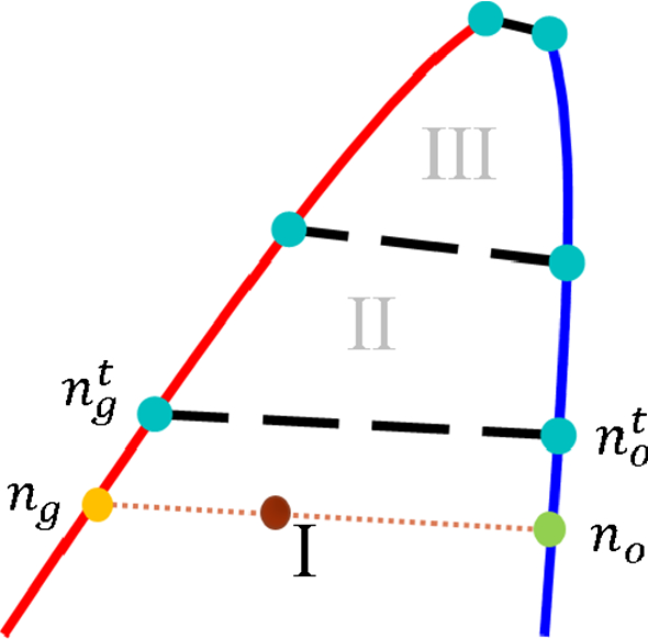

  

  Parameterization of the sub-region I of the compositional space

  Fig. 27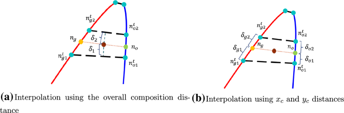

  

  Parameterization of sub-region II of the compositional space

• 3. Sub-region III between the last tie-line and the critical tie-line: this is sub-region III in Fig. 28. This sub-region witnesses the development of miscibility effects on relative-permeability. The length of tie-line is used as an interpolation parameter. Figure 28 shows the calculation of the relative-permeability parameters $n_{\mathrm{o}}$ and $n_{\mathrm{g}}$ using Eq. 15:

Fig. 28

Parameterization of the sub-region III of the compositional space

$$\begin{aligned} \begin{aligned} n_{\mathrm{g}}=\dfrac{l}{l_1^t}\times n_{\mathrm{g}}^t + \big (1-\dfrac{l}{l_1^t} \big )\times n_{\mathrm{g}}^{ct}\\ n_{\mathrm{o}}=\dfrac{l}{l_1^t}\times n_{\mathrm{o}}^t + \big (1-\dfrac{l}{l_1^t} \big )\times n_{\mathrm{o}}^{ct} \end{aligned} \end{aligned}$$

(15)

1.2 Additional Simulation Results

1.2.1 Four-Component Case

This case is based on Orr model (Orr 2007). For this run we use a mixture of $\text {CH}_{\mathrm{4}}$, $\text {C}_{\mathrm{2}}$H$_{6}$, $\text {NC}_{\mathrm{6}}$ and $\text {NC}_{\mathrm{16}}$ at pressure and temperature conditions of $p=137.9$ bar and $T=366.5$ K. We compare the two relative-permeability models CSP and STD. The compositional path for this case passes in the vicinity of the critical line. The endpoint relative-permeability for the oil and gas phases are $k_{ocw}$=0.5 and $k_{\mathrm{gcw}}=1$. The parameterization of the two-phase region uses a single tie-line at the edge $\text {CH}_{\mathrm{4}}$–$\text {NC}_{\mathrm{16}}$. Table 10 shows the compositional-pressure space parameterization for the CSP model.

Table 10 Single-hydrocarbon-phase relative-permeability parameterization

The compositional path for the models are different as it is shown in Fig. 29, this explains the difference in saturation of Fig. 30a and b (Tables 11 and 12).

Table 11 Four component case—performance comparison between compositional and standard Corey relative-permeability models for molar formulation

Table 12 Four component case—performance comparison between compositional and standard Corey relative-permeability models for natural formulation

For both formulations (Natural and Molar) the CSP model has less nonlinear iterations for all the cases we tested, the difference between the two models remains small as there is no discontinuities in phase labeling in this case compared to case 5.2, this can be reflected in the shape of the relative-permeability of Fig. 30b. We observe that the relative permeability is higher in the case of CSP for the grid cells where the composition is close to critical line, since the values of relative permeability for both phases converge to unity as we approach the critical line, a behavior that is not captured by the STD model (Figs. 31, 32).

Fig. 29

Four component case—compositional path at last time step

Fig. 30

Four component case, showing gas saturation, compositions and relative permeability at last time step

Fig. 31

Four component case—nonlinear performance for $dt=\{1, 5, 30\}$ using natural formulation

Fig. 32

Four component case—nonlinear performance for $dt=\{1, 5, 30\}$ using molar formulation

References

Alzayer, A.N.: Relative permeability of near-miscible fluids in compositional simulators. Master’s Thesis. Stanford University, pp. 1–157 (2015)
Alzayer, A.N., Voskov, D.V., Tchelepi, H.A.: Relative permeability of near-miscible fluids in compositional simulators. Transp. Porous Media (2017). https://doi.org/10.1007/s11242-017-0950-9
Aziz, K., Settari, A.: Petroleum Reservoir Simulation. Chapman and Hall, London (1979)
Beygi, M.R., et al.: Novel three-phase compositional relative permeability and three-phase hysteresis models. SPE J. 20(01), 21–34 (2015). https://doi.org/10.2118/165324-PA
Blunt, M.J.: An empirical model for three-phase relative permeability. SPE J. 5(4), 435–445 (2000). https://doi.org/10.2118/67950-pa
Christie, M.A., Blunt, M.J.: Tenth SPE comparative solution project: a comparison of upscaling techniques. SPE Reserv. Eval. Eng. 4(04), 308–317 (2001). https://doi.org/10.2118/72469-PA
Coats, K.H.: An equation of state compositional model. Soc. Pet. Engineers J. 20(05), 363–376 (1980). https://doi.org/10.2118/8284-PA. issn: 0197-7520
Dria, D.E., Pope, G.A., Sepehrnoori, K.: Three-phase gas/oil/brine relative permeabilities measured under CO2 flooding conditions. SPE Reserv. Eng. 80, 143–150 (1993)
Fayers, F.J. et al.: An improved three phase flow model incorporating compositional variance. In: SPE/DOE Improved Oil Recovery Symposium. Society of Petroleum Engineers (2000). https://doi.org/10.2118/59313-MS. ISBN: 978-1-55563-348-6
Iranshahr, A., Voskov, D.V., Tchelepi, H.A.: Gibbs energy analysis: compositional tie-simplex space. Fluid Phase Equilibria 321, 49–58 (2012). https://doi.org/10.1016/j.fluid.2012.02.001
Iranshahr, A., Voskov, D.V., Tchelepi, H.A.: A negative-flash tie-simplex approach for multiphase reservoir simulation. SPE J. 18(06), 1140–1149 (2013). https://doi.org/10.2118/141896-PA. issn: 1086-055X
Jerauld, G.R.: General three-phase relative permeability model for prudhoe bay. SPE Reserv. Eng. 12(4), 255–263 (1997). https://doi.org/10.2118/36178-PA
Khait, M., Voskov, D.V., Konidala, G.K.: Tie-simplex parametrization for operator-based linearization for non-isothermal multiphase compositional flow in porous (2018). https://doi.org/10.3997/2214-4609.201802183
Khorsandi, S., Li, L., Johns, R.T.: Equation of state for relative permeability, including hysteresis and wettability alteration. SPE J. 22, 1–915 (2017)
Li, C.C.: Critical temperature estimation for simple mixtures. Can. J. Chem. Eng. 49(5), 709–710 (1971). https://doi.org/10.1002/cjce.5450490529
Neshat, S., Pope, G.A.: Compositional three-phase relative permeability and capillary pressure models using gibbs free energy. In: SPE Reservoir Simulation Conference, p. 20 (2017). https://doi.org/10.2118/182592-MS
Oak, M.J., Baker, L.E., Thomas, D.C.: Three-phase relative permeability of berea sandstone. J. Pet. Technol. 42(8), 1054–1061 (1990). https://doi.org/10.2118/17370-pa
Orr, F.M.: Theory of Gas Injection Processes, p. 381. Tie-Line Publications, Copenhagen (2007). ISBN: 9788798996125
Petitfrere, M., De Loubens, R., Patacchini, L.: Continuous relative permeability model for compositional reservoir simulation, using the true critical point and accounting for miscibility. In: SPE Reservoir Simulation Conference (2019)
Prieditis, J., Wolle, C.R., Notz, P.K.: A laboratory and field injectivity study: CO2 WAG in the San Andres formation of West Texas. SPE (1991). https://doi.org/10.2523/22653-MS
Purswani, P., et al: On the development of a relative permeability equation of state, pp. 1–19 (2018). https://doi.org/10.3997/2214-4609.201802125. https://www.earthdoc.org/content/papers/10.3997/2214-4609.201802125
Shyeh-yung, J.J., Stadler, M.P.: Effect of injectant composition and pressure on displacement of oil by enriched hydrocarbon gases. SPE Reserv. Eng. 10, 109–115 (1995). https://doi.org/10.2118/28624-PA
Tang, D.E., Zick, A.A.: A new limited compositional reservoir simulator. In: SPE Symposium on Reservoir Simulation, p. 16 (1993). https://doi.org/10.2118/25255-MS
Voskov, D.V.: Operator-based linearization approach for modeling of multiphase multi-component flow in porous media. J. Comput. Phys. 337, 275–288 (2017)
Voskov, D.V., Tchelepi, H.A.: Tie-simplex based mathematical framework for thermodynamical equilibrium computation of mixtures with an arbitrary number of phases. Fluid Phase Equilibria 283(1–2), 1–11 (2009). https://doi.org/10.1016/j.fluid.2009.04.018
Voskov, D.V., Tchelepi, H.A.: Comparison of nonlinear formulations for two-phase multi-component EoS based simulation. J. Pet. Sci. Eng. 82–83, 101–111 (2012). https://doi.org/10.1016/j.petrol.2011.10.012
Voskov, D.V., Tchelepi, H.A., Younis, R.: General Nonlinear solution strategies for multiphase multicomponent EoS based simulation, p. 15 (2009). https://doi.org/10.2118/118996-MS
Whitson, C.H., Fevang, Ø.: Gas condensate relative permeability for well calculations. Transp. Porous Media (2003). https://doi.org/10.1023/A:1023539527573
Yuan, C., Pope, G.A.: A new method to model relative permeability in compositional simulators to avoid discontinuous changes caused by phase-identification problems. SPE J. 17(4), 1221–1230 (2012). https://doi.org/10.2118/142093-PA
Zaydullin, R., Voskov, D., Tchelepi, H.A.: Nonlinear formulation based on an equation-of-state free method for compositional flow simulation. SPE J. 18(02), 264–273 (2012). https://doi.org/10.2118/146989-PA
Zhou, Y., Tchelepi, H.A., Mallison, B.T.: Automatic differentiation framework for compositional simulation on unstructured grids with multi-point discretization schemes. In: SPE Reservoir Simulation Symposium (2011), p. 18. https://doi.org/10.2118/141592-MS
Zick, A.A.: Compositionally consistent models for relative permeability and capillary pressure. Tech. rep., pp. 1–76 (1989)
Acknowledgements
This research was funded by the Industrial Consortium on Reservoir Simulation Research at Stanford University (SUPRI-B). The authors would like to thank Birol Dindoruk for insightful discussions, and Huanquan Pan for help with flash application.
Funding
Funding was provided by the SUPRI-B research group within the Energy Resources Engineering Department of Stanford University.
Author information
Authors and Affiliations
Corresponding author
Ethics declarations
Conflict of interest
The authors declare that they have no known competing financial interests or personal relationships that could have appeared to influence the work reported in this paper.
Additional information
Publisher's Note
Springer Nature remains neutral with regard to jurisdictional claims in published maps and institutional affiliations.