Deformation theory of the blown-up Seiberg–Witten equation in dimension three

Abstract

Associated with every quaternionic representation of a compact, connected Lie group there is a Seiberg–Witten equation in dimension three. The moduli spaces of solutions to these equations are typically non-compact. We construct Kuranishi models around boundary points of a partially compactified moduli space. The Haydys correspondence identifies such boundary points with Fueter sections—solutions of a non-linear Dirac equation—of the bundle of hyperkähler quotients associated with the quaternionic representation. We discuss when such a Fueter section can be deformed to a solution of the Seiberg–Witten equation.

Appendices

A Examples of Seiberg–Witten equations

Example A.1

Let $G = \mathrm {U}(n)$ and $S = \mathbf {H}\otimes _{\mathbf {C}}{\mathbf {C}}^n$, where the complex structure on $\mathbf {H}$ is given by right-multiplication by i. Let $\rho : \mathrm {U}(n) \rightarrow \mathrm {Sp}(\mathbf {H}\otimes _{\mathbf {C}}{\mathbf {C}}^n)$ be induced from the standard representation of $\mathrm {U}(n)$. The corresponding Seiberg–Witten equation is the $\mathrm {U}(n)$–monopole equation in dimension three. The closely related ${\mathbf {P}\mathrm {U}}(2)$–monopole equation on 4–manifolds plays a crucial role in Pidstrigach and Tyurin’s approach to proving Witten’s conjecture relating Donaldson and Seiberg–Witten invariants; see, e.g., [8, 20, 27].

In this example as well as in Example 2.15, we have $\mu ^{-1}(0) = \lbrace 0 \rbrace$.

Example A.2

Let G be a compact Lie group, ${\mathfrak g}= {{\,\mathrm{Lie}\,}}(G)$, and fix an ${{\,\mathrm{Ad}\,}}$–invariant inner product on ${\mathfrak g}$. $S :=\mathbf {H}\otimes _\mathbf {R}{\mathfrak g}$ is a quaternionic Hermitian vector space, and $\rho : G \rightarrow \mathrm {Sp}(S)$ induced by the adjoint action is a quaternionic representation. The moment map $\mu : \mathbf {H}\otimes _\mathbf {R}{\mathfrak g}\rightarrow ({\text {Im}}\mathbf {H}\otimes {\mathfrak g})^*$ is given by

$$\begin{aligned} \mu (\xi )&= \frac{1}{2}[\xi ,\xi ] \\&= ([\xi _2,\xi _3]+[\xi _0,\xi _1])\otimes i + ([\xi _3,\xi _1]+[\xi _0,\xi _2])\otimes j + ([\xi _1,\xi _2]+[\xi _0,\xi _3])\otimes k \end{aligned}$$

for $\xi = \xi _0\otimes 1 + \xi _1\otimes i + \xi _2\otimes j + \xi _3\otimes k \in \mathbf {H}\otimes _\mathbf {R}{\mathfrak g}$. Set $H :=\mathrm {Sp}(1) \times G$ and extend the above quaternionic representation of G to H by declaring that $q \in \mathrm {Sp}(1)$ acts by right-multiplication with $q^*$.

Taking Q to be the product of the chosen spin structure ${\mathfrak s}$ with a principal G–bundle, and choosing B such that it induces the spin connection on ${\mathfrak s}$, (2.14) becomes

$$\begin{aligned} \mathrm{d}_A^*a&= 0, \\ *\mathrm{d}_Aa + \mathrm{d}_A\xi&= 0, \quad \text {and}\\ F_A&= \tfrac{1}{2}[a\wedge a] + *[\xi ,a]. \end{aligned}$$

for $\xi \in \Gamma ({\mathfrak g}_P)$, $a \in \Omega ^1(M,{\mathfrak g}_P)$ and $A \in \mathscr {A}(P)$. If M is closed, then integration by parts shows that every solution of this equation satisfies $\mathrm{d}_A\xi =0$ and $[\xi ,a]=0$; hence, $A + ia$ defines a flat $G^{\mathbf {C}}$–connection. Here $G^{\mathbf {C}}$ denotes the complexification of G.

In the above situation, we have $\mu ^{-1}(0)/G \cong (\mathbf {H}\otimes {\mathfrak t})/W$ where ${\mathfrak t}$ is a the Lie algebra of a maximal torus $T \subset G$ and $W = N_G(T)/T$ is the Weyl group of G. However, since each $\xi \in \mu ^{-1}(0)$ has stabilizer conjugate to T, we have $\mu ^{-1}(0)\cap S^\mathrm {reg}= \varnothing$, and the hyperkähler quotient $S^\mathrm {reg}{/\!\! /\!\! /}G$ is empty.

Example A.3

The motivating example for us is the (r, k) ADHM Seiberg–Witten equation, which we expect to play in important role in gauge theory on $G_2$–manifolds,⁸ and which arises from

$$\begin{aligned} S = {{\,\mathrm{Hom}\,}}_{\mathbf {C}}({\mathbf {C}}^r,\mathbf {H}\otimes _{\mathbf {C}}{\mathbf {C}}^k) \oplus \mathbf {H}^*\otimes _\mathbf {R}{\mathfrak u}(k) \end{aligned}$$

with

$$\begin{aligned} G = \mathrm {U}(k) \triangleleft H = \mathrm {SU}(r) \times \mathrm {Sp}(1) \times \mathrm {U}(k) \end{aligned}$$

where $\mathrm {SU}(r)$ acts on ${\mathbf {C}}^r$ in the obvious way, $\mathrm {U}(k)$ acts on ${\mathbf {C}}^k$ in the obvious way and on ${\mathfrak u}(k)$ by the adjoint representation, and $\mathrm {Sp}(1)$ acts on the first copy of $\mathbf {H}$ trivially and on the second copy by right-multiplication with the conjugate. Accoding to Atiyah, Drinfeld, Hitchin, and Manin [1], if $r \geqslant 2$, then $S^\mathrm {reg}{/\!\! /\!\! /}G$ is the moduli space of framed $\mathrm {SU}(r)$ ASD instantons of charge k on $\mathbf {R}^4$, and $\mu ^{-1}(0)/G$ is its Uhlenbeck compactification, If $r = 1$, then $\mu ^{-1}(0)\cap S^\mathrm {reg}= \varnothing$, and $\mu ^{-1}(0)/G = {{\,\mathrm{Sym}\,}}^k\mathbf {H}:=\mathbf {H}^k/S_k$ by [19, Example 3.14].

B Useful identities involving $\mu$

This appendix summarizes and proves a few useful identities regarding $\mu$, some of which are used in this article.

Proposition B.1

For $\xi \in \Omega ^0(M,{\mathfrak g}_P)$, $a \in \Omega ^1(M,{\mathfrak g}_P)$, and $\phi ,\psi \in \Gamma ({\mathfrak S})$, we have

$$\begin{aligned}{}[\xi ,\mu (\phi ,\psi )] = \mu (\phi ,\rho (\xi )\psi ) + \mu (\psi ,\rho (\xi )\phi ), \end{aligned}$$

(B.2)

and for $a \in \Omega ^1(M,{\mathfrak g}_P)$ and $\phi ,\psi \in \Gamma ({\mathfrak S})$, we have

$$\begin{aligned} 2[a \wedge \mu (\phi ,\psi )] = - * \rho ^*\left( ({\bar{\gamma }}(a)\phi )\psi ^*\right) - * \rho ^*\left( ({\bar{\gamma }}(a)\psi )\phi ^*\right) . \end{aligned}$$

(B.3)

Proof

For all $a \in \Omega ^1(M,{\mathfrak g}_P)$, we have

$$\begin{aligned} 2\langle [\xi ,\mu (\phi ,\psi ))], *a \rangle&= \langle \mu (\phi ,\psi ), -*[\xi ,a] \rangle \\&= \langle \phi , -{\bar{\gamma }}([\xi ,a])\psi \rangle \\&= -\langle \phi , \rho (\xi ){\bar{\gamma }}(a)\psi \rangle +\langle \phi , {\bar{\gamma }}(a)\rho (\xi )\psi \rangle \\&= \langle \rho (\xi )\phi , {\bar{\gamma }}(a)\psi \rangle +\langle \phi , {\bar{\gamma }}(a)\rho (\xi )\psi \rangle \\&= 2\langle \mu (\phi ,\rho (\xi )\psi ), *a \rangle +2\langle \mu (\psi ,\rho (\xi )\phi ), *a \rangle . \end{aligned}$$

This proves the first identity. To prove the second identity, note that, for all $\eta \in \Omega ^0(M,{\mathfrak g}_P)$, we have

$$\begin{aligned} 2\langle [a\wedge \mu (\phi ,\psi )], *\eta \rangle&= \langle 2\mu (\phi ), *[\eta ,a] \rangle \\&= \langle \phi , {\bar{\gamma }}([\eta ,a])\psi \rangle \\&= \langle \phi , \rho (\xi ){\bar{\gamma }}(a)\psi \rangle -\langle \phi , {\bar{\gamma }}(a)\rho (\xi )\psi \rangle \\&= -\langle \xi , \rho ^*\left( ({\bar{\gamma }}(a)\psi )\phi ^*\right) \rangle -\langle \xi , \rho ^*\left( ({\bar{\gamma }}(a)\phi )\psi ^*\right) \rangle . \end{aligned}$$

$\square$

Proposition B.4

For all $A \in \mathscr {A}(Q)$ and $\phi , \psi \in \Gamma ({\mathfrak S})$ we have

(B.5)

and

(B.6)

Proof

Fix a point $x \in M$, a positive local orthonormal frame $(e_i)$ around x with $(\nabla e_i)(x) = 0$, and let $\xi$ be a local section of ${\mathfrak g}_P$ defined in a neighborhood of x satisfying $(\nabla \xi )(x) = 0$. We set $\nabla ^A_i :=\nabla ^A_{e_i}$.

At the point $x \in M$, we compute with

This proves the first identity. To prove the second identity, we compute

$\square$

Proposition B.7

If $(\varepsilon ,\Phi ,A) \in (0,\infty )\times \Gamma ({\mathfrak S})\times \mathscr {A}_B(Q)$ is a solution of (2.21) and $R_\Phi (\xi ) = \rho (\xi )\Phi$, then

Here $(e_1,e_2,e_3)$ is local orthonormal frame, $(e^1,e^2,e^3)$ is the dual coframe, $F^B_{ij} :=F_B(e_i,e_j)$, $F^{\mathfrak s}_{ij} :=F_{\mathfrak s}(e_i,e_j)$ with $F_{\mathfrak s}$ denoting the curvature of the spin connection on ${\mathfrak s}$, and $e^{ij} :=e^i \wedge e^j$.

Proof

We compute

$$\begin{aligned} \mathrm{d}_A \rho ^*[(\nabla _A\Phi )\Phi ^*]&= \sum _{i,j=1}^3 \rho ^*[(\nabla ^A_i\nabla ^A_j\Phi )\Phi ^*] e^{ij} + \rho ^*[(\nabla ^A_j\Phi )(\nabla ^A_i\Phi )^*] e^{ij} \\&= \sum _{i,j=1}^3 \frac{1}{2}\rho ^*[(F^A_{ij} \cdot \Phi )\Phi ^*] e^{ij} + \rho ^*[(\nabla ^A_j\Phi )(\nabla ^A_i\Phi )^*] e^{ij}. \end{aligned}$$

Since

$$\begin{aligned} \sum _{i,j=1}^3 \rho ^*[\rho (\mu (\Phi )_{ij})\Phi )\Phi ] e^{ij} = R_\Phi ^*R_\Phi \mu (\Phi ), \end{aligned}$$

the result now follows from Proposition B.4. $\square$

C Proof of Proposition 3.2

For the reader’s convenience, we recall the definitions of the graded vector space $L^\bullet$,

$$\begin{aligned} L^0&:=\Omega ^0(M,{\mathfrak g}_P), \\ L^1&:=\Gamma ({\mathfrak S})\oplus \Omega ^1(M,{\mathfrak g}_P), \\ L^2&:=\Gamma ({\mathfrak S})\oplus \Omega ^2(M,{\mathfrak g}_P), \quad \text {and}\\ L^3&:=\Omega ^3(M,{\mathfrak g}_P), \end{aligned}$$

the graded Lie bracket $\llbracket \cdot ,\cdot \rrbracket$,

$$\begin{aligned} \llbracket a,b \rrbracket&:={[a\wedge b]}&\text {for } a,b \in \Omega ^\bullet (M,{\mathfrak g}_P), \\ \llbracket \xi ,\phi \rrbracket&:=\rho (\xi )\phi&\text {for } \xi \in \Omega ^0(M,{\mathfrak g}_P) \text { and } \phi \in \Gamma ({\mathfrak S}) \text { in degree }1\text { or }2, \\ \llbracket a,\phi \rrbracket&:=-{\bar{\gamma }}(a)\phi&\text {for } a \in \Omega ^1(M,{\mathfrak g}_P) \text { and } \phi \in \Gamma ({\mathfrak S}) \text { in degree }1, \\ \llbracket \phi ,\psi \rrbracket&:=-2\mu (\phi ,\psi )&\text {for } \phi , \psi \in \Gamma ({\mathfrak S}) \text { in degree }1,\text { and} \\ \llbracket \phi ,\psi \rrbracket&:=-*\rho ^*(\phi \psi ^*)&\text {for } \phi \in \Gamma ({\mathfrak S}) \text { in degree }1\text { and } \psi \in \Gamma ({\mathfrak S}) \text { in degree 2}, \end{aligned}$$

and the graded differential $\delta _{{\mathfrak c}}$,

We proceed in four steps.

Step 1$(L^\bullet ,\llbracket \cdot ,\cdot \rrbracket )$ is a graded Lie algebra.

We need to verify the graded Jacobi identity, that is, for every three homogeneous elements $x,y,z \in L^\bullet$ we need to show that

$$\begin{aligned} J(x,y,z) :=(-1)^{\deg {x}\cdot \deg {z}}\llbracket x,\llbracket y,z \rrbracket \rrbracket + (-1)^{\deg {y}\cdot \deg {x}}\llbracket y,\llbracket z,x \rrbracket \rrbracket + (-1)^{\deg {z}\cdot \deg {y}}\llbracket z,\llbracket x,y \rrbracket \rrbracket \end{aligned}$$

vanishes. Here $\deg {x}$ denotes the degree of x.

For degree reasons $J(x,y,z) = 0$, unless $\deg x + \deg y + \deg z \leqslant 3$. $(\Omega ^\bullet (M,{\mathfrak g}_P),{[\cdot \wedge \cdot ]})$ is a graded Lie algebra. Since J(x, y, z) is invariant under permutations of x, y, and z, we can assume that $z \in \Gamma ({\mathfrak S})$ in degree 1 or 2. Hence, only the following five cases remain:

• For $\xi ,\eta \in \Omega ^0(M,{\mathfrak g}_P)$, and $\phi \in \Gamma ({\mathfrak S})$ in degree 1 or 2, we have

  $$\begin{aligned} J(\xi ,\eta ,\phi )&= \llbracket \xi ,\llbracket \eta ,\phi \rrbracket \rrbracket + \llbracket \eta ,\llbracket \phi ,\xi \rrbracket \rrbracket + \llbracket \phi ,\llbracket \xi ,\eta \rrbracket \rrbracket \\&= \rho (\xi )\rho (\eta )\phi - \rho (\eta )\rho (\xi )\phi - \rho ([\xi ,\eta ])\phi = 0. \end{aligned}$$

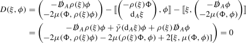
• For $\xi \in \Omega ^0(M,{\mathfrak g}_P)$, and $\phi ,\psi \in \Gamma ({\mathfrak S})$ in degree 1, we have

  $$\begin{aligned} J(\xi ,\phi ,\psi )&= \llbracket \xi ,\llbracket \phi ,\psi \rrbracket \rrbracket + \llbracket \phi ,\llbracket \psi ,\xi \rrbracket \rrbracket - \llbracket \psi ,\llbracket \xi ,\phi \rrbracket \rrbracket \\&= -2[\xi ,\mu (\phi ,\psi )] + 2\mu (\phi ,\rho (\xi )\psi ) + 2\mu (\psi ,\rho (\xi )\phi ) = 0 \end{aligned}$$

  by Proposition B.1.

• For $\xi \in \Omega ^0(M,{\mathfrak g}_P)$, $\phi \in \Gamma ({\mathfrak S})$ in degree 1 and $\psi \in \Gamma ({\mathfrak S})$ in degree 2, we have

  $$\begin{aligned} J(\xi ,\phi ,\psi )&= \llbracket \xi ,\llbracket \phi ,\psi \rrbracket \rrbracket + \llbracket \phi ,\llbracket \psi ,\xi \rrbracket \rrbracket + \llbracket \psi ,\llbracket \xi ,\phi \rrbracket \rrbracket \\&= -([\xi ,*\rho ^*\left( \phi \psi ^*\right) ] - *\rho ^*\left( \phi (\rho (\xi )\psi )^*\right) + *\rho ^*\left( \psi (\rho (\xi )\phi )^*\right) ) \\&= -*\rho ^*\left( [\rho (\xi ),\phi \psi ^*] + \phi \psi ^*\rho (\xi ) - \rho (\xi )\phi \psi ^*\right) = 0. \end{aligned}$$

• For $\xi \in \Omega ^0(M,{\mathfrak g}_P)$, $a \in \Omega ^1(M,{\mathfrak g}_P)$, and $\phi \in \Gamma ({\mathfrak S})$ in degree 1, we have

  $$\begin{aligned} J(\xi ,a,\phi )&= \llbracket \xi ,\llbracket a,\phi \rrbracket \rrbracket + \llbracket a,\llbracket \phi ,\xi \rrbracket \rrbracket - \llbracket \phi ,\llbracket \xi ,a \rrbracket \rrbracket ] \\&= -\rho (\xi ){\bar{\gamma }}(a)\phi + {\bar{\gamma }}(a)\rho (\xi )\phi + {\bar{\gamma }}({[\xi ,a]})\phi = 0. \end{aligned}$$

• For $a \in \Omega ^1(M,{\mathfrak g}_P)$ and $\phi ,\psi \in \Gamma ({\mathfrak S})$ in degree 1, we have

  $$\begin{aligned} J(a,\phi ,\psi )&= - \llbracket a,\llbracket \phi ,\psi \rrbracket \rrbracket - \llbracket \phi ,\llbracket \psi ,a \rrbracket \rrbracket - \llbracket \psi ,\llbracket a,\phi \rrbracket \rrbracket \\&= 2{[a\wedge \mu (\phi ,\psi )]} + *\rho ^*\left( ({\bar{\gamma }}(a)\psi )\phi ^*\right) + *\rho ^*\left( ({\bar{\gamma }}(a)\phi )\psi ^*\right) = 0 \end{aligned}$$

  by Proposition B.1.

Step 2$(L^\bullet ,\delta _{\mathfrak c}^\bullet )$ is a DGA.

We need to show that $\delta _{\mathfrak c}\circ \delta _{\mathfrak c}= 0$. Using Proposition B.1, we compute that

and, using Proposition B.4 and Proposition B.1, we compute that

Step 3$(L^\bullet ,\llbracket \cdot ,\cdot \rrbracket ,\delta _{\mathfrak c}^\bullet )$ is a DGLA.

We need to verify that $\delta _{\mathfrak c}^\bullet$ satisfies the graded Leibniz rule with respect to $\llbracket \cdot ,\cdot \rrbracket$, that is for every two homogeneous elements $x,y \in L^\bullet$ we need to show that

$$\begin{aligned} D(x,y) = \delta \llbracket x,y \rrbracket - \llbracket \delta x,y \rrbracket - (-1)^{\deg x}\llbracket x,\delta y \rrbracket \end{aligned}$$

vanishes.

For degree reasons, $D(x,y) = 0$ unless $\deg x + \deg y \leqslant 2$; hence, only the following eight cases remain:

• For $\xi ,\eta \in \Omega ^0(M,{\mathfrak g}_P)$, we have

  $$\begin{aligned} D(\xi ,\eta ) = \begin{pmatrix} -\rho ([\xi ,\eta ])\Phi \\ \mathrm{d}_A[\xi ,\eta ] \end{pmatrix} - \llbracket \begin{pmatrix} -\rho (\xi )\Phi \\ \mathrm{d}_A\xi \end{pmatrix} , \eta \rrbracket - \llbracket \xi , \begin{pmatrix} -\rho (\eta )\Phi \\ \mathrm{d}_A\eta \end{pmatrix} \rrbracket = 0. \end{aligned}$$

• For $\xi \in \Omega ^0(M,{\mathfrak g}_P)$ and $\phi \in \Gamma ({\mathfrak S})$ in degree 1, we have

  

  by Proposition B.1.

• For $\xi \in \Omega ^0(M,{\mathfrak g}_P)$ and $a \in \Omega ^1(M,{\mathfrak g}_P)$, we have

  $$\begin{aligned} D(\xi ,a)&= \begin{pmatrix} -{\bar{\gamma }}([\xi ,a])\Phi \\ \mathrm{d}_A [\xi ,a] \end{pmatrix} - \llbracket \begin{pmatrix} -\rho (\xi )\Phi \\ \mathrm{d}_A\xi \end{pmatrix} , a \rrbracket - \llbracket \xi , \begin{pmatrix} -{\bar{\gamma }}(a)\Phi \\ \mathrm{d}_A a \end{pmatrix} \rrbracket \\&= \begin{pmatrix} -{\bar{\gamma }}([\xi ,a])\Phi - {\bar{\gamma }}(a)\rho (\xi )\Phi + \rho (\xi ){\bar{\gamma }}(a)\Phi \\ \mathrm{d}_A [\xi ,a] - [\mathrm{d}_A\xi \wedge a] - [\xi ,\mathrm{d}_A] \end{pmatrix} = 0. \end{aligned}$$

• For $\xi \in \Omega ^0(M,{\mathfrak g}_P)$ and $\phi \in \Gamma ({\mathfrak S})$ in degree 2, we have

  $$\begin{aligned} D(\xi ,\phi )&= *\rho ^*(\rho (\xi )\phi \Phi ^*) - \llbracket \rho (\xi )\Phi ,\phi \rrbracket - \llbracket \mathrm{d}_A\xi ,\phi \rrbracket - \llbracket \xi , *\rho ^*(\phi \Phi ^*) \rrbracket \\&= *\rho ^*(\rho (\xi )\phi \Phi ^*) - * \rho ^*( \phi \Phi ^* \rho (\xi )) - [\xi ,*\rho ^*(\phi \Phi ^*)] = 0. \end{aligned}$$

• For $\xi \in \Omega ^0(M,{\mathfrak g}_P)$ and $b \in \Omega ^2(M,{\mathfrak g}_P)$, we have

  $$\begin{aligned} D(\xi ,b) = \mathrm{d}_A [\xi ,b] - [\mathrm{d}_A\xi ,b] - [\xi ,\mathrm{d}_Ab] = 0. \end{aligned}$$

• For $\phi ,\psi \in \Gamma ({\mathfrak S})$ in degree 1, we have

  

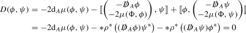
  by Proposition B.4.

• For $a \in \Omega ^1(M,{\mathfrak g}_P)$ and $\phi \in \Gamma ({\mathfrak S})$ in degree 1, we have

  

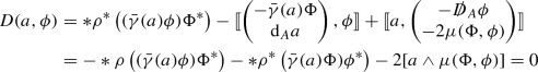
  by Proposition B.1.

• For $a,b \in \Omega ^1(M,{\mathfrak g}_P)$, we have

  $$\begin{aligned} D(a,b) = \begin{pmatrix} - {\bar{\gamma }}{ {[a\wedge b]}} \Phi \\ \mathrm{d}_A {[a\wedge b]} \end{pmatrix} - \llbracket \begin{pmatrix} {\bar{\gamma }}(a)\Phi \\ \mathrm{d}_A a \end{pmatrix} , b \rrbracket + \llbracket a , \begin{pmatrix} {\bar{\gamma }}(b)\Phi \\ \mathrm{d}_A b \end{pmatrix} \rrbracket = 0. \end{aligned}$$

Step 3 For every ${\hat{{\mathfrak c}}} :=(a,\phi ) \in L^1$, $(A+a,\Phi +\phi )$ solves (2.14) if and only if $\delta _{\mathfrak c}{\hat{{\mathfrak c}}} + \frac{1}{2}\llbracket {\hat{{\mathfrak c}}},{\hat{{\mathfrak c}}} \rrbracket = 0$.

For ${\hat{{\mathfrak c}}} :=(a,\phi ) \in L^1$, we have

which vanishes if and only if $(A+a,\Phi +a)$ solves (2.14). $\square$

References

Atiyah, M.F., Drinfeld, V.G., Hitchin, N.J., Manin, YuI: Construction of instantons. Phys. Lett. A 65(3), 185–187 (1978). https://doi.org/10.1016/0375-9601(78)90141-X
Atiyah, M.F., Patodi, V.K., Singer, I.M.: Spectral asymmetry and Riemannian geometry III. Math. Proc. Camb. Philos. Soc. 79(1), 71–99 (1976). https://doi.org/10.1017/S0305004100052105
Donaldson, S.K., Kronheimer, P.B.: The Geometry of Four-Manifolds. Oxford Mathematical Monographs, New York (1990)
Donaldson, S.K., Segal, E.P.: Gauge theory in higher dimensions, II. Surveys in differential geometry Volume XVI. Geom. Spec. Hol. Relat. Top. 16, 1–41 (2011)
Dancer, A., Swann, A.: The geometry of singular quaternionic Káhler quotients. Internat. J. Math. 8(5), 595–610 (1997). https://doi.org/10.1142/S0129167X97000317
Doan, A., Walpuski, T.: On the existence of harmonic Z2 spinors. J. Differ. Geom. (2018). arXiv:1710.06781 (to appear)
Doan, A., Walpuski, T.: On counting associative submanifolds and Seiberg-Witten monopoles. Pure Appl. Math. Q. 15(4), 1047–1133 (2019). https://doi.org/10.4310/PAMQ.2019.v15.n4.a4
Feehan, P. M. N., Leness, T. G.: PU(2) monopoles and relations between fourmanifold invariants. Topology and its Applications 88.1-2 (1998). Symplectic, contact and low-dimensional topology (Athens, GA, 1996), pp. 111–145 (1996). https://doi.org/10.1016/S0166-8641(97)00201-0
Guo, S., Wu, J.: Bifurcation theory of functional differential equations. Appl. Math. Sci. 184, x+289 (2013). https://doi.org/10.1007/978-1-4614-6992-6
Haydys, A.: Nonlinear Dirac operator and quaternionic analysis. Commun. Math. Phys. 281(1), 251–261 (2008). https://doi.org/10.1007/s00220-008-0445-1
Haydys, A.: Gauge theory, calibrated geometry and harmonic spinors. J. Lond. Math. Soc. 86(2), 482–498 (2012). https://doi.org/10.1112/jlms/jds008
Haydys, A.: Dirac operators in gauge theory. New ideas in low dimensional topology. (2014). arXiv:1303.2971
Haydys, A.: G2 instantons and the Seiberg-Witten monopoles. (2017). arXiv: 1703.06329
Hitchin, N.J., Karlhede, A., Lindström, U., Rocek, M.: Hyper-Kähler metrics and supersymmetry. Commun. Math.Phys. 108(4), 535–589 (1987). https://doi.org/10.1007/BF01214418
Haydys, A., Walpuski, T.: A compactness theorem for the Seiberg-Witten equation with multiple spinors in dimension three. Geom. Funct. Anal. 25(6), 1799–1821 (2015). https://doi.org/10.1007/s00039-015-0346-3
Kronheimer, P. B., Mrowka, T. S.: Monopoles and three-manifolds. Vol. 10. New Mathematical Monographs. (2007). https://doi.org/10.1017/CBO9780511543111.
Lim, Y.: A non-abelian Seiberg-Witten invariant for integral homology 3-spheres. Geom. Topol. 7, 965–999 (2003). https://doi.org/10.2140/gt.2003.7.965
Nakajima, H.: Towards a mathematical definition of Coulomb branches of 3-dimensional N = 4 gauge theories, I. Adv. Theor. Math. Phys. 20(3), 595–669 (2016). https://doi.org/10.4310/ATMP.2016.v20.n3.a4
Nakajima, H.: Lectures on Hilbert schemes of points on surfaces. Vol. 18. University Lecture Series (1999)
Pidstrigach, V. Ya, Tyurin, A.N.: Localisation of Donaldson invariants along the Seiberg-Witten classes. (1995). arXiv: dg-ga/9507004
Salamon, D.A.: The three-dimensional Fueter equation and divergence-free frames. Abhandlungen aus dem Mathematischen Seminar der Universität Hamburg 83(1), 1–28 (2013). https://doi.org/10.1007/s12188-013-0075-1
Strang, G.: Introduction to linear algebra. 5th edition, pp. x + 574 (2016)
Taubes, C.H.: PSL(2; C) connections on 3-manifolds with L2 bounds on curvature. Camb. J. Math. 1(2), 239–397 (2013). https://doi.org/10.4310/CJM.2013.v1.n2.a2
Taubes, C. H.: Compactness theorems for SL(2; C) generalizations of the 4-dimensional anti-self dual equations. (2013). arXiv: 1307.6447
Taubes, C. H.: On the behavior of sequences of solutions to U(1) Seiberg-Witten systems in dimension 4. (2016). arXiv: 1610.07163
Taubes, C.H.: Nonlinear generalizations of a 3-manifold’s Dirac operator. Trends in mathematical physics. AMS/IP Stud. Adv. Math. 13, 475–486 (1999)
Teleman, A.: Moduli spaces of PU(2)-monopoles. Asian J. Math. 4(2), 391–435 (2000). https://doi.org/10.4310/AJM.2000.v4.n2.a10
Walpuski, T.: Gauge Theory on G2-Manifolds. Imperial College London, London (2013)
Walpuski, T.: G2-instantons, associative submanifolds, and Fueter sections. Commun. Anal. Geom. 25(4), 847–893 (2017). https://doi.org/10.4310/CAG.2017.v25.n4.a4
Walpuski, T.: A compactness theorem for Fueter sections. Comm. Math. Helvetici 92(4), 751–776 (2017). https://doi.org/10.4171/CMH/423
Acknowledgements
This material is based upon work supported by the National Science Foundation under Grant No. 1754967 and the Simons Collaboration “Special Holonomy in Geometry, Analysis and Physics”.
Author information
Authors and Affiliations
Corresponding author
Additional information
Publisher's Note
Springer Nature remains neutral with regard to jurisdictional claims in published maps and institutional affiliations.