Monthly Precipitation Forecasts Using Wavelet Neural Networks Models in a Semiarid Environment

Abstract

Accurate forecast of hydrological data such as precipitation is critical in order to provide useful information for water resources management, playing a key role in different sectors. Traditional forecasting methods present many limitations due to the high-stochastic property of precipitation and its strong variability in time and space: not identifying non-linear dynamics or not solving the instability of local weather situations. In this work, several alternative models based on the combination of wavelet analysis (multiscalar decomposition) with artificial neural networks have been developed and evaluated at sixteen locations in Southern Spain (semiarid region of Andalusia), representative of different climatic and geographical conditions. Based on the capability of wavelets to describe non-linear signals, ten wavelet neural network models (WNN) have been applied to predict monthly precipitation by using short-term thermo-pluviometric time series. Overall, the forecasting results show differences between the ten models, although an effective performance (i.e., correlation coefficients ranged from 0.76 to 0.90 and Root Mean Square Error values ranged from 6.79 to 29.82 mm) was obtained at each of the locations assessed. The most appropriate input variables to obtain the best forecasts are analyzed, according to the geo-climatic characteristics of the sixteen sites studied.

1. Introduction

Precipitation, besides being one of the most important variables in hydrological models (infiltration, soil loss, droughts, overland flow production, floods, etc.), is crucial in sectors such as agriculture, tourism or even in the energy sector [1], where the absence of water can lead to the closure of nuclear plants, such as the recent case in July 2019 in France. Therefore, the improvement of precipitation predictions is one of the greatest current challenges of the scientific community. Likewise, accurate precipitation forecasting is a very difficult and relevant mechanism of the hydrologic cycle due to its high spatial-temporal variability. Because of the large number of interconnected variables that are involved in the physical modelling of precipitation, forecasting rainfall is exceptionally complicated [2]. Due to the nonlinear and dynamic characteristics of precipitation, methods like numerical weather prediction (NWP) models or even statistical models still have difficulties to provide satisfactory precipitation forecasts [3]. This is mainly due to the fact that they are subject to many uncertainties [4,5,6,7,8,9] such as not solving the local weather situations or not identifying non-linear dynamics in time-series, among others [10,11,12].

In this sense, the mathematical models called Artificial Neural Networks (ANN), which are inspired by how the human nervous system works, have many strengths. One of them, which is highly important, is their ability to learn from experience. ANN models are based on a set of processing elements called neurons and they can accumulate a large amount of behaviors, allowing users to forecast previously nonexistent patterns. Another advantage is that neurons in ANNs work in a parallel processing mechanism, being able to process—as singular or multi-layered information—big data efficiently. Lastly, they can extract complex nonlinear relationships between variables, which can be very useful for precipitation modeling. The concept of artificial neurons was introduced by the authors in [13] but the ANN applications have increased since the back-propagation learning method was developed [14]. Since then, the use of ANN in the field of research has turned into a multitude of satisfactory solutions to problems that are not easily solved with traditional techniques, especially when the quality is doubtful and the quantity is scarce [15]. One of the most used ANN architectures is the so-called feed-forward multilayer perceptron (FFMLP), where all the information propagates in one direction toward the output layer with no feedback. This architecture is explained in detail in Section 2.2. In addition, their use is very advantageous, of great versatility and easy handling because these models do not need to formulate the mathematical description of the complex mechanisms involved in the process.

In hydrological modeling, the Artificial Neural Network techniques were applied for the first time by [16]. Since then, numerous works successfully address improvements in models of rainfall-runoff [17,18,19], stream-flow [20,21,22], water quality [15,23,24], ground water [25,26] and even for data validation as a quality assurance procedure [27,28]. In 2000, the American Society of Civil Engineering published two technical works related to Hydrology and ANNs [29,30] whose results have been discussed in depth and compared to other modelling techniques. Recently, a work summarizing a review of neural networks techniques applied to hydrological systems has been reported [31].

In relation to works that exclusively deal with the forecast of precipitation time series using ANN, several studies can be found in the scientific literature. An ANN model for precipitation forecasting in Thailand was developed by [32] using various meteorological parameters measured at surrounding stations. In some regions of Greece, researchers [33] obtained precipitation predictions using ANNs and 115-years datasets. Others works such as [34] and [35], used various climate indices (North Atlantic Oscillation -NAO-, Southern Oscillation -SOI-, etc.) as input variables in Korea and Australia, respectively. In China, several works based on ANNs have been developed using long-term historical datasets [3,36,37]. Moreover, similar models have been applied in different Indian regions [38,39,40,41]. Some of the main problems of this kind of models are the non-availability of historical records at many locations, the non-existence of neighboring stations and the impossibility of arranging the previously mentioned climate indices (NAO, SOI, etc.) in near-real time in order to forecast one-step ahead.

1.1. Wavelet Multiscale Analysis

The multiscalar characterization of precipitation has been studied for several years in different regions of the world using various approaches and for different purposes [42,43,44,45,46,47]. Especially in the current context of climate variability and change, all the techniques that are capable of deepening the stochastic behavior of precipitation time series are of great interest for use in many applications [48]. One of the most effective is the wavelet analysis [49], because it can provide an exact location of any changes in the dynamic patterns of the time series, being widely applied in hydrological topics such as forecasting [50,51,52], rainfall trends [53] or water quality modelling [54], among others. Wavelets are a class of functions that cut up data into different frequency components and they are used to localize a given function in both position and scaling. A wavelet transformation is a powerful mathematical signal processing tool, able to produce both time and frequency information and providing multiresolution analysis. There are two main types of wavelet transforms: continuous and discrete, being the most extensively used. The main advantage of wavelets versus Fourier analysis is its power to process non-stationarity signals, determining the temporal variation of the frequency content and allowing users to track the evolution of processes at different timescales in data sequences.

Different wavelet families have been studied for different purposes depending on the time series to be analyzed: Coiflets, Symlets, Daubechies, Feyer-Korovkin, BiorSplines, among others. In hydrologic modelling, Daubechies wavelet [55] is one of the most employed due to its orthonormality properties and its good trade-off between parsimony and information plenitude [56,57,58]. This kind of wavelet has associated subclasses (db1 or haar, db2, db3, …dbN) depending on the number of vanishing moments and there is a scaling function generating an orthogonal multi-resolution analysis. This multiple-level decomposition process estimates the discrete wavelet transform coefficients, breaking down the original time-series into several lower-resolution components as a set of sub-signals: approximation (cAN) and details (cDN). For example, for level of decomposition = 2 this iterative process will lead to cA2, cD1, cD2 sub-series. The approximation coefficients were produced by low-pass filter and details coefficients by high-pass filter, representing the low and high frequency components, respectively. Figure 1 shows the multiresolution analysis based on this wavelet decomposition. Thus, these meteorological sub-series generated by wavelet transformation can be used as input variables in ANN approaches, giving rise to a type of so-called hybrid models: Wavelet Neural Networks (WNN).

1.2. Availability of Short-Term Meteorological Series

Precipitation, and also temperature, are meteorological variables widely measured worldwide in comparison to solar radiation, humidity or wind speed, among others [59,60,61,62]. Besides, their behavior within the climate system is being studied all over the world [63], as both variables represent the key controlling factors in the spatial variation of terrestrial ecosystem carbon exchange [64]. However, long-term series are not easily available and often contain many gaps and have undergone homogenization or filling-gap processes usually due to changes in location, sensor replacement, variations in the mechanisms of data collection and measurements, etc.

In order to improve the weather monitoring systems among other aims, the installation of automated weather stations networks able to collect at least temperature and precipitation data has been increasing since the ending of past century practically worldwide [65] and more recently with the combination of low-cost sensors and Internet of Things devices [66]. Therefore, there is currently a large availability of thermo-precipitation records from numerous spatially distributed locations with almost entirely no gaps and with more than a decade in length. Thus, and due to many recent works reporting the improvement of ANN-based hydrological models combining them with wavelet analysis [3,67,68,69,70], the main goal of this work is the development and assessment of different hybrid WNN models to accurately forecast monthly precipitation in the semiarid and heterogeneous region of Andalusia (Southern Spain) using only short-term thermo-precipitation validated datasets. Due to the importance of precipitation forecast and since the availability of these data will increase in the coming years, the present work may be extensible to many other climatic areas of the world where these records are collected. Moreover, this work evaluates the use of new input thermal variables, in addition to precipitation, to deepen the knowledge and analyze the effectiveness of these hybrid models to forecast monthly precipitation in a geo-climatic variety of locations that have very different precipitation patterns.

For these purposes, different stations in the semiarid region of Andalusia (Southern Spain) were selected. Wavelet decompositions were applied to initial datasets in order to generate the input variables of the neural network models. The performance of all the WNN approaches has been evaluated using different statistics at each location.

2. Materials and Methods

2.1. Source of Data

Datasets used in this work were obtained from the Agroclimatic Information Network of Andalusia and they are easily downloadable on a daily basis from http://www.juntadeandalucia.es/agriculturaypesca/ifapa/ria/ (access on 2 August 2019), where there are some automated weather stations recently installed and others not operational. Andalusia is a semiarid region located in the South of the Iberian Peninsula (South-western Europe) covering almost 88,000 km² and is divided into eight provinces: Almería, Cádiz, Córdoba, Granada, Huelva, Jaén, Málaga and Sevilla. According to its relief it is a very heterogeneous region: from the extensive coastal plains of the Guadalquivir River (at sea level) to the highest areas of the Iberian Peninsula (‘Sierra Nevada’ in the province of Granada). In terms of dryness, high contrasts are found from the Tabernas desert (province of Almería) to the rainiest areas of Spain in the ‘Sierra de Grazalema’ Natural Park (province of Cádiz). Another singularity is that it is surrounded by the Mediterranean Sea and the Atlantic Ocean at its Southeast and Southwest sides, respectively. The geographical distribution of the stations used in this work is shown in Figure 2 and

Table 1. Name of the station, province, coordinates, elevation and data time-period of the weather stations used in this study (Southern Spain).

Station Name	Province	Latitude (°)	Longitude (°)	Elevation (m)	Time Period (Calibration) Time Period (Validation)
Tabernas (ALM04)	Almería	37.0925 N	2.3011 W	435	March 2000–August 2016 September 2016–July 2019
Huércal Overa (ALM07)	Almería	37.4133 N	1.8831 W	317	February 2000–August 2016 September 2016–July 2019
Conil Frontera (CAD05)	Cádiz	36.3372 N	6.1306 W	26	November 2000–November 2016 December 2016–July 2019
Jimena Frontera (CAD07)	Cádiz	36.4136 N	5.3844 W	53	January 2001–September 2016 October 2016–July 2019
El Carpio (COR05)	Córdoba	37.9150 N	4.5025 W	165	December 2000–September 2016 November 2016–July 2019
Santaella (COR07)	Córdoba	37.5236 N	4.8842 W	207	November 2000–November 2016 December 2016–July 2019
Loja (GRA03)	Granada	37.1706 N	4.1369 W	487	October 2000–September 2016 October 2016–July 2019
Cádiar (GRA07)	Granada	36.9242 N	3.1825 W	950	October 2000–September 2016 October 2016–July 2019
Puebla Guzmán (HUE07)	Huelva	37.5533 N	7.2469 W	288	December 2000–September 2016 November 2016–July 2019
El Campillo (HUE08)	Huelva	37.6622 N	6.5981 W	406	December 2000–September 2016 November 2016–July 2019
Mancha Real (JAE04)	Jaén	37.9175 N	3.5950 W	436	October 2000–September 2016 October 2016–July 2019
Sabiote (JAE07)	Jaén	38.0806 N	3.2342 W	822	October 2000–September 2016 October 2016–July 2019
Málaga (MAG01)	Málaga	36.7575 N	4.5364 W	68	November 2000–November 2016 December 2016–July 2019
Cártama (MAG09)	Málaga	36.7181 N	4.6769 W	95	August 2001–October 2016 November 2016–July 2019
Écija (SEV07)	Sevilla	37.5942 N	5.0756 W	125	December 2000–September 2016 November 2016–July 2019
IFAPA Las Torres-Tomejil (SEV101)	Sevilla	37.4008 N	5.5875 W	75	November 2001–November 2016 December 2016–July 2019

reports some of their characteristics, with latitudes ranging from 36.3372° to 38.0806° N, longitudes from 1.8831° to 7.2469° W and site elevations from 26 to 822 m above mean sea level. In general, the aridity increases from East (Huelva province) to West (Almería province) across Andalusia region [71]. These sites were selected in order to represent this climatic variability of the region, including coastal (‘Málaga’ and ‘Conil de la Frontera’ stations) and inland locations, and ensuring that the available time series are complete and gap-free.

Time-periods of monthly precipitation, maximum and minimum temperature datasets from each station are summarized in Table 1. All of them end in July 2019 and start in 2000/2001, ranging from 213 months at ‘IFAPA las Torres-Tomejil’ station to 234 months at ‘Huércal-Overa’ station. In order to assess model performances and following the method previously described [54], the first 85% of datasets was used to calibrate the models and the remaining 15% of the records was used for validation (at least two and a half years at all locations).

Table 2. Statistics of monthly precipitation, maximum and minimum temperature (Std: Standard Deviation; Max: Maximum; Min: Minimum).

Sites	Datasets	Precipitation (mm)				Maximum Temperature (°)				Minimum Temperature (°)
		Mean	Std	Max	Min	Mean	Std	Max	Min	Mean	Std	Max	Min
Tabernas (ALM04)	All	19.95	25.56	141.40	0.00	29.85	6.59	42.55	15.53	4.69	6.40	17.18	−8.20
	Validation	18.77	27.25	141.40	0.00	29.13	6.49	41.70	17.68	4.44	6.09	15.10	−5.30
	Calibration	20.17	25.30	128.40	0.00	29.98	6.62	42.55	15.53	4.74	6.47	17.18	−8.20
Huércal-Overa (ALM07)	All	22.49	31.94	247.80	0.00	29.89	6.02	43.58	17.03	4.54	6.46	17.18	−8.85
	Validation	19.57	34.37	186.80	0.00	29.90	5.87	40.76	18.57	4.37	6.12	15.19	−6.00
	Calibration	23.02	31.55	247.80	0.00	29.88	6.06	43.58	17.03	4.58	6.53	17.18	−8.85
Conil de la Frontera (CAD05)	All	42.71	54.32	287.60	0.00	28.72	6.45	41.37	16.04	6.53	5.02	15.80	−5.38
	Validation	37.95	55.09	208.60	0.00	28.00	6.80	40.30	18.96	5.91	4.72	15.80	−1.03
	Calibration	43.58	54.28	287.60	0.00	28.86	6.39	41.37	16.04	6.65	5.07	15.37	−5.38
Jimena de la Frontera (CAD07)	All	61.05	75.03	441.00	0.00	30.18	6.74	46.57	18.64	5.99	5.26	16.02	−3.88
	Validation	63.22	86.12	371.40	0.00	29.86	5.90	42.28	19.62	5.73	5.05	14.70	−1.51
	Calibration	60.66	73.11	441.00	0.00	30.23	6.89	46.57	18.64	6.04	5.31	16.02	−3.88
El Carpio (COR05)	All	41.23	48.84	317.60	0.00	31.38	8.59	47.10	15.42	4.89	6.58	17.93	−9.54
	Validation	38.12	48.55	260.20	0.00	31.54	8.56	47.10	19.61	4.32	6.50	15.40	−6.15
	Calibration	41.78	48.99	317.60	0.00	31.35	8.61	46.94	15.42	4.99	6.60	17.93	−9.54
Santaella (COR07)	All	44.27	50.85	310.80	0.00	30.64	8.15	45.69	17.36	6.08	6.05	17.27	−8.25
	Validation	42.47	54.85	277.80	0.00	29.96	7.94	44.91	18.69	6.21	5.64	16.10	−3.05
	Calibration	44.60	50.25	310.80	0.00	30.76	8.20	45.69	17.36	6.06	6.14	17.27	−8.25
Loja (GRA03)	All	36.96	39.12	230.60	0.00	29.87	7.53	45.94	16.92	4.05	6.01	15.37	−9.45
	Validation	35.66	44.21	225.40	0.00	29.97	7.90	45.94	16.92	4.08	5.94	14.70	−5.80
	Calibration	37.20	38.25	230.60	0.00	29.86	7.48	42.85	17.08	4.05	6.04	15.37	−9.45
Cádiar (GRA07)	All	43.46	56.88	423.60	0.00	27.11	7.02	42.63	14.17	5.03	6.06	18.38	−13.30
	Validation	42.55	61.55	317.00	0.00	26.26	7.03	41.20	16.11	4.43	6.37	15.90	−13.30
	Calibration	43.62	56.18	423.60	0.00	27.26	7.03	42.63	14.17	5.14	6.02	18.38	−8.13
Puebla Guzmán (HUE07)	All	46.69	53.29	296.80	0.00	29.21	7.84	43.63	15.42	6.60	5.09	16.38	−4.02
	Validation	43.36	50.38	197.80	0.00	29.24	7.62	42.18	18.65	6.82	4.68	15.50	−0.73
	Calibration	47.29	53.90	296.80	0.00	29.21	7.89	43.63	15.42	6.56	5.17	16.38	−4.02
El Campillo (HUE08)	All	60.51	69.67	389.80	0.00	29.51	7.63	43.07	15.41	6.95	4.81	16.39	−2.39
	Validation	56.16	66.43	351.00	0.00	29.48	7.61	42.74	18.92	6.78	4.58	15.40	−1.37
	Calibration	61.28	70.38	389.80	0.00	29.51	7.65	43.07	15.41	6.98	4.86	16.39	−2.39
Mancha Real (JAE04)	All	37.28	38.43	248.20	0.00	27.79	7.96	41.91	13.40	5.02	6.30	18.08	−10.24
	Validation	32.12	38.83	200.20	0.00	27.97	8.30	41.91	14.75	4.67	5.92	16.70	−6.62
	Calibration	38.22	38.38	248.20	0.00	27.76	7.92	41.62	13.40	5.09	6.38	18.08	−10.24
Sabiote (JAE07)	All	32.65	33.43	192.00	0.00	30.36	8.20	45.25	15.84	6.08	6.77	19.96	−8.64
	Validation	28.96	36.93	192.00	0.00	30.18	8.51	45.25	17.60	5.92	6.44	18.20	−5.06
	Calibration	33.32	32.81	174.20	0.00	30.39	8.16	44.23	15.84	6.11	6.85	19.96	−8.64
Málaga (MAG01)	All	38.10	50.99	272.70	0.00	30.09	6.38	42.78	18.44	7.66	5.92	19.10	−4.27
	Validation	38.18	54.26	199.40	0.00	29.60	5.88	39.60	21.14	7.28	5.35	19.10	−0.85
	Calibration	38.09	50.53	272.70	0.00	30.17	6.47	42.78	18.44	7.73	6.03	18.75	−4.27
Cártama (MAG09)	All	39.77	54.17	266.00	0.00	30.69	6.46	43.13	18.92	7.08	5.66	17.73	−2.60
	Validation	36.60	50.64	177.40	0.00	30.31	6.38	40.48	21.30	6.58	5.58	17.20	−1.38
	Calibration	40.33	54.89	266.00	0.00	30.76	6.49	43.13	18.92	7.17	5.69	17.73	−2.60
Écija (SEV07)	All	40.40	48.05	292.40	0.00	31.33	8.31	46.05	16.77	5.54	6.39	18.20	−9.09
	Validation	38.42	45.95	217.20	0.00	31.06	8.29	46.05	19.61	5.28	6.11	16.20	−3.78
	Calibration	40.76	48.52	292.40	0.00	31.38	8.34	45.96	16.77	5.59	6.45	18.20	−9.09
IFAPA C. Torres-T (SEV101)	All	41.46	48.12	282.00	0.00	31.42	8.16	53.12	18.05	5.43	6.11	16.72	−9.82
	Validation	37.10	46.22	203.40	0.00	30.85	8.31	44.85	18.88	5.16	5.83	16.10	−3.99
	Calibration	42.25	48.54	282.00	0.00	31.52	8.15	53.12	18.05	5.48	6.17	16.72	−9.82

shows the statistical values of these datasets for monthly precipitation, maximum and minimum temperature for each location.

In order to ensure reliability of datasets, a set of checking quality procedures has been applied to precipitation and temperature daily data following the guidelines proposed by [72]. In addition, a specific algorithm for detecting spurious precipitation signals [73] and the spatial regression test [74] were also carried out. The application of these quality assurance techniques to hydro-meteorological data have been successfully carried out under different climatic conditions worldwide as a pre-requisite before their use [75,76,77,78].

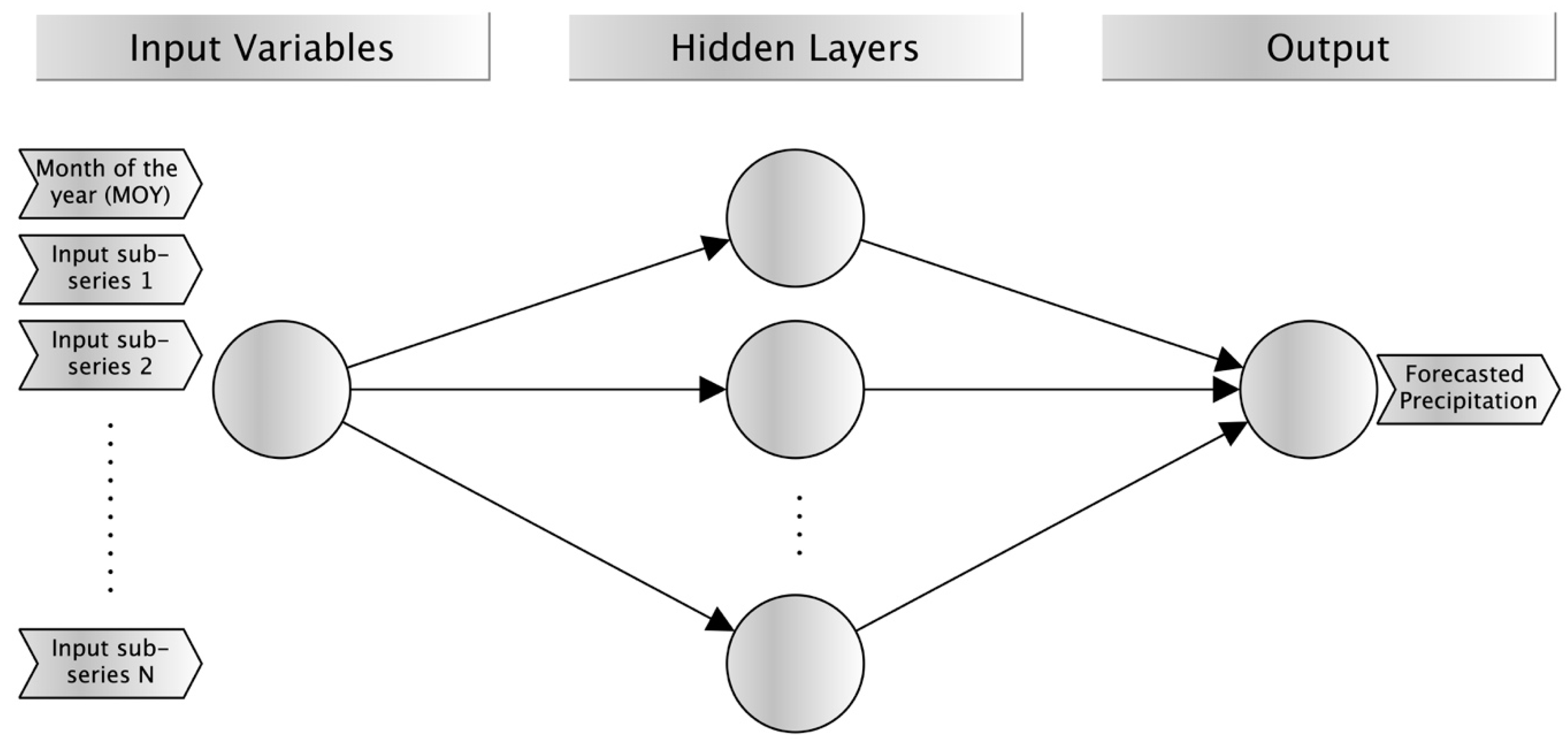
2.2. Development of Wavelet Neural Network (WNN) Models

Several hybrid models (WNN) were developed based on the use of the sub-series resulting from the wavelet decomposition of the original series, as input variables of a feed-forward multilayer perceptron neural network (FFMLP). This architecture (Figure 3) is the most widely-used in water resources modelling [79] and consists of an input layer, one or more hidden layers containing network computation nodes (neurons), and the output layer that contains the target variable (predicted precipitation). The number of input nodes is equal to the number of input variables (details and approximations of sub-time series and month of year) and the number of hidden nodes is determined by trial and error procedure. One of the main keys for the good behavior of these approaches is the ability to learn from experience using the well-known backpropagation method in the training process and optimized by applying the Levenberg–Marquardt algorithm. Eventually, logarithmic sigmoidal and pure linear transfer activation functions were used for the hidden and output layers, respectively, converting input signals into output signals. Thus, the process that takes place in the neurons is the following. Firstly, the inputs are multiplied by their corresponding initial weights; these products with a bias term are summed. Afterwards, this result passes as the input of an activation function which determines whether the neuron is activated or not. Then, the result advances to the next neurons and the process is repeated until the output is obtained (it is mathematically expressed as Equation (1)). Finally, the backpropagation training method consists of modifying the weights of the nodes based on the minimization of the bias errors (difference between target and output value) and all the process is repeated from the beginning.

$$O=\varnothing \left(\sum WI-\theta \right)$$

(1)

where O = output value of the hidden/output node, I = input or hidden node value, $\varnothing$ = the transfer function, W = weights connecting nodes and $\theta$ = bias for each node.

The selection of the Daubechies wavelet of order 5 (db5) was performed after a trial and error procedure checking Daubechies wavelet from order 1 to 10 [68,80,81], although similar results were found with db9. The wavelet decomposition process was carried out according to the procedure in [82] at level 3, based on the size of validation datasets for testing the model performances [69]. Finally, the optimal number of neurons in the hidden layer [2,68,83] was set to eight, after testing from two to ten in steps of one and checking the FFMLP performance.

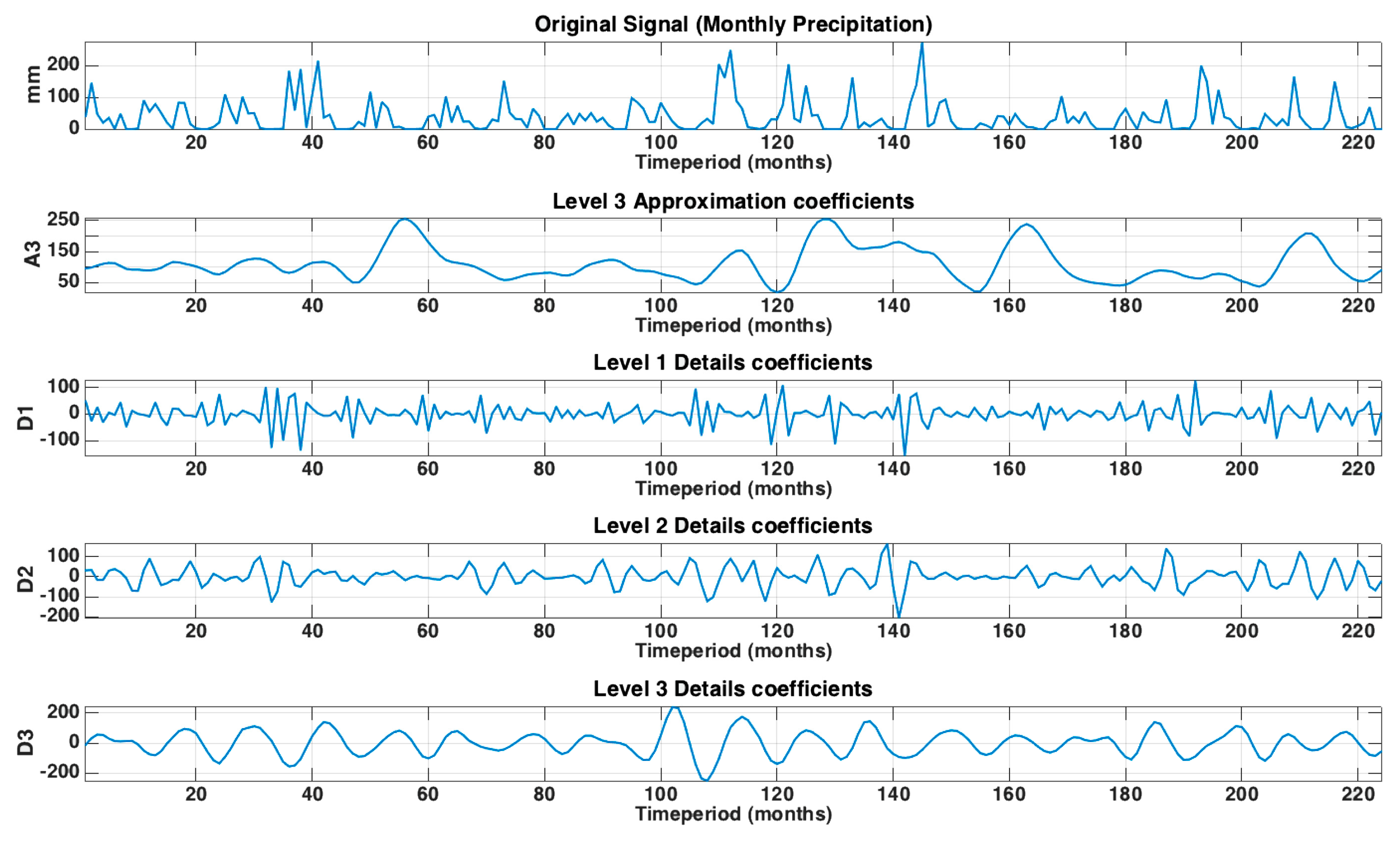
Thus, each dataset was decomposed by wavelet transformation into sub-series containing approximation coefficients (cA3) and details coefficients (cD1, cD2 and cD3). They were used as input variables for the WNN models as well as the month of year (MOY: 1 = January, 2 = February…12 = December), and monthly precipitation original series was used as the target output values. An example of the sub-series of precipitation (details and approximations) after the wavelet decomposition as well as the original signal is represented in Figure 4 for Málaga station.

The input variables used in each model are summarized in

Table 3. Inputs and number of variables of each of the wavelet neural network models (WNN) models evaluated in this work (m = month; MOY = month of year; P = precipitation; DTR_m = mean diurnal temperature range; DTR_x = maximum diurnal temperature range; DTR_n = minimum diurnal temperature range; MTR=monthly temperature range; T_x=maximum temperature; T_n = minimum temperature).

Models	Output	Input Variables	Nº Variables
I	P (m + 1)	MOY, P{decomposed} (m)	5
II	P (m + 1)	MOY, P{decomposed} (m), P{decomposed} (m−1)	9
III	P (m + 1)	MOY, P{decomposed} (m), DTRm {decomposed} (m)	9
IV	P (m + 1)	MOY, P{decomposed} (m), DTRx {decomposed} (m)	9
V	P (m + 1)	MOY, P{decomposed} (m), DTRn {decomposed} (m)	9
VI	P (m + 1)	MOY, P{decomposed} (m), DTRx {decomposed} (m), DTRn {decomposed} (m)	13
VII	P (m + 1)	MOY, P{decomposed} (m), MTR {decomposed} (m)	9
VIII	P (m + 1)	MOY, P{decomposed} (m), Tx{decomposed} (m)	9
IX	P (m + 1)	MOY, P{decomposed} (m), Tn{decomposed} (m)	9
X	P (m + 1)	MOY, P{decomposed} (m), Tx{decomposed}, Tn{decomposed} (m)	13

. All the models used Month of year (MOY) and precipitation signal decomposed by wavelets transformation. The proposed models used different combination of variables. For instance, the input variables of the Model I were MOY and monthly precipitation signal (decomposed into D1, D2, D3 and A3 coefficients). In contrast, the Model IX used MOY, precipitation signal (decomposed into D1, D2, D3 and A3 coefficients) and monthly minimum temperature signal (decomposed into D1, D2, D3 and A3 coefficients).

2.3. Statistical Analysis and Performance Criteria

In order to evaluate the performance of different models developed in this work, forecasted and measured precipitation values were compared by using simple error analysis. Thus, common statistical indices widely used to assess hydro-meteorological prediction models [26,61,68] were estimated: RMSE (root mean square error), R (Correlation Coefficient), MAPE (mean absolute percentage error) and NSE (Nash–Sutcliffe model efficiency coefficient, also known as coefficient of efficiency). These statistics are summarized from Equations (2) to (5):

$$RMSE=\sqrt{\frac{{{\displaystyle \sum }}_{t=1}^N\left(P_t^m-P_t^f\right)}{N}}$$

(2)

$$R=\frac{{{\displaystyle \sum }}_{t=1}^N\left(P_t^m-\overline{P^m}\right)\left(P_t^f-\overline{P^f}\right)}{\sqrt{\left[{{\displaystyle \sum }}_{t=1}^N{\left(P_t^m-\overline{P^m}\right)}^2\right]\left[{{\displaystyle \sum }}_{t=1}^N{\left(P_t^f-\overline{P^f}\right)}^2\right]}}$$

(3)

$$MAPE=\frac{100\%}{N}{\displaystyle \sum }_{t=1}^N\left|\frac{P_t^m-P_t^f}{P_t^m}\right|$$

(4)

$$NSE=1-\frac{{{\displaystyle \sum }}_{t=1}^N{\left(P_t^m-P_t^f\right)}^2}{{{\displaystyle \sum }}_{t=1}^N{\left(P_t^m-\overline{P^m}\right)}^2}$$

(5)

where the N is the number of months and $P_t^m$,$P_t^f$,$\overline{P^m}$ and$\overline{P^f}$ are precipitation measured at month t, precipitation forecasted at month t, the mean of measured monthly precipitation and the mean of forecasted monthly precipitation, respectively.

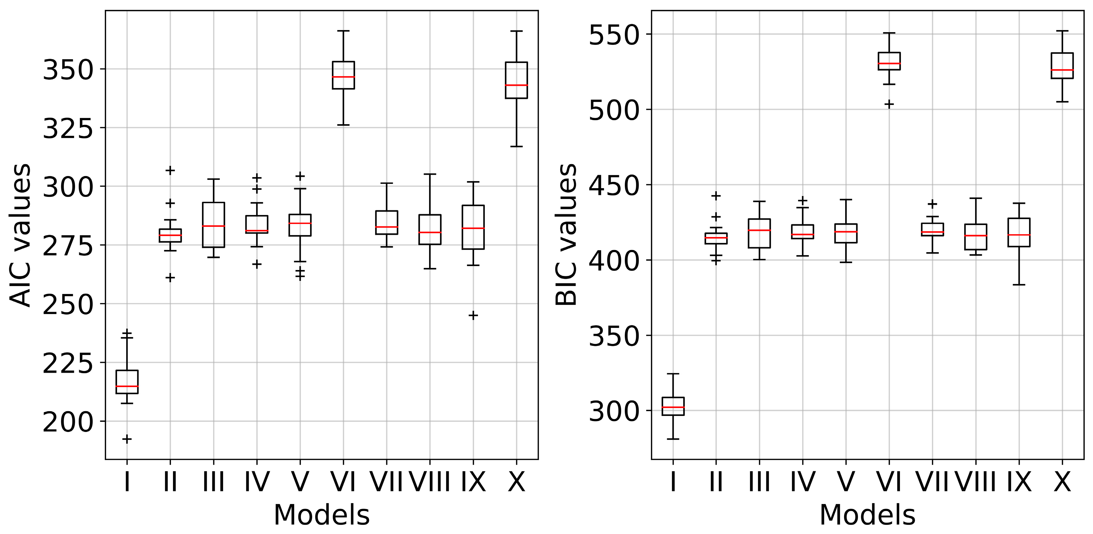
In addition, two performance measures were also carried out: Akaike Information Criteria (AIC) and Bayesian Information Criteria (BIC). These indices have the singularity of considering the number of trained parameters and they are based on the parsimony. AIC and BIC were initially reported by [84] and [85], respectively, and they have been frequently used for assessing hydrological models [86,87,88]. Both expressions are described in Equations (6) and (7):

$$AIC=N\ln \left(RMSE\right)+2p$$

(6)

$$BIC=N\ln \left(RMSE\right)+p \ln \left(N\right)$$

(7)

where p is the number of free parameters in each model (the total amount of weights and biases), being the best model performance the one with lowest AIC and BIC values. These indices deal with the trade-off between the prediction error (RMSE) and the complexity of the model, combining a term reflecting how well the forecasts fit the data with a term penalizing the model in proportion to its number of estimated parameters [89].

3. Results and Discussion

3.1. Pre-Processing Input Datasets

Validated daily records (precipitation, maximum and minimum temperature) obtained after the application of quality control procedures were used to create different monthly datasets. Monthly precipitation (P) values were used as an input in all the models assessed. Apart from max/min monthly temperature records (T_x and T_n, respectively), various temperature-based monthly time series were also created from daily values: mean daily temperature range (DTR_m), maximum daily temperature range (DTR_x), minimum daily temperature range (DTR_n) and monthly temperature range (MTR). Daily temperature range (DTR) is the difference between daily maximum temperature and daily minimum temperature, with DTR_m, DTR_x, DTR_n, being the mean, maximum and minimum DTR measured in a month, respectively. MTR is obtained as the difference between the maximum and minimum temperature measured in a monthly basis.

3.2. Performance of the Models

In general, regarding forecasted validation datasets and the common statistics, Model X was one of the best performers in most of the locations studied, although Model I showed the best results, on average, of BIC and AIC indices (Figure 5), followed by Models II, IX, VIII, V, IV, III, VII, X and VI. The minimum values obtained for both indices by using Models I, II, IX and X were registered in the driest location (Tabernas station), in Conil de la Frontera by using Model III and Model VII, in Mancha Real by using Model IV, in IFAPA-Las Torres station by using Model VI and in Huércal-Overa station by using Model V and Model VIII. As in the results reported by [87], both indices produced the same model selection, with the exception of Model VII that showed the best AIC and BIC performances in Sabiote and Conil de la Frontera stations, respectively. Overall, the results from BIC and AIC values indicated a worse performance of the approaches that use more variables (Model VI and Model X) than the rest, with Model I being the one with the lowest indices. Thus, the number of estimated parameters (weights and biases) in each of the models played a determining role in these indices.

In terms of the statistics R, RMSE, MAPE and NSE, the mean, maximum and minimum values obtained in the sixteen locations are summarized in

Table 4. Summary of correlation coefficient (R), root mean square error (RMSE), mean absolute percentage error (MAPE) and Nash–Sutcliffe model efficiency coefficient (NSE) values for all the models assessed.

Models	Datasets	R	RMSE (mm)	MAPE (%)	NSE
		Max/Mean/Min	Min/Mean/Max	Min/Mean/Max	Max/Mean/Min
I	Validation	0.78/0.70/0.62	9.39/21.69/37.74	9.82/33.94/52.52	0.62/0.51/0.40
	Calibration	0.83/0.74/0.65	11.75/20.67/29.60	9.86/16.07/22.57	0.81/0.72/0.63
II	Validation	0.80/0.69/0.55	10.73/31.55/44.03	25.34/39.93/62.02	0.67/0.50/0.32
	Calibration	0.98/0.92/0.79	11.89/16.18/29.21	1.86/7.84/22.99	0.96/0.85/0.63
III	Validation	0.84/0.71/0.56	13.75/24.17/39.53	11.39/31.57/49.86	0.73/0.54/0.33
	Calibration	0.95/0.92/0.87	11.33/17.59/26.97	4.92/8.63/15.91	0.91/0.84/0.75
IV	Validation	0.83/0.71/0.58	13.61/23.25/40.12	2.50/34.84/57.58	0.71/0.52/0.36
	Calibration	0.92/0.85/0.74	11.12/16.84/24.50	4.11/8.21/17.00	0.91/0.85/0.73
V	Validation	0.85/0.71/0.57	10.20/23.68/41.00	15.73/33.04/56.89	0.74/0.53/0.34
	Calibration	0.97/0.93/0.85	11.54/15.66/24.80	1.58/6.50/16.68	0.94/0.87/0.73
VI	Validation	0.89/0.73/0.59	12.64/22.48/38.51	9.80/31.19/48.17	0.82/0.55/0.37
	Calibration	0.97/0.95/0.91	7.79/13.96/18.28	0.12/5.05/11.89	0.95/0.90/0.82
VII	Validation	0.90/0.72/0.58	16.95/24.44/37.55	0.40/28.02/47.94	0.84/0.55/0.36
	Calibration	0.97/0.95/0.92	8.48/14.65/23.19	1.67/4.46/9.58	0.95/0.90/0.85
VIII	Validation	0.88/0.75/0.57	11.16/22.86/42.04	4.96/32.37/62.61	0.79/0.58/0.34
	Calibration	0.98/0.94/0.91	7.67/15.34/25.52	0.02/4.23/9.05	0.96/0.89/0.83
IX	Validation	0.90/0.74/0.57	6.79/22.84/38.17	3.45/28.05/41.50	0.84/0.58/0.35
	Calibration	0.97/0.94/0.88	8.02/15.03/21.22	1.67/5.09/11.15	0.94/0.89/0.77
X	Validation	0.90/0.82/0.64	8.49/21.49/38.39	4.57/23.61/40.04	0.83/0.69/0.44
	Calibration	0.98/0.94/0.90	9.61/14.61/20.88	2.45/5.71/11.40	0.96/0.89/0.81

for each model and dataset studied. Regarding validation forecasts, Model I obtained the best R (0.78) and NSE (0.62) values in Cártama station, and the lowest RMSE and MAPE values in Tabernas (9.39 mm) and El Campillo (9.82%) stations, respectively. On average, Model I had a generally better performance than other related models carried out in Greece [33] or in Jordan [83], but with R and NSE values lower than those reported by [68] in one station in India. However, Model II was the one that showed the worst results in almost all sites and for all the statistics studied, although with some exceptions. These results indicated that for the goal of this work, the information contained in the ‘two months before’ precipitation signal is not as relevant as the one contained in the ‘one month before’ signal. Model III had, on average, a slightly better performance, registering the lowest MAPE and RMSE values in Tabernas station (11.39% and 13.75 mm, respectively) and the best R (0.84) and NSE (0.73) values in El Carpio station. However, Model IV obtained good statistical indices in Cádiar, Mancha Real and Almería stations, while Model V gave the lowest RMSE (10.20 mm) in Huércal-Overa station. In general, the mean results obtained by using the variables DTR_m (Model III), DTR_x (Model IV) and DTR_n (Model V) were similar and better than those reported by [33] and [83], although in terms of MAPE, Model IV gave the best values in the most arid sites (Tabernas and Huércal-Overa stations). The next model assessed (VI) had a good performance in the two coastal locations: Conil de la Frontera station (highest R = 0.89 and NSE = 0.82 values) and Málaga station (best MAPE value = 9.80%), which may indicate that the joint use of DTR_x and DTR_n variables in areas near the sea could be recommended. Model VII gave the best MAPE values of all the models and sites in Cártama (0.40%) and IFAPA-Las Torres Tomejil (9.44%) stations and the best R (0.90), RMSE (16.95 mm) and NSE (0.84) values in Sabiote station, indicating that the new input variable MTR can be very useful in some locations. Finally, Model VIII (using T_x) obtained the lowest RMSE value in Huércal-Overa (11.16 mm), the best MAPE value in Sabiote (4.96%) and the highest R (0.88) and NSE (0.79) values in El Campillo station, where Model IX (using T_n) also obtained the lowest MAPE value (3.45%). In addition, this model (IX) had a very good behavior also in Sabiote (MAPE = 3.51%), Conil de la Frontera (R = 0.90 and NSE = 0.84), El Carpio (R = 0.85 and NSE = 0.75) and Tabernas (RMSE = 6.79 mm) stations. Regarding these last two models, no clear improvement was observed to recommend Model VII or Model IX based on the geo-climatic conditions. On average, the highest values of R (0.82) and NSE (0.69) were obtained by Model X (using T_x and T_n) for validation dataset and for all the sites, ranging from R = 0.90 and NSE = 0.83 (Conil de la Frontera station) to R = 0.64 and NSE = 0.44 (Húercal Overa station). In general, using Model II the lowest average values of R (0.69) and NSE (0.50) were given, and also the minimum values obtained for all the sites (R = 0.55 and NSE = 0.32 in Tabernas station). Regarding RMSE average values, they ranged from 21.49 (Model X) to 31.55 mm (Model II), while the highest value (44.03 mm) was registered in Jimena de la Frontera station by using also Model II, with this station being the one with the rainiest month (371.40 mm). Attending to MAPE average values, Model X was able to forecast with the lowest error (23.61%) followed by Model VII (28.02 %), ranging from 4.57% (Mancha Real station) to 40.04% (Écija station) and from 0.40% (Cártama station) to 47.94% (Santaella station), respectively. Instead, Model II gave the highest MAPE average value (39.93%) as well as the greatest percentage registered from all the stations (62.02%) in Cádiar (the highest location). As in other related works [3,32,34,68], a better general performance in calibration datasets can be observed.

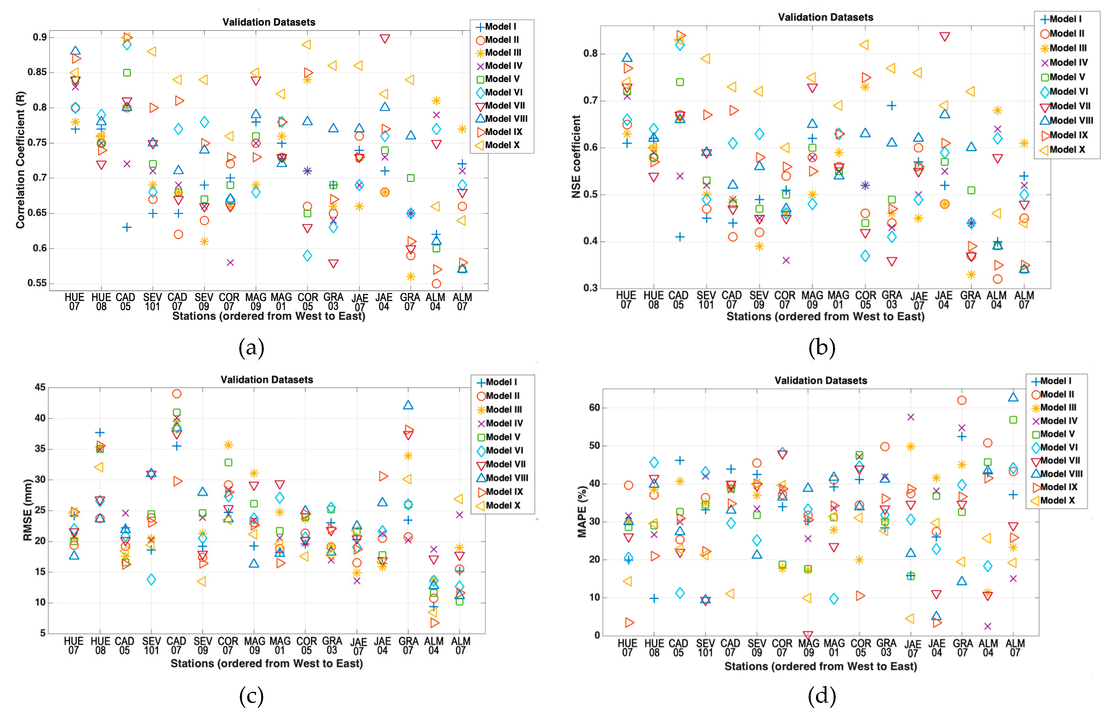
In order to evaluate the results obtained by using the ten models at each location, the statistical indices R, NSE, RMSE and MAPE are shown in Figure 6 (a, b, c and d, respectively) for validation datasets. In Figure 6a, it can be observed that in the most humid site (Puebla-Guzmán station = HUE07), located in the western region of Andalusia, the highest R (0.88) and NSE (0.79) values were obtained by Model VIII, followed by IX, X and VII. The other station situated in Huelva province (El Campillo station = HUE08) registered very homogeneous values of R and NSE by using all the models, with Model VI being the best one with values of 0.79 and 0.64, respectively. One of the best correlation coefficients and NSE values were obtained in Conil de la Frontera (CAD05) by using Model VI (R = 0.89 and NSE = 0.82), Model IX (R = 0.90 and NSE = 0.84) and Model X (R = 0.90 and NSE = 0.83). In this coastal location, Models IV and I gave the worst values. However, Model X was the best one for the following stations: IFAPA-Las Torres (SEV101), Jimena de la Frontera (CAD07), Écija (SEV09), Santaella (COR07), Cártama (MAG09), Málaga (MAG01), El Carpio (COR05), Loja (GRA03), Mancha Real (JAE07) and Cádiar (GRA07) stations (from West to East). Finally, for the driest locations (ALM04 = Tabernas and ALM07 = Huércal-Overa), situated in the eastern part of Andalusia, the model that derived the best R and NSE indices was the Model III, the one using DTR_m as input variable. Therefore, these results indicate that the use of DTR_m signal could be recommended for precipitation forecasting in arid stations. Considering Figure 6c, for the stations located in Huelva province (western part of Andalusia), the lowest RMSE values were obtained by Model VIII in HUE07 (17.60 mm) and HUE08 (23.62 mm), which could indicate the suitability of using this model in the less arid areas of Southern Spain. The location with the highest RMSE value was the rainiest site: Jimena de la Frontera (CAD07), while the lowest ones (6.79 and 10.20 mm) were obtained at the most arid stations by using Models IX (ALM04) and V (ALM07), respectively. Finally, MAPE values (Figure 6d) showed high variability between stations and also for the different models evaluated. The highest range between the best and the worst models was obtained in Mancha Real (JAE07), while the most homogeneous values occurred in Loja (GRA03). On average, the worst MAPE values were obtained in the highest location (Cádiar = GRA07), but no relationship was found between elevation and MAPE. For all the locations studied, several models were able to obtain MAPE values lower than 25%, including excellent performances such as those given by Model IX in Puebla Guzmán (HUE07), Model VII in Cártama (MAG09) or Model IV in Tabernas (ALM04), with the exception of Model X in Loja station (GRA03) obtaining 27.61%.

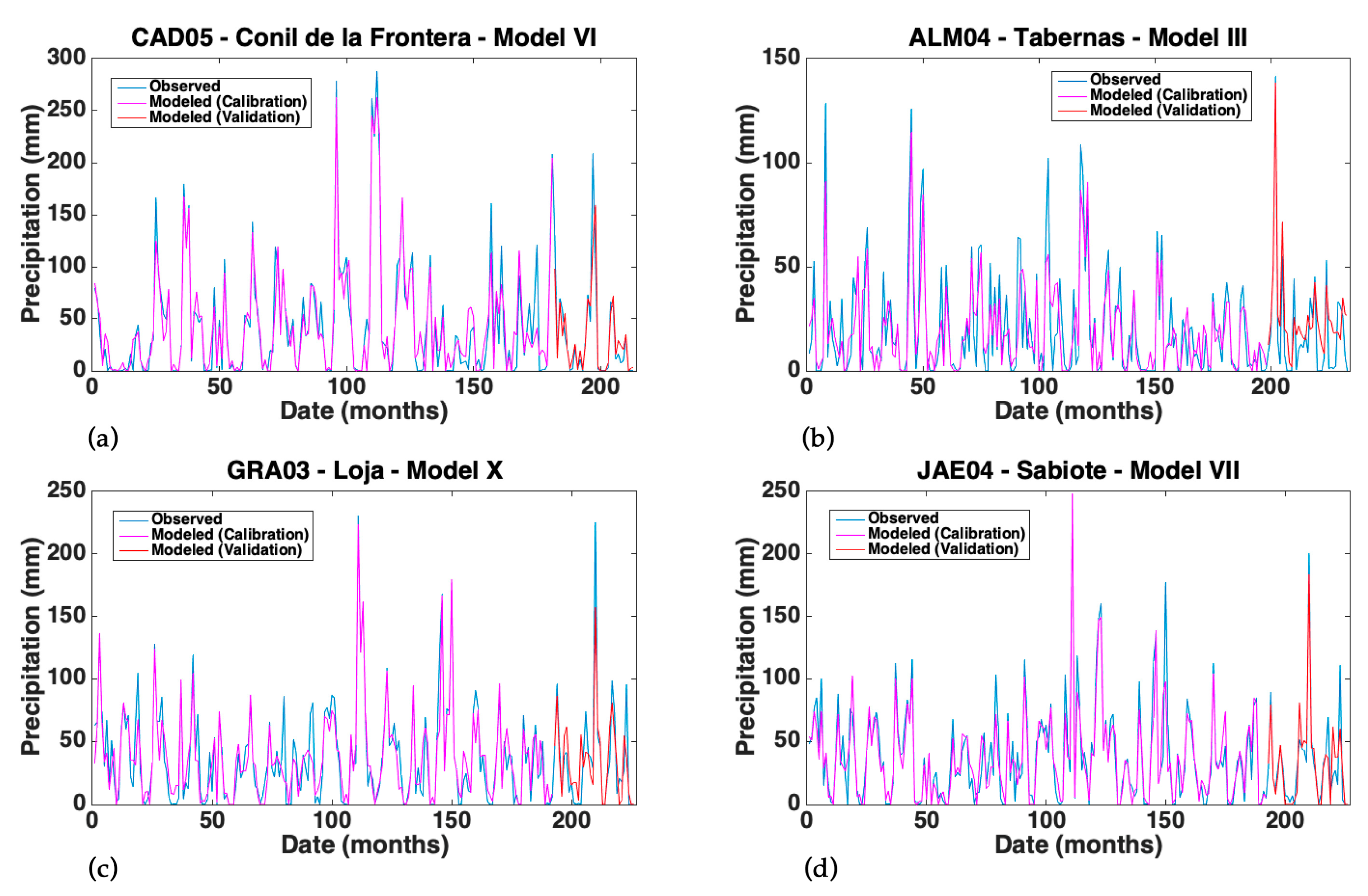
Finally, measured and forecasted values of monthly precipitation at four stations (Conil de la Frontera, Tabernas, Loja and Sabiote) during calibration and validation periods are represented in Figure 7. When attending to the validation datasets, a very good performance of Model VI can be observed in a coastal location such as Conil de la Frontera (CAD05), using MOY, precipitation, DTR_x and DTR_n as input variables and obtaining R = 0.89 and MAPE = 11.29%. In addition, this model also gave the lowest percentages of error at Málaga (MAG01) coastal station (MAPE = 9.80%). Thus, the input variables used in this model were more efficient at coastal locations than other variable combinations in terms of predictability performance. Slightly worse was the behavior of Model III (MOY, precipitation and DTR_m as input variables) in Tabernas (the driest station), with R=0.81, and MAPE = 11.39%, but being able to properly forecast the peak of 141.40 mm. Likewise, the validation period results obtained in Loja station (GRA03) by applying Model X indicated, in general, a satisfactory performance in terms of R (0.86), RMSE (17.81 mm) and NSE (0.72), although the peak of 225.40 mm was not predicted so accurately. Finally, the modelled datasets using Model VII in Sabiote station (JAE04) are represented. Regarding the validation period, the values of NSE, R and RMSE obtained with this model showed the best model performance in this site (0.84, 0.90 and 16.95 mm, respectively) and also giving an acceptable MAPE of 11.18%. Furthermore, this model that used MOY, precipitation and MTR as input variables, forecasted with lowest MAPE values in another two interior stations: Cártama (MAG09) and IFAPA-Las Torres Tomejil (SEV101), although its performance was not so good in other inland locations.

From these results, it has been verified that the introduction of easily estimated input variables such as DTR_x, DTR_n, DTR_m, MTR or MOY into WNN models is very useful for improving precipitation predictions one month ahead, especially when there is no availability of long-term datasets. In general, the results obtained by applying the proposed models in all stations in Southern Spain provided better RMSE values than the best of several WNN monthly precipitation models assessed by [68] at one station located in the east of India and also better than those reported by [3] at 24 locations in China, with both works needing the use of long-term historical series. Moreover, RMSE values were also lower in this work than the reported by [2] in ten stations in Guilin (China) using evolutionary models. In terms of efficiency, mean NSE values indicated a good degree of efficiency for all the models, being much higher than the values reported by [90] in Iran using ANN to predict monthly precipitation using 30-year series. RMSE values obtained with ANN models by [90] were worse than those given with the ten approaches assessed in this work. In addition, the correlation coefficients obtained in this work in all locations except at Huércal-Overa and Santaella sites were better than those reported by [33] in four stations in Greece for cumulative four-month precipitation predictions using ANN models. Regarding this statistic, the best result reported by [83] for the monthly precipitation in one of the three stations studied in Jordan was similar to the best values obtained in Santaella and Huércal-Overa stations but lower than those given in the rest of the locations. However, the correlation coefficient obtained by [90] with ANN and singular spectrum analysis model was better than the average performance of all the models, although models from V to X gave higher R values at least in one location of the sixteen sites evaluated.

4. Conclusions

Different configurations of hybrid model combining wavelet analysis and artificial neural network for time series forecasting of monthly precipitation have been developed and assessed at sixteen locations in Southern Spain (semiarid region). The main novelty of this work is the use of thermal variables, besides precipitation, never used before, such as the daily and monthly thermal range, as well as the month of year, the use of short-term time series and the application to datasets from sixteen sites having very different climatic and geographical conditions. Firstly, a set of sub-signals were obtained from original validated datasets carrying out a multilevel decomposition process by wavelet transformation. Then, these new time-series and months of year were used as input variables of the ten models evaluated, with original monthly precipitation being the output variable. The models were calibrated using the first 85% of datasets and the rest of the data were used for model validation (at least two and a half years at all locations). The results indicated that nonlinear dynamics of the different thermal variables used and also precipitation were properly characterized by wavelet decomposition in order to satisfactorily forecast precipitation one month ahead, although the performance of the models was not the same for the different locations evaluated. For each location, it was found that there was at least one or more models with acceptable statistical performance (R > 0.76; NSE > 0.60; RMSE < 29.82 mm and MAPE < 27.62%).

In general, the model that used precipitation, maximum and minimum temperature (X) had the best statistical performance in most of the locations studied. However, the model using precipitation and the mean diurnal temperature range (III) gave the best results at the most arid sites. Regarding coastal locations, the lowest mean absolute percentage of errors were obtained by the model using precipitation, maximum and minimum diurnal temperature range (VI). By contrast, the model using only precipitation signal (I) obtained the best BIC at all locations and the lowest AIC values at twelve sites due to the reduced number of input variables but did not get the best results in any other statistical indices except in El Campillo station, the second rainiest site of this study. Although no relationship between model performance and site elevation was found, the worst mean absolute percentage error was obtained in the highest site studied (Cádiar station). Finally, the model using precipitation and monthly temperature range (VII) gave satisfactory results in terms of predictability error in three interior locations. Therefore, overall analysis of the general results obtained in this work indicates the suitability of the type of input variables used in WNN models that accurately describe precipitation processes according to geo-climatic characteristics.

Since most of the thermo-pluviometric sensors installed on automatic weather stations networks worldwide do not have long-term time series and considering that precipitation is a meteorological variable with high spatial variability, these types of models are of great interest to the monthly precipitation forecast in locations where only short length records are available. Further works using different artificial intelligence approaches such as support vector machine or extreme learning machine may be carried out to compare the performance of these kind of models once they are joined to wavelet analysis.

References

- Linnerud, K.; Mideksa, T.K.; Eskeland, G.S. The impact of climate change on nuclear power supply. Energy J. 2011, 32, 149–168. [Google Scholar] [CrossRef]
- Jiang, L.; Wu, J. Hybrid PSO and GA for neural network evolutionary in monthly rainfall forecasting. In Asian Conference on Intelligent Information and Database Systems; Selamat, A., Nguyen, N.T., Haron, H., Eds.; Springer: Berlin/Heidelberg, Germany, 2013; Volume 7802, pp. 79–88. [Google Scholar]
- Liu, Q.; Zou, Y.; Liu, X.; Linge, N. A survey on rainfall forecasting using artificial neural network. Int. J. Embed. Syst. 2019, 11, 240–249. [Google Scholar] [CrossRef] [Green Version]
- Jabbari, A.; Bae, D.-H. Application of artificial neural networks for accuracy enhancements of real-time flood forecasting in the Imjin Basin. Water 2018, 10, 1626. [Google Scholar] [CrossRef] [Green Version]
- Alotaibi, K.; Ghumman, A.R.; Haider, H.; Ghazaw, Y.M.; Shafiquzzaman, M. Future predictions of rainfall and temperature using GCM and ANN for arid regions: A case study for the Qassim Region, Saudi Arabia. Water 2018, 10, 1260. [Google Scholar] [CrossRef] [Green Version]
- Moghim, S.; Bras, R.L. Bias correction of climate modeled temperature and precipitation using artificial neural networks. J. Hydrometeorol. 2017, 18, 1867–1884. [Google Scholar] [CrossRef]
- Yang, Z.; Hsu, K.; Sorooshian, S.; Xu, X.; Braithwaite, D.; Verbist, K.M. Bias adjustment of satellite-based precipitation estimation using Gauge Observations—A case study in Chile. J. Geophys. Res. Atmos. 2016, 121, 3790–3806. [Google Scholar] [CrossRef] [Green Version]
- Crochemore, L.; Ramos, M.H.; Pappenberger, F. Bias correcting precipitation forecasts to improve the skill of seasonal streamflow forecasts. Hydrol. Earth Syst. Sci. 2016, 20, 3601–3618. [Google Scholar] [CrossRef] [Green Version]
- Ramírez, M.C.V.; de Campos Velho, H.F.; Ferreira, N.J. Artificial neural network technique for rainfall forecasting applied to the São Paulo region. J. Hydrol. 2005, 301, 146–162. [Google Scholar] [CrossRef]
- Darji, M.; Dabhi, V.; Prajapati, H. Rainfall forecasting using neural network: A survey. In Proceedings of the 2015 International Conference on Advances in Computer Engineering and Applications (IEEE), Ghaziabad, India, 19–20 March 2015; pp. 706–707. [Google Scholar]
- Nanda, S.K.; Tripathy, D.P.; Nayak, S.K.; Mohapatra, S. Prediction of rainfall in India using Artificial Neural Network (ANN) models. Int. J. Intell. Syst. Appl. 2013, 5, 1. [Google Scholar] [CrossRef]
- Geetha, G.; Selvaraj, R.S. Prediction of monthly rainfall in Chennai using back propagation neural network model. Int. J. Eng. Sci. Technol. 2011, 3, 211–213. [Google Scholar]
- McCulloch, W.S.; Pitts, W. A logical calculus of the ideas immanent in nervous activity. Bull. Math. Biophys. 1943, 5, 115–133. [Google Scholar] [CrossRef]
- Rumelhart, D.E.; Hinton, G.E.; Williams, R.J. Learning representations by back-propagating errors. Nature 1986, 323, 533–536. [Google Scholar] [CrossRef]
- Maier, H.R.; Dandy, G.C. The use of artificial neural networks for the prediction of water quality parameters. Water Resour. Res. 1996, 32, 1013–1022. [Google Scholar] [CrossRef]
- French, M.; Krajewski, W.; Cuykendall, R. Rainfall forecasting in space and time using a neural network. J. Hydrol. 1992, 137, 1–31. [Google Scholar] [CrossRef]
- Kumar, A.S.; Sudheer, K.; Jain, S.; Agarwal, P. Rainfall-runoff modelling using artificial neural networks: Comparison of network types. Hydrol. Process. 2005, 19, 1277–1291. [Google Scholar] [CrossRef]
- Fernando, D.A.K.; Jayawardena, A.W. Runoff forecasting using RBF networks with OLS algorithm. J. Hydrol. Eng. 1998, 3, 203–209. [Google Scholar] [CrossRef]
- Dawson, C.; Wilby, R. An artificial neural network approach to rainfall-runoff modeling. Hydrol. Sci. J. 1998, 43, 47–66. [Google Scholar] [CrossRef]
- Jeong, D.I.; Kim, Y.-O. Rainfall-runoff models using artificial neural networks for ensemble streamflow prediction. Hydrol. Process. 2005, 19, 3819–3835. [Google Scholar] [CrossRef]
- Riad, S.; Mania, J.; Bouchaou, L.; Najjar, Y. Predicting catchment flow in a semi-arid region via an artificial neural network technique. Hydrol. Process. 2004, 18, 2387–2393. [Google Scholar] [CrossRef]
- Birikundavyi, S.; Labib, R.; Trung, H.T.; Rousselle, J. Performance of neural networks in daily streamflow forecasting. J. Hydrol. Eng. 2002, 7, 392–398. [Google Scholar] [CrossRef]
- Kim, R.; Loucks, P.; Stedinger, J. Artificial neural network models of watershed nutrient loading. Water Res. Manag. 2012, 26, 2781–2797. [Google Scholar] [CrossRef]
- Zaheer, I.; Bai, C.-G. Application of artificial neural network for water quality management. Lowl. Technol. Int. 2003, 5, 10–15. [Google Scholar]
- Nourani, V.; Mousavi, S. Spatiotemporal groundwater level modeling using hybrid artificial intelligence-meshless method. J. Hydrol. 2016, 536, 10–25. [Google Scholar] [CrossRef]
- Talei, A.; Chua, L.H.C.; Wong, T.S. Evaluation of rainfall and discharge inputs used by Adaptive Network-based Fuzzy Inference Systems (ANFIS) in rainfall–runoff modeling. J. Hydrol. 2010, 391, 248–262. [Google Scholar] [CrossRef]
- López-Lineros, M.; Estévez, J.; Giráldez, J.V.; Madueño, A. A new quality control procedure based on non-linear autoregressive neural network for validating raw river stage data. J. Hidrol. 2014, 510, 103–109. [Google Scholar] [CrossRef]
- Sciuto, G.; Bonaccorso, B.; Cancelliere, A.; Rossi, G. Quality control of daily rainfall data with neural networks. J. Hydrol. 2009, 364, 13–22. [Google Scholar] [CrossRef]
- Govindaraju, R. Artificial Neural Networks in hydrology. II: Hydrologic applications. J. Hydrol. Eng. 2000, 5, 124–137. [Google Scholar]
- Govindaraju, R. Artificial neural networks in hydrology. I: Preliminary concepts. J. Hydrol. Eng. 2000, 5, 115–123. [Google Scholar]
- Oyebode, O.; Stretch, D. Neural network modeling of hydrological systems: A review of implementation techniques. Nat. Resour. Model. 2019, 32, e12189. [Google Scholar] [CrossRef] [Green Version]
- Hung, N.Q.; Babel, M.S.; Weesakul, S.; Tripathi, N. An artificial neural network model for rainfall forecasting in Bangkok, Thailand. Hydrol. Earth Syst. Sci. 2009, 13, 1413–1425. [Google Scholar] [CrossRef] [Green Version]
- Moustris, K.P.; Larissi, I.K.; Nastos, P.T.; Paliatsos, A.G. Precipitation forecast using artificial neural networks in specific regions of Greece. Water Res. Manag. 2011, 25, 1979–1993. [Google Scholar] [CrossRef]
- Lee, J.; Kim, C.G.; Lee, J.E.; Kim, N.W.; Kim, H. Application of artificial neural networks to rainfall forecasting in the Geum River basin, Korea. Water 2018, 10, 1448. [Google Scholar] [CrossRef] [Green Version]
- Abbot, J.; Marohasy, J. Forecasting of medium-term rainfall using Artificial Neural Networks: Case studies from Eastern Australia. In Engineering and Mathematical Topics in Rainfall; IntechOpen: London, UK, 2018; Volume 33. [Google Scholar]
- Yang, Y.; Luo, Y. Using the back propagation neural network approach to bias correct TMPA data in the arid region of Northwest China. J. Hydrometeorol. 2014, 15, 459–473. [Google Scholar] [CrossRef] [Green Version]
- Wu, X.; Hongxing, C.; Flitman, A.; Fengying, W.; Guolin, F. Forecasting monsoon precipitation using artificial neural networks. Adv. Atmos. Sci. 2001, 18, 950–958. [Google Scholar] [CrossRef]
- Tyagi, N.; Kumar, A. Comparative analysis of backpropagation and RBF neural network on monthly rainfall prediction. In Proceedings of the 2016 International Conference on Inventive Computation Technologies (ICICT), Coimbatore, India, 26–27 August 2016; pp. 1–6. [Google Scholar]
- Manek, A.; Singh, P. Comparative study of neural network architectures for rainfall prediction. In Proceedings of the 2016 IEEE Technological Innovations in ICT for Agriculture and Rural Development (TIAR), Chennai, India, 15–16 July 2016; pp. 171–174. [Google Scholar]
- Goyal, M. Monthly rainfall prediction using wavelet regression and neural network: An analysis of 1901–2002 data, Assam, India. Theor. Appl. Climatol. 2014, 118, 25–34. [Google Scholar] [CrossRef]
- Acharya, N.; Shrivastava, N.; Panigrahi, B.K.; Mohanty, U.C. Development of an artificial neural network based multi-model ensemble to estimate the northeast monsoon rainfall over south peninsular India: An application of extreme learning machine. Clim. Dyn. 2014, 43, 1303–1310. [Google Scholar] [CrossRef]
- García-Marín, A.P.; Estévez, J.; Morbidelli, R.; Saltalippi, C.; Ayuso, J.; Flammini, A. Assessing inhomogeneities in extreme annual rainfall data series by multifractal approach. Water 2020, 12, 1030. [Google Scholar] [CrossRef] [Green Version]
- Bohlinger, P.; Sorteberg, A.; Liu, C.; Rasmussen, R.; Sodemann, H.; Ogawa, F. Multiscale characteristics of an extreme precipitation event over Nepal. Q. J. R. Meteorol. Soc. 2019, 145, 179–196. [Google Scholar] [CrossRef] [Green Version]
- Medina-Cobo, M.; García-Marín, A.P.; Estévez, J.; Jiménez-Hornero, F.; Ayuso, J. Obtaining homogeneous regions by determining the generalized fractal dimensions of validated daily rainfall data sets. Water Res. Manag. 2017, 31, 2333–2348. [Google Scholar] [CrossRef]
- Medina-Cobo, M.T.; García-Marín, A.P.; Estévez, J.; Ayuso-Muñoz, J.L. The identification of an appropriate Minimum Inter-event Time (MIT) based on multifractal characterization of rainfall data series. Hydrol. Process. 2016, 30, 3507–3517. [Google Scholar] [CrossRef]
- García-Marín, A.P.; Estévez, J.; Medina-Cobo, M.T.; Ayuso, J. Delimiting homogeneous regions using the multifractal properties of validated rainfall data series. J. Hydrol. 2015, 529, 106–119. [Google Scholar] [CrossRef]
- Samuel, J.M.; Sivapalan, M. A comparative modeling analysis of multiscale temporal variability of rainfall in Australia. Water Resour. Res. 2008, 44, W07401. [Google Scholar] [CrossRef]
- Estévez, J.; García-Marín, A.P.; Benitez, J.B.; Castillo, M.C.C.; Telesca, L. Introduction to the special issue on “hydro-meteorological time series analysis and their relation to climate change”. Acta Geophys. 2018, 66, 317–318. [Google Scholar] [CrossRef]
- Grossmann, A.; Morlet, J. Decomposition of Hardy functions into square integrable wavelets of constant shape. SIAM J. Math. Anal. 1984, 15, 723–736. [Google Scholar] [CrossRef]
- Sang, Y.-F. A review on the applications of wavelet transform in hydrology time series analysis. Atmos. Res. 2013, 122, 8–15. [Google Scholar] [CrossRef]
- Maheswaran, R.; Khosa, R. Comparative study of different wavelets for hydrologic forecasting. Comput. Geosci. 2012, 46, 284–295. [Google Scholar] [CrossRef]
- Adamowski, J.; Chan, H.F. A wavelet neural network conjunction model for groundwater level forecasting. J. Hydrol. 2011, 407, 28–40. [Google Scholar] [CrossRef]
- Baddoo, T.; Guan, Y.; Zhang, D.; Andam-Akorful, S. Rainfall variability in the Huangfuchuang Watershed and its relationship with ENSO. Water 2015, 7, 3243–3262. [Google Scholar] [CrossRef] [Green Version]
- Wang, Y.; Yuan, Y.; Pan, Y.; Fan, Z. Modeling daily and monthly water quality indicators in a canal using a hybrid wavelet-based support vector regression structure. Water 2020, 12, 1476. [Google Scholar] [CrossRef]
- Daubechies, I. Ten Lectures on Wavelets; SIAM: Philadelphia, PA, USA, 1992. [Google Scholar]
- Guimarães-Santos, C.A.; Silva, G.B.L.D. Daily streamflow forecasting using a wavelet transform and artificial neural network hybrid models. Hydrol. Sci. J. 2014, 59, 312–324. [Google Scholar] [CrossRef]
- Nalley, D.; Adamowski, J.; Khalil, B. Using discrete wavelet transforms to analyze trends in streamflow and precipitation in Quebec and Ontario (1954–2008). J. Hydrol. 2012, 475, 204–228. [Google Scholar] [CrossRef]
- Benaouda, D.; Murtagh, F.; Starck, J.L.; Renaud, O. Wavelet-based nonlinear multiscale decomposition model for electricity load forecasting. Neurocomputing 2006, 70, 139–154. [Google Scholar] [CrossRef]
- WMO. Guide to Instruments and Methods of Observations; WMO: Geneva, Switzerland, 2018; Volume 8. [Google Scholar]
- Paola, F.; Giugni, M. Coupled spatial distribution of rainfall and temperature in USA. Procedia Environ. Sci. 2013, 19, 178–187. [Google Scholar] [CrossRef] [Green Version]
- Estévez, J.; Padilla, F.L.; Gavilán, P. Evaluation and regional calibration of solar radiation prediction models in southern Spain. J. Irrig. Drain. Eng. 2012, 138, 868–879. [Google Scholar] [CrossRef]
- Eccel, E. Estimating air humidity from temperature and precipitation measures for modelling applications. Meteorol. Appl. 2012, 19, 118–128. [Google Scholar] [CrossRef]
- Intergovernmental Panel on Climate Change. IPCC Fifth Assessment Report (AR5) Observed Climate Change Impacts Database; Version 2.01; NASA Socioeconomic Data and Applications Center (SEDAC): Palisades, NY, USA, 2017. [Google Scholar] [CrossRef]
- Chen, Z.; Yu, G.; Ge, J.; Sun, X.; Hirano, T.; Saigusa, N.; Wang, Q.; Zhu, X.; Zhang, Y.; Zhang, J.; et al. Temperature and precipitation control of the spatial variation of terrestrial ecosystem carbon exchange in the Asian region. Agric. For. Meteorol. 2013, 182, 266–276. [Google Scholar] [CrossRef]
- Lewis, E.; Fowler, H.; Alexander, L.; Dunn, R.; McClean, F.; Barbero, R.; Guerreiro, S.; Xiao-Feng, L.; Blenkinsop, S. GSDR: A global sub-daily rainfall dataset. J. Clim. 2019, 32, 4715–4729. [Google Scholar] [CrossRef]
- Strigaro, D.; Cannata, M.; Antonovic, M. Boosting a weather monitoring system in low income economies using open and non-conventional systems: Data quality analysis. Sensors 2019, 19, 1185. [Google Scholar] [CrossRef] [Green Version]
- Wei, S.; Yang, H.; Song, J.; Abbaspour, K.; Xu, Z. A wavelet-neural network hybrid modelling approach for estimating and predicting river monthly flows. Hydrol. Sci. J. 2013, 58, 374–389. [Google Scholar] [CrossRef]
- Ramana, R.V.; Krishna, B.; Kumar, S.R.; Pandey, N.G. Monthly rainfall prediction using wavelet neural network analysis. Water Res. Manag. 2013, 27, 3697–3711. [Google Scholar] [CrossRef] [Green Version]
- Wu, C.; Chau, K.; Li, Y. Methods to improve neural network performance in daily flows prediction. J. Hydrol. 2009, 372, 80–93. [Google Scholar] [CrossRef] [Green Version]
- Nourani, V.; Alami, M.T.; Aminfar, M.H. A combined neural-wavelet model for prediction of Ligvanchai watershed precipitation. Eng. Appl. Artif. Intel. 2009, 22, 466–472. [Google Scholar] [CrossRef]
- Gómez-Zotano, J.; Alcántara-Manzanares, J.; Olmedo-Cobo, J.A.; Martínez-Ibarra, E. La sistematización del clima mediterráneo: Identificación, clasificación y caracterización climática de Andalucía (España). Rev. Geogr. Norte Gd. 2015, 61, 161–180. [Google Scholar] [CrossRef] [Green Version]
- Estévez, J.; Gavilán, P.; Giráldez, J.V. Guidelines on validation procedures for meteorological data from automatic weather stations. J. Hydrol. 2011, 402, 144–154. [Google Scholar] [CrossRef] [Green Version]
- Estévez, J.; Gavilán, P.; García-Marín, A.P.; Zardi, D. Detection of spurious precipitation signals from automatic weather stations in irrigated areas. Int. J. Climatol. 2015, 35, 1556–1568. [Google Scholar] [CrossRef]
- Estévez, J.; Gavilán, P.; García-Marín, A.P. Spatial regression test for ensuring temperature data quality. Theor. Appl. Climatol. 2018, 131, 309–318. [Google Scholar] [CrossRef]
- Nourani, V.; Elkiran, G.; Abdullahi, J. Multi-station artificial intelligence based ensemble modeling of reference evapotranspiration using pan evaporation measurements. J. Hydrol. 2019, 577, 123958. [Google Scholar] [CrossRef]
- Islam, A.T.; Shen, S.; Yang, S.; Hu, Z.; Chu, R. Assessing recent impacts of climate change on design water requirement of Boro rice season in Bangladesh. Theor. Appl. Climatol. 2019, 138, 97–113. [Google Scholar] [CrossRef]
- Yi, Z.; Zhao, H.; Jiang, Y. Continuous daily evapotranspiration estimation at the field-scale over heterogeneous agricultural areas by fusing aster and modis data. Remote Sens. 2018, 10, 1694. [Google Scholar] [CrossRef] [Green Version]
- Estévez, J.; García-Marín, A.P.; Morábito, J.A.; Cavagnaro, M. Quality assurance procedures for validating meteorological input variables of reference evapotranspiration in mendoza province (Argentina). Agric. Water Manag. 2016, 172, 96–109. [Google Scholar] [CrossRef]
- Wang, W.; Van Gelder, P.H.; Vrijling, J.; Ma, J. Forecasting daily streamflow using hybrid ANN models. J. Hydrol. 2006, 324, 383–399. [Google Scholar] [CrossRef]
- Pal, L.; Ojha, C.S.P.; Chandniha, S.K.; Kumar, A. Regional scale analysis of trends in rainfall using nonparametric methods and wavelet transforms over a semi-arid region in India. Int. J. Climatol. 2019, 39, 2737–2764. [Google Scholar] [CrossRef]
- Shoaib, M.; Shamseldin, A.Y.; Melville, B.W. Comparative study of different wavelet based neural network models for rainfall–runoff modeling. J. Hydrol. 2014, 515, 47–58. [Google Scholar] [CrossRef]
- Du, K.; Zhao, Y.; Lei, J. The incorrect usage of singular spectral analysis and discrete wavelet transform in hybrid models to predict hydrological time series. J. Hydrol. 2017, 552, 44–51. [Google Scholar] [CrossRef]
- Aksoy, H.; Dahamsheh, A. Artificial neural network models for forecasting monthly precipitation in Jordan. Stoch. Environ. Res. Risk Assess. 2009, 23, 917–931. [Google Scholar] [CrossRef]
- Akaike, H. A new look at the statistical model identification. IEEE Trans. Autom. Control 1974, 19, 716–723. [Google Scholar] [CrossRef]
- Rissanen, J. Modeling by shortest data description. Automatica 1978, 14, 465–471. [Google Scholar] [CrossRef]
- Nourani, V.; Komasi, M. A geomorphology-based ANFIS model for multi-station modeling of rainfall-runoff process. J. Hydrol. 2013, 490, 41–55. [Google Scholar] [CrossRef]
- Laio, F.; Di Baldassarre, G.; Montanari, A. Model selection techniques for the frequency analysis of hydrological extremes. Water Resour. Res. 2009, 45, W07416. [Google Scholar] [CrossRef]
- Dawson, C.; Wilby, R. Hydrological modelling using artificial neural networks. Prog. Phys. Geogr. 2001, 25, 80–108. [Google Scholar] [CrossRef]
- Kriegeskorte, N. Crossvalidation, in Brain Mapping; Toga, A.W., Ed.; Academic Press: Waltham, UK, 2015; pp. 635–639. [Google Scholar]
- Kalteh, A.M. Enhanced monthly precipitation forecasting using artificial neural network and singular spectrum analysis conjunction models. INAE Lett. 2017, 2, 73–81. [Google Scholar] [CrossRef] [Green Version]
Figure 1.
Wavelet multiresolution analysis of original time-series.
Figure 2.
Geographical distribution of the automated weather stations used in this work (Andalusia region—Southern Spain).
Figure 3.
Multilayer Perceptron Neural Network architecture used in this work.
Figure 4.
Original values and decomposed sub-series of monthly precipitation by wavelet transformation at Málaga station (MAG01) (2001–2019).
Figure 5.
Box-plot of the Akaike Information Criteria (AIC) and Bayesian Information Criteria (BIC) values obtained by using the ten models (validation datasets) for all the sites studied. On each box: the red central mark=median; bottom and top edges of the box = 25th and 75th percentiles, respectively; whiskers extend to the most extreme values are not considered outliers (‘+’ symbol).
Figure 6.
Results of the statistical performance obtained at each of the 16 locations studied: (a) R; (b) NSE; (c) RMSE; (d) MAPE.
Figure 7.
Plot of measured and forecasted monthly precipitation at four stations: Conil de la Frontera (a), Tabernas (b), Loja (c) and Sabiote (d) using Models VI, III, X and VIII, respectively.