Effect of Logarithmically Transformed IMERG Precipitation Observations in WRF 4D-Var Data Assimilation System


1
School of Civil and Environmental Engineering, Georgia Institute of Technology, Atlanta, GA 30332, USA
2
NOAA/OAR/Global Systems Laboratory, Boulder, CO 80305, USA
3
Cooperative Institute for Research in the Atmosphere, Colorado State University, Fort Collins, CO 80523, USA
*
Author to whom correspondence should be addressed.
Water 2020, 12(7), 1918; https://doi.org/10.3390/w12071918
Submission received: 21 May 2020
/
Revised: 17 June 2020
/
Accepted: 28 June 2020
/
Published: 5 July 2020
(This article belongs to the Special Issue Hydrometeorological Forecasting Using the Weather Research and Forecasting Model)
Abstract
:Precipitation estimates from numerical weather prediction (NWP) models are uncertain. The uncertainties can be reduced by integrating precipitation observations into NWP models. This study assimilates Version 04 Integrated Multi-satellite Retrievals for the Global Precipitation Measurement (GPM) (IMERG) Final Run into the Weather Research and Forecasting (WRF) model data assimilation (WRFDA) system using a four-dimensional variational (4D-Var) method. Three synoptic-scale convective precipitation events over the central United States during 2015–2017 are used as case studies. To investigate the effect of logarithmically transformed IMERG precipitation in the WRFDA system, this study reports on several experiments with six-hour and hourly assimilation windows, regular (nontransformed) and logarithmically transformed observations, and a constant observation error in regular and logarithmic spaces. Results show that hourly assimilation windows improve precipitation simulations significantly compared to six-hour windows. Logarithmically transformed precipitation does not improve precipitation estimations relative to nontransformed precipitation. However, better predictions of heavy precipitation can be achieved with a constant error in the logarithmic space (corresponding to a linearly increasing error in the regular space), which modifies the threshold of rejecting observations, and thus utilizes more observations. This study provides a cost function with logarithmically transformed observations for the 4D-Var method in the WRFDA system for future investigations.
1. Introduction
Precipitation is an important component of the water cycle. It influences hydrologic variables, such as groundwater flow and runoff, which are vital to our daily life. Accurate estimates of precipitation are of great value for society. However, model simulations of precipitation usually have uncertainties [1,2]. One reason is the uncertainty of the initial condition of the model [3]. Very small differences in the initial condition can cause diverging simulations of the climate system. One possible solution to the uncertainty of the initial condition is to integrate precipitation observations into the model [4,5].
The assimilation of precipitation has been widely studied in recent decades. Among the various approaches for assimilating precipitation, the four-dimensional variational (4D-Var) method is one of the most commonly used [6,7,8,9,10,11,12,13]. In the cost function of the 4D-Var method (see Section 2.1.1), observation errors are assumed to be Gaussian distributed. However, the errors in short-interval precipitation observations do not have Gaussian properties [8,14]. To solve this problem, Koizumi et al. [8] assumed an exponential distribution for precipitation and derived a new cost function for the 4D-Var method. Lopez [9] used the original cost function but applied a logarithmic transformation on precipitation intensity before assimilation at the European Centre for Medium-Range Weather Forecasts (ECMWF) Global Integrated Forecasting System. Lien et al. [15] further proposed logarithmic and Gaussian transformations on precipitation intensity in the National Center for Environmental Prediction (NCEP) Global Forecast System (GFS); the same authors [16] suggested that either a logarithmic or a Gaussian transformation would be necessary to improve precipitation analyses and forecasts. In the Weather Research and Forecasting (WRF) model data assimilation (WRFDA) system, however, assimilation of transformed precipitation has not been tested.
There are two types of precipitation observations: ground- and satellite-based products. Ground-based products, such as gauges and ground-radar estimates, have high accuracy, but they are limited in space. Although satellite-based products are less accurate due to retrieval algorithms [17,18], they have great value in global applications because of their global coverage [19,20]. Moreover, with the development and improvement of techniques for satellite retrievals, the quality of satellite precipitation products is improving [19,21,22,23,24]. To understand the benefit of assimilating satellite precipitation products into model systems, this study will assimilate precipitation data from the Integrated Multisatellite Retrievals for the Global Precipitation Measurement (GPM) (IMERG) into the WRFDA system using the 4D-Var method. The objective of this study is to test the impact of logarithmically transformed IMERG precipitation in the WRF 4D-Var system.
2. Materials and Methods
2.1. The 4D-Var Method
2.1.1. Cost Function with Nontransformed Observations
The 4D-Var data assimilation method is embedded in the WRFDA system. The aim of 4D-Var assimilation is to find the optimal initial state , which is also called the analysis , by iteratively minimizing the following cost function [25]:
where the state consists of temperature, pressure, zonal and meridional winds, and humidity; is the background state at initial time, and is its error covariance matrix; is the model operator that predicts state variables at time , and is the observation operator that transforms the state variables into the form of observations; is the observation at time , and is its error covariance. In this study, because we assimilate precipitation only at the end of assimilation windows, there is only one time-interval for observations (i.e., ).
In the WRFDA system, the cost function is reformulated using an incremental approach [26]:
where is the increment relative to the first guess , and is the difference between the background and the first guess. The background is the initial condition of model simulations, and the first guess varies with outer iterative loops of minimization. For the first outer loop, the first guess is equal to the background. From the second outer loop on, the first guess is equal to the analysis of the previous outer loop. Following Ban et al. [12], we apply two outer loops in this study. In Equation (2), is the innovation vector, and and are the tangent linear versions of and , respectively. Observations are rejected if they depart too much from model predictions:
where is the standard deviation of observation error, , and we follow previous studies and set [10].
2.1.2. Cost Function with Logarithmically Transformed Observations
Because a transformation of precipitation intensity is necessary to avoid suboptimal 4D-Var analyses [16,27], this study will test the WRF 4D-Var system with a logarithmic transformation on precipitation as Lopez [9] did in the ECMWF Global Integrated Forecasting system. The incremental form of the cost function after transformation changes to
where is the tangent linear version of the logarithmic transformation operator , which transforms both the intensity and the error structure of observations:
The transformation also changes the constraint for observations being rejected:
where is the standard deviation of the transformed observations : . The derivations of the transformed incremental cost function and error structure are provided in Equations (A1)–(A6) in Appendix A.
2.2. Precipitation Observations
The precipitation observations () used in this study are hourly and six-hour accumulations from Version 04 IMERG Final Run. The IMERG product combines precipitation estimates from all passive microwave sensors from the GPM constellation, infrared observations from geosynchronous satellites, and is adjusted to monthly gauge measurements [28]. The IMERG product covers the globe from 60° S to 60° N with a spatial resolution of 0.1° and a temporal resolution of 30 min. The datasets are available on the Precipitation Measurement Missions (PMM) website (https://pmm.nasa.gov/data-access/downloads/gpm), and detailed information is given in Huffman et al. [28,29]. To assimilate the IMERG precipitation observations into the 4D-Var WRFDA system, the observation error covariance is assumed to be block diagonal, which means that there is no spatial correlation among observations [9]. We assign a constant error (0.3 mm/h for hourly precipitation and 2 mm/6 hr for six-hour accumulated precipitation) in the regular space and in the logarithmic space. The error 0.3 mm/h in the logarithmic space corresponds to 0.3 mm/h in the regular space according to Equation 6.
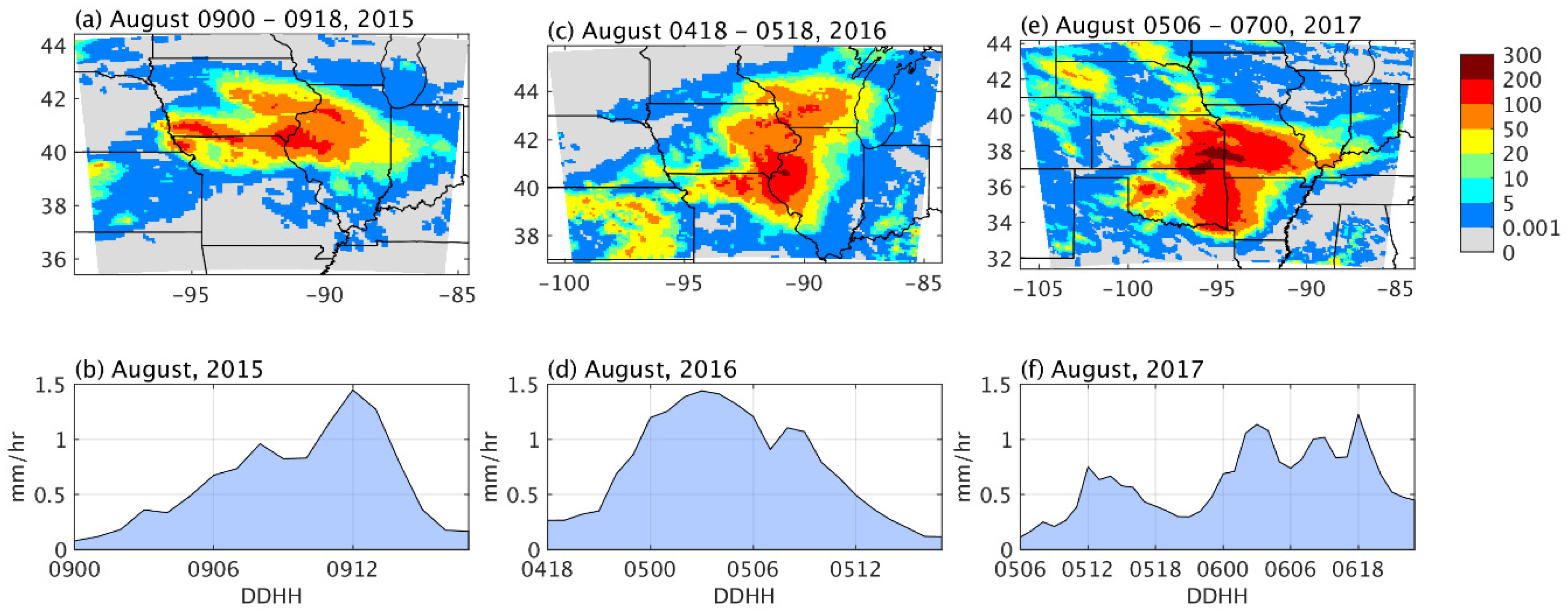
This study examines three synoptic-scale convective events over the central United States. The first event lasted 18 h and occurred on August 9, 2015; the second event lasted 24 h from 1800 UTC August 4 to 1800 UTC August 5, 2016; and the third event lasted 36 h from 0600 UTC August 5 to 0000 UTC August 7, 2017. Figure 1 shows the spatial distribution of total precipitation and the time series of domain-mean hourly precipitation for each event. The first event was a diurnal precipitation event, the second was a nocturnal precipitation event, and the third was a mixed diurnal and nocturnal event. The mechanism for diurnal precipitation is deep convection due to surface heat and moisture flux, while that for nocturnal precipitation is likely large-scale upward motion and moisture advection [30]. The three events had different spatial coverage but similar precipitation intensity. The precipitation data are linearly interpolated onto the grids used by the WRF model (see Section 2.3) using the griddata function provided by Matlab. We assimilate only the upper-left three grids of every 2-by-2 grid in the WRFDA system, that is, 75% of the observations are used in the WRFDA system, and the remaining 25% are used as independent observations when computing statistical metrics.
2.3. Model Configurations
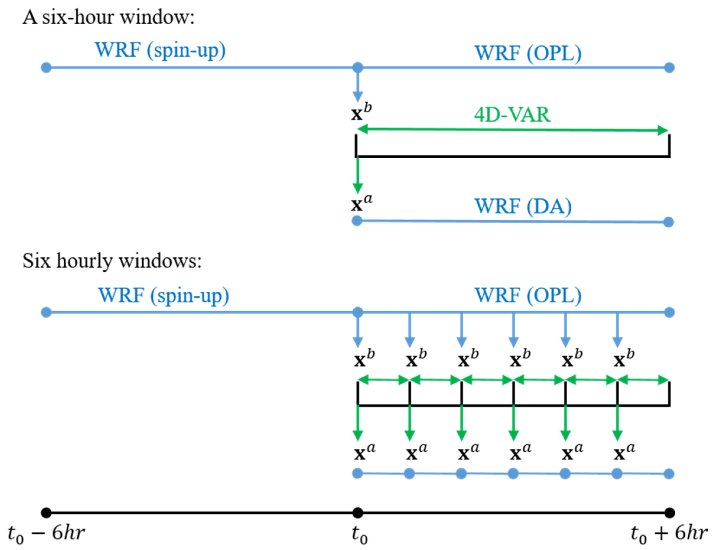
For each event, the WRF model is configured with a single domain with horizontal grid spacing of 10 km in the Lambert projection, and 30 vertical levels extending from the surface to 50 hPa. The physics options follow the physics suite for the continental United States [31] except the microphysics and cumulus schemes that are currently incompatible with the tangent linear and adjoint models. The physics schemes include the WRF single-moment 5-class microphysics [32], the Rapid Radiative Transfer Model-Global (RRTMG) for shortwave and longwave radiation [33], the unified Noah land-surface model [34], the Eta similarity scheme for the surface layer [35,36,37,38], the Mellor-Yamada-Janjic planetary boundary layer [36], and the Kain–Fritsch cumulus scheme [39]. The initial and lateral boundary conditions are from the NCEP final analysis (FNL) with a spatial resolution of 0.25° × 0.25° and a time resolution of every 6 h [40]. The WRF simulations are conducted every 6 h (i.e., = 2015-08-09-0000 UTC, = 2015-08-09-0600 UTC, etc.; Figure 2). Each simulation runs 12 h with the first 6 h being spin ups and the last 6 h being warm-start estimations (Figure 2). For the last 6 h of the simulations, we output hourly precipitation data as open loop estimates (OPL), and hourly meteorological data as the initial conditions () for assimilations (Figure 2). The error covariance of the initial conditions () is estimated through the National Meteorological Center (NMC) method embedded in the WRFDA system.
2.4. Experiments Design and Evaluation Metrics
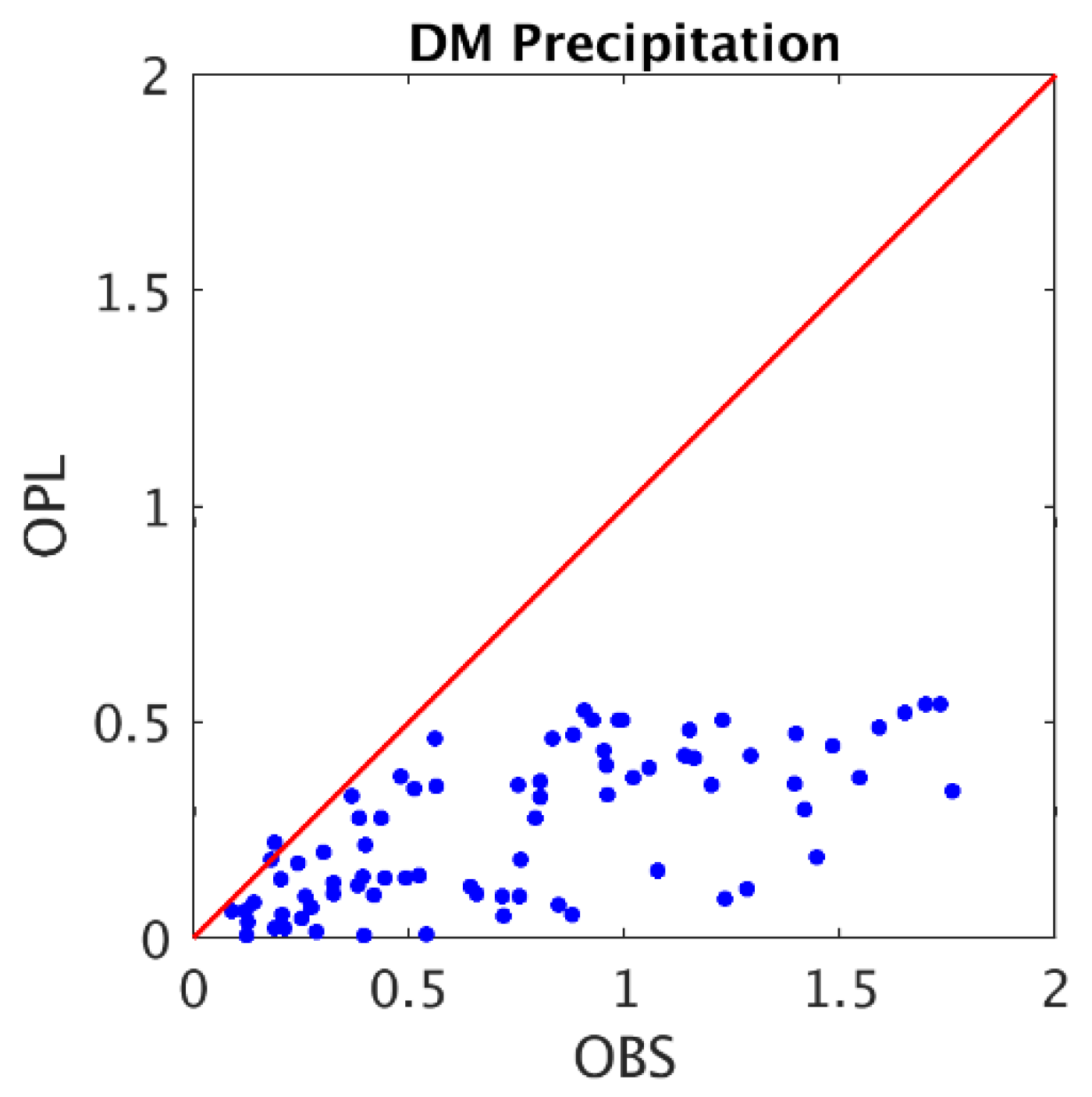
Figure 3 is a scatter plot of hourly domain-mean precipitation from OPL estimates and those from the IMERG observations for the three precipitation events. It shows that the WRF model underestimates the domain-mean precipitation for nearly all the 78 h we studied, which agrees with previous studies that show the limitations of numerical prediction models in estimating summer convective precipitation [41,42]. To find an appropriate way to assimilate the IMERG observations into the WRF 4D-Var system, we conducted five assimilation experiments, i.e., six-hour (EXP1) and hourly (EXP2) assimilation windows (Figure 2), nontransformed (EXP2) and logarithmically transformed observations (EXP3), and a different observation error for the nontransformed and logarithmically transformed observations (EXP4 and EXP5). The setups of the five experiments are listed in Table 1. To evaluate precipitation estimates from the experiments, we applied several statistical metrics, including the bias, the mean absolute difference (MAD), the correlation coefficient (CC), the probability of detection (POD), the false alarm ratio (FAR), and the Equitable Threat Score (ETS). The equation and the perfect value of each metric are listed in Table 2.
3. Results
3.1. Evaluation of Precipitation Estimates from Six-Hour-Window and Hourly-Window Experiments
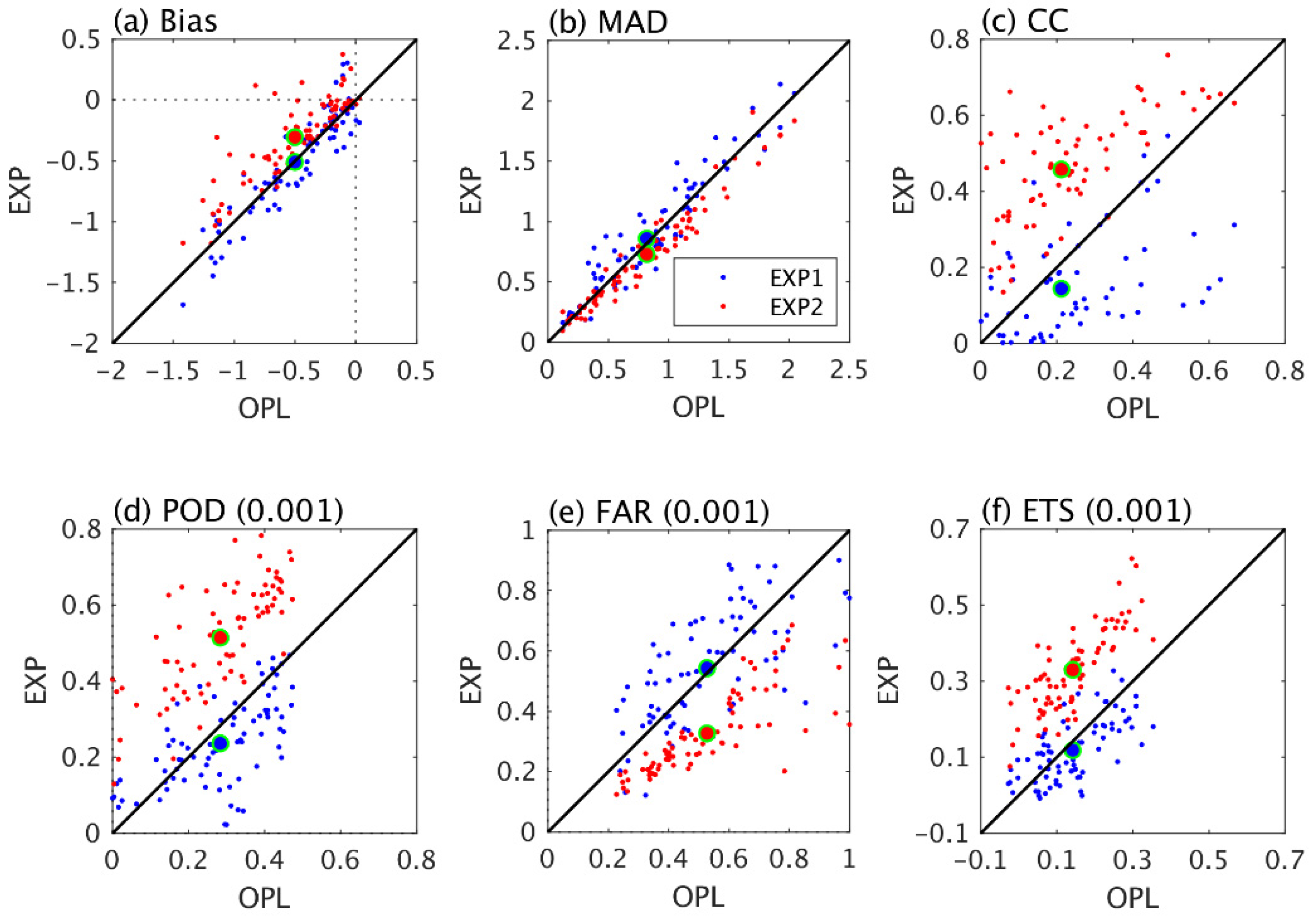
Figure 4 shows scatter plots of the statistical metrics of hourly estimates of the three events from the six-hour-window experiment (EXP1)/hourly-window experiment (EXP2) and those from the OPL experiment. Both EXP1 and EXP2 underestimate hourly precipitation for most of the hours, but the underestimations from EXP2 are smaller than those from EXP1 and those from the OPL experiment (Figure 4a). EXP1 shows slightly larger MADs and FARs and smaller CCs, PODs, and ETSs compared with the OPL experiment. In contrast, EXP2 shows slightly smaller MADs, significantly smaller FARs, and significantly higher CCs, PODs, and ETSs compared with the OPL experiment, suggesting that hourly assimilation windows improve hourly precipitation estimates better than six-hour windows do. We also looked at the statistical metrics of six-hour accumulated precipitation estimates from the two assimilation experiments and the OPL experiment (Figures not shown); the results were similar to those of hourly estimates and further suggest that the hourly windows have better performance than six-hour windows. The high performance of hourly window experiments could be partially due to the shorter integration length, which involves fewer uncertainties.
3.2. Evaluation of Precipitation Estimates from Nontransformed and Logarithmically Transformed Experiments
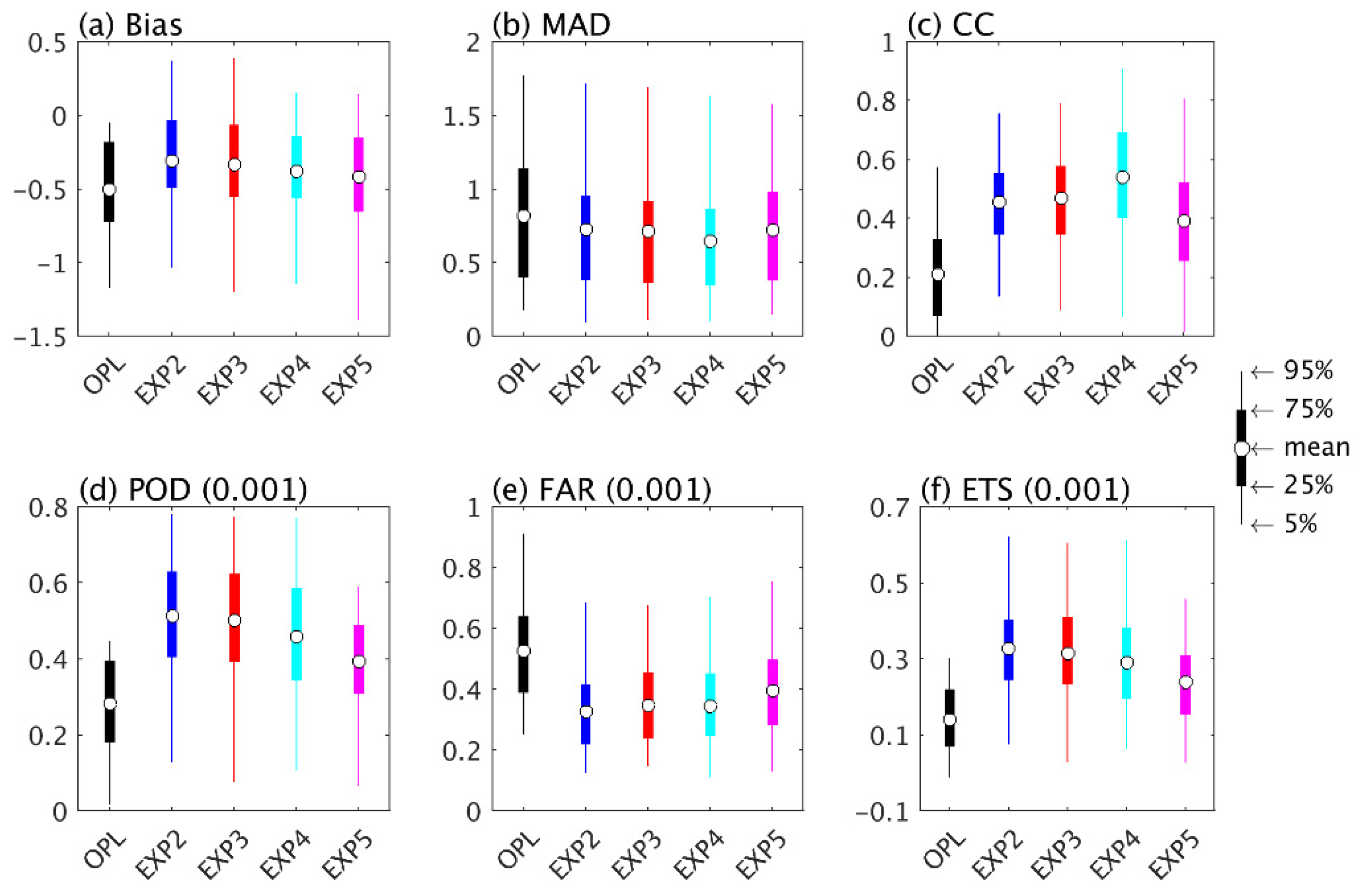
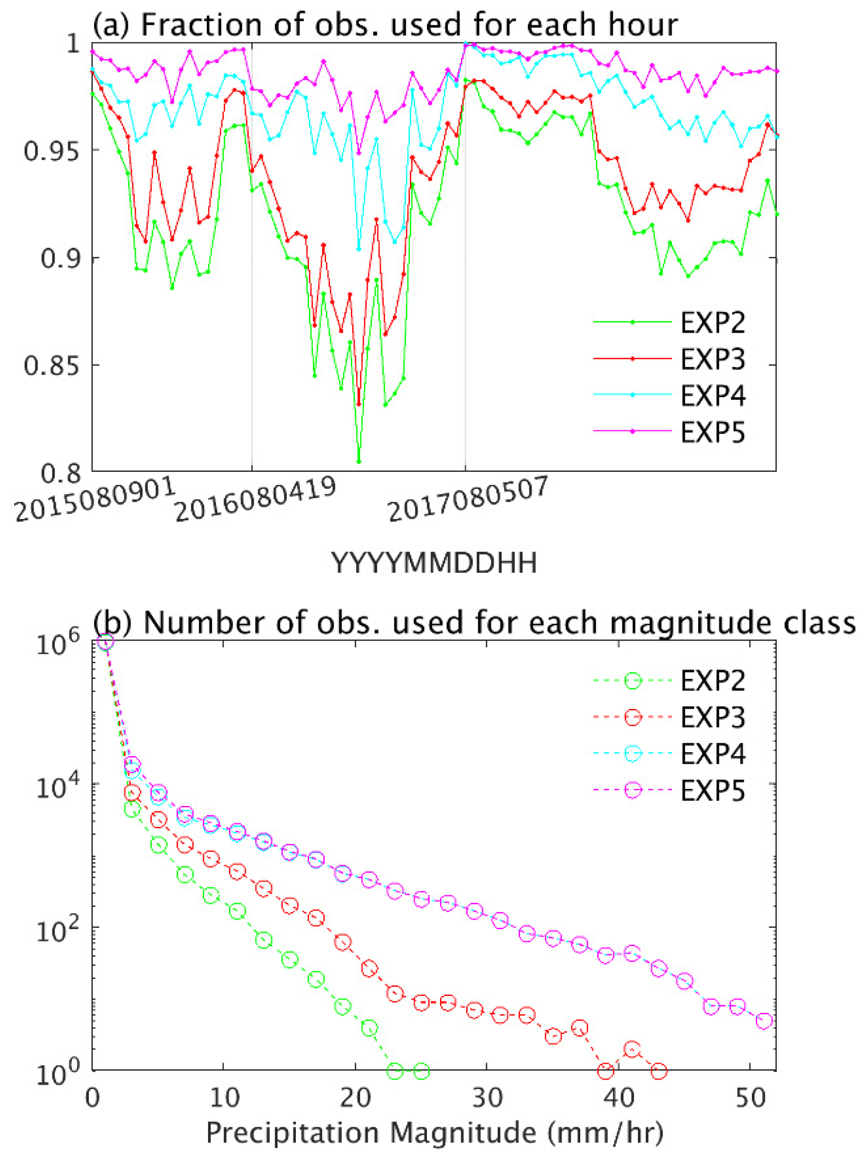
Figure 5 shows the statistical metrics (the threshold for POD, FAR, and ETS is 0.001 mm/h) of experiments of nontransformed/logarithmically transformed observations with a constant observation error in regular space (EXP2/EXP3) or in the logarithmic space (EXP4/EXP5). The figure reveals that all of these assimilation experiments showed better performance than the OPL experiment, and that the differences among the assimilation experiments were small. However, the detection scores (POD, FAR, and ETS) for each threshold (Figure 6) revealed differences among the experiments. The POD and ETS decreased and the FAR increased with the threshold. For the experiments with a constant observation error in the regular space (EXP2 and EXP3), logarithmically transformed precipitation (EXP3) showed similar performance to the nontransformed precipitation, except that the FARs of EXP3 were slightly lower when the threshold fell between 5 mm/h and 25 mm/h. This slight improvement of FARs of EXP3 was likely due to more observations being used in EXP3 compared to EXP2 (Figure 7b). For the experiments with a constant observation error in the logarithmic space (EXP4 and EXP5), nontransformed precipitation (EXP4) showed significantly lower FARs than the logarithmically transformed precipitation (EXP5), and EXP4 showed higher PODs and ETSs than EXP5 when the threshold was less than 15 mm/h and vice versa. EXP5 used more observations than EXP4 (Figure 7), but it did not yield better performance in this case, suggesting that logarithmic transformation on precipitation is not an effective way of assimilating precipitation.
A constant error in the logarithmic space () corresponds to a linearly increasing error in the regular space (Equation (6)). On one hand, the linearly increasing error modifies the threshold of rejecting observations (Equations (3) and (8)), using more observations (especially heavy precipitations) that are rejected in the experiments with a constant error in the regular space (Figure 7). On the other hand, the relative error—defined as the ratio of the precipitation error to the precipitation intensity—decreases with intensity, which means that heavy precipitation observations are more reliable than light precipitation observations in the assimilation processes. Therefore, the linearly increasing error of observations improves the detection skill (especially the detection for heavy precipitation) of the assimilation system, regardless of whether nontransformed precipitation (EXP2 and EXP4) or logarithmically transformed precipitation (EXP3 and EXP5) observations (Figure 6) are used.
4. Discussion
Based on three summer convective events over the central United States, this study evaluated the effect of assimilating IMERG precipitation into the 4D-Var WRFDA system with several experiments. The improvement of precipitation estimates varied with each experiment. We found that the 4D-Var method with hourly windows improved the precipitation estimates significantly more than that with six-hour windows. Then, we assimilated logarithmically transformed precipitation and nontransformed precipitation into the 4D-Var WRFDA system with hourly assimilation windows. Statistical metrics revealed that logarithmically transformed precipitation does not improve the precipitation estimates compared with nontransformed precipitation. This implies that the non-Gaussian structure of observation error may not be a problem for 4D-Var precipitation assimilation. Another advantage of logarithmic transformation—utilizing more observations in the assimilation process by modifying the threshold of rejecting observations—can be achieved by changing the error of observations in the 4D-Var WRFDA system with nontransformed observations (as in EXP4). Therefore, it was shown that the WRF 4D-Var method with logarithmically transformed precipitation is not a superior method of assimilating the IMERG precipitation observations compared with the regular 4D-Var method. However, this study is based on only one setting of WRF parameterizations, and the results may vary with different settings; hence, we provide the 4D-Var method with logarithmically transformed precipitation observations for future investigations.
Author Contributions
Conceptualization, J.Z., L.-F.L. and R.L.B.; methodology, J.Z., L.-F.L. and R.L.B.; software, J.Z.; validation, J.Z., L.-F.L. and R.L.B.; formal analysis, J.Z.; investigation, J.Z. and L.-F.L.; resources, J.Z.; data curation, J.Z.; writing—original draft preparation, J.Z.; writing—review and editing, L.-F.L. and R.L.B.; visualization, J.Z.; supervision, R.L.B.; project administration, R.L.B.; funding acquisition, R.L.B. All authors have read and agreed to the published version of the manuscript.
Funding
This research was funded by NASA PMM science program, grant number NNX16AE36G.
Acknowledgments
Models and data are obtained from NCAR. We would like to thank Zhiquan Liu for providing help on the logarithmic transformation for the cost function of the 4D-Var method.
Conflicts of Interest
The authors declare no conflict of interest.
Appendix A
Appling natural logarithmic transformation () on precipitation gives the following cost function:
The precipitation error covariance after transformation () is calculated as follows:
Applying Taylor expansion of at and keeping the first two terms gives
The incremental expression of the transformed cost function is organized as follows:
where is the increment relative to the first guess . Taylor expansion of at is
where , and are the tangent linear version of , and at , respectively. Keeping the first two terms of Equation (A5) and substituting it into Equation (A4) gives the transformed incremental cost function:
where .
References
- Vidale, P.L.; Luthi, D.; Frei, C.; Seneviratne, S.I.; Schar, C. Predictability and uncertainty in a regional climate model. J. Geophys. Res. 2003, 108, 4586. [Google Scholar] [CrossRef]
- Roberts, N.M. Assessing the spatial and temporal variation in the skill of precipitation forecasts from an NWP model. Meteorol. Appl. 2008, 15, 163–169. [Google Scholar] [CrossRef] [Green Version]
- Slingo, J.; Palmer, T. Uncertainty in weather and climate prediction. Philos. Trans. R. Soc. A 2011, 369, 4751–4767. [Google Scholar] [CrossRef]
- Robinson, A.R.; Lermusiaux, P.F.J. Data assimilation in models. In Encyclopedia of Ocean Sciences; Academic Press: Cambridge, MA, USA, 2001; pp. 623–634. [Google Scholar]
- Kalnay, E. Atmospheric Modeling, Data Assimilation and Predictability; Cambridge University Press: New York, NY, USA, 2003; p. 369. [Google Scholar] [CrossRef]
- Zupanski, D.; Mesinger, F. Four-dimensional variational assimilation of precipitation data. Mon. Weather Rev. 1995, 123, 1112–1127. [Google Scholar] [CrossRef] [Green Version]
- Tsuyuki, T. Variational data assimilation in the tropics using precipitation data. Part III: Assimilation of SSM/I precipitation rates. Mon. Weather Rev. 1997, 125, 1447–1464. [Google Scholar] [CrossRef]
- Koizumi, K.; Ishikawa, Y.; Tsuyuki, T. Assimilation of precipitation data to the JMA mesoscale model with a four-dimensional variational method and its impact on precipitation forecasts. SOLA 2005, 1, 45–48. [Google Scholar] [CrossRef] [Green Version]
- Lopez, P. Direct 4D-Var assimilation of NCEP Stage IV radar and gauge precipitation data at ECMWF. Mon. Weather Rev. 2011, 139, 2098–2116. [Google Scholar] [CrossRef]
- Lin, L.-F.; Ebtehaj, A.M.; Bras, R.L.; Flores, A.N.; Wang, J. Dynamical precipitation downscaling for hydrologic applications using WRF 4D-Var data assimilation: Implications for GPM era. J. Hydrometeorol. 2015, 16, 811–829. [Google Scholar] [CrossRef] [Green Version]
- Lin, L.-F.; Ebtehaj, A.M.; Flores, A.N.; Bastola, S.; Bras, R.L. Combined assimilation of satellite precipitation and soil moisture: A case study using TRMM and SMOS data. Mon. Weather Rev. 2017, 145, 4997–5014. [Google Scholar] [CrossRef]
- Ban, J.; Liu, Z.; Zhang, X.; Huang, X.-Y.; Wang, H. Precipitation data assimilation in WRFDA 4D-Var: Implementation and application to convection permitting forecasts over United States. Tellus A Dyn. Meteorol. Oceanogrol. 2017, 69, 1368310. [Google Scholar] [CrossRef] [Green Version]
- Yi, L.; Zhang, W.; Wang, K. Evaluation of heavy precipitation simulated by the WRF model using 4D-Var data assimilation with TRMM 3B42 and GPM IMERG over the Huaihe River basin, China. Remote Sens. 2018, 10, 646. [Google Scholar] [CrossRef] [Green Version]
- Gebremichael, M.; Krajewski, W.F. Modeling distribution of temporal sampling errors in area–time-averaged rainfall estimates. Atmos. Res. 2005, 73, 243–259. [Google Scholar] [CrossRef]
- Lien, G.-Y.; Kalnay, E.; Miyoshi, T.; Huffman, G.J. Statistical properties of global precipitation in the NCEP GFS model and TMPA observations for data assimilation. Mon. Weather Rev. 2016, 144, 663–679. [Google Scholar] [CrossRef] [Green Version]
- Lien, G.-Y.; Miyoshi, T.; Kalney, E. Assimilation of TRMM multisatellite precipitation analysis with a low-resolution NCEP Global Forecast System. Mon. Weather Rev. 2016, 144, 643–662. [Google Scholar] [CrossRef]
- Kneifel, S.; Löhnert, U.; Battaglia, A.; Crewell, S.; Siebler, D. Snow scattering signals in ground-based passive microwave radiometer measurements. J. Geophys. Res. Atmos. 2010, 115, D16214. [Google Scholar] [CrossRef] [Green Version]
- Levizzani, V.; Laviola, S.; Cattani, E. Detection and measurement of snowfall from space. Remote Sens. 2011, 3, 145–166. [Google Scholar] [CrossRef] [Green Version]
- Hou, A.Y.; Kakar, R.K.; Neeck, S.; Azarbarzin, A.A.; Kummerow, C.D.; Kojima, M.; Oki, R.; Nakamura, K.; Iguchi, T. The Global Precipitation Measurement Mission. Bull. Am. Meteorol. Soc. 2014, 95, 701–722. [Google Scholar] [CrossRef]
- Liu, Z.; Ostrenga, D.; Vollmer, B.; Deshong, B.; Macritchie, K.; Greene, M.; Kempler, S. Global Precipitation Measurement mission products and services at the NASA GES DISC. Bull. Am. Meteorol. Soc. 2017, 98, 437–444. [Google Scholar] [CrossRef]
- Tan, J.; Petersen, W.A.; Tokay, A. A novel approach to identify sources of errors in IMERG for GPM ground validation. J. Hydrometeorol. 2016, 17, 2477–2491. [Google Scholar] [CrossRef]
- Tang, G.; Ma, Y.; Long, D.; Zhong, L.; Hong, Y. Evaluation of GPM Day-1 IMERG and TMPA version-7 legacy over mainland China at multiple spatiotemporal scales. J. Hydrol. 2016, 533, 152–167. [Google Scholar] [CrossRef]
- Tang, G.; Zeng, Z.; Long, D.; Guo, X.; Yong, B.; Zhang, W.; Hong, Y. Statistical and hydrological comparisons between TRMM and GPM Level-3 products over a midlatitude basin: Is Day-1 IMERG a good successor for TMPA 3B42V7? J. Hydrometeorol. 2016, 17, 121–137. [Google Scholar] [CrossRef]
- O, S.; Foelsche, U.; Kirchengast, G.; Fuchsberger, J.; Tan, J.; Petersen, W.A. Evaluation of GPM IMERG early, late, and final rainfall estimates with WegenerNet gauge data in southeast Austria. Hydrol. Earth Syst. Sci. Discuss. 2017, 21, 6559–6572. [Google Scholar] [CrossRef] [Green Version]
- Huang, X.-Y.; Xiao, Q.; Barker, D.M.; Zhang, X.; Michalakes, J.; Huang, W.; Henderson, T.; Bray, J.; Chen, Y.; Ma, Z.; et al. Four-dimensional variational data assimilation for WRF: Formulation and preliminary results. Mon. Weather Rev. 2009, 137, 299–314. [Google Scholar] [CrossRef] [Green Version]
- Courtier, P.; Thepaut, J.-N.; Hollingsworth, A. A strategy for operational implementation of 4D-Var, using an incremental approach. Q. J. R. Meteorol. Soc. 1994, 120, 1367–1387. [Google Scholar] [CrossRef]
- Errico, R.M.; Fillion, L.; Nychka, D.; Lu, Z.Q. Some statistical considerations associated with the data assimilation of precipitation observations. Q. J. R. Meteorol. Soc. 2000, 126, 339–359. [Google Scholar] [CrossRef]
- Huffman, G.J.; Bolvin, D.T.; Braithwaite, D.; Hsu, K.; Joyce, R.; Kidd, C.; Nelkin, E.J.; Xie, S. NASA Global Precipitation Measurement (GPM) Integrated Multi-Satellite Retrievals for GPM (IMERG). Algorithm Theoretical Basis Document (ATBD). Version 4.5; 2015; 30p. Available online: https://pmm.nasa.gov/sites/default/files/document_files/IMERG_ATBD_V4.5.pdf (accessed on 31 March 2017).
- Huffman, G.J.; Bolvin, D.T.; Braithwaite, D.; Hsu, K.; Joyce, R.; Kidd, C.; Nelkin, E.J.; Sorooshian, S.; Stocker, E.F.; Tan, J.; et al. Integrated Multi-satellitE Retrievals for the Global Precipitation Measurement (GPM) mission (IMERG). Adv. Glob. Chang. Res. 2020, 67, 343–353. [Google Scholar]
- Lee, M.-I.; Choi, I.; Tao, W.-K.; Schubert, S.D.; Kang, I.-S. Mechanisms of diurnal precipitation over the US Great Plains: A cloud resolving model perspective. Clim. Dyn. 2009, 34, 419–437. [Google Scholar] [CrossRef]
- NCAR. Convection-Permitting Physics Suite for WRF. Available online: https://www2.mmm.ucar.edu/wrf/users/ncar_convection_suite.php (accessed on 13 June 2020).
- Hong, S.-Y.; Dudhia, J.; Chen, S.-H. A revised approach to ice microphysical processes for the bulk parameterization of clouds and precipitation. Mon. Weather Rev. 2004, 132, 103–120. [Google Scholar] [CrossRef]
- Iacono, M.J.; Delamere, J.S.; Mlawer, E.J.; Shephard, M.W.; Clough, S.A.; Collins, W.D. Radiative forcing by long–lived greenhouse gases: Calculations with the AER radiative transfer models. J. Geophys. Res. 2008, 113, D13103. [Google Scholar] [CrossRef]
- Tewari, M.; Chen, F.; Wang, W.; Dudhia, J.; LeMone, M.A.; Mitchell, K.; Ek, M.; Gayno, G.; Wegiel, J.; Cuenca, R.H. Implementation and verification of the unified NOAH land surface model in the WRF model. In Proceedings of the 20th Conference on Weather Analysis and Forecasting/16th Conference on Numerical Weather Prediction, Seattle, WA, USA, 10–15 January 2004; American Meteorological Society: Boston, MA, USA, 2004; pp. 11–15. Available online: https://ams.confex.com/ams/84Annual/techprogram/paper_69061.htm (accessed on 12 June 2017).
- Monin, A.S.; Obukhov, A.M. Basic laws of turbulent mixing in the surface layer of the atmosphere. Contrib. Geophys. Inst. Acad. Sci. USSR 1954, 151, 163–187. (In Russian) [Google Scholar]
- Janjic, Z.I. The step-mountain Eta coordinate model: Further developments of the convection, viscous sublayer and turbulence closure schemes. Mon. Weather Rev. 1994, 122, 927–945. [Google Scholar] [CrossRef] [Green Version]
- Janjic, Z.I. The surface layer in the NCEP Eta Model. In Proceedings of the Eleventh Conference on Numerical Weather Prediction, Norfolk, VA, USA, 19–23 August 1996; American Meteorological Society: Boston, MA, USA, 1996; pp. 354–355. Available online: https://www2.mmm.ucar.edu/wrf/users/phys_refs/SURFACE_LAYER/eta_part3.pdf (accessed on 12 June 2017).
- Janjic, Z.I. Nonsingular Implementation of the Mellor-Yamada Level 2.5 Scheme in the NCEP Meso Model; NCEP Office Note No. 437; NCEP: College Park, MD, USA, 2002; p. 61. Available online: https://repository.library.noaa.gov/view/noaa/11409/noaa_11409_DS1.pdf (accessed on 12 June 2017).
- Kain, J.S. The Kain–Fritsch convective parameterization: An update. J. Appl. Meteorol. 2004, 43, 170–181. [Google Scholar] [CrossRef] [Green Version]
- National Centers for Environmental Prediction/National Weather Service/NOAA/U.S. Department of Commerce: NCEP GDAS/FNL 0.25 Degree Global Tropospheric Analyses and Forecast Grids. Research Data Archive at the National Center for Atmospheric Research, Computational and Information Systems Laboratory. 2015. Available online: https://doi.org/10.5065/D65Q4T4Z (accessed on 21 June 2017).
- Sun, J.; Xue, M.; Wilson, J.W.; Zawadzki, I.; Ballard, S.P.; Onvlee-Hooimeyer, J.; Joe, P.; Barker, D.M.; Li, P.-W.; Golding, B.; et al. Use of NWP for nowcasting convective precipitation: Recent progress and challenges. Bull. Am. Meteorol. Soc. 2014, 95, 409–426. [Google Scholar] [CrossRef] [Green Version]
- Zhang, J.; Lin, L.-F.; Bras, R.L. Evaluation of the quality of precipitation products: A case study using WRF and IMERG data over the central United States. J. Hydrometeorol. 2018, 19, 2007–2020. [Google Scholar] [CrossRef]
Figure 1.
The three precipitation events studied in this paper. (a) The spatial distribution of total precipitation amount and (b) the time series of hourly domain-mean precipitation during 0000–1800 UTC August 9, 2015. Figure sets (c–f) are as for (a,b), but for precipitation during 1800 UTC August 4–1800 UTC August 5, 2016 and 0600 UTC August 5–0000 UTC 7 August 2017, respectively.

Figure 2.
The steps of running open loop (OPL) and data assimilation (DA) experiments with hourly and six-hour assimilation windows.
Figure 2.
The steps of running open loop (OPL) and data assimilation (DA) experiments with hourly and six-hour assimilation windows.

Figure 3.
Scatter plot of hourly domain-mean observed precipitation and open-loop estimated precipitation (mm/h).
Figure 3.
Scatter plot of hourly domain-mean observed precipitation and open-loop estimated precipitation (mm/h).

Figure 4.
Scatter plot of the statistics of hourly domain-mean precipitation (mm/h) from WRFDA experiments against that from the open-loop experiment. The circles with green edges represent mean values.
Figure 4.
Scatter plot of the statistics of hourly domain-mean precipitation (mm/h) from WRFDA experiments against that from the open-loop experiment. The circles with green edges represent mean values.

Figure 5.
Boxplots of statistical metrics of hourly precipitation estimates estimated from each assimilation experiment and the OPL experiment. The threshold for calculating the POD, FAR, and ETS is 0.001 mm/h, which is the threshold of distinguishing precipitation or no precipitation in the IMERG data. EXP2 and EXP3 represent experiments with nontransformed and logarithmically transformed precipitation with constant observation error, respectively; EXP4 and EXP5 are as for EXP2 and EXP3, but with increasing observation error with precipitation magnitude.

Figure 6.
Detection scores of hourly precipitation estimated from assimilation experiments and the OPL experiment at different thresholds ranging from 1 mm/h to 30 mm/h. EXP2 and EXP3 represent experiments with nontransformed and logarithmically transformed precipitation with constant observation error, respectively; EXP4 and EXP5 are as for EXP2 and EXP3, but with increasing observation error with precipitation magnitude.

Figure 7.
(a) Fraction of observations used in each assimilation experiment to the total available observations at each hour. (b) Number of observations used for all the hours at different magnitude classes with 1 mm/h intervals. EXP2 and EXP3 represent experiments with nontransformed and logarithmically transformed precipitation with constant observation error, respectively; EXP4 and EXP5 are as for EXP2 and EXP3, but with increasing observation error with precipitation magnitude.


Table 1.
Experimental setup used in this study.
| Experiment Name | Assimilation Window | Transformation of Precipitation | Errors in Regular Space (mm/h) | Errors in Log Space (mm/h) |
|---|---|---|---|---|
| EXP1 | 6-hour | No transformation | 2 (mm/6 h) | -- |
| EXP2 | Hourly | No transformation | 0.3 | 0.3/(yi + 1) |
| EXP3 | Hourly | Log transformation | 0.3 | 0.3/(yi + 1) |
| EXP4 | Hourly | No transformation | 0.3 × (yi + 1) | 0.3 |
| EXP5 | Hourly | Log transformation | 0.3 × (yi + 1) | 0.3 |
Table 2.
Statistical metrics used in this study 1.
| Statistical Metrics | Equation | Perfect Value |
|---|---|---|
| Bias | Bias = Xe − Xr | 0 |
| Mean Absolute Difference (MAD) | MAD = |Xe − Xr| | 0 |
| Correlation Coefficient (CC) | CC = cov(Xe, Xr)/ (std(Xe)∙std(Xr)) | 1 |
| Probability of Detection (POD) | POD = a/(a + c) | 1 |
| False Alarm Ratio (FAR) | FAR = b/(a + b) | 0 |
| Equitable Threat Score (ETS) | ETS = (a − e)/(a + b + c − e), where e = (a + b)(a + c)/(a + b + c + d) | 1 |
1 Xe and Xr are estimates and reference, respectively. cov(Xe, Xr) is the covariance of Xe and Xr, and std(X) is the standard deviation of X. a represents the number of grids that Xr ≥ x0 and Xe ≥ x0; b represents the number of grids that Xr < x0 but Xe ≥ x0; c represents the number of grids that Xr ≥ x0 but Xe < x0; d represents the number of grids that Xr < x0 and Xe < x0; and x0 is a threshold of precipitation magnitude.
© 2020 by the authors. Licensee MDPI, Basel, Switzerland. This article is an open access article distributed under the terms and conditions of the Creative Commons Attribution (CC BY) license (http://creativecommons.org/licenses/by/4.0/).
Share and Cite
MDPI and ACS Style
Zhang, J.; Lin, L.-F.; Bras, R.L. Effect of Logarithmically Transformed IMERG Precipitation Observations in WRF 4D-Var Data Assimilation System. Water 2020, 12, 1918. https://doi.org/10.3390/w12071918
AMA Style
Zhang J, Lin L-F, Bras RL. Effect of Logarithmically Transformed IMERG Precipitation Observations in WRF 4D-Var Data Assimilation System. Water. 2020; 12(7):1918. https://doi.org/10.3390/w12071918
Chicago/Turabian StyleZhang, Jiaying, Liao-Fan Lin, and Rafael L. Bras. 2020. "Effect of Logarithmically Transformed IMERG Precipitation Observations in WRF 4D-Var Data Assimilation System" Water 12, no. 7: 1918. https://doi.org/10.3390/w12071918
Note that from the first issue of 2016, this journal uses article numbers instead of page numbers. See further details here.