High-Resolution Coherency Functionals for Improving the Velocity Analysis of Ground-Penetrating Radar Data


1
Department of Earth Sciences, University of Pisa, 56126 Pisa, Italy
2
CISUP, Centro per l’Integrazione della Strumentazione dell’Università di Pisa, 56126 Pisa, Italy
*
Author to whom correspondence should be addressed.
Remote Sens. 2020, 12(13), 2146; https://doi.org/10.3390/rs12132146
Submission received: 18 May 2020
/
Revised: 1 July 2020
/
Accepted: 1 July 2020
/
Published: 4 July 2020
(This article belongs to the Special Issue Advanced Techniques for Ground Penetrating Radar Imaging)
Abstract
:We aim at verifying whether the use of high-resolution coherency functionals could improve the signal-to-noise ratio (S/N) of Ground-Penetrating Radar data by introducing a variable and precisely picked velocity field in the migration process. After carrying out tests on synthetic data to schematically simulate the problem, assessing the types of functionals most suitable for GPR data analysis, we estimated a varying velocity field relative to a real dataset. This dataset was acquired in an archaeological area where an excavation after a GPR survey made it possible to define the position, type, and composition of the detected targets. Two functionals, the Complex Matched Coherency Measure and the Complex Matched Analysis, turned out to be effective in computing coherency maps characterized by high-resolution and strong noise rejection, where velocity picking can be done with high precision. By using the 2D velocity field thus obtained, migration algorithms performed better than in the case of constant or 1D velocity field, with satisfactory collapsing of the diffracted events and moving of the reflected energy in the correct position. The varying velocity field was estimated on different lines and used to migrate all the GPR profiles composing the survey covering the entire archaeological area. The time slices built with the migrated profiles resulted in a higher S/N than those obtained from non-migrated or migrated at constant velocity GPR profiles. The improvements are inherent to the resolution, continuity, and energy content of linear reflective areas. On the basis of our experience, we can state that the use of high-resolution coherency functionals leads to migrated GPR profiles with a high-grade of hyperbolas focusing. These profiles favor better imaging of the targets of interest, thereby allowing for a more reliable interpretation.

1. Introduction
The Ground-Penetrating Radar (GPR) method is based on electromagnetic wave (EM) propagation and its response to changes in the EM properties of the subsurface. An EM impulse (GPR wave) generated by a transmitting antenna (transmitter, TX) propagates in the subsurface and is reflected by an interface or “scatters” on a discrete object. The energy back-reflected/scattered to the surface is recorded by a receiving antenna (receiver, RX) [1,2]. The estimation of the propagation velocity field of GPR waves (hereinafter velocity field) is an important issue to obtain a reliable and focused data migration, a crucial processing step to achieve a correct final interpretation [2,3,4,5]. This is particularly true in complex subsurface contexts, where the existence of numerous and different targets (e.g., walls, voids, pavements, fractures, metal rebars, burials) interspersed in heterogeneous materials may generate several reflections and diffraction patterns. In such cases, adopting a constant velocity for migration may produce unsatisfactory results, potentially reducing the data interpretation. The subsurface contexts whose imaging may benefit from an accurate velocity field estimation are thereby numerous, from archeology to civil engineering and structural geology settings. Velocity analysis on GPR data is usually carried out using an approximate approach in which a synthetic hyperbola of known velocity is imposed on hyperbolic-shaped real data, i.e., a real diffraction evident in the GPR profile. By a visual fitting of the curvature of the synthetic hyperbola with the observed real diffraction, the GPR wave velocity is determined. Alternatively, the semblance functional [6] on a data subset extracted from the radar profile is used. These operations are performed on a point or in a selected area of the GPR profile, where the signal-to-noise ratio (S/N) of the diffractions is high. Recently, automatic tools of hyperbola detection have been introduced assisting the operators in data analysis and processing [7,8]. However, avoiding false identifications may require some manpower effort and expertise. The resulting velocity field is constant or at most varying only with depth (1D). The estimated velocity is then used for data migration, thus collapsing the diffractions and moving the observed events in the correct position on the migrated section. When a basic processing sequence is adopted the estimated velocity is frequently used just for a vertical time-to-depth conversion. This way of proceeding disregards many factors that can actually result in an inaccurate velocity field estimation, thereby not favoring the production of an optimal migrated or depth converted section. The most important of these factors is that the propagation velocity of the electromagnetic radiation can vary both vertically and laterally along the survey profile. Although in many case studies the GPR investigated medium can be approximately considered homogeneous, there are a lot of settings where this assumption is not applicable a priori, in particular where a survey covers extensive areas and the subsurface may vary for instance in terms of sediment grain-size, material density/compaction, water content, target composition, voids occurrence among the other. Another relevant issue worth mentioning is the form of the recorded event. It is commonly assumed to be an ideal point-source hyperbolic diffraction, but frequently the scatterer is not point-like but has a flat or slightly inclined top part. Thereby the recorded event can appear like a misshapen hyperbola, composed by a planar/slightly inclined reflection and one or two lateral arms. This leads to an incorrect velocity estimation caused by difficulties in fitting a synthetic hyperbola. In this case, and also when a sharp lateral target termination is present in the subsurface (e.g., the edge of wall, interruption of stratigraphic layers caused by burials) [9], it should be more appropriate to use only one arm (left or right) of the fitting hyperbola to avoid introducing significant errors in the estimated velocity.
In this study, we propose the application to GPR data of the methodology based on high-coherency functionals computation. The computation of signal coherency (the similarity of the signal between adjacent traces) according to these functionals has long been proven to be effective in seismic exploration to estimate reflection event parameters in a common midpoint gather (CMP), even in cases of low S/N [10,11,12,13,14,15,16,17,18]. Moreover, this methodology offers a higher resolution of the estimated parameters with respect to the semblance functional [6] that is frequently used in various applications, including GPR velocity analysis [3]. The technique consists of the computation of high-resolution coherency maps by means of functionals that have been adapted from a pre-stack (source and receiver location some offset apart) to a post-stack (source and receiver coincident) velocity analysis. Applying this technique to GPR data may offer an additional processing tool capable of improving the correct location and focusing of subsurface objects in GPR profiles thanks to a more accurate velocity field estimation. We apply this technique first to a synthetic radar profile to test the effectiveness of the proposed method and evidence some possible issues potentially manifesting when real data are processed. Then we estimate the velocity field on a real data set composed of 41 parallel GPR profiles acquired in an archaeological site (Badia Pozzeveri, Lucca, Italy) and migrate the data in time with a Kichhoff algorithm. The archeological site was used because there is the possibility of ground-truthing the results of GPR data processing thanks to the evidence of excavations in the same area previously covered by the survey [9]. The migrated GPR lines were used to build some time-slices, depicting spatial coherencies of reflected energy consistent with archaeological targets [19,20,21,22,23,24,25].
2. Materials and Methods
2.1. Site Description and GPR Survey
The real GPR data of this study come from the archaeological site of Badia Pozzeveri (43°49′20″N, 18°38′39″E), located about 10 km south-east of the city of Lucca (north-west Italy). Here, an 11th-century church was believed to be larger than it is today, and buried structures were expected [26]. A GPR survey was conducted with a radar system of the IDS Georadar Company [27] equipped with a monostatic transmitter and receiver that operate at 600 MHz (nominal peak frequency). A common offset acquisition of 41 parallel survey lines 50 cm-spaced was performed covering an area of about 660 m2. The in-line trace spacing of 1.2 cm was controlled by an odometer wheel. The configuration for acquisition provided 1024 samples in a time window of 100 ns (Figure 1). Previous GPR processing revealed the existence of walls buried at variable depths in the modern churchyard together with other reflective areas potentially related to anthropogenic features (e.g., tombs, burials, channels) [9]. These results found a good match with the excavation results undertaken after the GPR survey. Indeed, the excavation operation made it possible to discover the foundations and parts of the structures of the church, as well as several medieval and modern tomb features. Finally, in the area of the modern churchyard, the excavation revealed a channel for the drainage of rainwater, contained in a funnel-shaped section and originating near the entrance of the church.
2.2. High Coherency Functionals Rationale
The travel time equation of electromagnetic waves recorded at the surface from a point diffractor in a homogeneous medium is given by:
where t is travel time, x is the horizontal coordinate of the transmitting and receiving antennae, (x0,z0) the coordinates of the diffractor with the vertical axis z pointing downward, t0 = 2 z0/V the two-way travel time for x = x0 and V the velocity of the electromagnetic wave in the medium.
A common way to estimate the velocity V is to use the semblance functional (Cs) that measures the ratio between the signal energy and the total energy in a given time window that follows a predefined hyperbolic trajectory within a user-defined aperture or number of summed traces:
where (t0,Vs) are the parameters of the hyperbola, T is the window length in ns, M is the number of traces considered, di are the data of the ith trace. The semblance is known to be a robust coherency measure against noise [6]. However, the semblance coherency functional is only able to compute low-resolution panels, limiting the precision and accuracy of the estimated subsurface velocity.
In signal processing, and in particular in seismic exploration, a wide variety of tools has been developed to detect a signal that is buried in the noise [13,15,16,17]. Such tools exploit the signal coherency among different traces gathered in common midpoint gathers (CMP). Even in the CMP case, the travel time equation is hyperbolic, and thereby the techniques that have been developed can easily be adapted to the GPR velocity estimation. Due to the high number and variety of existing tools found in literature, it is not possible to comment on them all in detail here. Therefore, we only give a brief description of those, in addition to the semblance, we have found more promising in the tests we performed on GPR data in terms of resolution, noise rejection and computational time.
The first one we consider is the Complex Matched Analysis (Ccm) functional proposed by Spagnolini et al. [28]. It makes use of an approximate estimation of the wavelet to obtain a more efficient rejection of the random noise and is able to better discriminate between interfering events. The Ccm is given by:
where (t0,Vs), T, and M have the same meaning as before and Di is the ith trace data filtered in the Hilbert domain by an estimated or known wavelet. Its efficacy has been proved on seismic data also by Tognarelli et al. [17,29]; however, we expect a resolution similar to the estimated wavelet that is employed and, ultimately, to the semblance.
The second functional we consider is given by the Complex Matched Coherency Measure (Ccmcm) algorithm, originally described by Key and Smithson [11]. It exploits the high resolution that can be achieved using the eigenvalue analysis of the data covariance matrix computed in a short time window that encompasses the signal. Considering the first eigenvalue as due to the signal and the others as due to uncorrelated random noise, the S/N can be computed as:
where λi are the eigenvalues of the data covariance matrix in decreasing order of magnitude and M is the number of traces used. The computed S/N re-scaled in the [0 1] interval gives the Ccmcm measure. The resolution that is achieved with this functional is very high. However, the combined use of a complex matched filter and the eigenstructure analysis of the data covariance matrix allows for better discrimination of interfering or crossing events [17].
For this reason, a third functional has been introduced, given by a combination of the Ccmcm and Ccm algorithms, trying to benefit from the positive properties of both. In other words, the Ccmcm has been integrated with the Ccm by Grandi et al. [14,15], thus combining the robustness inherited by the Ccm with the resolution capabilities of Ccmcm. Therefore, the new functional is given by:
Overall, we tested more than 15 functionals, built on the basis of the original description given in the cited references and also obtained through their combination. Our choice has represented the best trade-off between the required characteristics of a signal coherency estimator (i.e., high resolution and noise rejection capability) and allowed us to pick the velocity spectra on GPR data with good reliability.
3. Results
3.1. Velocity Analysis of the Synthetic Data
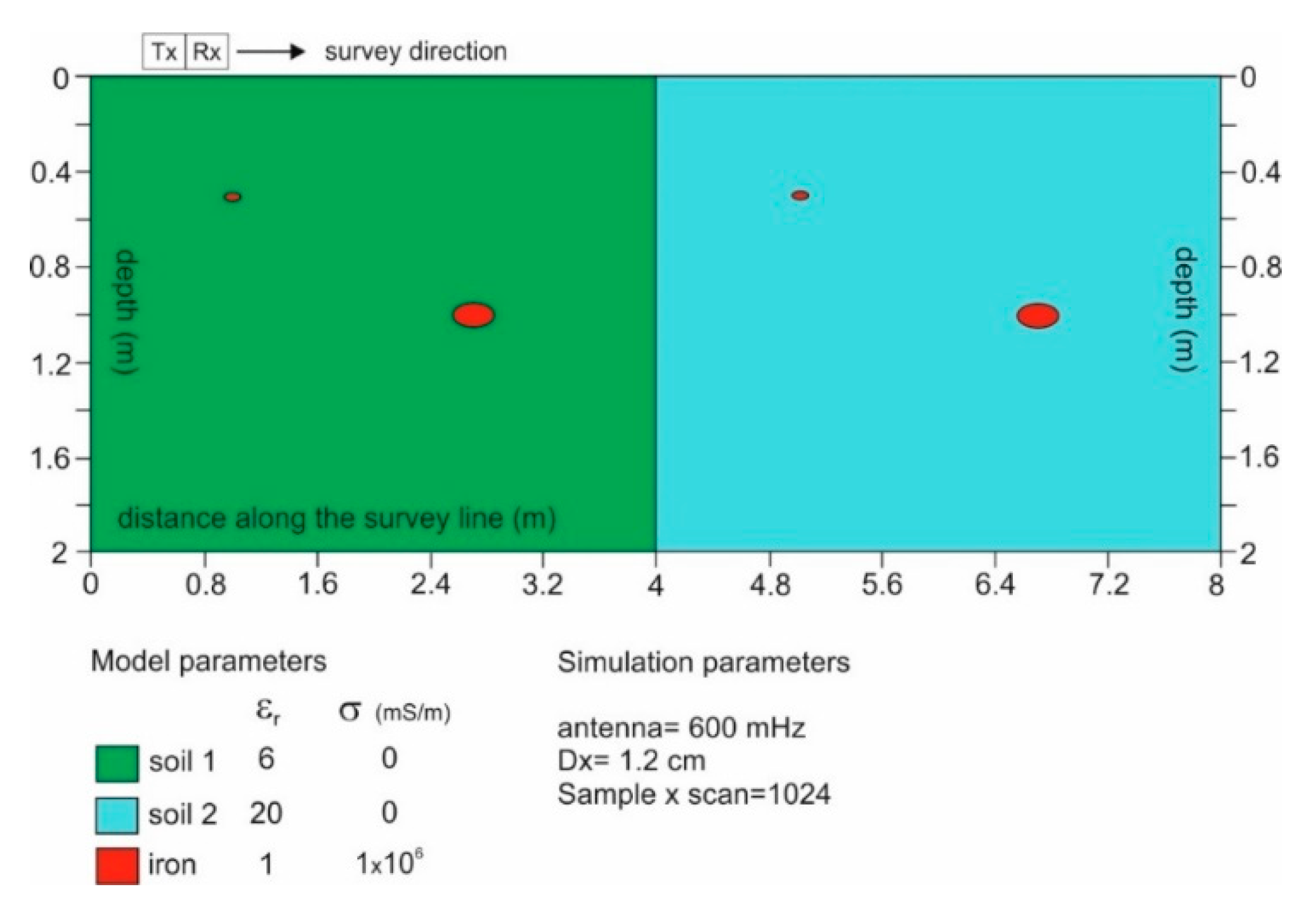
We tested the proposed methodology on a synthetic data set built by using the 2D forward modelling software GPRSIM 3.0 by Geophysical Archaeometry Laboratory [30] based on ray-tracing techniques [31]. Via a discrete grid, we built a ground model (Figure 2) composed by two regions of different relative permittivity (εr), resulting in a velocity of approximately 12.2 cm/ns and 6.7 cm/ns on the left and right sides, respectively. Inside each region, two iron objects of different sizes are placed at different depths. We run a GPR simulation according to the same parameters (antenna frequency, temporal window, sampling frequency in the spatial and temporal domains) adopted in the GPR survey composing the real dataset (see later in the text). Furthermore, and consistently with the constructive parameter of the employed GPR, we simulated a transmitter radiating GPR waves over a 170° angle (symmetrical half aperture of 85° with respect to the vertical). The impulse shape was set as Ricker wavelet, resulting in the computed radar profile shown in Figure 3. Note that in the asymptotic hyperbolic arms far away from the top of the events, some arrivals are not computed. This is due to the discretization of the grid or of the starting angles of the rays, and some arrivals are missed even if smaller discretizations than the ones used are set. However, we can consider this problem as a more severe test that mimics the absence of the signal in the velocity analysis because of missing traces. As it will be evident in the computation of the coherency spectra, the proposed methodology is solid enough to overcome this issue if it is not too severe.
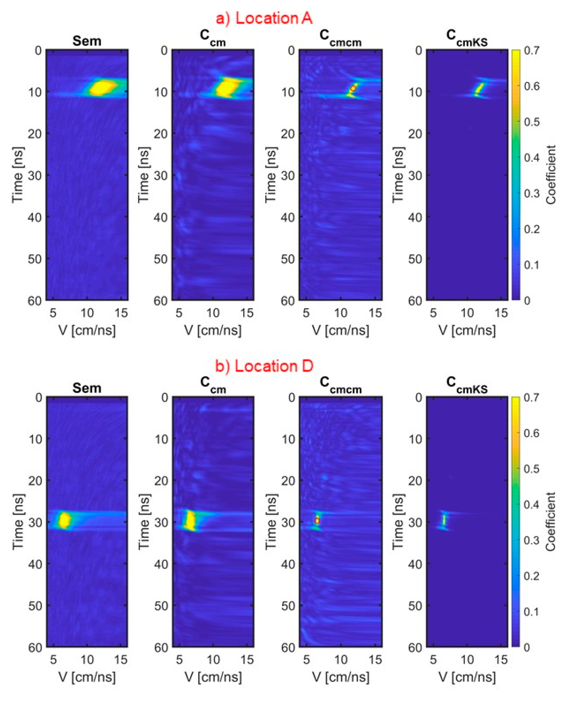
The velocity analysis using the previously-described functionals has been carried out on the events of the GPR profile in Figure 3 with the parameters illustrated in Table 1. As examples, coherency maps computed for the positions A and D are displayed in Figure 4a,b, along with the picked events marked by a red circle. Each of these (t0,Vs) pairs corresponds to the hyperbolic trajectory imposed on the GPR profile at the analysis location (hyperbola with magenta and green arms, Figure 3).
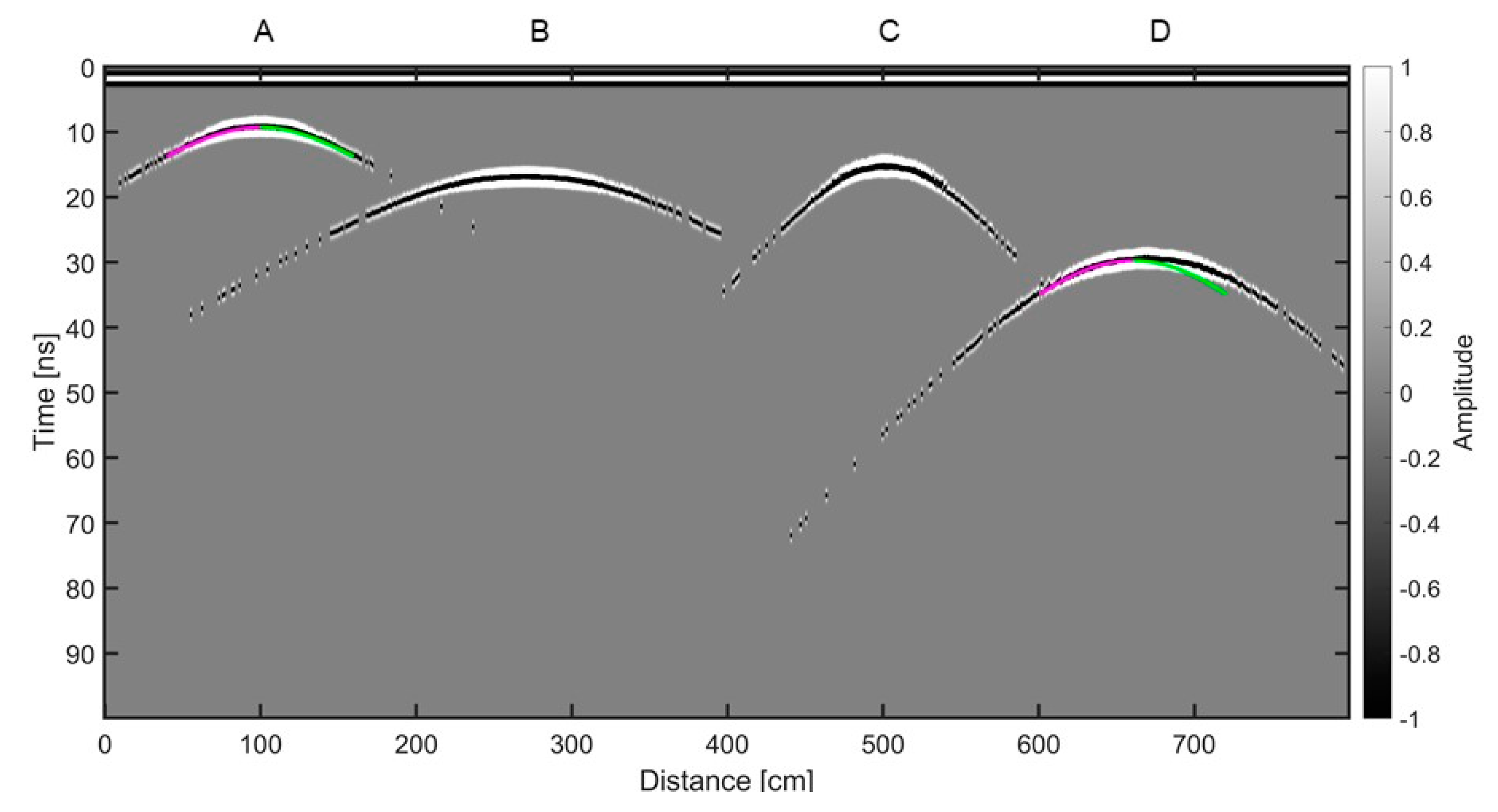
As it can be observed in Figure 4a,b, the resolution of Ccmcm and CcmKS functionals is much higher than the one given by the semblance and by Ccm, and consequently, the velocity picking is much easier and accurate. It is well worth noting that the velocity analysis described has been performed using only the portion of the data to the left of the apex (the data pertaining to the magenta hyperbola arm). The reason for this choice is that the full hyperbola does fit an event in the radargram if it originates from an object that can actually be considered a point diffractor. The object in A is sufficiently small to fulfill this requirement, as testified by the fitting of the green right arm also to the data. Instead, the dimensions of the object in D do not satisfy this point-like requirement and generate an event that differs from a classic hyperbola. Also, including in the velocity analysis the data in the correspondence of the green arm, we obtain a less accurate coherency map, and the velocity picking becomes inevitably more difficult or even impossible. For the event in A, the manual picking allows us to estimate a velocity of 11.8 cm/ns at 9.2 ns, and for the event in D a velocity of 6.6 cm/ns at 29.5 ns using the Ccmcm functional. These values are in good agreement with the background velocities given above (12.2 cm/ns and 6.7 cm/ns respectively).
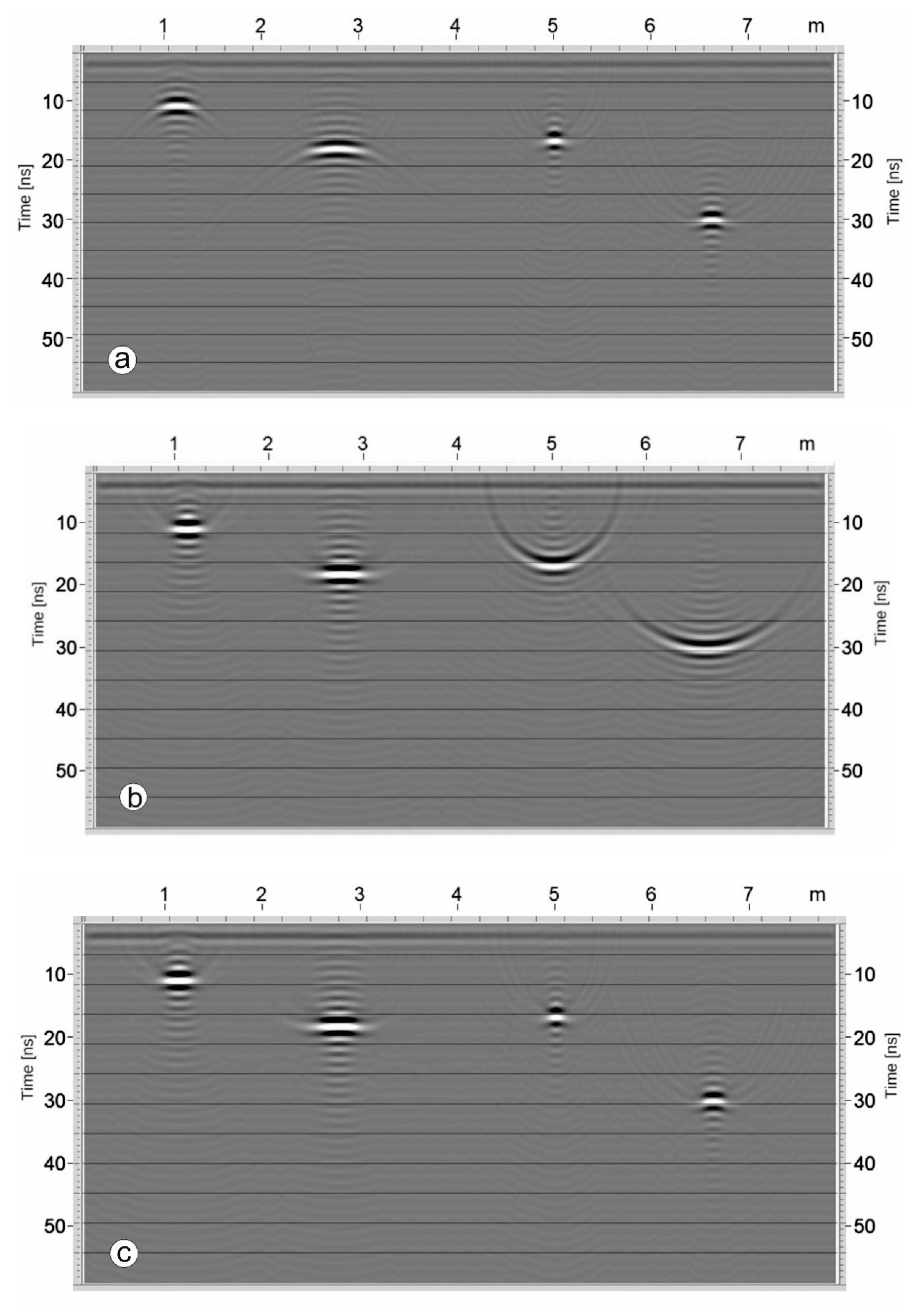
The picked (t0,Vs) pairs are used to time migrate the radar profile with a Kirchhoff algorithm [32]. Figure 5 displays in frames (a) and (b) the outcomes obtained using a constant velocity field built with the lower (6.7 cm/ns) and higher (12.2 cm/ns) velocity, respectively, and in frame (c) the outcomes when the input to migration is the varying velocity model built with the picked values (in A, B, C, and D). It is clear that only in the latter case do we have a satisfactory result from migration, and that in (a) and (b) only a portion of the radar profile is correctly migrated.
From this application of high-coherency functionals to synthetic data, it is evident that the migrated GPR profile can benefit from an accurate velocity analysis carried out both across time in a determined location and along the whole profile where hyperbolic diffractions are present.
3.2. Velocity Analysis on the Real Data
We performed the velocity analysis using the previously described functionals on data that have undergone the following processing steps to increment the S/N ratio and to reduce the reverberations: (1) background removal; (2) a band-pass filter in the range of 80-100-600-700 MHz to select only the frequencies related to the transmitted electromagnetic energy; (3) an automatic gain control on a time window of 10 ns to recover the low amplitudes of the signal at a later time; (4) a predictive deconvolution (prediction lag 2 ns, filter length 4 ns) to reduce the reverberations observed on the radargram, thus facilitating the velocity analysis; (5) a more selective band-pass filter in the range of 80-120-450-550 MHz.
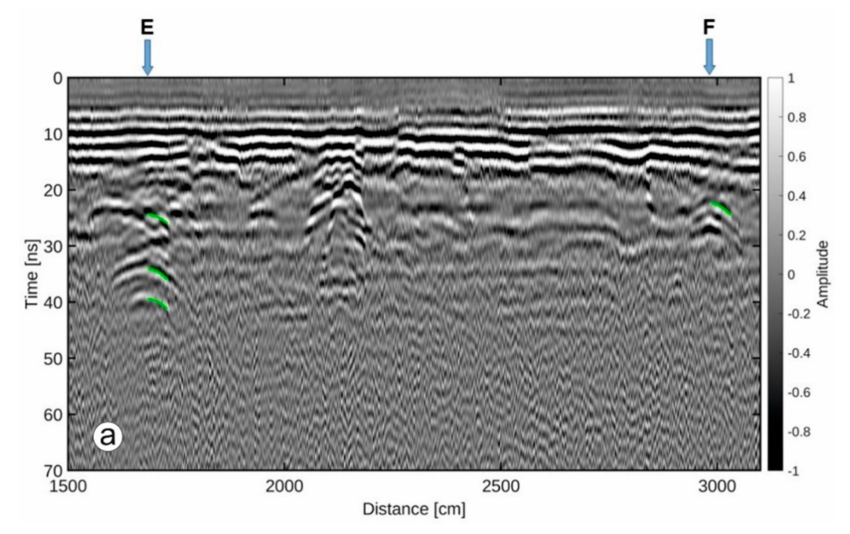
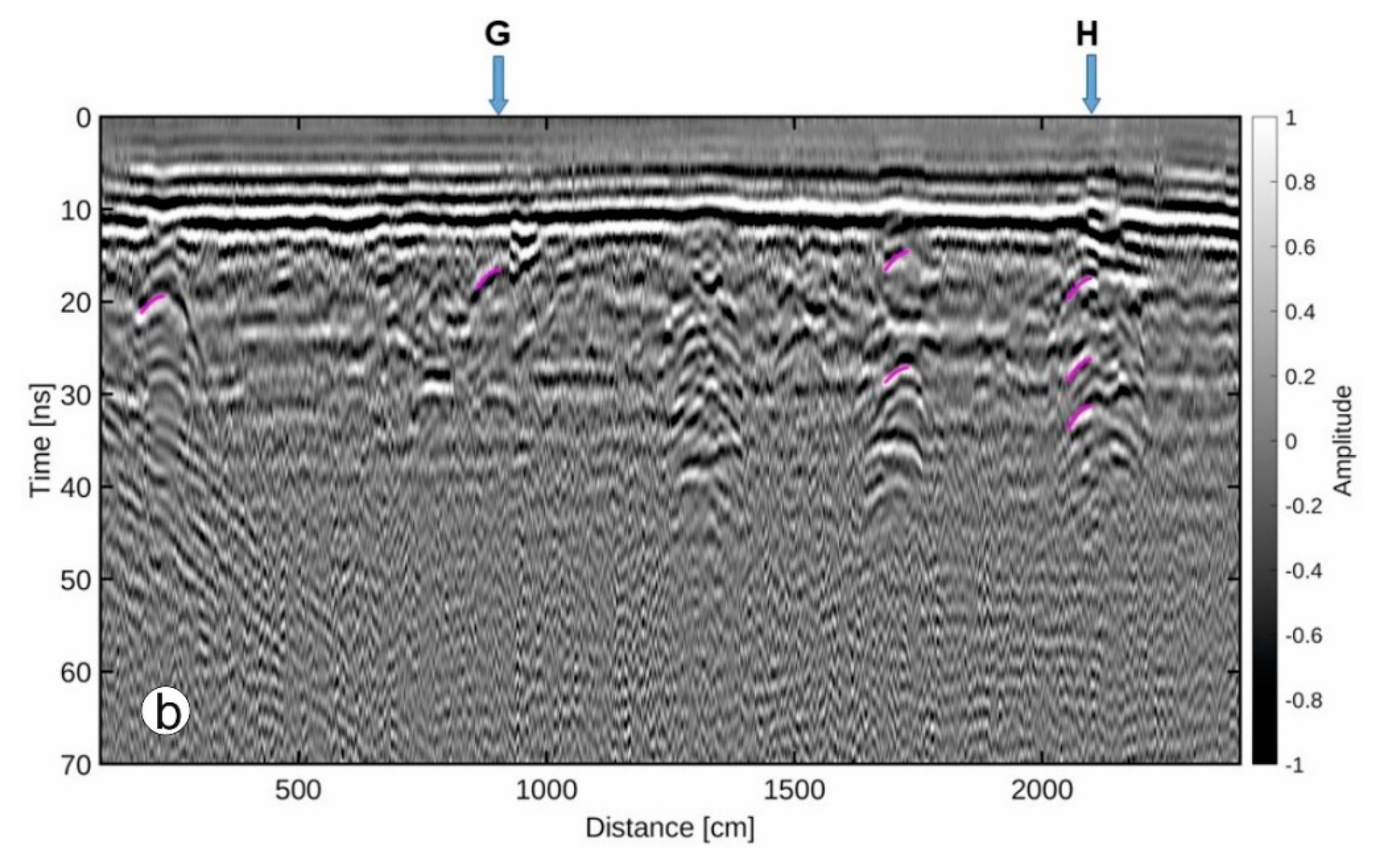
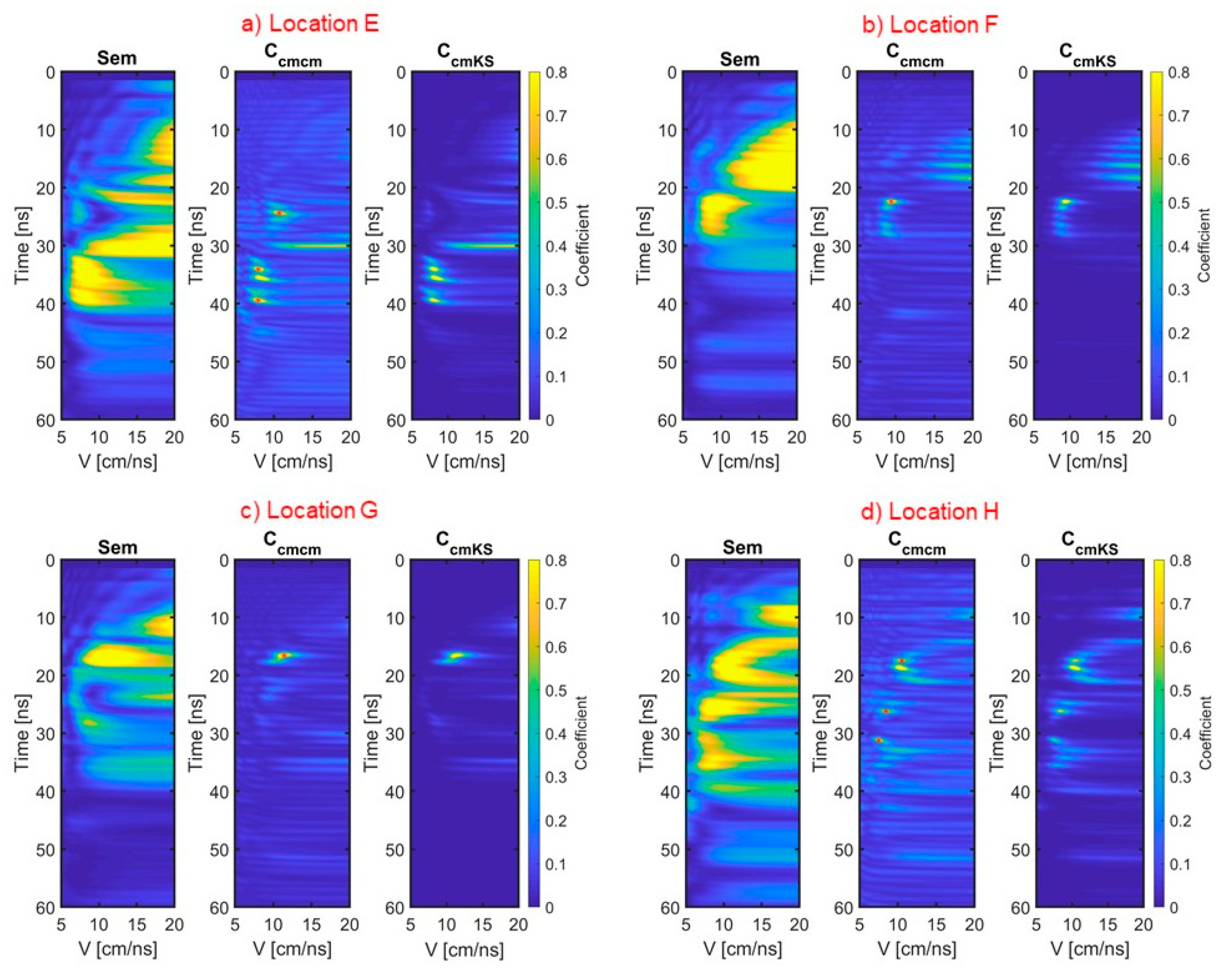
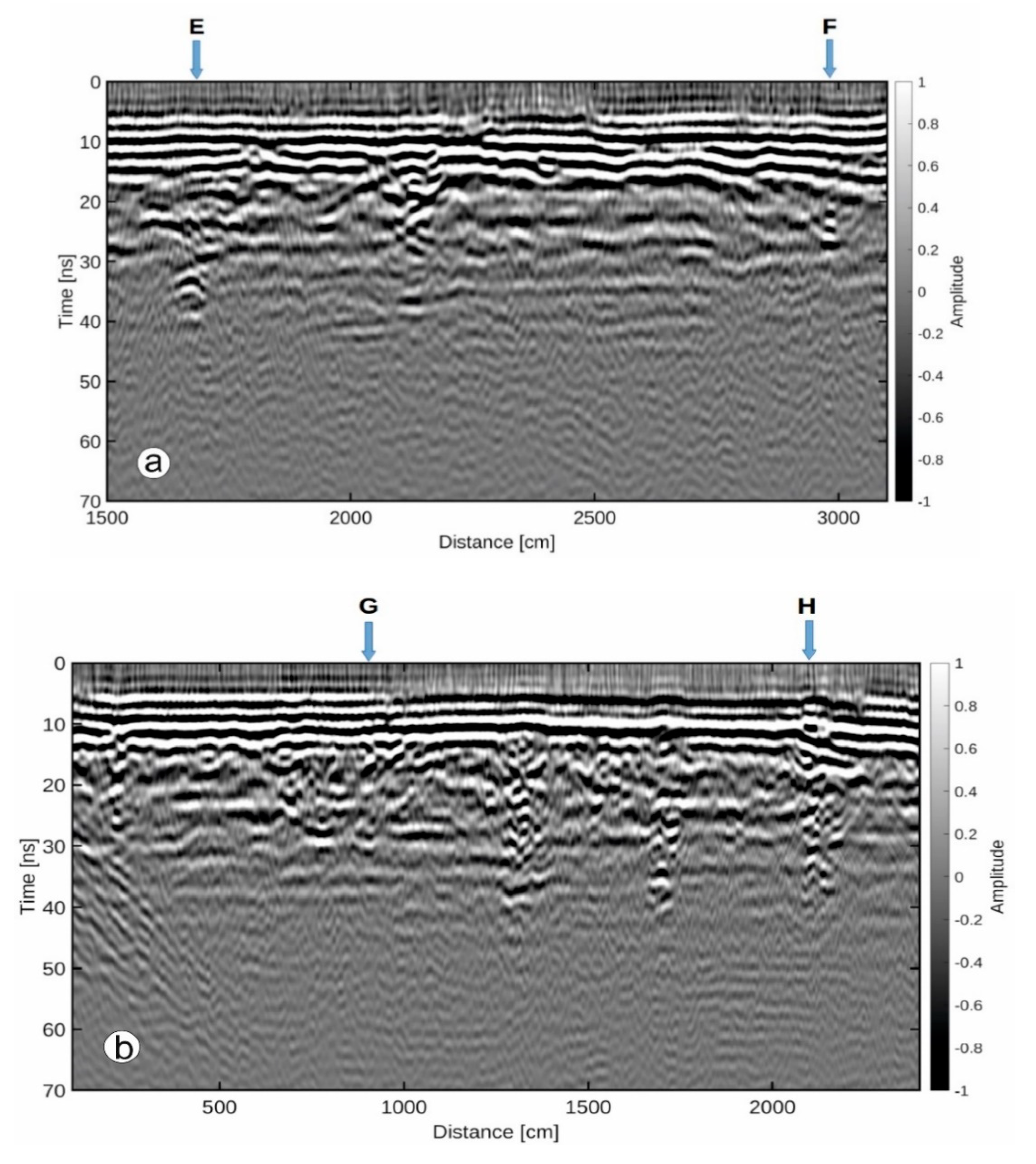
Coherency maps of GPR data can only be significant in correspondence with the diffracted energy that has a hyperbolic trajectory. Due to the time required to select the locations and to compute the coherency maps, we performed the velocity analysis only on some selected GPR profiles (L-lines) of the data set where the diffraction events are more evident. Figure 6a,b show a portion of the L74 and L92 lines with imposed the estimated trajectories after the velocity picking on the coherency panels. The different colors of the left and right arms of the hyperbolas allow for easier identification of the data used in the analysis. Indeed, after some attempts, we chose to employ a 64-sample time window around the right arm for the L74 line, and an identical window around the left arm for the L92 line. In Figure 7a–d we show the coherency panels used to pick the (t0,Vs) pairs and the values actually picked with red asterisks in positions E and F of L74, and G and H of L92. The velocity analysis in point E highlights the difficulties that may be found to match real diffraction patterns on GPR data. We selected the right arm (the use of the left one resulted in a too high velocity and an over-migrated section) and performed the analysis every 6 cm, eventually choosing the best velocity function on the basis of hyperbola fitting and migrated results. This made it possible to make a good compromise regarding the issue of possible uncertainties in velocity estimation due to the finite dimensions of the subsurface targets [8]. We made use of both the Ccmcm and the semblance functionals since the contribution of each of them was significant in the velocity analysis phase. Semblance was helpful for giving a rough indication of the regions in the (t0,Vs) map where the signal concentrates, while Ccmcm was useful for its higher resolution, which allows us to select more precise values and discard artefacts introduced by the semblance algorithm.
In Figure 7 we also show the CcmKS functional that is generally less noisy than the Ccmcm due to the Ccm weighting, but at least in case E was less effective. A possible explanation can be given by looking at the Semblance. The sample-by-sample weights introduced by the Ccm in the CcmKS, which are similar to the semblance, filter out the coherency observed around 22 ns at 10 cm/ns that was detected by the Ccmcm functional. Note that having more than a single coherency measure available (the ones displayed plus the Ccm which is very similar to the Semblance and therefore not shown) helps to better discriminate the (t0,Vs) pairs related to signal, leading to an improved velocity analysis. The parameters used for the real data case are indicated in Table 2. The velocity values obtained are used to build a velocity field and to migrate with a Kirchhoff algorithm the GPR profiles (L-lines) without imposing limits on the dip angle and on the available frequencies. This permits on the one hand to collapse all the hyperbola arms and on the other hand to preserve the maximum possible resolution allowed by the data. The migrated GPR profiles in Figure 6a,b are displayed in Figure 8a,b respectively, for an analysis of the results. As can be observed, along both profiles the diffracted energy is fairly collapsed in correspondence with the apex region (only point E appears slightly under-migrated), allowing us to better define the discontinuities in the subsurface.
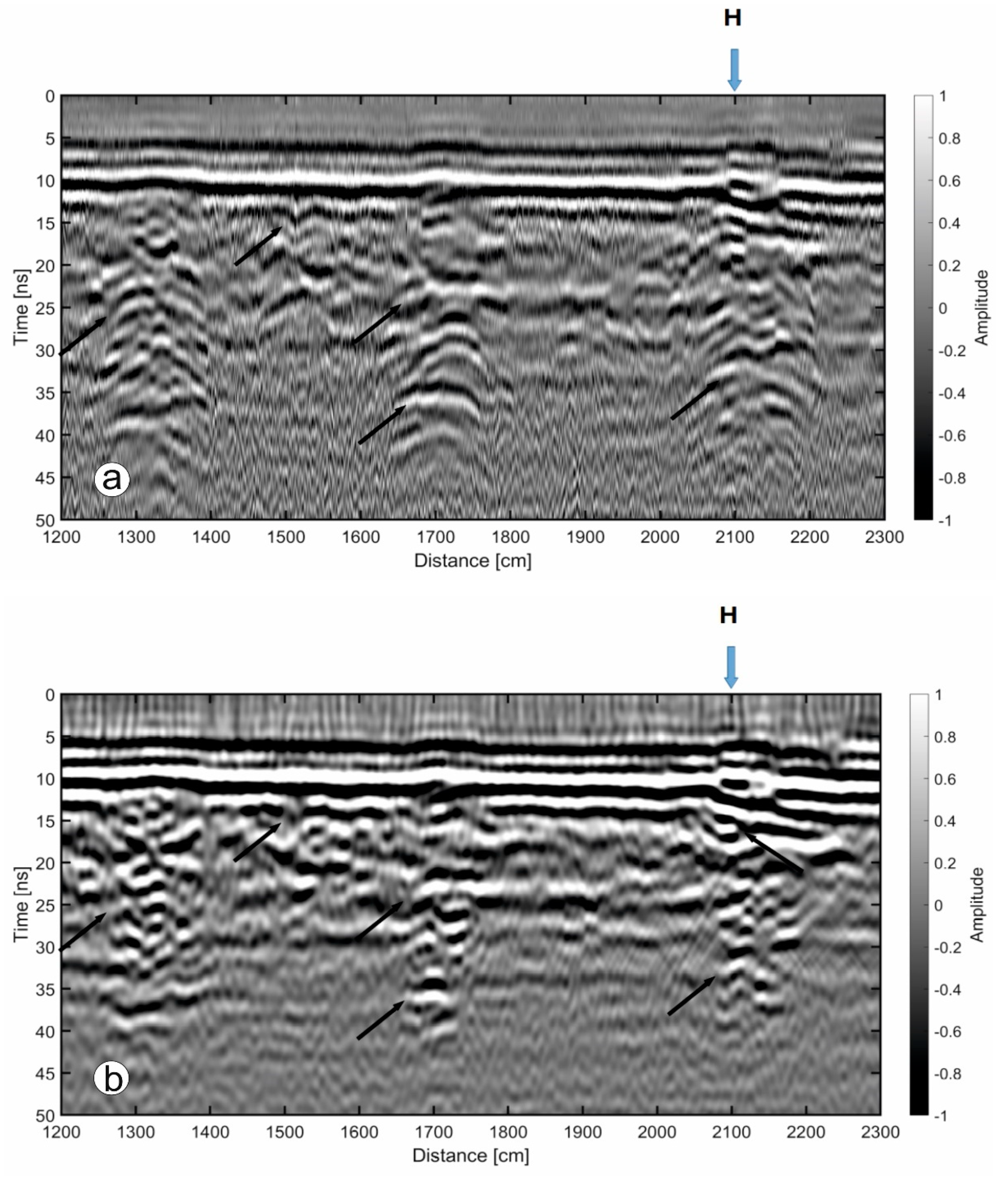
This is more evident in the close-up of Figure 9a,b pertaining to the L92 line before and after migration, where the arrows indicate some interesting locations. It can be observed that after migration, the dimension of the objects illuminated by the electromagnetic energy is laterally well-delimited, thus giving a more realistic description of the size and shape of the buried targets. Moreover, thanks to the multi-channel (multi-trace) filtering process operated by the migration operator, random noise is reduced after migration.
3.3. The Effect of Varying Velocity Field on Time-slices
The migrated GPR lines were used to build time-slices (amplitude maps) parallel to the surface and cut at different times. It is well known that this kind of representation is largely used to correlate spatially coherent reflected energy (i.e., reflections) with targets at different depths. Testing whether the high-coherency functionals increase the readability of reflective areas in a time-slice representation is thereby crucial. To do this, we gridded and sliced three GPR datasets: (i) unmigrated data, (ii) data migrated with a constant velocity (10 cm/ns), and (iii) data migrated according to the varying velocity field reconstructed via the high-coherency functionals described above. The value of 10 cm/ns, used for the constant velocity migration, comes from the average of the picked velocity values on the coherency maps relative to several GPR profiles. In building the time-slices, we took care to keep slicing and gridding parameter constant (slice thickness: 4 ns; the square amplitude of amplitude values; cell dimension: 0.05 m; search area: circular; search radius: 1 m), as well as the interpolation statistical method (i.e., inverse weighted distance).
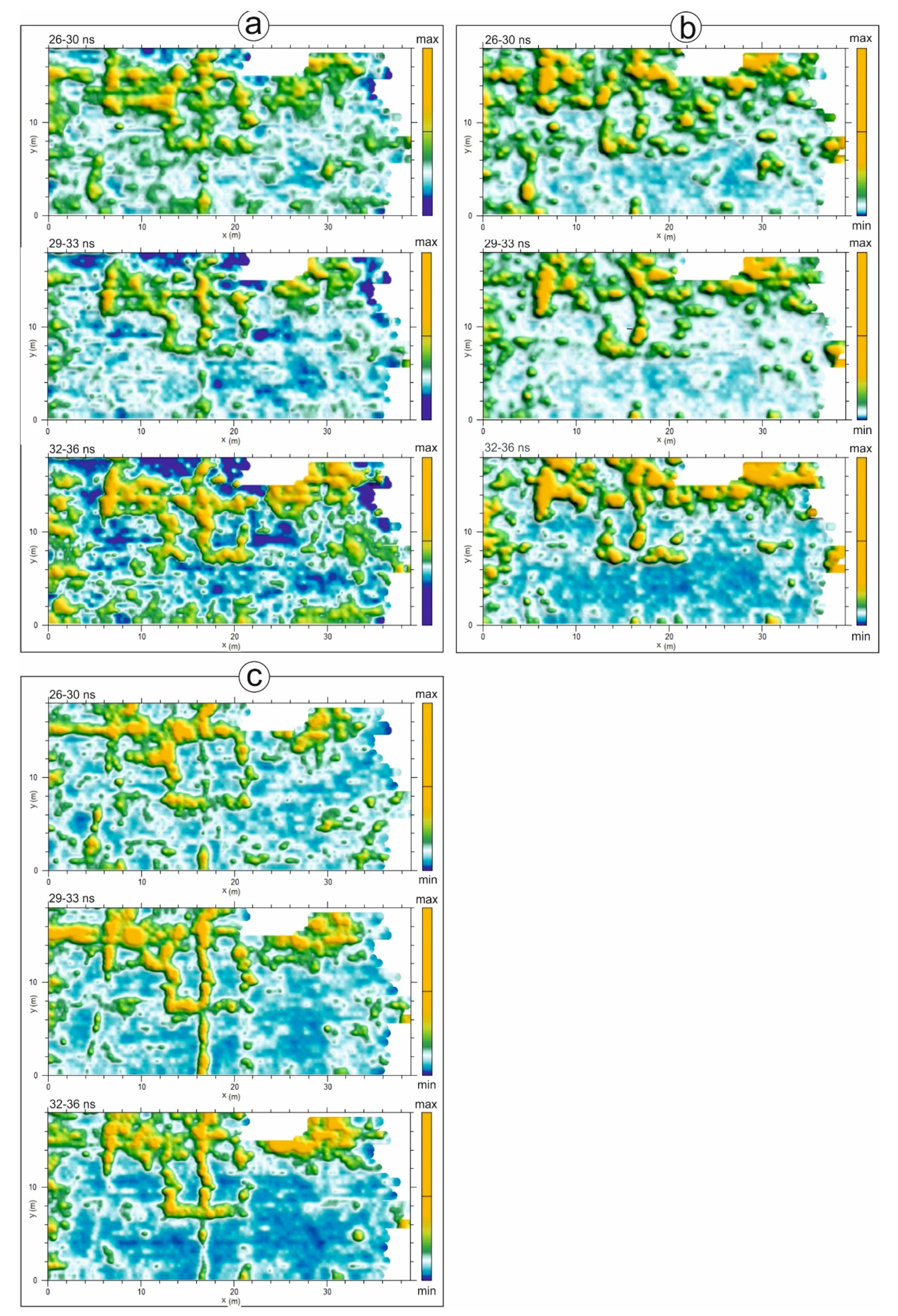
All these operations were performed with the GPRSlice software via Geophysical Archaeometry Laboratory [30]. For the sake of comparison, we illustrate only three time-slices in the temporal interval of 26–36 ns, centered at 28, 31, 34 ns and 4 ns thick (Figure 10). Instead of the same scale of reflection strength (amplitude), we used a relative normalization for each time-slice because this allows us to better imagine the subsurface targets and make the comparison more effective.
It is evident that the spatially-coherent reflective areas are clearer and of higher resolution in the time-slices built using the GPR lines migrated with a variable velocity field reconstructed via the high-resolution functionals (Figure 10). Moreover, the reflection intensity appears to have increased, and spot reflections, associated with local subsurface conditions (e.g., localized increases in density due to the presence of boulders/blocks concentrations or fragments of man-made remnants), are reduced. The time-slices built with GPR profiles migrated with a constant velocity (10 cm/ns) show content in amplitude higher than those built with un-migrated GPR profiles. However, in some sectors, it appears that the migration process has not favored the continuity of the reflections even if compared with those depicted in the un-migrated time-slices. This is an effect of the non-optimal velocity used in the migration that hampers the focusing of the reflected energy at the correct position.
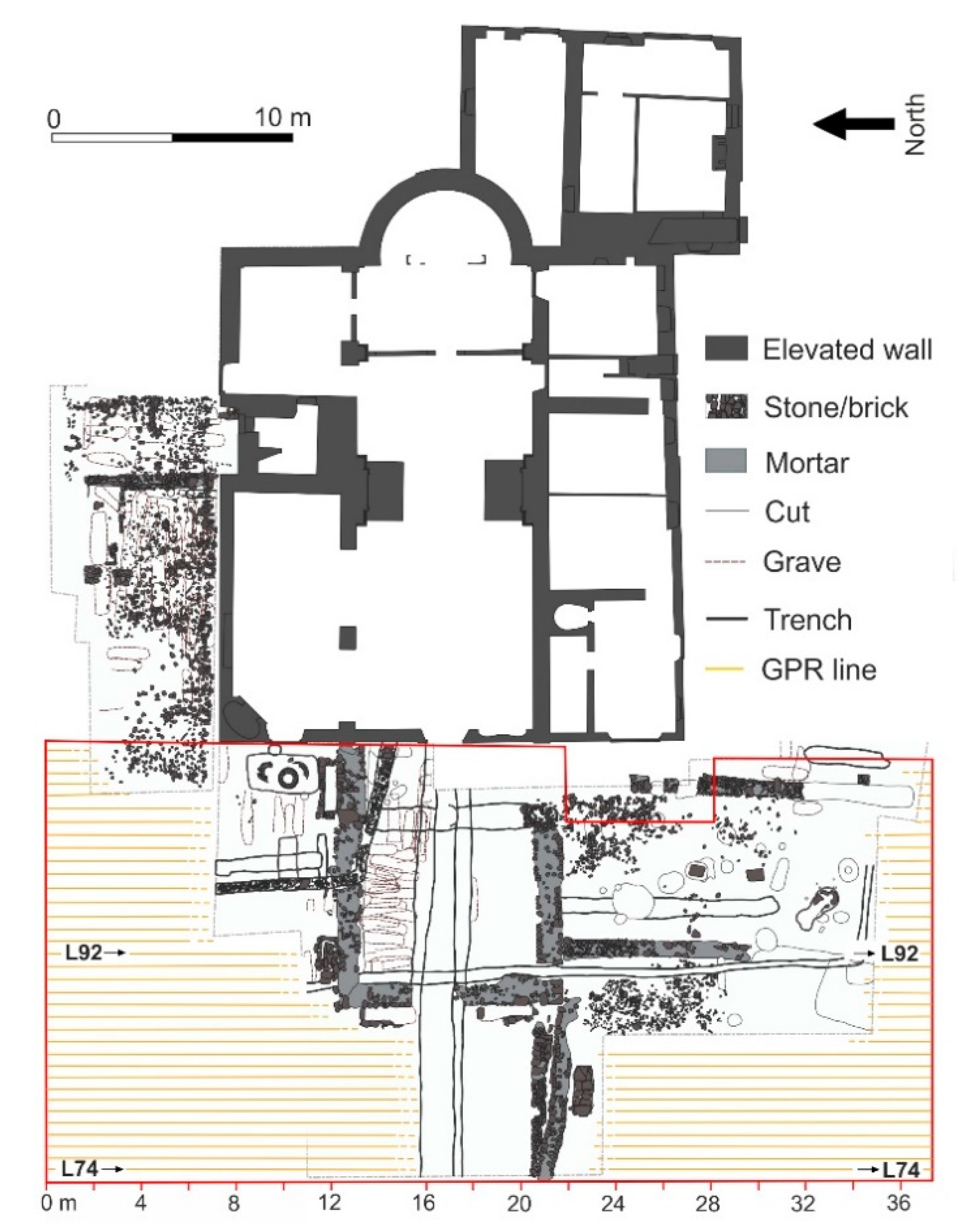
As can be seen from the comparison with the excavation results (Figure 1), the linear-shaped reflections are consistent with the archaeological findings unearthed in the investigation area. There is a clear correspondence both with masonry structures composed of stones/bricks and cuts consisting in channels for rainwater drainage. Relative to the channel EW crossing the central part of the time-slices (especially visible in the interval 29–33 ns), the backscattered energy from the filling material (coarse gravel and boulders) has returned in the GPR profiles hyperbolic diffractive figures, although with an irregular form [9]. Note that we selected only three time-slices ranging between 26–36 ns, and some of the archeological structures may be not evident in Figure 10 because they are shallower or deeper. Indeed, the evident NS-oriented wall developed between 22 and 30 m of horizontal distance is at about 5–10 ns.
The test of high-resolution functionals on such a kind of data was quite demanding. This is because the structure of the buried walls is composed laterally by interlocked decimetric boulders (interconnected boulders and open voids) and internally by boulders dispersed in an abundant mortar. In GPR profiles, the tops of these structures correspond to a planar reflection, while the boulders placed on the sides and corners of the wall to arms of hyperbolas (i.e., half hyperbolas) (see the black arrow pointing to 22 ns and 1700 cm of distance in Figure 9a). Moreover, the boulders in the mortar-dominant core generated small hyperbolic diffractions with interfering arms [9]. While the latter is difficult to model and manage even with a variable velocity field, the approach based on high-resolution functionals has clearly made possible a more than satisfactory focusing of the principal diffraction hyperbolas, and therefore a better definition of the wall structures in the time-slices.
4. Conclusions
The aim of this paper was to verify whether the use of high-resolution coherency functionals could improve the quality in terms of S/N ratio and interpretability of GPR data by introducing a variable velocity field in the migration process.
After carrying out tests on synthetic data to schematically simulate the problem, assessing the types of functionals most suitable for GPR data analysis, a varying velocity field relative to a real dataset was calculated. This dataset was acquired in an archaeological area for which the position of the targets was already available because these have been unearthed after the GPR survey.
The best functionals turned out to be the Ccmcm and the CcmKS, because they are able to compute coherency maps characterized by high resolution and strong noise rejection that make it possible to better define the time-velocity pairs of the observed diffracted events. In the velocity analysis, particular attention was paid to checking the fitting between the reconstructed diffraction hyperbola arms and those generated by buried structures, which do not consist of ideal scattering points but targets with a certain lateral extension as in most real cases. In the selected data, we did not include the top planar part of the event, limiting the application of the method to the hyperbola arms, reducing the possibility of wrong velocity estimation. We observed that with the precisely-picked 2D velocity field migration algorithms perform better than in the case of constant or 1D velocity field, with satisfactory collapsing of the diffracted events and moving of the reflected energy to the correct position.
The varying velocity field was applied to all the GPR profiles composing the survey and covering the entire archaeological area. The time-slices constructed are of a higher quality than those obtained from non-migrated or migrated GPR profiles at a constant velocity. The improvements are inherent to resolution, continuity, and energy amplitude of linear reflective areas.
On the basis of our experience, we can affirm that the use of high-resolution functionals allows us to obtain migrated GPR profiles with a high grade of hyperbola focusing. On these profiles, the targets of interest are better-imaged and the interpretation can be carried out more reliably. A varying velocity field, even sparsely sampled like the one we have built, can allow for more accurate positioning in time of the objects of interest with respect to the constant or 1D velocity model routinely used, or when no data migration is applied. This could be relatively important when studying an archaeological site or a geological setting, cases in which a slightly incorrect positioning of targets/layers is acceptable. However, accurate reconstruction of the target geometry and positioning becomes crucial when it comes to studying other topics, e.g., those related to civil engineering and micro-structural settings, where even modest velocity variations can lead to reconstruction errors which may be quite relevant.
The main drawbacks we experienced were the time required by the functional computation (approximately 5 min on an i7 laptop for each location) and the time required to choose the locations for performing the velocity analysis. Concerning this last issue, one suggestion could be to perform the velocity analysis on a whole line (or the more promising portions of a line) and then inspect the velocity volume (time, velocity, inline distance) to select the best coherency maps on which to perform the velocity analysis. This can be done at a very high computational cost but can save some manpower time. An alternative option could be exploiting automatic tools of hyperbola detection to generate a dataset of locations on which to perform the high-resolution velocity analysis. By applying the functionals only to this limited number of points, selected along the GPR profiles, allows us to limit computational costs.
Notwithstanding these drawbacks, we believe that in cases where an accurate and detailed image of the subsurface is desired, this methodology is worth the effort.
Author Contributions
Conceptualization, E.S. and A.R.; methodology, E.S. and A.T.; software, E.S., A.R. and A.T.; validation, E.S. and A.R.; formal analysis, E.S., A.R. and A.T.; investigation, E.S. and A.R.; resources, E.S., A.R. and A.T.; data curation, E.S. and A.R.; writing—original draft preparation, E.S. and A.R.; writing—review and editing, E.S., A.R. and A.T.; funding acquisition, A.R. All authors have read and agreed to the published version of the manuscript.
Funding
GPR data acquisition was funded by the CA.RI.LU grant: “New high resolution Georadar techniques for archeological contexts analysis” (Leader. A. Ribolini).
Acknowledgments
We thank the Landmark Graphics Corporation for the use of the ProMax software employed in the seismic data processing. We thank F. Coschino (University of Pisa) and A. Fornaciari (University of Pisa) for providing the archeological data. M. Bini (University of Pisa) and I. Isola (INGV, Pisa) cooperated in the GPR data acquisition. The comments of four anonymous reviewers were helpful to improve the manuscript.
Conflicts of Interest
The authors declare no conflict of interest.
References
- Davis, J.L.; Annan, A.P. Ground Penetrating Radar for high resolution mapping of soil and rock stratigraphy. Geophys. Prospect. 1989, 37, 531–551. [Google Scholar] [CrossRef]
- Annan, A.P. Electromagnetic principles of ground penetrating radar. In Ground Penetrating Radar: Theory and Applications; Jol, H.M., Ed.; Elsevier: Amsterdam, The Netherlands, 2009; pp. 3–40. [Google Scholar]
- Cassidy, N.J. Ground penetrating radar data processing, modelling and analysis. In Ground Penetrating Radar: Theory and Applications; Jol, H.M., Ed.; Elsevier: Amsterdam, The Netherlands, 2009; pp. 141–176. [Google Scholar]
- Persico, R. Introduction to Ground Penetrating Radar. Inverse Scattering and Data Processing; IEEE Press Wiley: Hoboken, NJ, USA, 2014; p. 400. [Google Scholar]
- Allroggen, N.; Tronicke, J.; Delock, M.; Böniger, U. Topographic migration of 2D and 3D ground-penetrating radar data considering variable velocities. Near Surf. Geophys. 2015, 13, 253–259. [Google Scholar] [CrossRef]
- Neidell, N.S.; Taner, M.T. Semblance and other coherency measures for multichannel data. Geophysics 1971, 36, 482–497. [Google Scholar] [CrossRef]
- Maas, C.; Schmalzl, J. Using pattern recognition to automatically localize reflection hyperbolas in data from ground penetrating radar. Comput. Geosci. 2013, 58, 116–125. [Google Scholar] [CrossRef]
- Laurence, M.; Persico, R.; Matera, L.; Lambot, S. Automated Detection of Reflection Hyperbolas in Complex GPR Images with no a priori knowledge on the medium. IEEE Trans. Geosci. Remote Sens. 2016, 54, 580–596. [Google Scholar]
- Ribolini, A.; Bini, M.; Isola, I.; Coschino, F.; Baroni, C.; Salvatore, M.C.; Zanchetta, G.; Fornaciari, A. GPR versus Geoarchaeological Findings in a Complex Archaeological Site (Badia Pozzeveri, Italy). Arch. Prosp. 2017, 24, 141–156. [Google Scholar] [CrossRef]
- Sguazzero, P.; Vesnaver, A. A comparative analysis of algorithms for seismic velocity estimation. In Deconvolution and Inversion; Bernabini, M., Rocca, F., Treitel, S., Worthington, M., Eds.; Blackwell: London, UK, 1987; pp. 267–286. [Google Scholar]
- Key, S.C.; Smithson, S.B. New approach to seismic-reflection event detection and velocity determination. Geophysics 1990, 55, 1057–1069. [Google Scholar] [CrossRef]
- Grion, S.; Mazzotti, A.; Spagnolini, U. Joint estimation of AVO and kinematics parameters. Geophys. Prospect. 1998, 46, 405–422. [Google Scholar] [CrossRef]
- Sacchi, M.D. A bootstrap procedure for high-resolution velocity analysis. Geophysics 1998, 63, 1716–1725. [Google Scholar] [CrossRef]
- Grandi, A.; Stucchi, E.; Mazzotti., A. Multicomponent velocity analysis by means of covariance measures and complex matched filters. In Proceedings of the 74th Annual International Meeting, Denver, CO, USA, 10–14 October 2004; Society of Exploration Geophysicists: Huston, TX, USA, 2004; pp. 2415–2418. [Google Scholar]
- Grandi, A.; Mazzotti, A.; Stucchi, E. Multicomponent velocity analysis with quaternions. Geophys. Prospect. 2007, 55, 761–777. [Google Scholar] [CrossRef]
- Abbad, B.; Ursin, B. High-resolution bootstrapped differential semblance. Geophysics 2012, 77, U39–U47. [Google Scholar] [CrossRef]
- Tognarelli, A.; Stucchi, E.; Ravasio, A.; Mazzotti, A. High-resolution coherency functionals for velocity analysis: An application for subbasalt seismic exploration. Geophysics 2013, 78, U53–U63. [Google Scholar] [CrossRef] [Green Version]
- Gong, X.; Wang, S.; Zhang, T. Velocity analysis using high-resolution semblance based on sparse hyperbolic Radon transform. J. Appl. Geophys. 2016, 134, 146–152. [Google Scholar] [CrossRef]
- Goodman, D.; Nishimura, Y.; Rogers, J.D. GPR timeslices in archaeological prospection. Archaeol. Prospect. 1995, 2, 85–89. [Google Scholar]
- Nuzzo, L.; Leucci, G.; Negri, S.; Carrozzo, M.T.; Quarta, T. Application of 3D visualization techniques in the analysis of GPR data for archaeology. Ann. Geophys. 2002, 45, 321–337. [Google Scholar]
- Leckebush, J. Ground-penetrating radar: A modern three-dimensional prospection method. Archaeol. Prospect. 2003, 10, 213–240. [Google Scholar] [CrossRef]
- Grasmueck, M.; Weger, R.; Horstmeyer, H. Three-dimensional ground-penetrating radar imaging of sedimentary structures, fractures, and archaeological features at submeter resolution. Geology 2004, 32, 933–936. [Google Scholar] [CrossRef]
- Soldovieri, F.; Orlando, L. Novel tomographic based approach and processing strategies for GPR measurements using multifrequency antennas. J. Cult. Herit. 2009, 10, 83–92. [Google Scholar] [CrossRef]
- Bini, M.; Fornaciari, A.; Ribolini, A.; Bianchi, A.; Sartini, S.; Coschino, F. Medieval phases of settlement at Benabbio castle, Apennine Mountains, Italy: Evidence from ground penetrating radar survey. J. Archaeol. Sci. 2010, 37, 3059–3067. [Google Scholar] [CrossRef]
- Tinelli, C.; Ribolini, A.; Bianucci, G.; Bini, M.; Landini, W. Ground penetrating radar and palaeontology: The detection of sirenian fossil bones under a sunflower field in Tuscany (Italy). Comptes Rendus Palevol 2012, 11, 445–454. [Google Scholar] [CrossRef]
- Fornaciari, A. Badia Pozzeveri. Dalla terra alla storia. LUK 2014, 20, 30–36. [Google Scholar]
- IDS GeoRadar. Available online: https://idsgeoradar.com/ (accessed on 12 May 2020).
- Spagnolini, U.; Maciotta, L.; Manni, A. Velocity analysis by truncated singular value decomposition. In Proceedings of the 63rd Annual International Meeting, Washington, DC, USA, 26–30 September 1993; Society of Exploration Geophysicists: Huston, TX, USA; pp. 677–680. [Google Scholar]
- Tognarelli, A.; Aleardi, M.; Mazzotti, A. Estimation of a high resolution P-wave velocity model of the seabed layers by means of global and a gradient-based FWI. In Proceedings of the Second Applied Shallow Marine Geophysics Conference, Barcelon, Spain, 4–8 September 2016; European Association of Geosciences and Engineering. [Google Scholar] [CrossRef]
- Geophysical Archaeometry Laboratory. Available online: https://www.gpr-survey.com/ (accessed on 12 May 2020).
- Goodman, D. Ground-penetrating radar simulation in engineering and archaeology. Geophysics 1994, 59, 224–232. [Google Scholar] [CrossRef]
- Yilmaz, O. Seismic Data Analysis: I—Processing, Inversion, and Interpretation of Seismic Data; Doherty, S.M., Ed.; Society of Exploration Geophysics: Tulsa, OK, USA, 2001; p. 2065. [Google Scholar]
Figure 1.
The archaeological site of Badia Pozzeveri. The plan of the elevated structures and of the unearthed archaeological findings is reported. The red box corresponds to the area surveyed with the GPR, and the yellow lines are the traces of the GPR profiles (the codes correspond to GPR profiles mentioned in the text). Although the GPR profiles entirely cover the area, they are interrupted to make the archaeological symbols more readable.

Figure 2.
The synthetic model adopted to simulate the appearance of diffraction hyperbolas in GPR profiles. Subsurface EM characteristics and simulation parameters are indicated. Surface locations of the objects are labelled A, B, C, and D. Tx: transmitter; Rx: receiver.
Figure 2.
The synthetic model adopted to simulate the appearance of diffraction hyperbolas in GPR profiles. Subsurface EM characteristics and simulation parameters are indicated. Surface locations of the objects are labelled A, B, C, and D. Tx: transmitter; Rx: receiver.

Figure 3.
The synthetic GPR section showing the events generated by the buried objects of the model in Figure 2. Two fitting hyperbolas with their left (magenta) and right (green) arms are also displayed. While in A the whole hyperbola matches quite well the observed diffraction, in D only the magenta arm shows a good fit. This is because only the left arm of the diffracted event is used in the velocity analysis. Including also the right arm would result in an incorrect velocity estimation due to the fact that the object in D, for its dimension, is not a point diffractor, and consequently the shape of the observed event is not a true hyperbola.

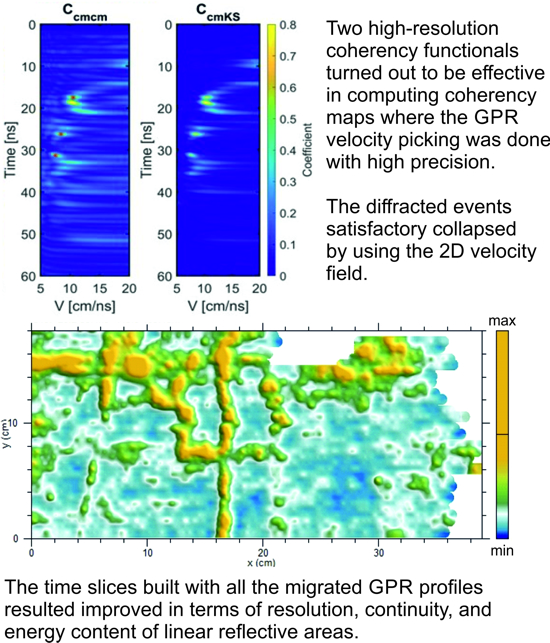
Figure 4.
(a) Map of the coherency measure in location A; (b) map of the coherency measure in location D. These maps are obtained by the following functionals: Semblance (Cs), Complex Matched Analysis (Ccm), Complex Matched Coherency Measure (Ccmcm), and CcmKS, the combination of Ccm and Ccmcm. The higher velocity resolution of the functionals that make use of the data covariance matrix is clearly observed. The red circles correspond to the picked (t0,Vs) pairs that characterize the hyperbolic trajectories plotted in Figure 3. Colour scale and gain are identical for all functionals.

Figure 5.
Migrated synthetic section using: (a) a constant velocity of 6.7 cm/ns; (b) 12.2 cm/ns; (c) a varying velocity field obtained by the velocity analysis in A, B, C and D. When the migration velocity is not correct, we obtain in (a) under-migrated data, A and B positions, and in (b) over-migrated data, C and D positions. Only in (c) are the events correctly migrated.

Figure 6.
(a) GPR section of the L74 Line containing the right arm (plotted in green) of the hyperbolae whose (t0,Vs) parameters are picked in the coherency panels of Figure 7a for the location E, and Figure 7b for the location F; we decided to fit the right arm of the misshapen hyperbola at 34 ns in E because it appears more regular. (b) GPR section of the L92 Line. In this case, the left arms (plotted in magenta) of the hyperbolae are displayed. Their (t0,Vs) parameters are picked on the coherency panels of Figure 7c for location G and Figure 7d for location H. The other magenta half-hyperbolae on the L92 Line correspond to additional positions where the velocity analysis has been carried out.


Figure 7.
Coherency maps of the Semblance (Cs), Complex Matched Coherency Measure (Ccmcm) and CcmKS functionals computed in locations E and F of Line 74 (a,b respectively), and G and H of Line 92 (c,d respectively). The red asterisks indicate the (t0,Vs) pairs picked and corresponding to the parameters of the hyperbolae shown in Figure 6a,b. The colour scale and gain are identical for all functionals.

Figure 8.
(a) The time-migrated section using the 2D picked velocity field of the L74 Line; (b) the time-migrated section using the 2D picked velocity field of the L92 line. The diffraction events shown satisfactory collapse at their apex, and the true geometry of the subsurface objects is better-imaged.

Figure 9.
(a) A close-up of the L92 section; (b) a close-up of the L92 migrated section. Migration has the effect of delineating with higher accuracy the geometry of the buried objects. The black arrows indicate some points in the section where the migration outcomes are particularly evident.
Figure 9.
(a) A close-up of the L92 section; (b) a close-up of the L92 migrated section. Migration has the effect of delineating with higher accuracy the geometry of the buried objects. The black arrows indicate some points in the section where the migration outcomes are particularly evident.

Figure 10.
Time-slices generated from (a) unmigrated data, (b) data migrated with a constant velocity field (10 cm/ns), and (c) data migrated according to the varying velocity field.
Figure 10.
Time-slices generated from (a) unmigrated data, (b) data migrated with a constant velocity field (10 cm/ns), and (c) data migrated according to the varying velocity field.


Table 1.
Parameters used in the velocity analysis on synthetic data by the coherency functionals.
| n | 64 | Number of Time Samples of the Velocity Analysis Window |
|---|---|---|
| win_ap | 101 | Aperture of the velocity analysis window (number of traces) |
| v | 4–20 | Velocity interval scanned by velocity analysis (cm/ns) |
| dv | 0.1 | Increment in the velocity scanned (cm/ns) |
| dt0 | 0.098 | Time increment in the functional computation (ns) |
| noise | 0.1 | Standard deviation of the added white noise to avoid functional singularity |
| wavelet | 600 MHz | Maximum of the Ricker wavelet frequency spectrum |
Table 2.
Parameters used in the velocity analysis on real data by the different functionals.
| n | 64 | Number of Time Samples of the Velocity Analysis Window |
|---|---|---|
| win_ap | 81 | Aperture of the velocity analysis window (number of traces) |
| v | 4–20 | Velocity interval scanned by velocity analysis (cm/ns) |
| dv | 0.1 | Increment in the velocity scanned (cm/ns) |
| dt0 | 0.098 | Time increment in the functional computation (ns) |
| wavelet | 400 MHz | Maximum of the Ricker wavelet frequency spectrum |
© 2020 by the authors. Licensee MDPI, Basel, Switzerland. This article is an open access article distributed under the terms and conditions of the Creative Commons Attribution (CC BY) license (http://creativecommons.org/licenses/by/4.0/).
Share and Cite
MDPI and ACS Style
Stucchi, E.; Ribolini, A.; Tognarelli, A. High-Resolution Coherency Functionals for Improving the Velocity Analysis of Ground-Penetrating Radar Data. Remote Sens. 2020, 12, 2146. https://doi.org/10.3390/rs12132146
AMA Style
Stucchi E, Ribolini A, Tognarelli A. High-Resolution Coherency Functionals for Improving the Velocity Analysis of Ground-Penetrating Radar Data. Remote Sensing. 2020; 12(13):2146. https://doi.org/10.3390/rs12132146
Chicago/Turabian StyleStucchi, Eusebio, Adriano Ribolini, and Andrea Tognarelli. 2020. "High-Resolution Coherency Functionals for Improving the Velocity Analysis of Ground-Penetrating Radar Data" Remote Sensing 12, no. 13: 2146. https://doi.org/10.3390/rs12132146
Note that from the first issue of 2016, this journal uses article numbers instead of page numbers. See further details here.