Spatio-Temporal Variability of Chlorophyll-A and Environmental Variables in the Panama Bight

Abstract

The analysis of synoptic satellite data of total chlorophyll-a (Chl-a) and the environmental drivers that influence nutrient and light availability for phytoplankton growth allows us to understand the spatio-temporal variability of phytoplankton biomass. In the Panama Bight Tropical region (PB; 1–9°N, 79–84°W), the spatial distribution of Chl-a is mostly related to the seasonal wind patterns and the intensity of localized upwelling centers. However, the association between the Chl-a and different physical variables and nutrient availability is still not fully assessed. In this study, we evaluate the relationship between the Chl-a and multiple physical (wind, Ekman pumping, geostrophic circulation, mixed layer depth, sea level anomalies, river discharges, sea surface temperature, and photosynthetically available radiation) and chemical (nutrients) drivers in order to explain the spatio-temporal Chl-a variability in the PB. We used satellite data of Chl-a and physical variables, and a re-analysis of a biogeochemical product for nutrients (2002–2016). Our results show that at the regional scale, the Chl-a varies seasonally in response to the wind forcing and sea surface temperature. However, in the coastal areas (mainly Gulf of Panama and off central-southern Colombia), the maximum non-seasonal Chl-a values are found in association with the availability of nutrients by river discharges, localized upwelling centers and the geostrophic circulation field. From this study, we infer that the interplay among these physical-chemical drivers is crucial for supporting the phytoplankton growth and the high biodiversity of the PB region.

1. Introduction

Phytoplankton are the major primary producers in the ocean, being the base of the marine food web through the photosynthetic fixation of carbon and an essential component of the marine biogeochemical cycles [1,2]. Phytoplankton growth is mainly influenced by light and nutrient availability in the upper ocean. These conditions are controlled by several environmental variables and physical processes influencing the composition and abundance of phytoplankton, which determines the functioning of marine ecosystems [3,4,5]. Several studies have considered the link between the physical processes influencing changes in the phenological cycles of phytoplankton (based on chlorophyll-a (Chl-a) concentration as a proxy of phytoplankton biomass) and community structure [6,7,8,9,10].

In low-latitude regions (tropics), a long period of phytoplankton growth (~15–20 weeks) and a low amplitude in the annual cycle of Chl-a (<0.5 mg m⁻³) are mostly controlled by the input of nutrients to the surface layer [5]. By contrast, short growing periods (<10 weeks) with higher Chl-a values (>7 mg m⁻³) have been observed at high latitudes, as a result of light availability [5]. In the tropics, the Eastern Tropical Pacific (ETP) occupies 9% of the global ocean area and contributes 10% of the world’s oceanic productivity [11]. However, open ocean areas in the ETP are mainly oligotrophic with low Chl-a concentration (~0.3 mg m⁻³) and only few localized regions present high Chl-a values (e.g., ~1.05 mg m⁻³ in the Gulf of Papagayo, ~0.98 mg m⁻³ in Tehuantepec and ~1.06 mg m⁻³ in Panama). In general, these high Chl-a values have been found during the boreal winter (December to April, dry season in the ETP) in association with intense wind jets as a result of the intensification of the trade winds crossing Central America [12,13]. These jets can produce an intense wind stress curl, promoting sea surface divergence and upwelling, favoring the input of nutrients towards the upper layer and phytoplankton growth [11,14].

At the interannual scale, these oceanographic conditions are modified by the influence of El Niño Southern Oscillation (ENSO), a driver of large-scale natural climate variability, consisting of a warm (El Niño) and a cold (La Niña) phase [15]. During the ENSO events, anomalous variations in the strength of the trade winds and sea surface temperature in the tropics occur [16,17], including variations in ocean biogeochemical processes [18,19]. Regional decreases in Chl-a and primary production during El Niño events are associated with the perturbation in the wind forcing, causing variations in the advective fluxes of nutrients towards the upper layer [18,19,20,21]. In addition, the long and persistent positive sea surface temperature anomalies enhance the vertical stratification and deepen the thermocline in the tropical Pacific [22,23]. This, along with a deepening of the nutricline, decreases the availability of nutrients and dilutes the phytoplankton cells in the upper layer, restricting sunlight for photosynthesis and phytoplankton growth, and this is reflected in their biomass decrease [19,20,24]. By contrast, during La Niña events, high Chl-a and high phytoplankton biomass are observed due to the steepening of the basin gradient of the thermocline and nutricline across the tropical Pacific. This promotes the upwelling of water with high nitrate and iron concentrations into the euphotic layer in the eastern Pacific and, therefore, higher phytoplankton growth [22,24,25]. The ENSO effects are also reported for coral reefs in the tropics, which exhibit patterns of recovery and resilience in the ETP, except under extreme temperature events [26]. ENSO effects are also found in the high food web levels, such as changes in the structure and composition of euphausiid assemblage in the Colombian Pacific [27].

In the ETP, the Panama Bight (PB) ecoregion is located between the Isthmus of Panama and Punta Santa Elena (Ecuador), including the oceanic region off the coasts of Panama and Colombia [28,29]. In this ecoregion, the oceanic regional signal of total Chl-a displays a strong seasonal variability mostly related to the meridional migration of the Intertropical Convergence Zone (ITCZ) [11,30]. During the dry season (December to April), when the ITCZ is located in its southern position, the maximum oceanic Chl-a values are observed [30,31]. The increment in phytoplankton biomass during this period has been related to the influence of the Panama jet promoting localized upwelling centers and the geostrophic circulation characterized by a cyclonic gyre, which brings deep water towards the upper layer [11,32]. By contrast, the minimum Chl-a values are reported in the PB during the rainy season (May to November), when the ITCZ is located in its northern position [11,30]. During this period, the Panama jet is replaced by the Choco jet and the sea surface circulation is dominated by an anticyclonic gyre generating downwelling [33,34,35,36]. Despite all this knowledge, most of the studies related to Chl-a in the PB are fragmented in time and space, and to the best of our knowledge, no previous studies have included multiple physical and chemical drivers to explain the phytoplankton dynamics.

Besides this seasonal-regional Chl-a variability, differences in the annual cycle of Chl-a are also found between the coastal areas off Colombia and Panama. In the Colombian coast, the Chl-a concentration is elevated throughout the year, coinciding with localized upwelling centers [30]. In Panama, on the other hand, the Chl-a variability is found to have a seasonal signal with maximum (minimum) values during the dry (rainy) season when the mixed layer and the thermocline become shallower (deeper), promoting (suppressing) the input of nutrients towards the sea surface [37]. In addition, the PB is one of the rainiest regions of the world, with precipitation of ~8000 to 13,000 mm in the Colombian Pacific (CP) and ~2924 mm in Panama [38,39]. High rainfall rates influence the amount and timing of river discharges providing nutrients, such as iron and silicate, from the river basins to the continental shelf [11,40,41]. Nevertheless, the partial contribution of nutrient input to the coastal zones of the PB, due to localized upwelling centers and/or rivers discharges, has not been explored yet; nor has the influence of multiple other environmental drivers on the Chl-a signal.

In this study, the spatial heterogeneity of the Chl-a annual signal in the PB was assessed at the regional and local (subdomains) scales, considering (1) bathymetry features, (2) seasonal and non-seasonal oceanographic/atmospheric processes, (3) river discharges, and (4) nutrient content. For this purpose, we considered the seasonal climatology of Chl-a for the period 2002–2016 and explored the associations among different environmental drivers and Chl-a through a multivariate statistical analysis. The key factors contributing to the modulation of the phytoplankton biomass in the PB are discussed.

2. Materials and Methods

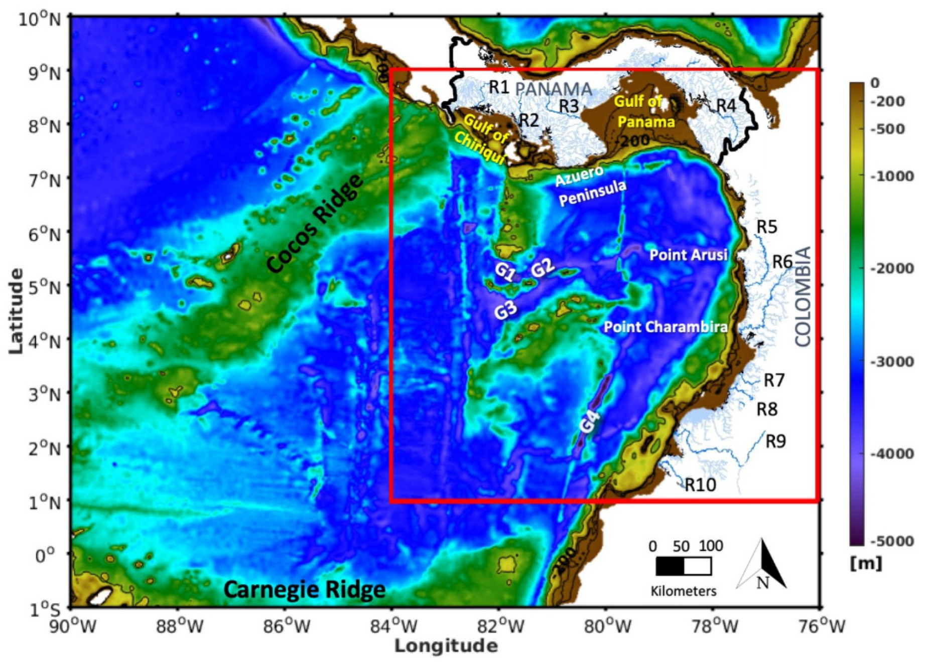
2.1. General Features of the Study Area

The PB (1–9°N, 76–84°W) includes the oceanic areas off Panama (Gulf of Chiriqui and Gulf of Panama) and Colombia (CP Ocean; 0 1). The ocean basin limits have the Cocos dorsal on their west side and the Carnegie dorsal on their southern edge, both with a maximum depth of ~2500 m. Inside the PB, there are two other dorsals—Coiba and Malpelo—which rise to a depth between ~500 and 1000 m [42]. These submarine mountains, trenches and depressions (the Panama fracture zone; the Colombian trench; and depressions of Yaquina, Omagua, Guanibos and Yurupar) determine the exchange and movement of water masses in the PB. Additionally, the continental shelf presents different dimensions along the PB coast. The Gulf of Panama shows the widest continental shelf (~125 km from the coast), followed by the Gulf of Chiriqui (~75 km) and Colombia (~50 km). The northern region off Colombia exhibits the narrowest shelf (~10 km; Figure 1). The circulation is influenced by elevated rates of rainfall, high freshwater discharge from several rivers, seasonal variability in the wind stress, and variations in the geostrophic circulation field [32,43].

2.2. Surface Satellite Chlorophyll-a

Daily images of Chl-a were downloaded from the Ocean Colour Climate Change Initiative (OC-CCI; version 3.1) for the period 2002–2016. The OC–CCI is a merged Level 3 product with a spatial resolution of 4 km, available at http://www.oceancolour.org/. The OC-CCI Chl-a dataset is retrieved by the combining of the observational data from the MERIS (MEdium spectral Resolution Imaging Spectrometer) sensor of the European Space Agency, the SeaWiFS (Sea-viewing Wide-Field-of-view Sensor) and MODIS-Aqua (Moderate-resolution Imaging Spectroradiometer-Aqua) sensors from the National Aeronautics and Space Administration (NASA-USA), and the VIIRS (Visible and Infrared Imaging Radiometer Suite) from the National Oceanic and Atmospheric Administration (NOAA-USA). The remote sensing reflectance data derived from the sensors were merged by band-shifting and bias-correcting the MERIS, MODIS and VIIRS data to match with the SeaWiFS data. Then, a selected in-water algorithm, based on water type, was applied to this merged dataset in order to generate the daily images of Chl-a concentration, including per-pixel uncertainty estimates. Due to the complexity of the study region, version 3.1 of the OC-CCI product was selected as it improves the performance of the ocean color data in coastal Case-2 waters compared to earlier versions that mostly focus on open ocean waters [44]. In addition, monthly composites of normalized fluorescence line height (nFLH) for phytoplankton fluorescence activity, at processing level 3 and spatial resolution of 4 km, were downloaded from the MODIS-Aqua mission (http://oceancolor.gsfc.nasa.gov/), for the period 2002–2016 (Appendix A).

2.3. Physical Environmental Drivers

Daily surface wind data, with a spatial resolution of 0.25° (~25 km), were acquired from the product V2 CCMP L3.0 (Cross-Calibrated, Multi-Platform Ocean Surface Wind Velocity; http://www.remss.com/measurements/ccmp/). This product integrates measurements from the Version-7 RSS radiometer wind speeds, QuikSCAT and ASCAT scatterometer wind vectors, moored buoy wind data and ERA-Interim wind fields.

The wind stress (τ) was computed from the monthly wind fields as follows:

$$\mathsf{\tau }={\mathsf{\rho }}_{\mathrm{a}}{\mathrm{C}}_{\mathrm{d}}\left|{\mathrm{V}}_{10}\right|{\mathrm{V}}_{10}$$

(1)

where C_d = 0.0015 is the drag coefficient, ρ_a = 1.2 kg m⁻³ is the mean air density, and V₁₀ is the wind speed at 10 m above the sea surface. The wind stress curl was estimated using the zonal and meridional components of the wind stress:

$${\left(\nabla \times \mathsf{\tau }\right)}_{\mathrm{z}}=\frac{\partial {\mathsf{\tau }}_{\mathrm{y}}}{\partial \mathrm{x}}-\frac{\partial {\mathsf{\tau }}_{\mathrm{x}}}{\partial \mathrm{y}}$$

(2)

This procedure was performed for each grid point by applying the centered finite difference algorithm, and the Ekman pumping velocity was estimated according to [36,45] as follows:

$$W_E=\frac{{\left(\nabla \times \mathsf{\tau }\right)}_{\mathrm{z}}}{ƒ{\mathsf{\rho }}_{\mathrm{w}}}+\frac{\mathsf{\beta }{\mathsf{\tau }}_{\mathrm{x}}}{{ƒ}^2{\mathsf{\rho }}_{\mathrm{w}}}$$

(3)

where τ_x is the zonal wind stress component, β = (2Ωcosφ/R) is the latitudinal variability of the Coriolis parameter (f = 2Ωsenφ), R = 6,371,000 m is the radius of the earth and ρ_w = 1025 kg m⁻³ is the mean water density. Positive (negative) values of Ekman pumping indicate upward (downward) water motion.

Daily surface geostrophic velocity fields and sea level anomaly (SLA) data were obtained from the Copernicus Marine and Environment Monitoring Service (CMEMS; http://marine.copernicus.eu/) with a spatial resolution of 0.25° (~25 km). The mixed layer depth (MLD) was estimated following the density criteria in the algorithm of [46], which is available from the NOAA Monthly Isopycnal and Mixed-layer Ocean Climatology (MIMOC) [47,48] with a spatial resolution of 0.5° (~50 km). The MIMOC product is based mostly on Argo data, supplemented by shipboard and Ice-Tethered Profiler conductivity-temperature-depth (CTD) data, and data from the World Ocean Database (http://www.pmel.noaa.gov/mimoc/).

Daily sea surface temperature (SST) and photosynthetically available radiation (PAR) data were obtained from the Multi-scale Ultra-high Resolution Sea Surface Temperature product (MUR-SST; https://podaac.jpl.nasa.gov/Multi-scale_Ultra-high_Resolution_MUR-SST, with a 1 km spatial resolution) and from the MODIS-Aqua mission (http://oceancolor.gsfc.nasa.gov/, with a 9 km spatial resolution), respectively. Daily images were averaged in monthly composites in order to aggregate all datasets into monthly intervals.

2.4. River Discharges

Monthly discharge data from the main rivers off the Panama and Colombia coasts were obtained from ETESA (Empresa Transmisión Eléctrica, Panama) and IDEAM (Instituto de Hidrología, Meteorología y Estudios Ambientales, Colombia) [49,50]. In addition, monthly composites of remote sensing reflectance at 645 nm (Rrs645), as a proxy of turbid plumes from river discharges, were obtained from the MODIS-Aqua mission (http://oceancolor.gsfc.nasa.gov/) for the period 2002–2016, at processing level 3 and a 4 km spatial resolution (Appendix A).

2.5. Nutrient Content

Monthly data of surface (~0.5 m depth) nutrient (silicate, nitrate and phosphate) and iron concentrations for the period 2002–2016 were obtained from the Ocean Biogeochemistry Non Assimilative Hindcast (Pisces) product from the Copernicus Marine and Environment Monitoring Service (CMEMS; http://marine.copernicus.eu/) with a spatial resolution of 0.25° (~25 km).

2.6. Data Processing and Statistical Analysis

The mean annual cycles of Chl-a, nutrient content and physical variables in the study region were characterized through monthly mean climatology. In the case of total Chl-a, a standard Empirical Orthogonal Function (EOF) analysis was performed in order to evaluate the principal modes of the Chl-a variability in the PB. For this, the spatial and temporal patterns of Chl-a were determined using the singular value decomposition (SVD) technique, which decomposes the space-time dataset into a linear combination of orthogonal standing oscillations (EOF modes) [51]. The SVD method estimates the temporal amplitudes of the spatial eigenvectors and their associated eigenvalues, allowing us to quantify the total variance of the Chl-a concentration in both orthogonal and independent modes. These are the modes or structures containing the highest percentage of the Chl-a variability that enable the assessment of (i) the most contrasting areas of the spatial Chl-a variability, and (ii) the main contrasting months in terms of the temporal annual Chl-a variability in the PB. This approach has been successfully used to interpret the space-time features of Chl-a data [52,53].

To assess the regional association between the Chl-a and its predicting physical variables for the most contrasting months, a multivariate analysis was performed using the Primer-E7 Software through a distance-based linear model (DISTLM) [54]. This analysis consists of a permutational test for the multivariate null hypothesis of no relationship between the Chl-a and the physical variables as predictors, on the basis of a resemblance measure (dissimilarity matrix D), using permutations of the samples to obtain a p-value. Therefore, it is possible to determine the variation in the data (described by D) that is explained by each physical variable. To find the best explanatory model from all the possible combinations of the predictor variables, this analysis followed a step-wise procedure selection and Akaike’s information criterion (AIC) [55]. The smallest achieved value of AIC indicates the best model, i.e., the best combination of the environmental predictor variables that explains the largest amount of the variation in the response variable (Chl-a). Additionally, further marginal tests explain the percentage variance of the Chl-a when each environmental variable is considered individually through a Pseudo-F value, which is a direct multivariate analogue of the Fisher’s F ratio used for standard regressions. The higher the Pseudo-F value, the higher the probability of the null hypothesis being false, i.e., a higher Pseudo-F value indicates a high probability of a relationship between the Chl-a and the physical variable as a predictor.

Then, from the resemblance dissimilarity matrix, a non-metric multidimensional scaling ordination (nMDS) was performed to assess the spatial differences of the Chl-a values across the PB by dividing the region into several subdomains (coastal and oceanic), which were used as the factors [56]. A multidimensional scaling analysis is an ordination method used to reduce the dimensionality of the data, allowing the detection of the most prominent observable patterns and structures. In particular, the non-metric multidimensional scaling focuses on preserving the rank order of the inter-point dissimilarities allowed within the constraints of a small number of dimensions (two or three). The procedure is based on the minimization of a monotonic function of the dissimilarities that is called “stress”. In consequence, the suitability of the resulting plot is determined by how well the inter-point distances in the reduced dimension correspond to the rank orders of the underlying dissimilarities [57,58], allowing us to visualize how different the subdomains are in terms of their Chl-a concentration values. Finally, linear Pearson correlations between Chl-a and the physical and chemical variables in each subdomain were calculated, in order to analyze the prominent factors promoting the low or high Chl-a values. For this, all the variables were re-gridded to the lowest spatial resolution (~25 km), excluding the MLD fields from the analysis due to their coarser resolution (~50 km).

3. Results

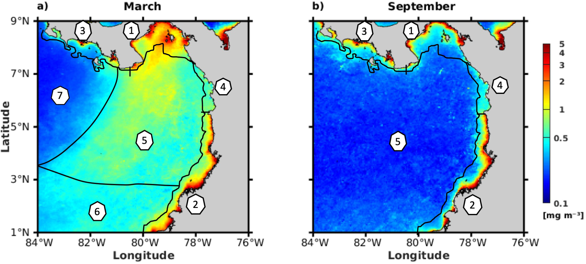
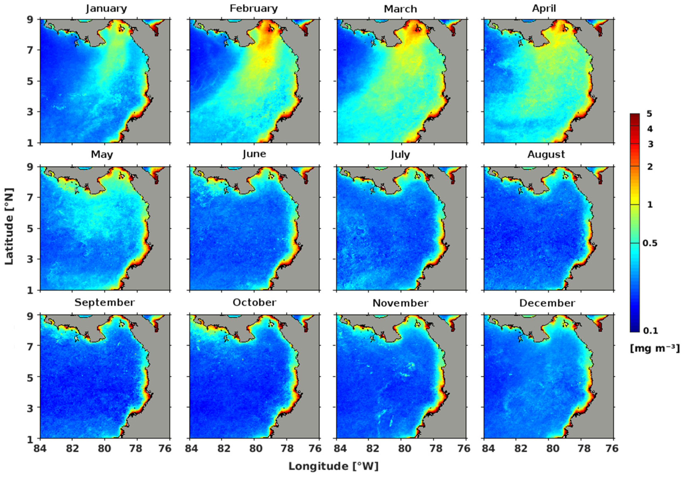
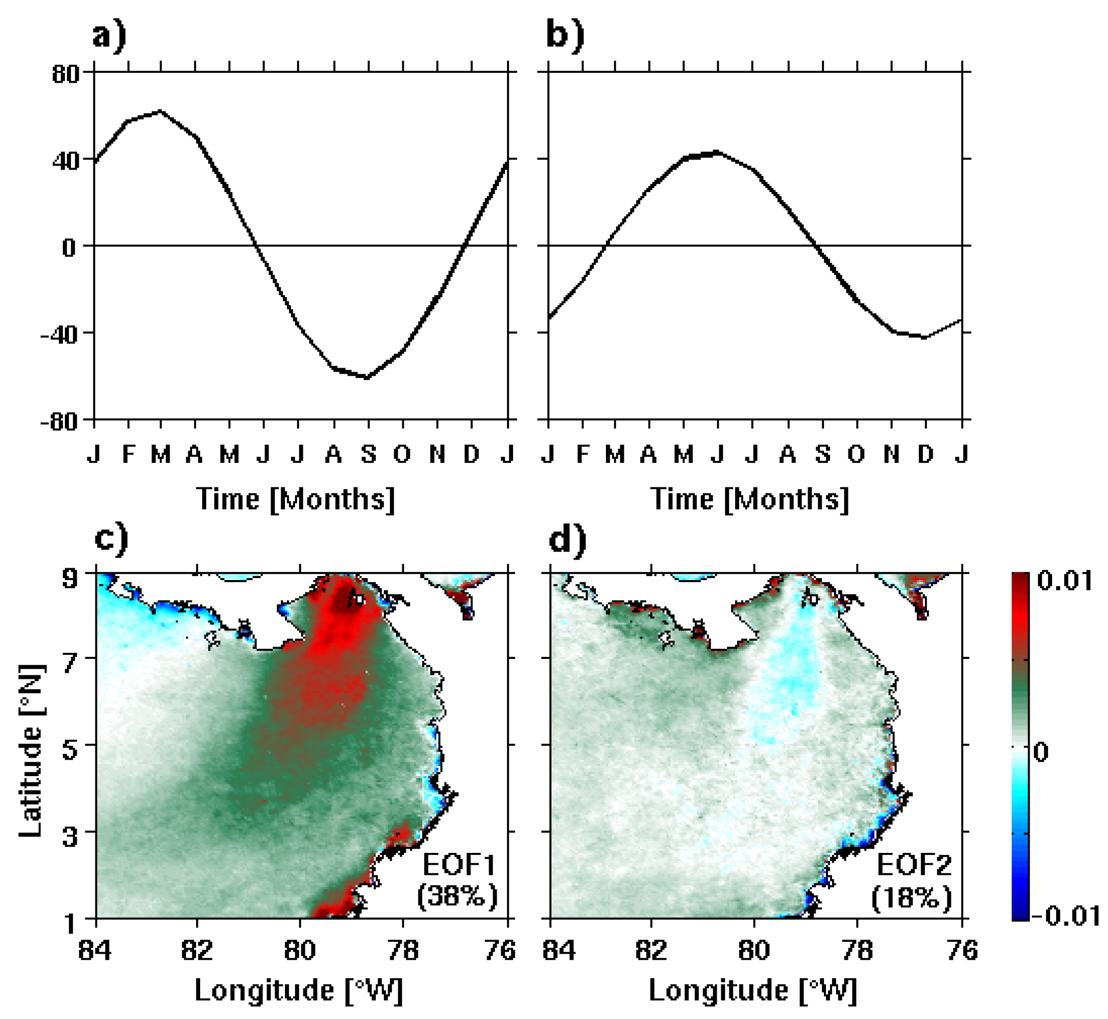
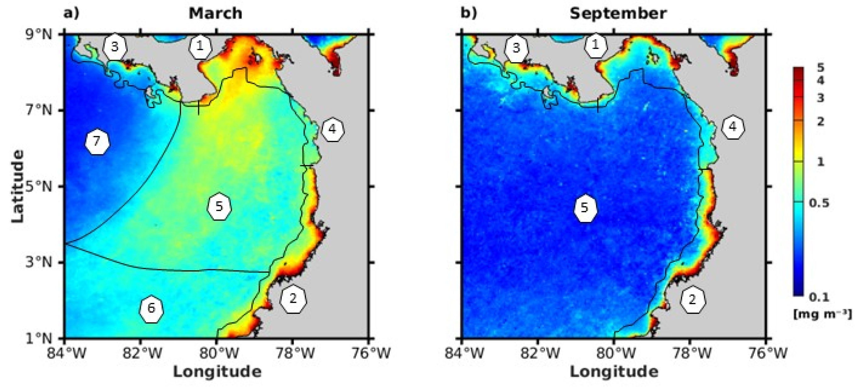
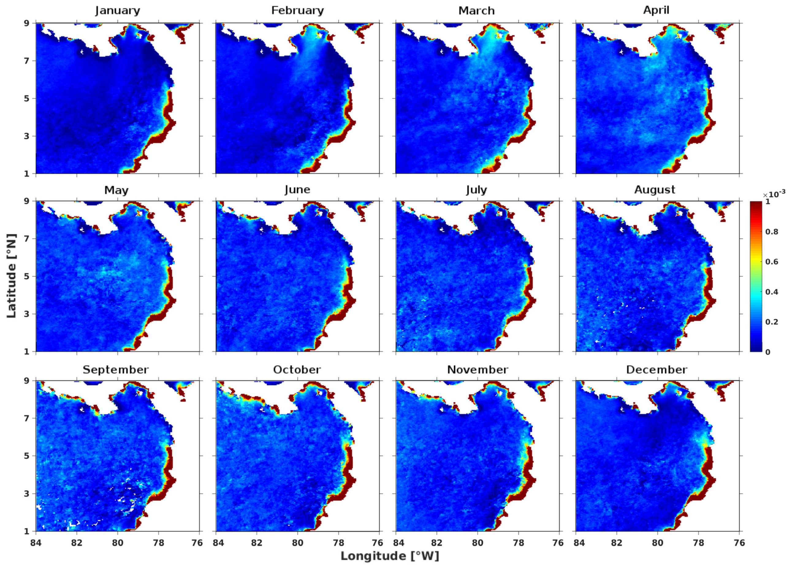
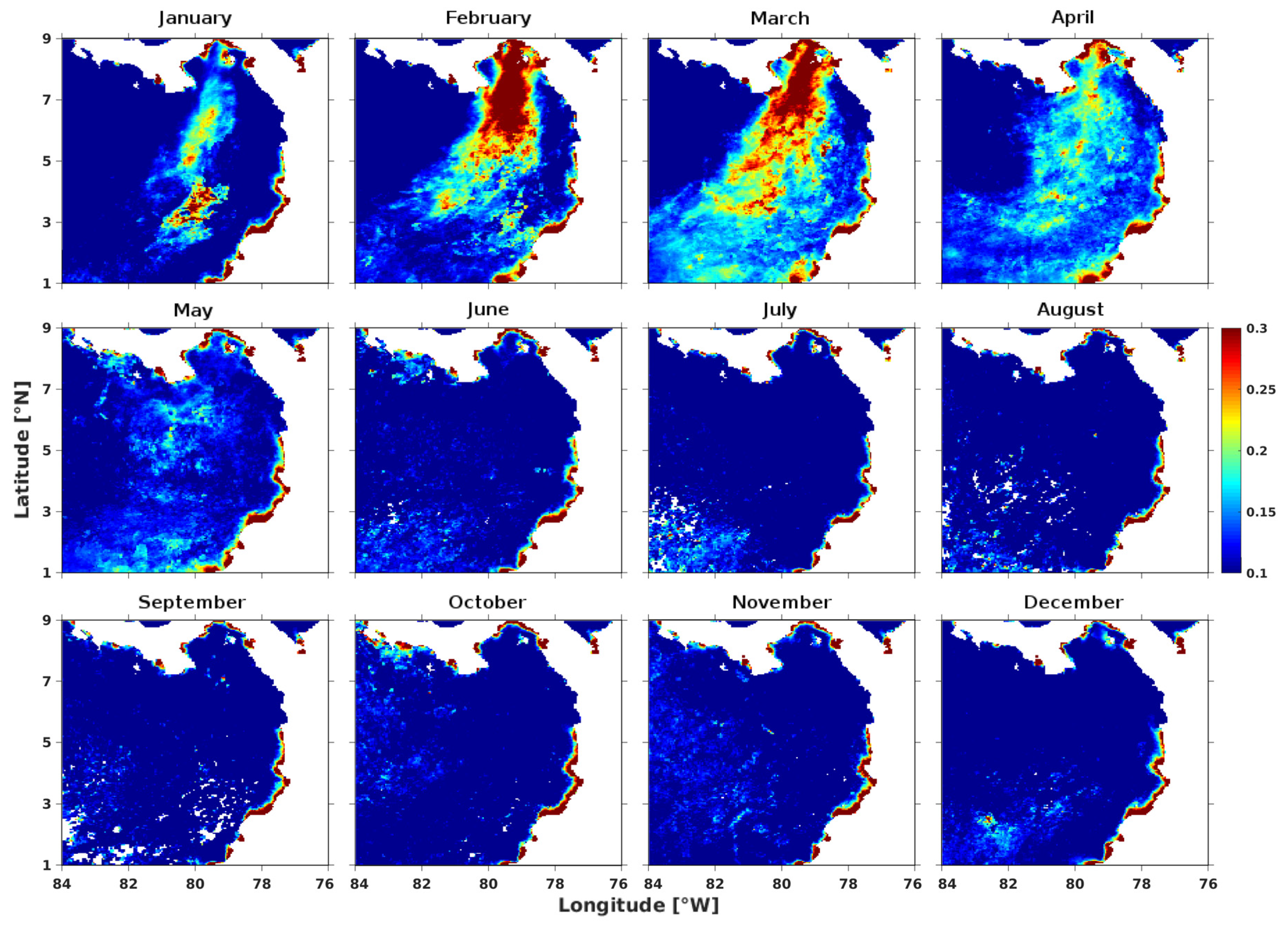
3.1. Spatio-Temporal Variability of the Annual Cycle of Chlorophyll-a

The climatological annual cycle of Chl-a revealed a seasonal signal in the oceanic zone, with the highest Chl-a concentration values from January to May (~0.5–1.5 mg m⁻³) and the lowest, from June to December (~0.25 mg m⁻³; Figure 2). In addition, the maximum Chl-a concentrations in the Gulf of Panama generated a Chl-a plume (>1 mg m⁻³), which extends southwestward into the oceanic area during January–April. By contrast, the maximum Chl-a concentrations (>2 mg m⁻³) in the PB were observed in the coastal areas of the Gulf of Panama and Gulf of Chiriqui and the coastal area off central-southern Colombia, whereas its northern coastal area showed Chl-a values similar to those of the oceanic zone (~0.5 mg m⁻³).

The Empirical Orthogonal Functions (EOFs) performed on the monthly total Chl-a values revealed a dominant signal of seasonal variation represented by the first and second modes, explaining 56% of the total variance in the annual cycle of Chl-a in the region (Figure 3). The first mode explains 38% of the Chl-a annual variability (Figure 3a,c). The annual harmonic applied to the first mode showed a marked seasonality, characterized by maximum (minimum) Chl-a values in March (September, Figure 3a), together with a maximum amplitude of the annual cycle in the Gulf of Panama and the coastal area off southern Colombia, decreasing towards the oceanic zone (Figure 3c). The second mode explained 18% of the Chl-a variability; however, its spatial structure showed a smaller amplitude of the annual cycle in the region (Figure 3d). Therefore, in terms of the temporal variability, we determined March and September as the most contrasting months for explaining the Chl-a variation in association with the environmental drivers. In terms of the spatial variability of Chl-a, we expected different behavior in the coastal areas off the Gulf of Panama and southern Colombia in comparison with the other coastal and oceanic zones in the PB region.

3.2. Spatial Characterization of the Environmental Variables in March and September

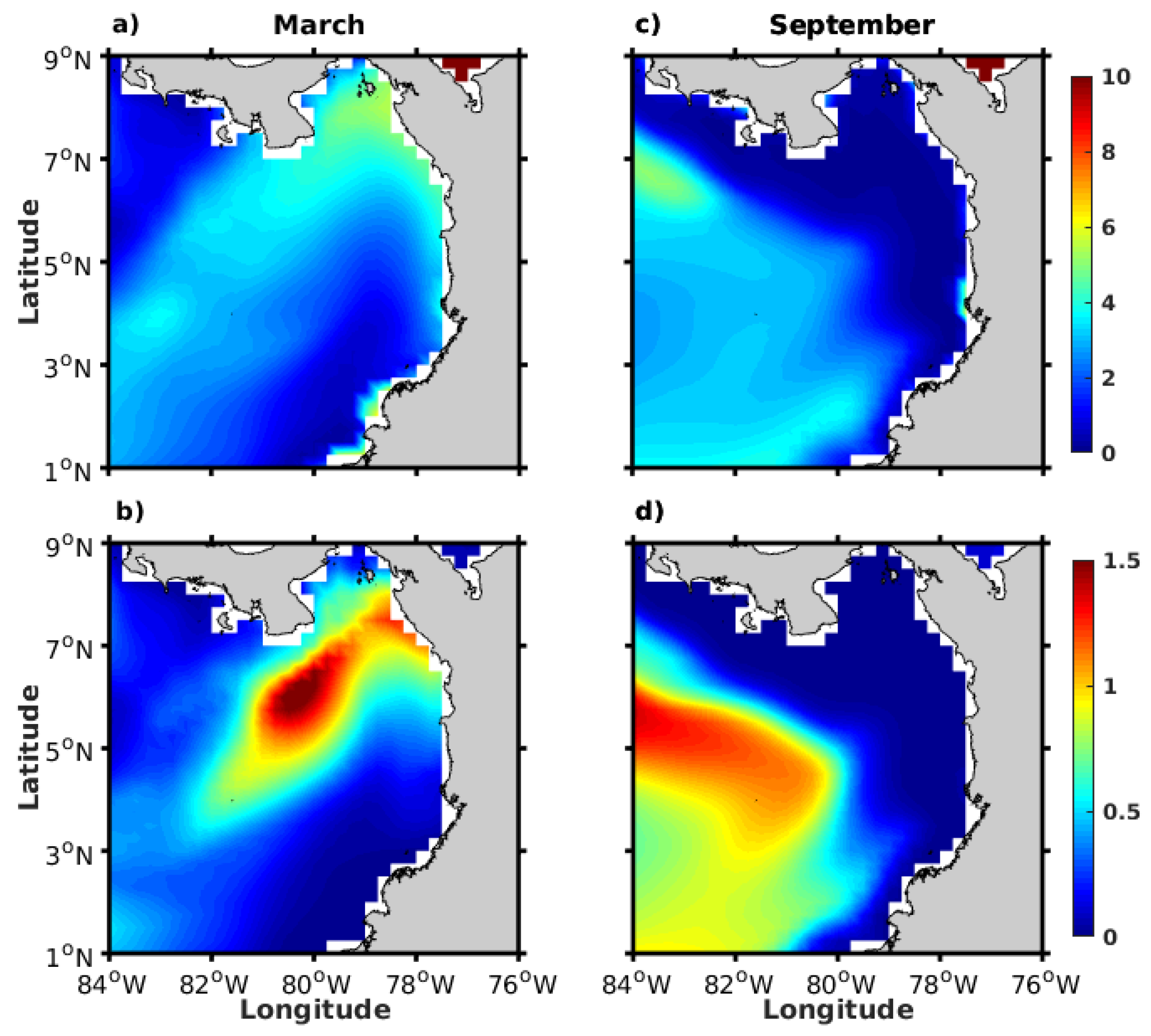
3.2.1. Wind Field and Ekman Pumping

In March, the north trade winds dominated, being intensified in Panama and generating the Panama Jet with velocities of ~5 m s⁻¹ (Figure 4a). The jet crosses the PB in a southwest direction down to ~3°N, where it splits zonally and decreases its intensity (~2 m s⁻¹). In the area between 1 and 3°N, winds from the north collided with winds from the south, deflecting east and west with lower speeds (Figure 4a). Associated with this wind pattern, the Ekman pumping showed a dipole pattern with upwelling-favorable vertical velocities on the east side (~78–80°W) and downwelling conditions on the west side (~80–84°W) (Figure 4b). The maximum Ekman pumping values (±2 m day⁻¹) were observed in the northern coastal zone of the PB (see Figure 4b, red contours). In September, the south trade winds dominated the wind field, blowing in the northeast direction and reaching higher intensities (~7 m s⁻¹) than those observed in March (Figure 4c). Positive Ekman pumping was restricted to the western part of the domain (~1–7°N, 81–84°E), reaching vertical velocities of ~1–3 m day⁻¹. Downwelling conditions were restricted to the eastern part of the domain, with maximum vertical velocities of ~ −2 m day⁻¹ in the Gulf of Chiriqui and in the southern area off Colombia (Figure 4d).

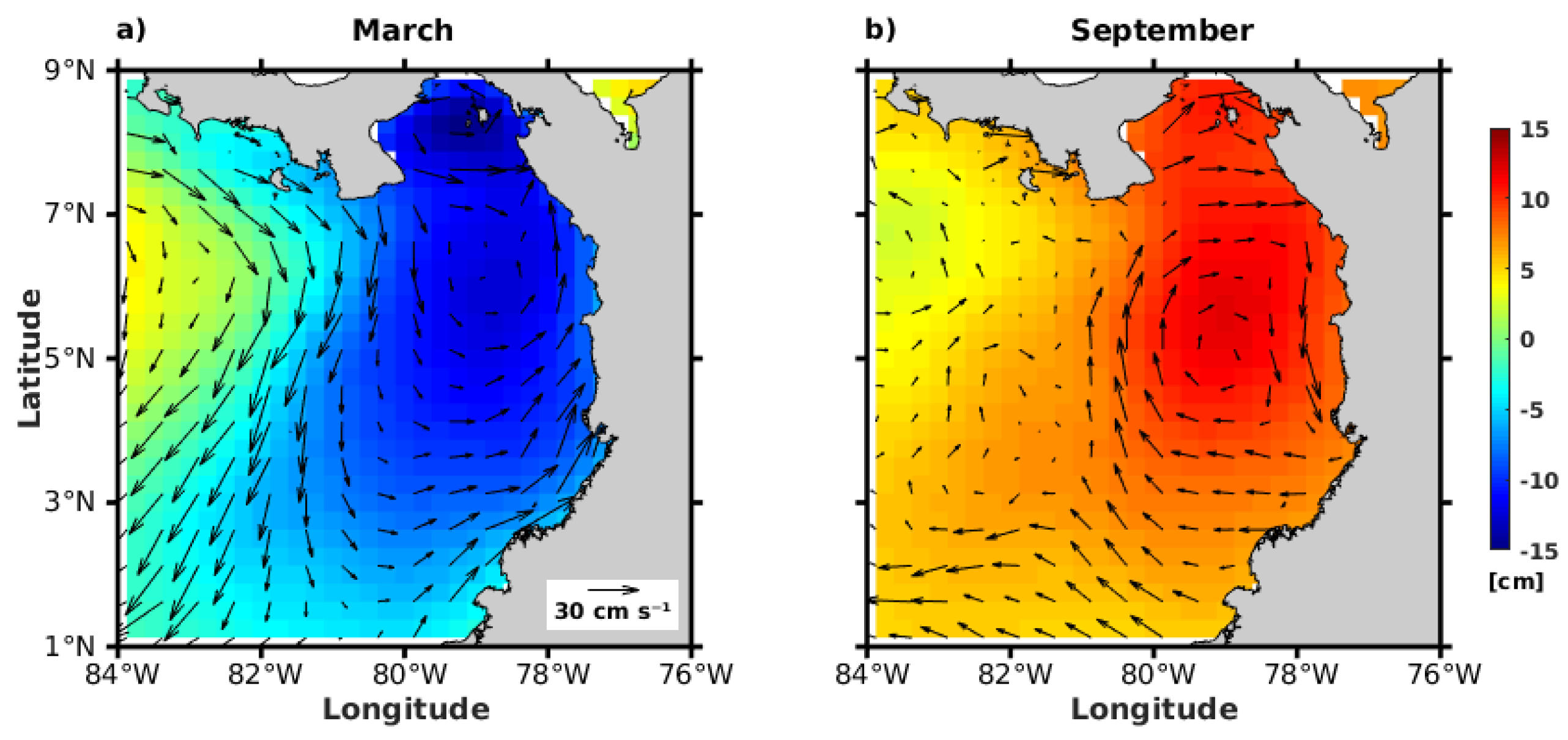
3.2.2. Geostrophic Circulation Field and Sea Level Anomalies

The Panama Jet Surface Current (PJSC) crossed the PB region in March, flowing from the Gulf of Chiriqui to the south around ~82°W (Figure 5a). On its west side, a portion of an anticyclonic gyre was observed with positive SLA values of ~5 cm (~5–7°N, 82–84°W). There were two cyclonic gyres to the east of the PJSC, one located in the Gulf of Panama (~7–9°N, 78–80°W) and the other, off the Colombian coast (~3–7°N, 78–80°W), both with negative SLA values of about −10 to −15 cm. In addition, a coastal current flowing northward along the southern Colombian margin was formed and reached the southern flank of the largest oceanic cyclonic gyre (Figure 5a). By contrast, the surface circulation field reversed in September, and an anticyclonic gyre was observed off the Colombian coast (~3–7°N, 78–80°W) with positive SLA values (~10 to 15 cm). Moreover, the cyclonic gyre in the Gulf of Panama and the anticyclonic gyre in the northwest area of the PB were no longer observed. Instead, these features were replaced by a lower intensity anticyclonic gyre centered around 4°N, 82°W, a cyclonic gyre in the northwest part of the domain (~7°N, 84°W), and a westward surface current in the southern area of the PB with a maximum speed of ~25 cm s⁻¹ (Figure 5b).

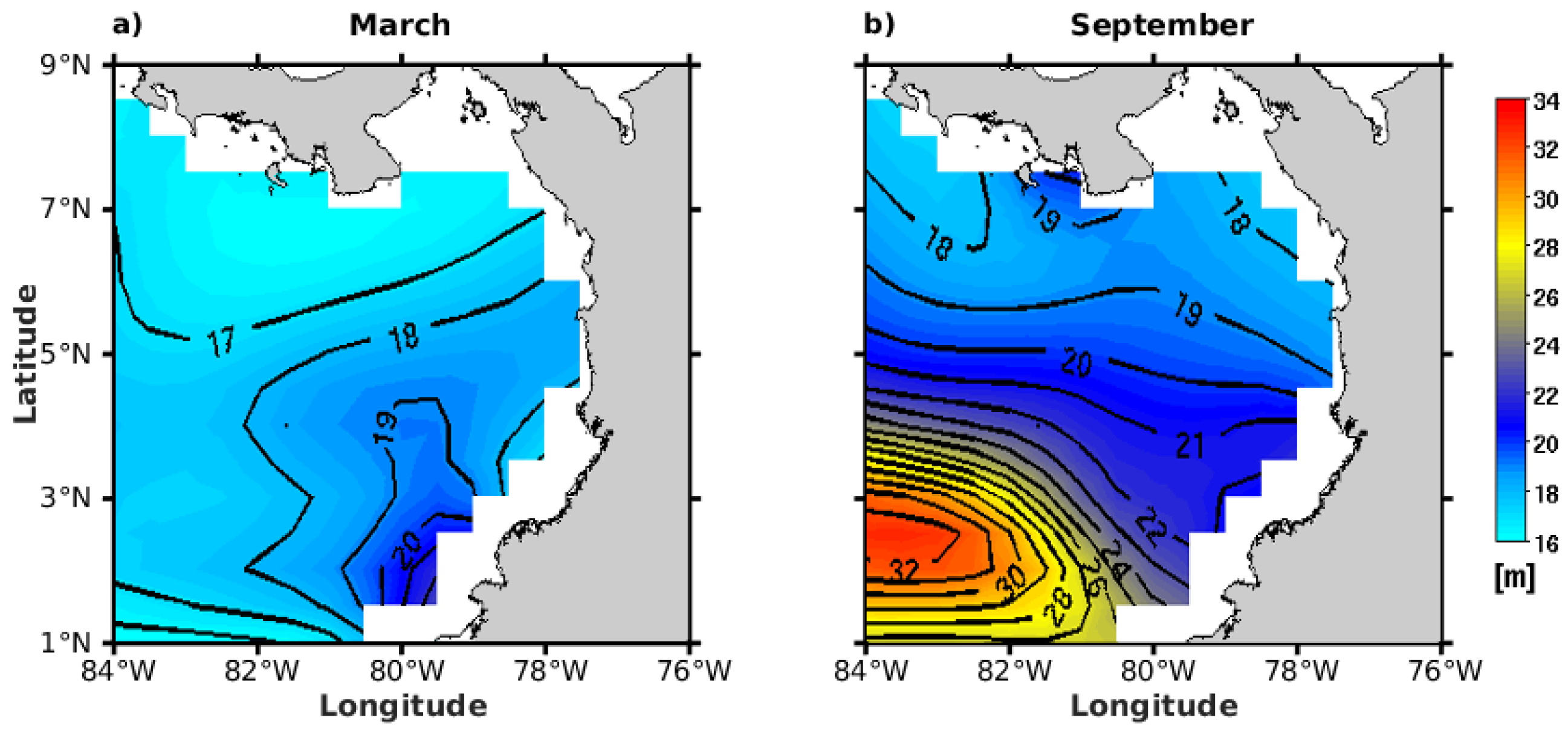
3.2.3. Mixed Layer Depth

The observed spatial variability of the MLD in the PB is shown in Figure 6. In March, the MLD was found at depths between 18 and 20 m throughout the region (Figure 6a) and was estimated at similar depths in the northern part of the domain in September (~5–8°N). However, it deepened considerably (~32 m) in the southwest corner of the PB (Figure 6b).

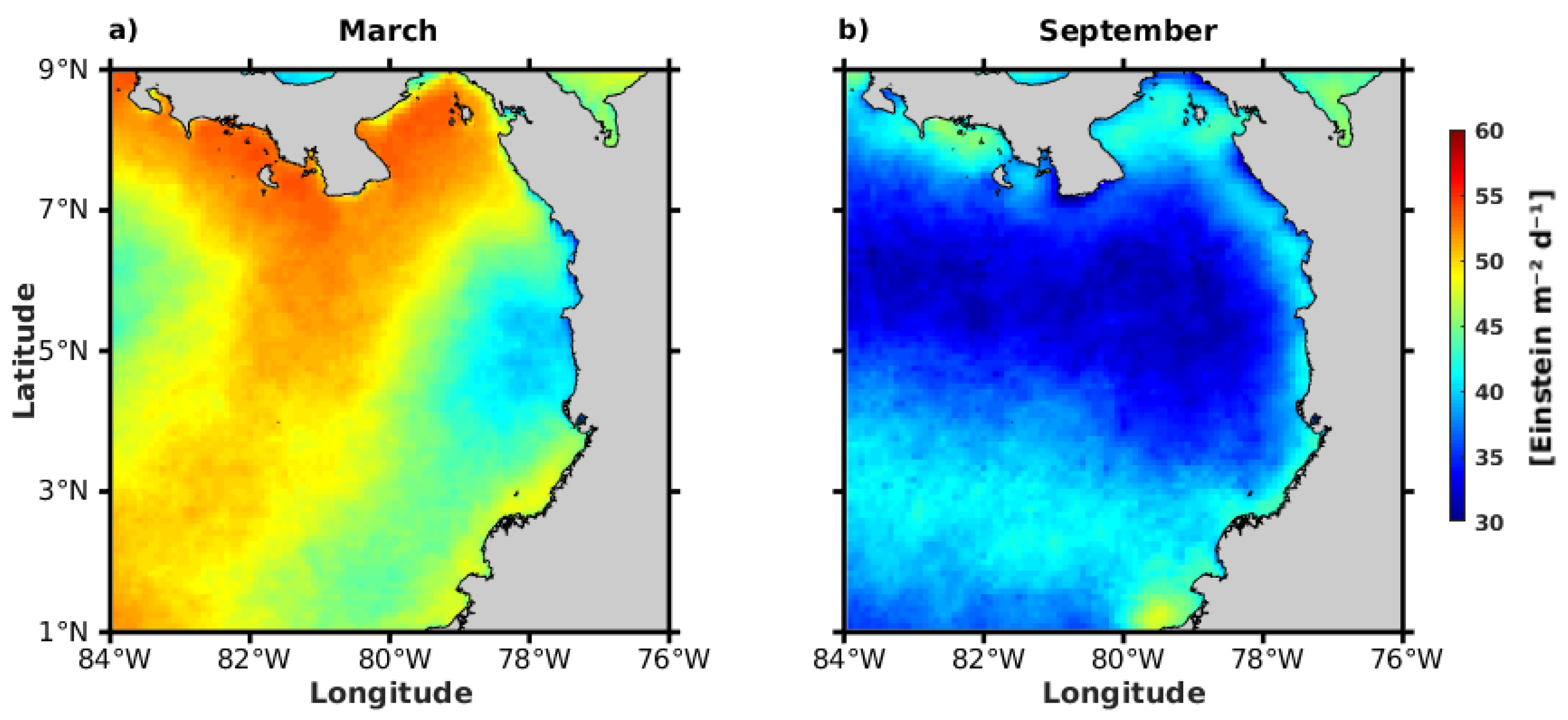
3.2.4. Photosynthetically Available Radiation

Maxima in PAR values (>50 Einstein m⁻² d⁻¹) were found across the PB from the Gulf of Panama and Chiriqui towards the southwestern area in March, while lower PAR values (<45 Einstein m⁻² d⁻¹) were observed in a coastal area off central Colombia (Figure 7a). By contrast, September represents the month with the minimum PAR values (<35 Einstein m⁻² d⁻¹) along an extended oceanic zone between 4 and 7°N. The highest PAR values during this time of the year (~45 Einstein m⁻² d⁻¹) were confined to the northern and southern edges of the study area (Figure 7b).

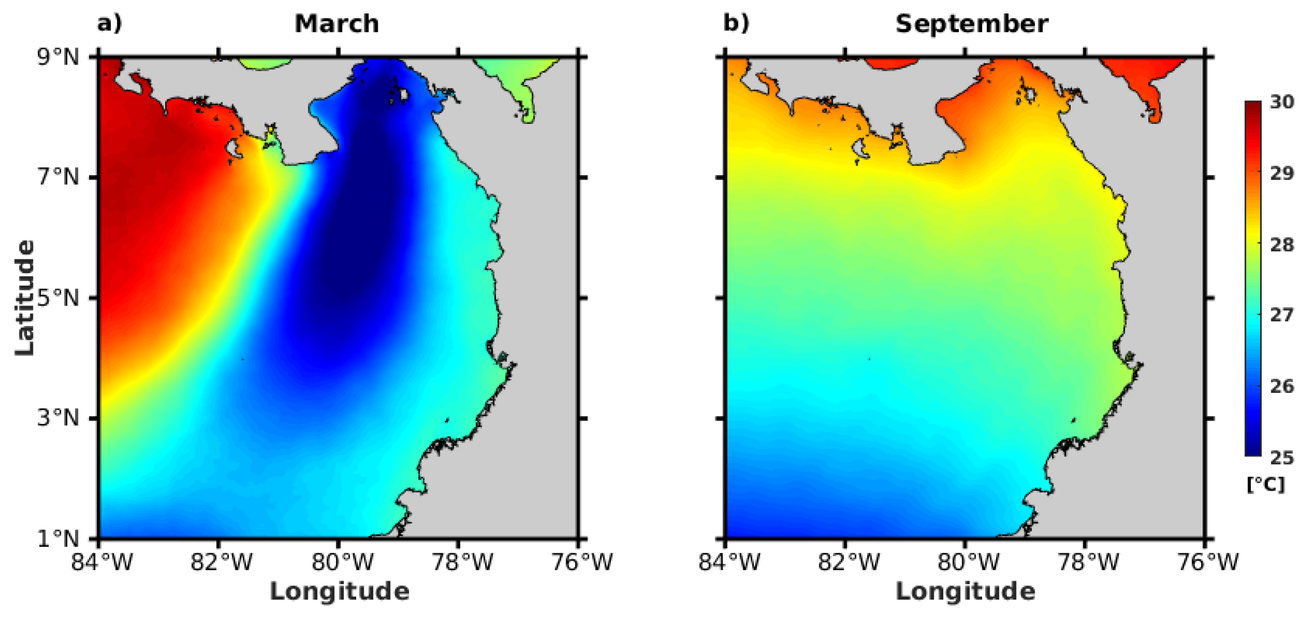
3.2.5. Sea Surface Temperature

The SST field showed a dipole pattern in March, with a low-temperature plume (25–27 °C) extending southward from the Gulf of Panama and high SST values (>28 °C) restricted to the northwest region (Figure 8a). By contrast, the SST decreased progressively towards the south in September, with values of ~28–29 °C off the Gulf of Panama to values of ~25–26 °C off southern Colombia (Figure 8b). Thus, there was a change of direction in the dominant regional SST gradient from a zonal to a meridional gradient in March and September, respectively.

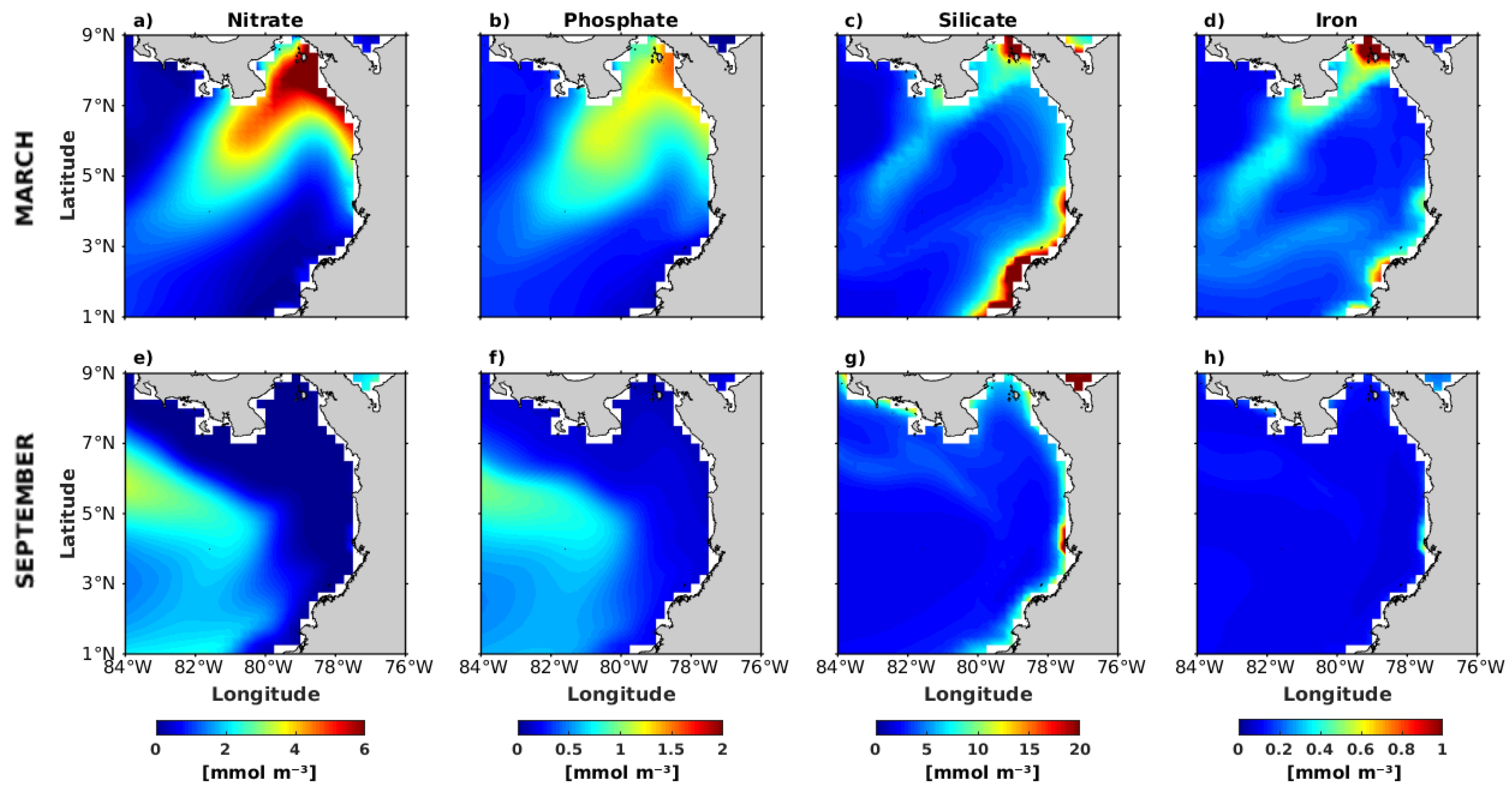
3.3. Spatial Distribution of Nutrient Content in March and September

The surface nutrient (nitrate, phosphate and silicate) and iron concentrations in March and September are shown in Figure 9. The observed nitrate/phosphate (N:P) and nitrate/silicate (N:Si) ratios are also presented for a better understanding of the nutrient distribution in the region (Figure 10). Nitrate and phosphate had similar spatial patterns, with values ranging between ~2–6 mmol m⁻³ and ~0.5–1.5 mmol m⁻³ in the northeastern part of the PB (Figure 9a,b). Silicate and iron concentrations ranged between ~5–20 mmol m⁻³ and ~0.3–1 mmol m⁻³ in the Gulf of Panama, off the Azuero peninsula, and in the oceanic region off central Colombia (Figure 9c,d). In September, nitrate and phosphate concentrations were elevated (~3 mmol m⁻³ and ~1 mmol m⁻³, respectively) over the southern oceanic area of the PB (Figure 9e,f), while the silicate concentration reached ~5–10 mmol m⁻³ in the coastal zones. The iron content was mostly depleted in the PB (Figure 9h). However, localized maxima of silicate and iron (~20 mmol m⁻³ and ~0.4 mmol m⁻³, respectively) were associated with the San Juan river discharge (Figure 9g,h, see also Appendix A). The N:P and N:Si ratios indicated deficits in nitrate (Figure 10a) and silicate (Figure 10b) across the PB, with contrasting spatial distributions in March versus September (Figure 10c,d). Whereas the deficits of nitrate and silicate were confined mostly to the northeast area in March, these were shifted to the southwestern region in September (Figure 10).

4. Discussion

4.1. Association between Chlorophyll-a and the Environmental Drivers

The climatology of the annual cycle of Chl-a revealed a seasonal pattern variation, with the highest Chl-a values observed from January to May and the lowest, from June to December, as previously reported by [30]. The PB region is characterized by having two climatic seasons, the dry (December to April) and rainy (May to November) seasons, both forced by the trade winds and the meridional migration of the ITCZ [13,36].

During the dry season, and specifically in March, the ITCZ reaches its southernmost position in the PB together with the intensification of the northeastern trade winds as they cross the Isthmus of Panama (intensification of the Panama Jet; Figure 4a), being the primary driver of the climatic seasonality in the region [11,32,34]. The wind pattern around the Panama Jet axis generates a dipole in the Ekman pumping (Figure 4b), together with a surface circulation characterized by a cyclonic gyre on the east of the Panama Jet, an anticyclonic gyre on the west, and the PJSC flowing southward along the PB (Figure 5a) [34,35,36]. The intense wind jet promotes the high availability of light by displacing the clouds across the oceanic zone (Figure 7a) [31,33], together with a cooler water tongue from the Gulf of Panama towards the south (Figure 8a) coinciding with the intensification of the upward vertical water velocities, and the maximum rise of the thermocline in the northern part of the PB [32,34]. These atmospheric and oceanographic features can promote both light availability (PAR; Figure 7a) and the input of nutrients into the upper layer, with a spatial structure as the plume of high Chl-a in March (Figure 2 and Figure 9a–d). Despite this, the low Chl-a values found in the western part of the domain can be associated with downwelling-favorable Ekman pumping velocities (Figure 4b) and the anticyclonic gyre (Figure 5a), which could locally produce a downward isopycnal displacement, modulating the phytoplankton growth rates in association with variations in the availability of nutrients and/or light with depth [59].

By contrast, the ITCZ was located in the northern part of the PB during the rainy season. This results in a shift of the wind pattern and an intensification of the southwestern trade winds as they cross the region flowing towards the continent (the Choco Jet; Figure 4c) [60]. The shift in the wind pattern leads to an Ekman pumping favorable to downwelling in the eastern half of the domain (Figure 4d), an anticyclonic oceanic gyre (also favorable to downwelling; Figure 5b), a deep mixed layer (Figure 6b), and a low nutrient content (Figure 9e–h)—altogether promoting the observed regional low Chl-a values in September (Figure 2). In addition, the deeper mixed layer over the west side of the domain (Figure 6b) could explain the low Chl-a concentrations despite having upwelling-favorable Ekman pumping velocities (Figure 4d) and a high nutrient content (Figure 9e,f). Regarding SST and PAR, the prevailing wind field enhances the north–south gradient of SST (Figure 8b) [34,60], and the greater cloud coverage decreases the light availability (Figure 7b) for phytoplankton cells to grow across the oceanic region.

Among these relationships between the environmental variables and Chl-a, the DISTLM analysis highlights different key physical drivers affecting the increase or decrease in phytoplankton biomass on a regional scale (

Table 1. Chlorophyll-a variance explained by the environmental variables in the PB for March and September. The marginal tests shows the relative contribution of each variable tested individually: SS denotes the total sum of squares of the complete multivariate data, the Pseudo-F value indicates the probability of a relationship between the Chl-a and the physical variable as a predictor, P is the p-value, and the % explained is the proportion of the variation explained by each variable. The conditional tests show the best combination of the environmental predictor variables that explain the largest amount of the variation in the response variable (Chl-a) based on the smallest value of Akaike’s information criterion (AIC). R² is the proportion of the explained variation for the model, RSS is the SS residual and No. Vars refers to the number of predictor variables used by the best solution model.

March	Variable	SS(trace)	Pseudo-F	P	% Explained
	SST	18.06	992.03	0.001	60.82
	SLA	1.59	117.87	0.001	5.35
	GC	1.44	90.68	0.001	4.87
	Wind	0.53	42.01	0.001	1.79
	Best Solution
	AICc	R2	RSS	No. Vars	Predictors
	−2794.8	0.7284	8.0623	4	SST, GC, SLA, Wind
September	Variable	SS(trace)	Pseudo-F	P	% Explained
	Wind	6.13	300.94	0.001	32.05
	PAR	4.25	310.00	0.001	22.24
	EP	0.81	68.84	0.001	4.27
	SLA	0.37	28.59	0.001	1.96
	GC	0.27	23.96	0.001	1.43
	SST	0.09	8.15	0.005	0.48
	Best Solution
	AICc	R2	RSS	No. Vars	Predictors
	−2859.4	0.6246	7.1809	6	All

Abbreviations of the physical predictor variables. SST: sea surface temperature, SLA: sea level anomaly, GC: Geostrophic circulation, PAR: photosynthetically available radiation and EP: Ekman Pumping.

). In March, the high Chl-a values were mainly explained by the SST (60.82%), whereas the low Chl-a values were better correlated with the wind field (32.05%) and light availability (22.24%) in September.

Changes in the abundance and composition of the phytoplankton community have been reported to coincide with changes in the SST along the PB, mostly related to upwelling areas and/or El Niño Southern Oscillation (ENSO) events. In neutral years or with weak to moderate ENSO conditions, the dominance of diatoms has been reported during both climatic seasons, with higher diatom abundance and higher Chl-a values during the dry season [61,62,63]. From January to March, the dominance of diatoms is mostly associated with the main oceanic and coastal upwelling areas (central oceanic region and coastal areas off southern Colombia), displaying a negative correlation with the SST; i.e., diatom abundance is high in upwelling areas with low SST values [62]. Instead, in years with the strong warm phase of ENSO (El Niño conditions), a high abundance of diatoms (e.g., Chaetoceros taciniosos, Skeletonema costatum and Dytylum brightwellii) was detected from March to April in areas with low SST values (25–26 °C), corresponding to localized upwelling zones. By contrast, under the same conditions (El Niño), an atypical dominance of dinoflagellates (e.g., Ceratium deflexum and Ceratium furca var furca) was observed from September to October, concentrated in the oceanic areas with high SST values (>27 °C) [64]. These reports indicate a relationship between the phytoplankton biomass and the community composition in association with the SST; however, the temperature was never a variable that was independent from other oceanographic processes (mainly upwelling) or ENSO events. This is also indicated in the DISTLM analysis through Akaike’s criterion, which shows that in total four predictors or physical variables (SST, SLA, geostrophic circulation, and wind) should be considered to better explain the high Chl-a concentrations in March (Table 1).

Water temperature variations may also have an impact on the ecosystem’s functioning through changes in the metabolic rates and phytoplankton cell size. Although this relationship is difficult to test, even under controlled experimental conditions, an inverse relationship between temperature and final body size has been observed, i.e., a colder temperature induces a larger cell size [65,66,67]. In March, when the DISTLM analysis indicates an important relationship between Chl-a and SST, the reported dominance of large phytoplanktonic cells in the PB [61,62,63] also suggests a higher requirement for nutrients, due to which the effect of the nutrient supply could be stronger than the temperature effect upon the phytoplankton metabolic rates. In that case, the nutrient availability can have a more significant role than temperature in controlling the efficiency of photosynthetic carbon conversion into new biomass, especially in nitrogen-limited regions [68], as is the PB (Figure 9 and Figure 10). However, we could not test these assumptions, and they should be explored in future work, preferably through determining biomass-specific carbon fixation rates under different temperatures (as the independent variable) and nutrient supply conditions. Moreover, considering that (i) variations in the tropical phytoplankton community structure are strongly linked to ENSO events, and (ii) the use of Chl-a data alone causes bias in the estimation of phytoplankton biomass, which can be misleading when the relationships between physical drivers and phytoplankton growth are evaluated [24,69].

In that sense, phytoplankton cells need to produce an amount of Chl-a in response to the nutrient content and light availability to optimize photosynthesis, but this does not necessarily imply a linear covariation between Chl-a biomass and phytoplankton carbon. For example, under stable light conditions, there is no need for the cells to produce large amounts of the energetically expensive Chl-a pigment, so the phytoplankton exploit the availability of nutrients to grow, despite the decrease in the Chl-a values. Instead, under decreasing light availability, the phytoplankton cells allocate a greater amount of the energy from the nutrients into the production of Chl-a, even though this limits their growth rate. Consequently, the use of Chl-a data alone does not necessarily take into account the physiological adjustments that phytoplankton undergo in response to changes in the environment, such as in light and nutrient conditions [70,71,72]. Future studies are encouraged, combining in situ experiments with satellite-based measurements of Chl-a and/or size-fractionated Chl-a, as well as the use of Chl-a biomass and phytoplankton carbon on both seasonal and interannual scales.

On the other hand, the association among the observed low regional Chl-a values, the wind field and the low light availability in September (Table 1) are in agreement with previous studies describing a decrement in Chl-a during the rainy season, mainly due to the weakening of the upwelling [30,32,34]. Periods with increased cloud coverage and low PAR (Figure 7b) limit the growth rates of phytoplankton cells due to the light limitation, which in the Eastern Pacific has been reported to be co-limited by macronutrients and iron [73,74], as is the case for the PB (Figure 9e–h). In addition, the DISTLM analysis also shows other four predictors to be considered to better explain the observed low Chl-a values in September, such as the Ekman pumping, SLA, geostrophic circulation and SST. In this sense, the reduction in cell size under increased temperatures could also be an adaptive response by a change in the species composition in association with resource availability [66,75]. Furthermore, the ratio of the supply to potential consumption of limiting nutrients is reduced when the temperature increases; therefore, a reduced cell size can compensate for the limitation of resources, since their uptake is more efficient by smaller cells [66,67,76].

Beside these regional relationships, we further explore the spatial Chl-a variability by dividing the PB into several subdomains in order to better understand the variability of Chl-a in the oceanic and coastal areas.

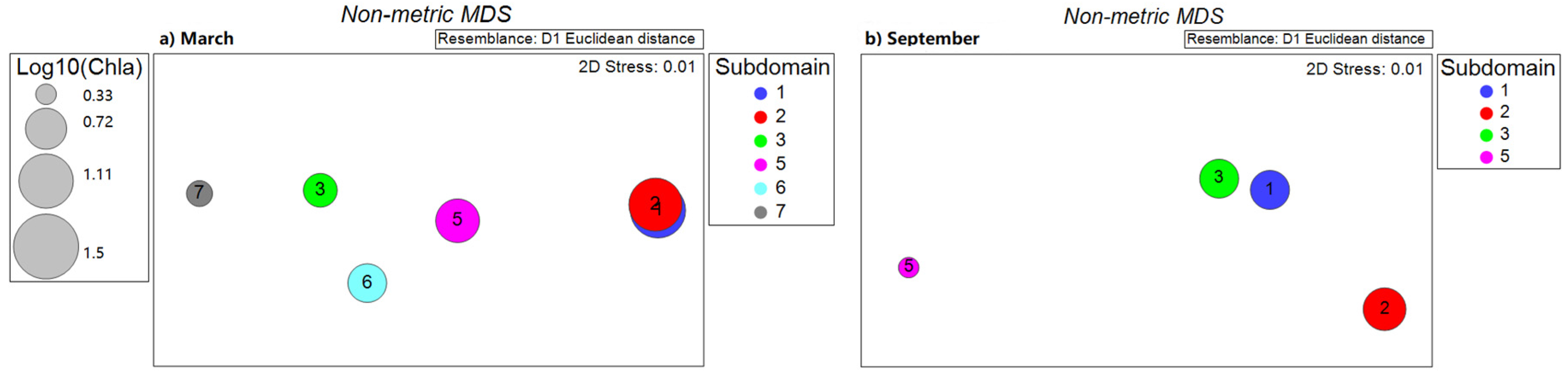
4.2. Characterization of Chlorophyll-a by Subdomains in Association with Physical Drivers and Nutrient Availability

According to bathymetry features, number of rivers and Chl-a concentration range, the PB region was divided into subdomains, seven in March and five in September (Figure 11). The coastal subdomains (1, 2, 3 and 4) remain the same for both periods, whereas the oceanic subdomains (5, 6 and 7) in March became only one (5) in September due to the homogeneity of low Chl-a values across the oceanic region.

In general, higher Chl-a values were observed in the coastal subdomains for both periods, mainly in Subdomains 1 (Gulf of Panama) and 2 (coastal area off central-southern Colombia; Figure 11), also in agreement with the spatial differences of the Chl-a values observed in the nMDS analysis (Figure 12). Note that Subdomain 4 was not included in this analysis or in the calculation of the linear Pearson correlations between Chl-a and the physical/chemical variables (

Table 2. Linear Pearson correlations between Chl-a and physical variables and nutrient content in each subdomain and for both periods (March and September).

Month	Subdomain	Mean Chl-a	n	Physical Variables						Nutrients
				SST	Wind	EP	GC	SLA	PAR	N	P	Si	Fe
March	1	1.14	28	--	--	0.42	-0.43	--	--	--	--	--	0.44
	2	1.07	26	0.51	--	--	0.52	--	--	--	--	--	--
	3	0.57	26	0.48	--	--	--	--	--	0.87	0.87	0.91	0.90
	5	0.79	318	0.72	0.73	0.12	−0.22	−0.55	0.23	0.58	0.64	0.11	--
	6	0.66	129	--	--	0.51	−0.39	−0.49	−0.46	−0.47	−0.49	0.41	0.24
	7	0.41	117	−0.95	0.93	−0.74	0.44	−0.66	0.57	0.92	0.92	0.94	0.93
September	1	0.67	28	--	0.57	--	--	--	--	--	--	--	--
	2	0.76	25	0.64	−0.79	0.42	--	--	--	--	--	--	--
	3	0.67	22	0.64	−0.57	--	0.51	--	0.51	--	--	--	--
	5	0.33	565	0.27	−0.50	−0.11	0.25	0.12	--	−0.35	−0.42	0.69	0.25

n: amount of data per subdomain. Physical variables are SST: sea surface temperature, EP: Ekman pumping, GC: geostrophic currents, SLA: sea level anomaly, and PAR: photosynthetically available radiation. Nutrients are N: nitrate, P: phosphate, Si: silicate, and Fe: Iron. The magnitude of wind and GC were used in the correlations. Only significant positive or negative correlation coefficients are displayed (p-values < 0.05).

) due to the restricted spatial coverage of this subdomain, which implies low data availability. Nonetheless, we analyzed the Chl-a variability in Subdomain 4 based on the local oceanographic processes, bathymetry and river discharges.

The PB is located in the second rainiest region of the world with maximum and minimum rainfall values in the Colombian Pacific (CP) occurring in August and January–March, whereas in Panama, these extremes occur in October and February–March, respectively [38,39]. In addition, maximum river discharges into the Gulf of Panama, the Azuero Peninsula, and the Gulf of Chiriqui occur from September to November [77]. By contrast, low river discharges are reported in northern Colombia (north of Point Arusi; Figure 1), and the highest, in the central-southern coast, with maximum values from October to November, except for the Patia and Mira rivers, with maximum discharge rates restricted to the period of March–May [49,50,78] not shown. High rainfall rates and river discharges promote the input of not only nutrients to the continental shelf but also of sediments (e.g., > 30.13 × 10⁶ tons of sediments per year in the Colombian coast) [79]. This could lead to a misinterpretation of the satellite Chl-a signal in the coastal areas due to the masking of Chl-a in high turbidity regions. The combined use of remote sensing reflectance at 645 nm (Rrs645) as a proxy for turbid plumes with high loads of sediments [80,81] and the normalized fluorescence line height (nFLH) for phytoplankton fluorescence activity [82] helped us to confirm that high phytoplankton biomass is found in the coastal areas of the Gulf of Panama and off central-southern Colombia year-round (Appendix A).

In March, the localized input of nutrients by rivers into the coastal subdomains (1 to 3) could have promoted the observed high Chl-a values, which together with the widest continental shelf could imply a longer residence time of nutrients to be used by phytoplankton in those areas (Figure 1 and Figure 9a–d). Moreover, other factors were favoring the increase in the phytoplankton signal in the coastal subdomains (see the linear correlations in Table 2). In the Gulf of Panama (Subdomain 1), the high Chl-a values were correlated with the Ekman pumping and the cyclonic gyre (Figure 4b and Figure 5a), both favorable to the upwelling of nutrients towards the upper layer, and were also positively correlated with the availability of iron (Figure 9d). In the central-southern region off Colombia (subdomain 2), the configuration of the geostrophic circulation field with the Coastal Current flowing northward (Figure 5a) probably kept the primary production restricted to the coast, together with localized upwelling centers previously reported by [30]. In the Gulf of Chiriqui (Subdomain 3), lower Chl-a values were found in comparison with those in the other coastal subdomains (1-2; Figure 12a). However, the Chl-a concentrations here appeared to be strongly associated with the availability of all nutrients (0.87 < r < 0.91; Table 2), possibly related to a localized input of nutrients by river discharges (Figure 1 and Appendix A) and/or to an advection of nutrients and Chl-a from the Gulf of Panama (closest to the Azuero Peninsula). The input of nutrients by upwelling in this area has been discarded as a dominant Chl-a driver due to a lower wind intensity during March (Figure 4a) [37]. Lastly, in the northern region off Colombia (Subdomain 4), the Chl-a signal seems to be mostly related to an advection of nutrients or Chl-a from the Gulf of Panama and from the eastern edge of the largest cyclonic gyre in the PB (Figure 5a), because other factors such as the narrow continental shelf and the absence of large rivers (Figure 1 and Appendix A) may have hindered the increase in phytoplankton biomass.

Regarding the oceanic subdomains in March, Chl-a decreased from Subdomain 5 to 7 (Figure 12a). In Subdomain 5, the Chl-a values were highly correlated to the upwelling-favorable wind field, also bringing colder deep waters and nutrients to the upper layer (Figure 4a,b, Figure 8a, and Figure 9a,b). The positive correlation values (0.58 < r < 0.64; Table 2) between Chl-a and the availability of nitrate and phosphate may indicate favorable conditions for phytoplankton growth. In Subdomain 6, Chl-a was mainly associated with the Ekman pumping favorable to upwelling although with lower intensity than in Subdomain 5 (Figure 4a), and relatively low PAR values as indicated by its negative correlation. By contrast, the lowest Chl-a values in Subdomain 7 were associated with multiple factors (Table 2), mainly the wind conditions favorable to downwelling (Figure 4a,b) and the lowest nutrient content (Figure 9a–d).

In September, lower Chl-a values were observed in all the subdomains compared to those in March, except in Subdomain 3, where the Chl-a values remained similar for both periods (Figure 12 and Table 2). In terms of the spatial variability of Chl-a by subdomain in September, Subdomains 1 and 2 show higher Chl-a values than those of Subdomains 3 to 5 (Figure 2 and Figure 12 and Table 2). In the Gulf of Panama (Subdomain 1), the high Chl-a values were strongly restricted to the coast and potentially associated with a localized input of nutrients by rivers (Figure 1 and Appendix A), which had a maximum discharge (~4500 m³ s⁻¹) from September to November [49,50]. In addition, the low nutrient content observed in this area (Figure 9e–h) could imply a faster uptake of nutrients by phytoplankton. Nonetheless, there was also a wind pattern favorable to downwelling (Figure 4c,d and Table 2), which could have contributed to the lower nutrient content and the decrease in Chl-a in the offshore area. Likewise, off central-southern Colombia (Subdomain 2), the high Chl-a values were restricted to the coast in association with high river discharges during the rainy season and the coastal signal of Ekman pumping favorable to upwelling (Figure 1 and Figure 4d and Appendix A). However, the negative correlation between Chl-a and the wind magnitude (r= −0.79, Table 2) could indicate an adverse effect on phytoplankton due to higher turbulence, not favorable for phytoplankton growth [83]. In terms of subdomains with low Chl-a in September, the absence of upwelling and elevated river discharges could limit the input of nutrients for phytoplankton growth off northern Colombia (Subdomain 4). Across the oceanic region (Subdomain 5), the low Chl-a values were associated with low PAR (Figure 7b), a deficit of silicate and a higher magnitude of wind (Figure 4c and Figure 10d and Table 2), despite the Ekman pumping pattern favorable to upwelling (Figure 4d). In the case of the Gulf of Chiriqui (Subdomain 3), the localized intense downwelling conditions (Figure 4d) could generate the decrease in Chl-a, despite the maximum river outflows reported from September to November [49,50,77].

In all subdomains and for both study periods (March and September), we highlight the physical and chemical variables that may promote the high and low Chl-a values across the PB. However, further detailed analyses are needed in order to more effectively test the sources of the nutrients (e.g., by upwelling or rivers) in the areas of high Chl-a values, as well as more frequent biological sampling (e.g., time series at fixed stations) across the region to obtain a higher spatio-temporal resolution of the phytoplankton’s responses to different oceanographic conditions. In addition, measurements focused on the phytoplankton community are needed to obtain a better picture of (i) how phytoplankton changes in association with the physical and chemical drivers, and (ii) how they adapt to the high spatio-temporal environmental variability to maintain this highly productive region, which is also characterized by high biodiversity and endemism [84,85].

4.3. Reliability of Satellite Data

The merged OC-CCI total Chl-a data product has been widely used in global and regional studies, displaying high correlation coefficient values (>0.85) and low root-mean-square errors (<0.30) between the satellite estimates and in situ measurements [86,87,88]. Besides, the fact that this product includes inter-sensor bias-corrected time series data improves the spatial and temporal coverage, maintaining rigorous standards for data quality, error characterization, and per-pixel uncertainty characterization based on its validation [44]. Future work on the study area should include in situ Chl-a data to assess the performance of this product in the PB region.

Regarding wind surface data, the V2 CCMP product is a combination of inter-calibrated wind data from satellite scatterometers (QuikSCAT and ASCAT) and microwave radiometer sensors (SSM/I, TMI and AMSR-E). Both radiometer and scatterometer data are validated against in situ information compiled from moored buoys using a variational analysis method (VAM), with the ERA-Interim reanalysis as a background input of the wind field. In general, the CCMP data are nearly unbiased relative to the assimilated wind speeds, with a root-mean-square fit of ~0.5 m s⁻¹ and a root-mean-square vector difference of ~0.8 m s⁻¹ from the assimilated QuikSCAT data, and no directional bias. However, a lower accuracy is expected at high wind speeds (>15 m s⁻¹) and under strong storm conditions. Beside this, the CCMP winds are useful in descriptions and evaluations of air–sea processes, for driving regional and large-scale ocean models, to provide reliable ocean climatologies, and oceanographic applications [89]. In terms of SLA and geostrophic currents, these products are generated by the DUACS processing system including data from a stable number of altimetry missions in order to ensure the long-term stability of the ocean observation system. The SLA product errors in the coastal areas (<200 km) are estimated at 8.2 cm²; however, higher error values could be observed in high variability coastal regions and in the retrieval of mesoscale oceanic features [90], cases in which additional criteria for data processing should be considered [88]. Furthermore, the results obtained from these products (wind field, SLA and geostrophic currents) are consistent with those previously reported in the study area through the use of other satellite databases and/or in situ data [30,32,34].

Finally, the MUR-SST analysis combines infrared satellite SST data at high (1 km; MODIS) and medium (4 to 8.8 km; AVHRR) spatial scale resolutions with microwave satellite SST data (AMSR-E, WindSat and AMSR2) in a nominal sampling of 25 km, and with global SST in situ measurements. The MUR product improves the analyzed feature resolution by one order of magnitude over most existing SST analysis products, from ~100 km down to ~10 km, and is suitable for obtaining accurate SST values displaying smaller biases (<±0.1 °C) and lower root-mean-square errors (<0.6 °C) compared with other satellite and in situ SST datasets [91].

5. Conclusions

The PB presents high Chl-a values in March, mainly related to the lowest values of the sea surface temperature. This association coincides with a seasonal wind pattern favorable to upwelling and two oceanic cyclonic gyres, both bringing colder waters and nutrients to the sunlit upper layer, favoring phytoplankton growth. Despite this, variations in the water temperature may also have an impact on phytoplankton functioning through changes in the metabolic rates and cell size, i.e., a colder temperature induces a larger cell size and therefore higher Chl-a concentrations. However, we could not test this hypothesis because the temperature was not a factor that was independent of other atmospheric or oceanic processes. By contrast, low Chl-a values in the PB were found in September in association with the seasonal shift of the wind pattern to downwelling-favorable and the low light availability. Besides this, the coastal areas displayed high Chl-a values throughout the year, mainly in the Gulf of Panama and the nearshore region off central-southern Colombia. In March, this high productivity pattern seems to be in phase with the regional patterns favorable for phytoplankton growth, whereas during the rainy season (specifically in September), the input of nutrients by river discharges, together with localized upwelling centers and the geostrophic circulation patterns, is maintaining the high Chl-a values. Although we highlight the physical and chemical variables capable of promoting high and low Chl-a values across the PB, future studies should focus on the phytoplankton community to better assess their changes, year-round, capable of sustaining the high biodiversity of the PB. Additionally, we encourage the combination of different observational (in situ and satellite data) and modeling tools to evaluate these changes, as that will also allow us to assess the phytoplankton variability in association with other spatio-temporal scale processes. We expect that this study will enable a better understanding of the productive dynamics of the PB, leading to the betterment of management decisions regarding fisheries, tourism centers and environmental policies.

References

1. Field, C.B. Primary Production of the Biosphere: Integrating Terrestrial and Oceanic Components. Science 1998, 281, 237–240. [Google Scholar] [CrossRef] [PubMed] [Green Version]
2. Sigman, D.M.; Hain, M.P. The Biological Productivity of the Ocean. Nat. Educ. 2012, 3, 1–16. [Google Scholar]
3. Falkowski, P.G.; Oliver, M.J. Mix and match: How climate selects phytoplankton. Nat. Rev. Microbiol. 2007, 5, 813–819. [Google Scholar] [CrossRef]
4. Ji, R.; Edwards, M.; MacKas, D.L.; Runge, J.A.; Thomas, A.C. Marine plankton phenology and life history in a changing climate: Current research and future directions. J. Plankton Res. 2010, 32, 1355–1368. [Google Scholar] [CrossRef] [PubMed]
5. Racault, M.F.; Le Quéré, C.; Buitenhuis, E.; Sathyendranath, S.; Platt, T. Phytoplankton phenology in the global ocean. Ecol. Indic. 2012, 14, 152–163. [Google Scholar] [CrossRef]
6. Racault, M.F.; Platt, T.; Sathyendranath, S.; Aǧirbaş, E.; Martinez Vicente, V.; Brewin, R. Plankton indicators and ocean observing systems: Support to the marine ecosystem state assessment. J. Plankton Res. 2014, 36, 621–629. [Google Scholar] [CrossRef] [Green Version]
7. Ward, B.A. Temperature-correlated changes in phytoplankton community structure are restricted to polar waters. PLoS ONE 2015, 10. [Google Scholar] [CrossRef] [Green Version]
8. Corredor-Acosta, A.; Morales, C.E.; Hormazabal, S.; Andrade, I.; Correa-Ramirez, M.A. Phytoplankton phenology in the coastal upwelling region off central-southern Chile (35°S–38°S): Time-space variability, coupling to environmental factors, and sources of uncertainty in the estimates. J. Geophys. Res. Ocean. 2015, 120, 813–831. [Google Scholar] [CrossRef]
9. Lévy, M.; Franks, P.J.; Smith, K.S. The role of submesoscale currents in structuring marine ecosystems. Nat. Commun. 2018, 9, 1–16. [Google Scholar] [CrossRef] [Green Version]
10. Salgado-Hernanz, P.M.; Racault, M.F.; Font-Muñoz, J.S.; Basterretxea, G. Trends in phytoplankton phenology in the Mediterranean Sea based on ocean-colour remote sensing. Remote Sens. Envion. 2019, 221, 50–64. [Google Scholar] [CrossRef]
11. Pennington, J.T.; Mahoney, K.L.; Kuwahara, V.S.; Kolber, D.D.; Calienes, R.; Chavez, F.P. Primary production in the eastern tropical Pacific: A review. Prog. Oceanogr. 2006, 69, 285–317. [Google Scholar] [CrossRef]
12. Chelton, D.B.; Freilich, M.H.; Esbensen, S.K. Satellite Observations of the Wind Jets off the Pacific Coast of Central America. Part I: Case Studies and Statistical Characteristics. Mon. Weather Rev. 2000, 128, 1993–2018. [Google Scholar] [CrossRef]
13. Amador, J.A.; Alfaro, E.J.; Lizano, O.G.; Magaña, V.O. Atmospheric forcing of the eastern tropical Pacific: A review. Prog. Oceanogr. 2006, 69, 101–142. [Google Scholar] [CrossRef]
14. Marrari, M.; Piola, A.R.; Valla, D. Variability and 20-Year Trends in Satellite-Derived Surface Chlorophyll Concentrations in Large Marine Ecosystems around South and Western Central America. Front. Mar. Sci. 2017, 4, 1–17. [Google Scholar] [CrossRef] [Green Version]
15. Clarke, A.J. El Niño physics and El Niño predictability. Annu. Rev. Mar. Sci. 2014, 6, 79–99. [Google Scholar] [CrossRef] [PubMed]
16. Wang, C.; Weisberg, R.H. The 1997-98 El Niño evolution relative to previous El Niño events. J. Clim. 2000, 13, 488–501. [Google Scholar] [CrossRef]
17. McPhaden, M.J.; Zebiak, S.E.; Glantz, M.H. ENSO as an integrating concept in earth science. Science 2006, 314, 1740–1745. [Google Scholar] [CrossRef] [Green Version]
18. Gierach, M.M.; Lee, T.; Turk, D.; McPhaden, M.J. Biological response to the 1997–98 and 2009–10 El Niño events in the equatorial Pacific Ocean. Geophys. Res. Lett. 2012, 39. [Google Scholar] [CrossRef]
19. Radenac, M.H.; Léger, F.; Singh, A.; Delcroix, T. Sea surface chlorophyll signature in the tropical Pacific during eastern and central Pacific ENSO events. J. Geophys. Res. Ocean. 2012, 117. [Google Scholar] [CrossRef] [Green Version]
20. Messié, M.; Chavez, F.P. A global analysis of ENSO synchrony: The oceans’ biological response to physical forcing. J. Geophys. Res. Ocean. 2012, 117. [Google Scholar] [CrossRef]
21. Racault, M.F.; Sathyendranath, S.; Menon, N.; Platt, T. Phenological responses to ENSO in the global oceans. Surv. Geophys. 2017, 38, 277–293. [Google Scholar] [CrossRef] [PubMed] [Green Version]
22. Christian, J.R.; Verschell, M.A.; Murtugudde, R.; Busalacchi, A.J.; McClain, C.R. Biogeochemical modelling of the tropical Pacific Ocean. I: Seasonal and interannual variability. Deep Sea Res. Part II Top. Stud. Oceanogr. 2001, 49, 509–543. [Google Scholar] [CrossRef]
23. Radenac, M.H.; Menkès, C.; Vialard, J.; Moulin, C.; Dandonneau, Y.; Delcroix, T.; Dupouy, C.; Stoens, A.; Deschamps, P.-Y. Modeled and observed impacts of the 1997–1998 El Niño on nitrate and new production in the equatorial Pacific. J. Geophys. Res. Ocean. 2001, 106, 26879–26898. [Google Scholar] [CrossRef] [Green Version]
24. Sharma, P.; Singh, A.; Marinov, I.; Kostadinov, T. Contrasting ENSO Types with Satellite-Derived Ocean Phytoplankton Biomass in the Tropical Pacific. Geophys. Res. Lett. 2019, 46, 5987–5996. [Google Scholar] [CrossRef] [Green Version]
25. Messié, M.; Radenac, M.H. Seasonal variability of the surface chlorophyll in the western tropical Pacific from SeaWiFS data. Deep Sea Res. Part I Oceanogr. Res. Pap. 2006, 53, 1581–1600. [Google Scholar] [CrossRef]
26. Romero-Torres, M.; Acosta, A.; Palacio-Castro, A.M.; Treml, E.A.; Zapata, F.A.; Paz-García, D.A.; Porter, J.W. Coral reef resilience to thermal stress in the Eastern Tropical Pacific. Glob. Chang. Biol. 2020, 26, 3880–3890. [Google Scholar] [CrossRef]
27. Rivera-Gómez, M.; Giraldo, A.; Lavaniegos, B.E. Structure of euphausiid assemblages in the Eastern Tropical Pacific off Colombia during El Niño, La Niña and Neutral conditions. J. Exp. Mar. Biol. Ecol. 2019, 516, 1–15. [Google Scholar] [CrossRef]
28. Wooster, W.S. Oceanographic Observations in the Panama Bight, “Askoy” Expedition, 1941. Bull. Am. Mus. Nat. Hist. 1959, 118, 113–152. [Google Scholar]
29. Spalding, M.D.; Fox, H.E.; Allen, G.R.; Davidson, N.; Ferdaña, Z.A.; Finlayson, M.; Halpern, B.S.; Jorge, M.A.; Lombana, A.; Lourie, S.A.; et al. Marine Ecoregions of the World: A Bioregionalization of Coastal and Shelf Areas. Bioscience 2007, 57, 573–583. [Google Scholar] [CrossRef] [Green Version]
30. Villegas Bolaños, N.L.; Málikov, I.; Díaz, D. Variabilidad mensual de la velocidad de surgencia y clorofila a en la región del Panama Bight. Rev. Mutis. 2016, 6, 82–94. [Google Scholar] [CrossRef] [Green Version]
31. CCCP. Compilación Oceanográfica de la Cuenca Pacífica Colombiana; Centro Control Contaminación del Pacífico, DIMAR: Cartagena, Colombia, 2002; pp. 1–124. [Google Scholar]
32. Rodríguez Rubio, E.; Stuardo, J. Variability of photosynthetic pigments in the Colombian Pacific Ocean and its relationship with the wind field using ADEOS-I data. J. Earth Syst. Sci. 2002, 111, 227–236. [Google Scholar] [CrossRef] [Green Version]
33. Poveda, G.; Mesa, O.J. La corriente de Chorro Superficial del Oeste (“del Chocó”) y otras dos corrientes de Chorro en Colombia: Climatología y variabilidad durante fases del ENSO. Rev. Acad. Colomb. Cienc. 1999, 23, 517–528. [Google Scholar]
34. Rodríguez-Rubio, E.; Schneider, W.; Abarca del Río, R. On the seasonal circulation within the Panama Bight derived from satellite observations of wind, altimetry and sea surface temperature. Geophys. Res. Lett. 2003, 30, 1–4. [Google Scholar] [CrossRef] [Green Version]
35. Willett, C.S.; Leben, R.R.; Lavín, M.F. Eddies and Tropical Instability Waves in the eastern tropical Pacific: A review. Prog. Oceanogr. 2006, 69, 218–238. [Google Scholar] [CrossRef]
36. Devis-Morales, A.; Schneider, W.; Montoya-Sánchez, R.A.; Rodríguez Rubio, E. Monsoon-like winds reverse oceanic circulation in the Panama Bight. Geophys. Res. Lett. 2008, 35, 1–6. [Google Scholar] [CrossRef]
37. D’Croz, L.; O’Dea, A. Variability in upwelling along the Pacific shelf of Panama and implications for the distribution of nutrients and chlorophyll. Estuar. Coast. Shelf Sci. 2007, 73, 325–340. [Google Scholar] [CrossRef]
38. Poveda, G.; Mesa, O.J. On the Existence of Lloró (the Rainiest Locality on Earth): Enhanced Ocean-Land-Atmosphere Interaction by a Low-Level Jet. Geophys. Res. Lett. 2000, 27, 1675–1678. [Google Scholar] [CrossRef] [Green Version]
39. CONAGUA. 2016. Available online: http://www.conagua.gob.pa/pnsh/estado-del-agua/el-agua-en-panama.html (accessed on 29 March 2019).
40. DeMaster, D.J. The Global Marine Silica Budget: Sources and Sinks. In Encyclopedia of Ocean Sciences, 3rd ed.; American Press: London, UK, 2018; pp. 1–655. [Google Scholar] [CrossRef]
41. Tyrrell, T. Redfield Ratio. In Encyclopedia of Ocean Sciences, 3rd ed.; American Press: London, UK, 2018; pp. 461–472. [Google Scholar] [CrossRef]
42. Lonsdale, P. Inflow of bottom water to the Panama Basin. Deep Sea Res. 1977, 24, 1065–1101. [Google Scholar] [CrossRef]
43. Tchantsev, V.; Cabrera-Luna, E. Algunos aspectos de investigación de la formación del régimen oceanográfico en el Pacífico colombiano. Boletín Científico CCCP 1998, 7–19. [Google Scholar] [CrossRef]
44. Sathyendranath, S.; Brewin, R.J.; Brockmann, C.; Brotas, V.; Calton, B.; Chuprin, A.; Cipollini, P.; Couto, A.B.; Dingle, J.; Doerffer, R.; et al. An Ocean-Colour Time Series for Use in Climate Studies: The Experience of the Ocean-Colour Climate Change Initiative (OC-CCI). Sensors 2019, 19, 4285. [Google Scholar] [CrossRef] [Green Version]
45. Kessler, W.S. Mean three-dimensional circulation in the northeast tropical Pacific. J. Phys. Oceanogr. 2002, 32, 2457–2471. [Google Scholar] [CrossRef] [Green Version]
46. Holte, J.; Talley, L. A new algorithm for finding mixed layer depths with applications to argo data and subantarctic mode water formation. J. Atmos. Ocean. Technol. 2009, 26, 1920–1939. [Google Scholar] [CrossRef]
47. Johnson, G.C.; Schmidtko, S.; Lyman, J.M. Relative contributions of temperature and salinity to seasonal mixed layer density changes and horizontal density gradients. J. Geophys. Res. Ocean. 2012, 117, 1–13. [Google Scholar] [CrossRef]
48. Schmidtko, S.; Johnson, G.C.; Lyman, J.M. MIMOC: A global monthly isopycnal upper-ocean climatology with mixed layers. J. Geophys. Res. Ocean. 2013, 118, 1658–1672. [Google Scholar] [CrossRef] [Green Version]
49. ETESA. 2019. Available online: https://www.hidromet.com.pa/open_data.php (accessed on 1 August 2019).
50. IDEAM. 2019. Available online: http://www.ideam.gov.co/solicitud-de-informacion (accessed on 1 September 2019).
51. Navarra, A.; Simoncini, V. A guide to Empirical Orthogonal Functions for Climate Data Analysis; Springer: London, UK, 2010; pp. 107–121. [Google Scholar] [CrossRef]
52. Garcia, C.A.; Garcia, V.M. Variability of chlorophyll-a from ocean color images in the La Plata continental shelf region. Cont. Shelf Res. 2008, 28, 1568–1578. [Google Scholar] [CrossRef]
53. Domínguez-Hernández, G.; Cepeda-Morales, J.; Soto-Mardones, L.; Rivera-Caicedo, J.P.; Romero-Rodríguez, D.A.; Inda-Díaz, E.A.; Hernández-Almeida, O.U.; Romero-Bañuelos, C. Semi-annual variations of chlorophyll concentration on the Eastern Tropical Pacific coast of Mexico. Adv. Space Res. 2020, 65, 2595–2607. [Google Scholar] [CrossRef]
54. Anderson, M.; Gorley, R.N.; Clarke, K.R. PERMANOVA+ for PRIMER. Guide to Software and Statistical Methods; PRIMER-E: Plymouth, UK, 2008. [Google Scholar]
55. Akaike, H. Information theory as an extension of the maximum likelihood principle. In International Symposium on Information Theory, 2nd ed.; Petrov, B., Caski, F., Eds.; Akademiai Kiado: Budapest, Hungary, 1973; pp. 267–281. [Google Scholar]
56. Clarke, K.R.; Gorley, R.N. PRIMER v6: User Manual/Tutorial; PRIMER-E: Plymouth, UK, 2006. [Google Scholar]
57. Minchin, P.R. An evaluation of the relative robustness of techniques for ecological ordination. In Theory and Models in Vegetation Science. Advances in Vegetation Science; Prentice, I.C., van der Maarel, E., Eds.; Springer: Dordrecht, The Netherlands, 1987; pp. 89–107. [Google Scholar]
58. Legendre, P.; Legendre, L. Numerical Ecology, 3rd ed.; Elsevier: Amsterdam/Dordrecht, The Netherlands, 2012; pp. 512–519. [Google Scholar]
59. McGillicuddy, D., Jr. Mechanisms of physical-biological-biogeochemical interaction at the oceanic mesoscale. Annu. Rev. Mar. Sci. 2016, 8, 125–159. [Google Scholar] [CrossRef] [Green Version]
60. Rueda, Ó.; Poveda, G. Variabilidad espacial y temporal del Chorro del Chocó y su efecto en la hidroclimatología de la región del Pacífico colombiano. Meteorol. Colomb. 2006, 10, 132–145. [Google Scholar]
61. Ramírez, D.G.; Giraldo, A.; Tovar, J. Producción primaria, biomasa y composición taxonómica del fitoplancton costero y oceánico en el Pacífico colombiano (septiembre-octubre 2004). Investig. Mar. 2006, 34, 211–216. [Google Scholar] [CrossRef] [Green Version]
62. Sogamoso, E.A.; Rubio, E.R.; Galeano, A.M. Distribución, abundancia y composición del fitoplancton y condiciones ambientales en la cuenca Pacífica colombiana, durante enero-febrero de 2007. Boletín Científico CCCP 2008, 15, 105–122. [Google Scholar] [CrossRef] [Green Version]
63. INVEMAR-ANH. Especies, Ensamblajes y Paisajes de los Bloques Marinos Sujetos a Exploración de Hidrocarburos; Informe de actividades INVEMAR-ANH Fase III-Pacífico Caracterización de la megafauna y el plancton del Pacífico Colombiano: Santa Marta, Colombia, 2010; p. 226. [Google Scholar]
64. Castillo, F.A.; Vizcaíno, Z. Los indicadores biológicos del fitoplancton y su relación con el fenómeno de El Niño 1991-92 en el Pacífico colombiano. Bol. Cient. Cioh. 1992, 13–22. [Google Scholar] [CrossRef]
65. Montagnes, D.J.; Franklin, M. Effect of temperature on diatom volume, growth rate, and carbon and nitrogen content: Reconsidering some paradigms. Limnol. Oceanogr. 2001, 46, 2008–2018. [Google Scholar] [CrossRef] [Green Version]
66. Atkinson, D.; Ciotti, B.J.; Montagnes, D.J. Protists decrease in size linearly with temperature: Ca. 2.5% C−1. Proc. R. Soc. Lond. (Boil.) 2003, 270, 2605–2611. [Google Scholar] [CrossRef] [Green Version]
67. Marañón, E.; Steele, J.; Thorpe, A.; Turekian, K. Phytoplankton size structure. In Elements of Physical Oceanography: A Derivative of the Encyclopedia of Ocean Sciences, 2nd ed.; Academic Press: Washington, WA, USA, 2009; pp. 1–85. [Google Scholar]
68. Marañón, E.; Lorenzo, M.P.; Cermeño, P.; Mouriño-Carballido, B. Nutrient limitation suppresses the temperature dependence of phytoplankton metabolic rates. ISME J. 2018, 12, 1836–1845. [Google Scholar] [CrossRef] [Green Version]
69. Kruskopf, M.; Flynn, K.J. Chlorophyll content and fluorescence responses cannot be used to gauge reliably phytoplankton biomass, nutrient status or growth rate. New Phytol. 2006, 169, 525–536. [Google Scholar] [CrossRef]
70. Bellacicco, M.; Volpe, G.; Colella, S.; Pitarch, J.; Santoleri, R. Influence of photoacclimation on the phytoplankton seasonal cycle in the Mediterranean Sea as seen by satellite. Remote Sens. Environ. 2016, 184, 595–604. [Google Scholar] [CrossRef]
71. Halsey, K.H.; Jones, B.M. Phytoplankton strategies for photosynthetic energy allocation. Annu. Rev. Mar. Sci. 2015, 7, 265–297. [Google Scholar] [CrossRef]
72. Behrenfeld, M.J.; Boss, E.; Siegel, D.A.; Shea, D.M. Carbon-based ocean productivity and phytoplankton physiology from space. Glob. Biogeochem. Cycles 2005, 19, GB1006. [Google Scholar] [CrossRef]
73. Hopkinson, B.M.; Barbeau, K.A. Interactive influences of iron and light limitation on phytoplankton at subsurface chlorophyll maxima in the eastern North Pacific. Limnol. Oceanogr. 2008, 53, 1303–1318. [Google Scholar] [CrossRef] [Green Version]
74. Mahadevan, A. The impact of submesoscale physics on primary productivity of plankton. Annu. Rev. Mar. Sci. 2016, 8, 161–184. [Google Scholar] [CrossRef] [PubMed] [Green Version]
75. Atkinson, D. Temperature and organism size: A biological law for ectotherms? Adv. Ecol. Res. 1994, 25, 1–58. [Google Scholar] [CrossRef]
76. Woods, H.A. Egg-mass size and cell size: Effects of temperature on oxygen distribution. Am. Zool. 1999, 39, 244–252. [Google Scholar] [CrossRef]
77. Milliman, J.D.; Farnsworth, K.L. River Discharge to the Coastal Ocean. A Global Synthesis, 1st ed.; Cambridge University Press: Cambridge, UK, 2011; pp. 1–384. [Google Scholar]
78. Restrepo, J. Aporte de caudales de los ríos Baudó, San Juan, Patía y Mira a la cuenca Pacífica colombiana. Boletín Científico CCCP 2006, 13, 17–32. [Google Scholar] [CrossRef]
79. Restrepo, J.D.; Kjerfve, B. Environmental Geochemistry in Tropical and Subtropical Environments. Environmental Science. In The Pacific and Caribbean Rivers of Colombia: Water Discharge, Sediment Transport and Dissolved Loads; Drude de Lacerda, L., Santelli, R.E., Duursma, E.K., Abrão, J.J., Eds.; Springer: Berlin/Heidelberg, Germany, 2004; pp. 169–187. [Google Scholar] [CrossRef]
80. Aurin, D.; Mannino, A.; Franz, B. Spatially resolving ocean color and sediment dispersion in river plumes, coastal systems, and continental shelf waters. Remote Sens. Environ. 2013, 137, 212–225. [Google Scholar] [CrossRef] [Green Version]
81. Saldías, G.S.; Largier, J.L.; Mendes, R.; Pérez-Santos, I.; Vargas, C.A.; Sobarzo, M. Satellite-measured interannual variability of turbid river plumes off central-southern Chile: Spatial patterns and the influence of climate variability. Prog. Oceanogr. 2016, 146, 212–222. [Google Scholar] [CrossRef]
82. Behrenfeld, M.J.; Westberry, T.; Boss, E.; O’Malley, R.; Siegel, D.; Wiggert, J.D.; Franz, B.; Feldman, G.; Doney, S.; Moore, J.; et al. Satellite-Detected Fluorescence Reveals Global Physiology of Ocean Phytoplankton. Biogeosciences 2009, 6, 779–794. [Google Scholar] [CrossRef] [Green Version]
83. Yokomizo, H.; Botsford, L.W.; Holland, M.D.; Lawrence, C.A.; Hastings, A. Optimal wind patterns for biological production in shelf ecosystems driven by coastal upwelling. Theor. Ecol. 2010, 3, 53–63. [Google Scholar] [CrossRef] [Green Version]
84. Miloslavich, P.; Klein, E.; Díaz, J.M.; Hernandez, C.E.; Bigatti, G.; Campos, L.; Artigas, F.; Castillo, J.; Penschaszadeh, P.E.; Neill, P.E.; et al. Marine biodiversity in the Atlantic and Pacific coasts of South America: Knowledge and gaps. PLoS ONE 2011, 6, e14631. [Google Scholar] [CrossRef] [PubMed] [Green Version]
85. Zapata, F.A.; Ross Robertson, D. How many species of shore fishes are there in the Tropical Eastern Pacific? J. Biogeogr. 2007, 34, 38–51. [Google Scholar] [CrossRef]
86. Brewin, R.J.; Sathyendranath, S.; Jackson, T.; Barlow, R.; Brotas, V.; Airs, R.; Lamont, T. Influence of light in the mixed-layer on the parameters of a three-component model of phytoplankton size class. Remote Sens. Envion. 2015, 168, 437–450. [Google Scholar] [CrossRef]
87. Brewin, R.J.; Ciavatta, S.; Sathyendranath, S.; Jackson, T.; Tilstone, G.; Curran, K.; Airs, R.L.; Cummings, D.; Brotas, V.; Organelli, E.; et al. Uncertainty in ocean-color estimates of chlorophyll for phytoplankton groups. Front. Mar. Sci. 2017, 4, 104. [Google Scholar] [CrossRef] [Green Version]
88. Corredor-Acosta, A.; Morales, C.E.; Brewin, R.J.; Auger, P.A.; Pizarro, O.; Hormazabal, S.; Anabalón, V. Phytoplankton size structure in association with mesoscale eddies off central-southern Chile: The satellite application of a phytoplankton size-class model. Remote Sens. 2018, 10, 834. [Google Scholar] [CrossRef] [Green Version]
89. Atlas, R.; Hoffman, R.N.; Ardizzone, J.; Leidner, S.M.; Jusem, J.C.; Smith, D.K.; Gombos, D. A cross-calibrated, multiplatform ocean surface wind velocity product for meteorological and oceanographic applications. Bull. Am. Meteor. Soc. 2011, 92, 157–174. [Google Scholar] [CrossRef]
90. ECMWF Copernicus, Product Quality Assessment Report, Sea Level. Available online: http://datastore.copernicus-climate.eu/documents/satellite-sea-level/D2.SL.2-v1.1_PQAR_of_v1DT2018_SeaLevel_products_v2.2.pdf (accessed on 19 June 2020).
91. Chin, T.M.; Vazquez-Cuervo, J.; Armstrong, E.M. A multi-scale high-resolution analysis of global sea surface temperature. Remote Sens. Environ. 2017, 200, 154–169. [Google Scholar] [CrossRef]
Figure 1. Study area of Panama Bight (1–9°N, 76–84°W; red rectangle) in the Eastern Tropical Pacific region. Bathymetry features (in color), main rivers (R1: Chiriqui, R2: Fonseca, R3: Santa Maria, R4: Tuira, R5: Baudo, R6: San Juan, R7: Naya, R8: Micay, R9: Patia, R10: Mira) and submarine depressions (G1: Yurupar, G2: Guanibos, G3: Omagua, G4: Yaquina) are specified for the study area enclosed in a red box.
Remotesensing 12 02150 g001
Figure 2. Monthly mean climatology of total chlorophyll-a (Chl-a) in the Panama Bight for the period of January 2002 to December 2016. The Chl-a is represented by a color scale.
Remotesensing 12 02150 g002
Figure 3. Principal two Empirical Orthogonal Function (EOF) spatio-temporal modes of the climatological annual cycle of the total Chl-a in the Panama Bight region. (a,b) Annual harmonics of the temporal EOF modes, and (c,d) corresponding spatial EOF modes.
Remotesensing 12 02150 g003
Figure 4. Climatology (2002–2016) of wind velocity (top panels) and Ekman pumping (bottom panels) for (a,b) March and (c,d) September. Red shading represents the regions of upward Ekman velocities (upwelling), and blue shading indicates downward velocities (downwelling). The gray contours denote where vertical velocities are equal to zero.
Remotesensing 12 02150 g004
Figure 5. Climatology (2002–2016) of surface currents (black vectors) and sea level anomalies (in color scale) for (a) March and (b) September. Red (blue) shading represents the regions with sea level anomalies above (below) the regional average.
Remotesensing 12 02150 g005
Figure 6. Climatology (2002–2016) of the mixed layer depth (in color scale) for (a) March and (b) September. Gray (dark red) shading represents the regions with a shallow (deep) mixed layer.
Remotesensing 12 02150 g006
Figure 7. Climatology (2002–2016) of the photosynthetically available radiation (in color scale) for (a) March and (b) September. Red (blue) shading represents regions with high (low) photosynthetically available radiation.
Remotesensing 12 02150 g007
Figure 8. Climatology (2002–2016) of sea surface temperature (in color scale) for (a) March and (b) September. Red (blue) shading represents the regions with high (low) sea surface temperature.
Remotesensing 12 02150 g008
Figure 9. Climatology (2002–2016) of surface nutrient concentrations (in color scale) in the Panama Bight (PB) during March (top panels) and September (bottom panels). Red (blue) shading represents the regions with high (low) nutrient.
Remotesensing 12 02150 g009
Figure 10. Spatial distribution of the nitrate/phosphate and nitrate/silicate ratios (in color scale) in the PB for (a,b) March and (c,d) September. In the case of the nitrate/phosphate ratio (a and c), the red color indicates deficit of nitrate, whereas in the case of the nitrate/silicate ratio (b and d), the red color indicates deficit of silicate.
Remotesensing 12 02150 g010
Figure 11. Climatology (2002–2016) of Chl-a (in color scale) for (a) March and (b) September. The black contours and numbers denote the areas for each subdomain.
Remotesensing 12 02150 g011
Figure 12. Spatial differences of Chl-a among subdomains according to the non-metric multidimensional scaling ordination (nMDS) analysis for (a) March and (b) September. Not enough Chl-a data were available to include Subdomain 4. Chl-a units in (mg m−3).
Remotesensing 12 02150 g012