Numerical Investigation of Turbulent Heat Transfer Properties at Low Prandtl Number

Introduction

The sodium-cooled fast reactor (SFR), which is one of the new generation of nuclear power plant designs, has been considered to be one of the most promising candidates for meeting the goal declared by the Generation IV International Forum (GIF) (Sun, 2012). The pitch between neighboring fuel rods in the design of the fuel assembly is usually very small due to the good thermal conductivity of liquid sodium. A small change of flow area caused by corrosive products may have a significant influence on coolant temperature and threaten the integrity of the fuel assembly. Hence, the thermal hydraulics of liquid sodium have drawn a lot of attention. It is believed that turbulent heat transfer in the liquid sodium, which is a low-Prandtl fluid, is an extremely complex phenomenon. Due to a lack of detailed knowledge about the heat transfer process, turbulent modeling of low-Prandtl number fluid is still quite limited.

In the past few decades, a lot of effort has been devoted to investigating the flow and heat transfer properties of liquid sodium (Schumm et al., 2016; Da Vià and Manservisi, 2019). A lot of work, including both experimental and numerical studies, has been carried out to provide information on heat transfer in liquid sodium. In these studies, the sodium flow inside a 7-pin rod bundle with wire-wrapped spacers was experimentally measured by Lorenz and Ginberg (1977). The temperature distributions obtained can be employed for the validation calculations of numerical configuration. Moreover, Bogoslovskaya et al. (2000) investigated the integral mixing factors between neighboring sub-channels based on the measurement of the velocity distribution surrounding fuel pins in which the electrical conductivity of liquid metal was employed. Because sodium coolant is a potential fire hazard, experimental data of liquid sodium is still quite limited. More recently, experimental study of lead-bismuth eutectic, which is another low Prandtl fluid, has become much more popular (Pacio et al., 2016). However, it is almost infeasible to provide detailed profiles of flow and heat transfer properties inside the rod bundle of an SFR with standard measurement devices. Hence, accurate modeling of turbulent heat transfer in liquid sodium remains a great challenge due to the lack of information about the complex mechanism involved.

With increasing computer power, the employment of the CFD approach has gained considerable attention. If employing the commonly used eddy diffusivity approach, it is necessarily important to clearly clarify the influence from the turbulent Prandtl number. In this classical approach, a turbulent Prandtl number which is equal to unity or close to unity fails to accurately predict the heat transfer, especially for liquid sodium (Cheng and Tak, 2006a; Grotzbach, 2013). Several models that aim at solving this problem have been proposed to estimate the turbulent Prandtl number for low-Prandtl fluids over several decades (Kays, 1994; Churchill, 2002). The turbulent Prandtl number is treated as a function of the Reynolds number or Peclet number. Based on it, a strong circumferential non-uniformity of heat transfer in bare rod bundles can be found in the numerical results of liquid metal. However, it has been found that a uniform profile of the turbulent Prandtl number is not suitable to describe the profile of turbulent heat flux and fails to accurately predict the profile of turbulent heat flux, especially in the near-wall region (Duponcheel et al., 2014). The value of the turbulent Prandtl number in the near-wall region is much larger than that in the channel center. In order to circumvent the drawbacks of the eddy diffusivity approach, the transport equation of the turbulent heat flux is carefully analyzed based on the assumption of fully developed flow and local equilibrium, and the algebraic heat flux model (AFM) is obtained. This model is believed to be suitable for anisotropic and buoyant flows and adapted to liquid metal convection (Grotzbach, 2013). An additional value named temperature variance is introduced in the model, and a large number of closures appear to evaluate several coefficients used in this model (Kenjeres et al., 2005; Shams et al., 2014). These coefficients are usually calibrated based on experimental data or DNS data. As discussed above, statistical analyses of low-Prandtl fluid are not quite sufficient, and hence consideration of the modeling of turbulent heat flux, which is necessary for the analysis of heat transfer properties of liquid sodium, is still limited.

This paper assesses the turbulent heat flux of turbulent convection at extremely low Pr. The object of the current work is to propose a more accurate closure to estimate the coefficient used in an AFM model that is more suitable for low-Prandtl fluids. Constant thermo-physical properties are assumed, and buoyancy is accounted for in the momentum equation using the Boussinesq assumption. Due to a lack of DNS and experimental data for liquid sodium, new reference results were obtained by performing a wall-resolved Large-Eddy Simulation of turbulent channel flows at Pr = 0.005. The Reynolds number was varied over a wide range to consider its influence on the turbulent heat flux. Based on the proposed results of the LES model, the algebraic turbulent heat flux model is first assessed against the LES data for a channel flow. The coefficients employed in this model are then further calibrated to reproduce the turbulent properties of liquid sodium. The optimized coefficients may provide a better prediction accuracy for application to the convection flow regime in fuel assemblies of SFRs.

Numerical Models

LES Model

In the current study, an LES model is chosen to predict the turbulence properties of the flow field. The basic equations of the LES model were first formulated by Smagorinsky (1963). With the filtering process, the incompressible Navier-Stokes equations were filtered to separate the small scales from the large scales of motion, as shown below:

where $\tilde{\text{U}}=({\tilde{U}}_x,{\tilde{U}}_y,{\tilde{U}}_z)$ is the filtered velocity field. $\tilde{p}$ and $\tilde{T}$ are the filtered pressure and temperature, respectively. F stands for the body force $F=\beta (\tilde{T}-T_m)g$, in which β is the thermal expansion ratio and T_m = (T_h + T_c)/2 is the mean temperature. α stands for the thermal diffusivity. The term τ_sgs is known as the sub-grid scale stress (SGS), which reflects the effect from the sub-grid part of the velocity field on the resolved field through the sub-grid scale model. The components of sub-grid scale stress are evaluated as follows:

In order to close the modeling, sub-grid scale eddy-viscosity ν_sgs is required. In the literature, a lot of research has been carried out to propose different models to evaluate its value. The WALE model (Nicoud and Ducros, 1999), which includes the effects from both the strain and the rotation rate of the smallest resolved turbulent fluctuations based on the square of the velocity gradient tensor, is employed in the current study.

The subject of interest is the fully developed turbulent flow of a low-Prandtl number flow through a heated channel with fixed heat flux at the walls. By feeding the outlet flow back to the inlet boundary, a fully developed flow field in a channel with a cyclic boundary condition is employed in the simulation. The modified variable Θ is then introduced to obtain a time-averaged profile of temperature in the simulation domain as:

where the gradient $\frac{d{T}_w}{dx}$ stands for the temperature increase in the periodic streamwise direction (x) due to the mean uniform heat flux q_w. Its value is calculated as:

where δ stands for the half-width of the channel, C_p is the heat capacity, and ${\overline{U}}_b$ is the bulk velocity.

With the introduction of Θ, the energy equation is modified as:

In the current study, all of the governing equations are integrated into the three-dimensional finite-volume CFD platform OpenFOAM, which is constituted by a large base library and offers the core capabilities of dynamic mesh, automatic parallelization, several generally physical models, etc.

A transient solver proposed by OpenFOAM, “buoyantPimpleFOAM,” is employed to predict buoyant, turbulent flow of incompressible fluid for heat transfer. The PISO algorithm is used to solve Navier-Stokes equations. Limited linear differencing schemes are employed for approximating the convective terms to maintain second-order accuracy. Linear, linear corrected, backward and corrected schemes are employed for the gradient term, diffusive term, time derivation, and surface gradient term, respectively. The mean profiles of temperature and velocity were obtained based on the functions provided by OpenFOAM. The arithmetic mean is calculated by:

The prime-squared mean is calculated by:

Algebraic Turbulent Heat Flux Model

Analogous to the analysis of Reynolds stress, if applying the Reynolds decomposition to the energy transport equation, turbulent heat flux $\overline{u_i\theta }$ appears in the time-averaged form of the energy equation. In the past few decades, different models have been proposed to estimate its value based on different assumptions, such as the Simple Gradient Diffusion Hypothesis (SGDH) model and the General Gradient Diffusion Hypothesis (GGDH) model (Xiong and Cheng, 2014). In these two models, turbulent heat flux is proportional to the turbulent viscosity or Reynolds stress without considering the influence of energy equilibrium. These models may not be applicable for flows in which buoyancy has to be considered. Hence, an AFM model is proposed to estimate turbulent heat flux with consideration of buoyancy force. The resulting algebraic expression has the following form (Kenjereš and Hanjalić, 2000):

where a_ij is estimated based on the Reynolds stress as: $a_{ij}=\overline{u_i{u}_j}/3-2{\delta }_{ij}/3$. The first three terms on the right-hand side of Equation 10 consider the influences of temperature gradient, velocity gradient, and buoyancy, respectively. It should be noted that the AFM model involves the temperature variance, which is unknown. An equation is introduced to solve its value:

in which $P_{tt}=\overline{u{u}_i\theta }/\frac{d\overline{\Theta }}{d{x}_i}$ and ${\epsilon }_{tt}=\frac{\epsilon \theta }{2kR}$.

In the past few decades, numerous models have been proposed to evaluate the coefficients used in Equation 10. The coefficients proposed by Kenjeres et al. (2005) and Shams et al. (2014) are analyzed in the current study. Their values are summarized in Table 1. The optimized coefficient based on the simulation results obtained in section LES Simulations of Turbulent Channel Flow at Pr = 0.005 is also shown in Table 1. An algebraic turbulent heat flux model has already been implemented in OpenFOAM by the authors and validated in previous numerical studies of supercritical fluid (Xiong and Cheng, 2014). It should be mentioned that a k-ω SST model is employed to predict turbulent viscosity in the current study (Menter et al., 2003).

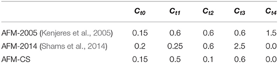
Table 1. Model coefficients for the algebraic turbulent heat flux model.

Validation for Predicting Turbulent Channel Flow at Re_τ=640

Numerical Configuration

In order to assess the solver and numerical configurations employed in this study, it is essential to appropriately define target parameters to show how good the performance of simulation is. In this study, mean velocity, mean temperature, temperature variance, and turbulent heat flux are chosen to prove the accuracy of predicting turbulent properties. Hence, direct numerical simulation (DNS) results of turbulent channel flow at low-Prandtl number fluid published by Abe et al. (2004) are selected in this study for validation purposes. The data found in the literature will be compared with simulation results, and a good agreement will demonstrate the capability of the employed CFD approach.

The computational domain with a size of L_x × L_y × L_z = 6.4δ × 2δ × 2δ has been discretized into N_x × N_y × N_z = 256 × 256 × 128 grid cells based on sensitivity analysis of the grid resolution and geometry size. A schematic sketch of the simulation domain is shown in Figure 1. The related dimensionless numbers for the validation calculations can be found in Table 2. A no-slip velocity condition is imposed on the walls, and the values of turbulent properties on the walls are set to a constant, small value.

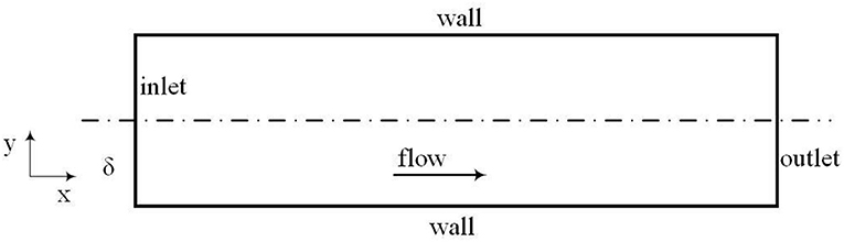
Figure 1. Schematic diagram of the simulation domain.

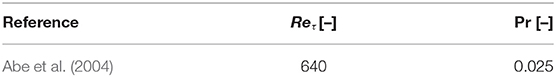
Table 2. Dimensionless numbers for validating the CFD approach employed.

Validation Calculation of the CFD Approach Employed With DNS Results

The predicted results of turbulent channel flow at low Prandtl number are compared with the DNS results from Abe et al. (2004), in which the Reynolds number calculated by the friction velocity is equal to 640. The results employed include the velocity distribution in the near-wall region, temperature profile, temperature variance, and turbulent heat flux in the streamwise and transverse directions. In Figure 2, the simulation results of velocity and temperature distributions are plotted against DNS results. It is clearly indicated that the predicted results show a good qualitative and quantitative agreement with DNS results. The predicted velocity also shows a good agreement with the wall function, while the predicted temperature in the laminar sub-layer is consistent with the function Θ⁺ = y⁺Pr.

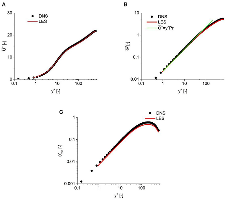
Figure 2. Comparison against the results of Abe et al. (2004). (A) Mean velocity, (B) Mean temperature, and (C) Root mean square of temperature variance.

In order to further validate the simulation results for the prediction of the turbulent heat flux, the predicted temperature variance is plotted against DNS results in Figure 2. It can be observed that a good agreement is also achieved. For the turbulent heat flux, as shown in Figure 3, a good agreement demonstrates the capability of the solver and numerical configurations employed to predict the turbulent and heat transfer properties for low-Prandtl number fluid.

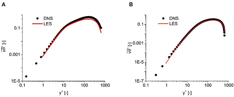
Figure 3. Time-averaged turbulent heat flux compared with the results of Abe et al. (2004). (A) Streamwise direction and (B) Wall-normal direction.

The comparison between the simulation results and the DNS results provided by Abe et al. (2004) demonstrates the capability of the CFD method employed to predict the flow and heat transfer properties in a low-Prandtl fluid. Hence, this numerical configuration will be employed in the following simulation to provide detailed results for turbulent heat flux under a typical flow condition of SFRs.

LES Simulations of Turbulent Channel Flow at Pr = 0.005

Based on the previous study, the LES method is employed in this paper to investigate the time-averaged properties of turbulent statistics and heat flux in sodium flow. The numerical configuration is the same as the validation calculations, as described in section Algebraic Turbulent Heat Flux Model. In the design of the fuel assembly of an SFR, cylindrical fuel rods are arranged in a triangular array. The geometry of the sub-channel formed between walls of fuel rods is quite different from the rectangular channel employed in the validation calculations. In order to eliminate the influence from the geometry, a rectangular channel is still considered in the following simulation with the same range of Reynolds numbers for the SFR. Considering the typical flow rate of a China Experimental Fast Reactor (CEFR), the Reynolds numbers evaluated based on the equivalent diameters of central, side, and corner sub-channels are 25,200, 32,500, and 24,300, respectively. Hence, the Reynolds numbers considered in the current study are chosen from 20000 to 35000, which are calculated by the half-width of the channel and the mean velocity as shown in Table 3. Information on the geometrical size and mass flow rate of the fuel assembly can be found in Chai et al. (2020). It was also the best compromise we could provide due to a limitation of computational resources. Its influence on both turbulent statistics and heat flux will be discussed later. The typical Prandtl number of sodium is also considered in the current study.

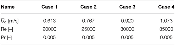
Table 3. Summary of averaged velocity with the corresponding dimensionless numbers.

In order to consider the influence of grid resolution, three different meshes are evaluated in which the total grid number is varied from 3.5 to 8 million, as listed in Table 4. The computational domain employed in this part of the LES simulations is the same as in the previous validation calculations. The finest mesh was discretized into N_x × N_y × N_z = 256 × 256 × 128 grid cells, which is the same as in the previous validation calculations. The value of y+ is kept around 0.5 for all cases. It can be found that the predicted friction velocity tends to approach a constant value when the mesh number is larger than 6 million. With consideration of accuracy and computation efforts, the last mesh is chosen in the following analysis. The simulations were carried out on a Dell R730 server with the Intel Xeon E5-2697 v4 @ 2.30 GHZ (2 CPUs). Each simulation requires almost 168 h to obtain time-averaged values of turbulent properties if using the finest mesh.

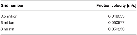
Table 4. Mesh sensitivity analysis.

The instantaneous results of velocity and temperature are shown in Figure 4, in which the Reynolds number is equal to 35,000. Due to a low Prandtl number, small structures can be found in the velocity field, while large structures are more obvious in the temperature field. It is also confirmed that the grids employed to capture the turbulent motions are also sufficient to predict the temperature distribution. Hence, the approximation that the sub-grid heat flux can be neglected in the simulation is justified, as shown in Equation 7.

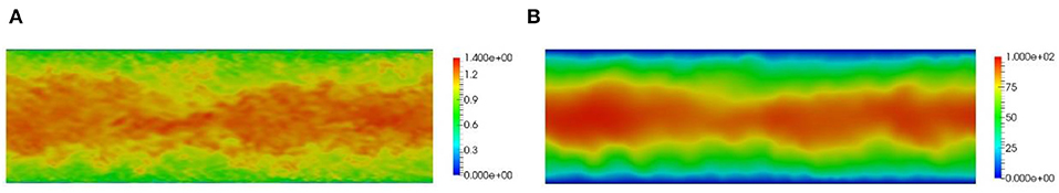
Figure 4. Visualization of simulation results for Re = 35000. (A) Instantaneous velocity and (B) Instantaneous temperature.

In Figure 5, the simulation results of the mean velocity profile in the near-wall region are plotted. The wall function, which includes both the laminar sublayer and the logarithmic region, is also plotted in this figure. It is shown that the predicted results show a good quantitative agreement with theoretical results when the Reynolds number varies.

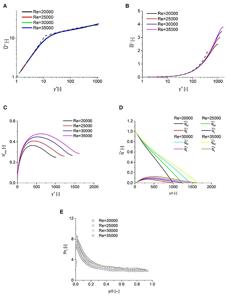
Figure 5. Dependency on Reynolds number. (A) Mean velocity, (B) Mean temperature, (C) Temperature fluctuation, (D) Heat flux decomposition, and (E) Turbulent Prandtl number.

The temperature profiles obtained in the simulation results are shown in Figure 5. It is shown that the linear law, ${\overline{\Theta }}^{+}=y^{+}Pr$, is well-obeyed in the near-wall region for all cases until y⁺ reaches 100. This finding is consistent with the LES results proposed by Duponcheel et al. (2014), in which Prandtl numbers are equal to 0.01. In their results, this dependency tends to vanish when y⁺ reaches 60, which is much smaller than in the current study. It is confirmed that the molecular heat flux is more dominant as the Prandtl number decreases, especially in the near-wall region. Also, the variance of the Reynolds number has little effect on the temperature profile in the laminar sub-layer.

The profiles of temperature fluctuations are also shown in Figure 5. As the Reynolds number increases, the peak of temperature fluctuation is pushed further away from the wall, and their profiles are much flatter than the velocity fluctuation profiles. As the Reynolds number varies from 20000 to 35000, the location of peaks tends to approach the channel center from y⁺ ≈ 400 to y⁺ ≈ 630, which implies an influence of the turbulent motions on the temperature fluctuations. If considering the results of Duponcheel et al. (2014), in which the peaks of temperature fluctuation are at around y⁺ ≈ 500 for two different Prandtl numbers, dependency of temperature fluctuations on the Reynolds number can be identified based on the current study.

As shown in Figure 5, the molecular heat flux is more dominant than turbulent heat flux. Hence, it is necessary to decompose the total heat flux into molecular heat flux and turbulent heat flux and investigate the ratio of these two components. The molecular heat flux is estimated based on the temperature gradient as ${\overline{q}}_M^{+}=P{r}^{-1}d{\overline{\Theta }}^{+}/d{y}^{+}$, while the turbulent heat flux is calculated by ${\overline{q}}_t^{+}=-{\overline{v\theta }}^{+}$. As shown in Figure 5, the molecular heat flux is more dominant and much larger than the turbulent heat flux. As the Reynolds number increases, the peaks of the turbulent heat flux tend to approach the channel center and their values become larger. Furthermore, the results of Duponcheel et al. (2014) suggested that the turbulent heat flux is of the same order or larger than the molecular heat flux. This discrepancy confirms that, for low-Prandtl fluid like sodium, the contribution from the turbulent flux becomes less important, and more attention should be paid to the modeling of the heat transfer process in sodium.

In RANS simulation, the turbulent Prandtl number is used to estimate the ratio between turbulent viscosity and turbulent diffusivity, and its modeling is important for estimating the turbulent heat transfer process, especially for low-Prandtl fluid. The profiles of the turbulent Prandtl number Reynolds number varies are shown in Figure 5. Its value is calculated by turbulent diffusivity and turbulent viscosity as $P{r}_t=\frac{{\nu }_t}{{\alpha }_t}$. The turbulent diffusivity and turbulent viscosity are calculated as ${\alpha }_t=\overline{v^{\prime }{\Theta }^{\prime }}/\frac{d\overline{\Theta }}{dy}$ and ${\nu }_t=\overline{u^{\prime }{v}^{\prime }}/\frac{d\overline{u}}{dy}$, respectively. From the results obtained, it is found that the peaks of the turbulent Prandtl number exist in the near-wall region, followed by a sharp decrease. When approaching the channel center, the turbulent Prandtl number shows a slight decrease. The turbulent Prandtl number profile is consistent with the results of Duponcheel et al. (2014). However, the results obtained in the current study prove that a smaller turbulent Prandtl number can be expected for sodium, the Pr of which is extremely low. Moreover, as the Reynolds number increases, a smaller turbulent Prandtl number can be expected.

Heat transfer performance is usually characterized by the Nusselt number Nu, which is calculated based on the bulk temperature T_b. For liquid metal, several correlations are proposed to estimate the relationship between the Nusselt number and the Peclet number Pe. The Nusselt number obtained from the predicted results was plotted against the Peclet number and compared with the Lubarsky and Kaufman model (Lubarsky and Kaufman, 1955) and the Cheng and Tak model (Cheng and Tak, 2006b), and shown in Figure 6. It can be observed that the latter provides a better prediction accuracy when compared with the LES results, while the Lubarsky and Kaufman model obviously underestimates it.

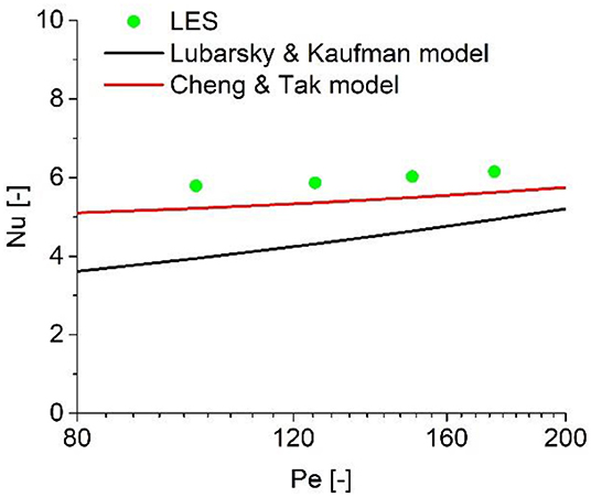
Figure 6. Nusselt number as a function of Peclet number.

RANS Simulations at Pr = 0.005

Because it is numerically economical and robust, the RANS model is a very popular model for investigating the flow and heat transfer properties in a fuel assembly. In this section, the RANS method is employed to investigate the flow and heat transfer properties of turbulent channel flow. All the numerical configuration and boundary conditions are the same as in the LES simulation described in section LES Simulations of Turbulent Channel Flow at Pr = 0.005. The inlet velocity and the corresponding dimensionless numbers can be found in Table 3, which covers the typical range of Reynolds numbers of SFRs. The simulation results obtained in section LES Simulations of Turbulent Channel Flow at Pr = 0.005 are employed to calibrate the parameters used in the algebraic turbulent heat flux model (AFM), which is derived from the full second moment transport equation for the turbulent heat flux under the hypothesis of local equilibrium between production and dissipation (Dol et al., 1997). The optimized coefficients will show more accurate prediction of turbulent heat flux for sodium.

The RANS model is employed to predict the flow and heat transfer properties in a turbulent channel for Pr = 0.005. The range of Reynolds number is consistent with the previous LES simulation. The results provided by AFM-2005 and AFM-2014 are also included in this figure. In this part, a low-Reynolds k-ω SST model is used to evaluate the turbulent viscosity. The predicted velocity profiles show a good agreement with LES results, and hence they are not shown in the following analysis. The predicted temperature profiles are compared with LES results in Figure 7. It is clearly indicated that the existing models, especially AFM-2014, underestimate the variance of coolant temperature in the wall-normal direction. The optimized coefficients show better performance compared with the models found in the literature. This phenomenon can be attributed to the fact that the turbulent heat flux in liquid sodium is greatly reduced due to the extremely low Prandtl number, and the decreased coefficients used in the proposed model are more suitable for reproducing the distribution of turbulent flux.

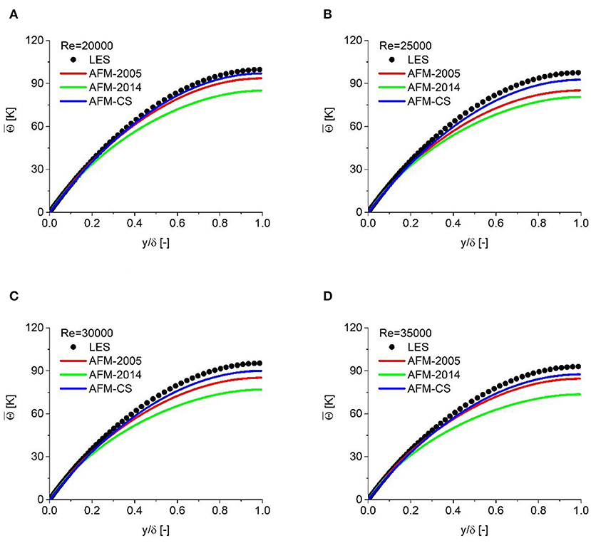
Figure 7. Coolant temperature vs. vertical position for different Reynolds numbers. (A) Re = 20000, (B) Re = 25000, (C) Re = 30000, and (D) Re = 35000.

In order to further assess the calibrated coefficients, the distribution of turbulent heat flux in the wall-normal direction is shown in Figure 8. The profile of turbulent heat flux is quite similar to the previous results for coolant temperature. In comparison with the two models found in the literature, the calibrated model also shows a better prediction accuracy. The predicted results also confirm the fact that these two existing models overestimate the turbulent heat flux, especially AFM-2014. The proposed model, in which smaller coefficients are employed, shows a significant improvement when compared with the LES results. It can be concluded that the optimized coefficients, which are smaller than those in the existing models, show a better prediction accuracy for turbulent heat flux due to the weaker turbulent heat properties caused by the extremely low Prandtl number.

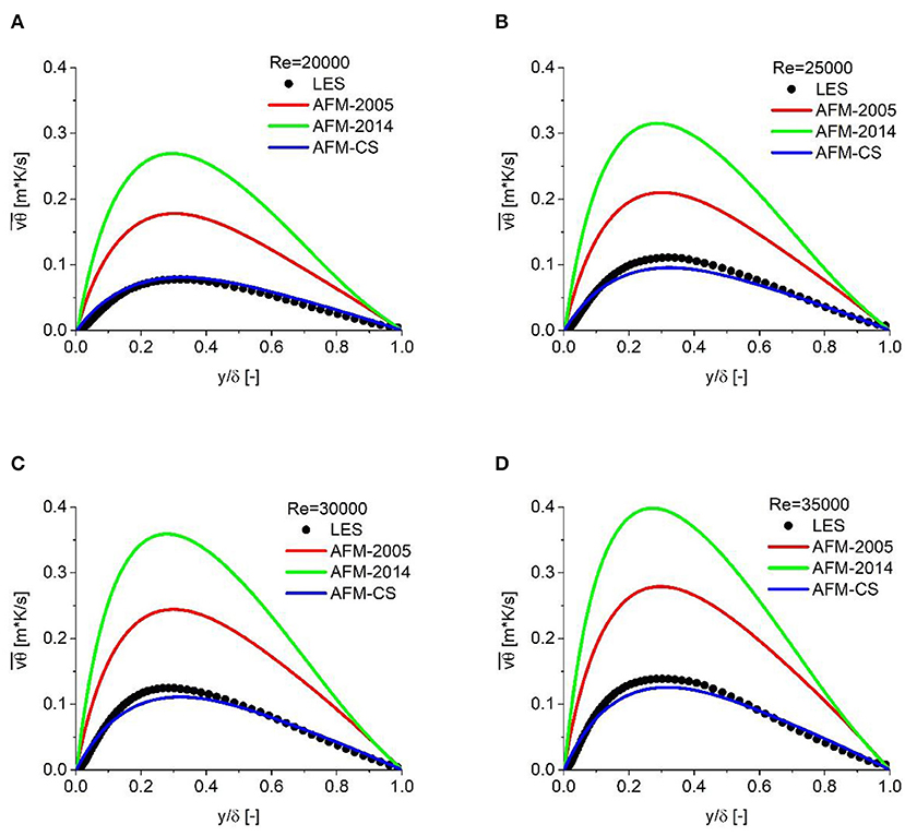
Figure 8. Turbulent heat flux in the wall-normal direction for different Reynolds numbers. (A) Re = 20000, (B) Re = 25000, (C) Re = 30000, and (D) Re = 35000.

Conclusion

In this paper, a numerical method is used to investigate the turbulent heat transfer properties in a turbulent channel flow. A systematic CFD simulation covering the typical range of Reynolds numbers for SFRs was performed at very low Prandtl number: Pr = 0.005, which corresponds to liquid sodium. Based on a wall-resolved LES method, new reference results were obtained for the typical Prandtl number and wall heat flux of an SFR. To prove the correctness of the calculated turbulent and heat transfer properties in low-Prandtl fluid, this method has been compared against DNS results. Statistics of the temperature profile were obtained based on a time-averaged process as well as turbulent heat transfer properties. Based on this configuration, the influence of the extremely low Prandtl number is identified. It is observed that for the channel flow, the peaks of the turbulent Prandtl number exist in the near-wall region, and its value shows a slight decrease while approaching the channel center. Moreover, the results obtained in the current study indicate that, as the Reynolds number increases, a smaller turbulent Prandtl number can be expected. Based on the reference results obtained, the coefficients employed in the algebraic turbulent heat flux model are calibrated. The optimized coefficients have the potential to provide more accurate prediction of coolant temperature for sodium flow as well as turbulent heat flux.

Data Availability Statement

The raw data supporting the conclusions of this article will be made available by the authors without undue reservation.

Author Contributions

XCha carried out the CFD simulation and prepared the manuscript. XL, JX, and XChe provided their suggestion on the contents of the manuscript.

Funding

The work in this paper was supported by the Natural Science Foundation of Shanghai (Grant number: 17ZR1415300) and the National Natural Science Foundation of China (Grant numbers: 11922505 and 51806139).

Conflict of Interest

The authors declare that the research was conducted in the absence of any commercial or financial relationships that could be construed as a potential conflict of interest.

References

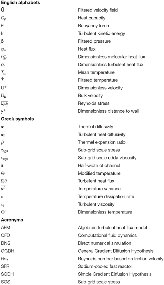
Nomenclature

References

Abe, H., Kawamura, H., and Matsuo, Y. (2004). Surface heat-flux fluctuations in a turbulent channel flow up to Reτ= 1020 with Pr= 0.025 and 0.71. Int. J. Heat Fluid Flow. 25, 404–419. doi: 10.1016/j.ijheatfluidflow.2004.02.010
Bogoslovskaya, G. P., Zhukov, A. V., and Sorokin, A. P. (2000). Models and Characteristics of Interchannel Exchange in Pin Bundles Cooled by Liquid Metal (No. IAEA-TECDOC–1157). International Atomic Energy Agency (IAEA), Vienna.
Chai, X., Zhao, L., Hu, W., Yang, Y., Liu, X., Xiong, J., et al. (2020). Numerical investigation of flow blockage accident in SFR fuel assembly. Nucl. Eng. Design 359:110437. doi: 10.1016/j.nucengdes.2019.110437
Cheng, X., and Tak, N.-I. (2006b). Investigation on turbulent heat transfer to lead–bismuth eutectic flows in circular tubes for nuclear applications. Nucl. Eng. Design 236, 385–393. doi: 10.1016/j.nucengdes.2005.09.006
Cheng, X., and Tak, N. I. (2006a). CFD analysis of thermal-hydraulic behavior of heavy liquid metals in sub-channels. Nucl. Eng. Design 236, 1874–1885. doi: 10.1016/j.nucengdes.2006.02.001
Churchill, S. W. (2002). A reinterpretation of the turbulent Prandtl number. Indust. Eng. Chem. Res. 41, 6393–6401. doi: 10.1021/ie011021k
Da Vià, R., and Manservisi, S. (2019). Numerical simulation of forced and mixed convection turbulent liquid sodium flow over a vertical backward facing step with a four parameter turbulence model. Int. J. Heat Mass Transf. 135, 591–603. doi: 10.1016/j.ijheatmasstransfer.2019.01.129
Dol, H., Hanjalić, K., and Kenjereš, S. (1997). A comparative assessment of the second-moment differential and algebraic models in turbulent natural convection. Int. J. Heat Fluid flow 18, 4–14. doi: 10.1016/S0142-727X(96)00149-X
Duponcheel, M., Bricteux, L., Manconi, M., Winckelmans, G., and Bartosiewicz, Y. (2014). Assessment of RANS and improved near-wall modeling for forced convection at low Prandtl numbers based on LES up to Reτ= 2000. Int. J. Heat Mass Transf. 75, 470–482. doi: 10.1016/j.ijheatmasstransfer.2014.03.080
Grotzbach, G. (2013). Challenges in low-Prandtl number heat transfer simulation and modelling. Nucl. Eng. Design 264, 41–55. doi: 10.1016/j.nucengdes.2012.09.039
Kays, W. M. (1994). Turbulent Prandtl number. Where are we? ASME Transac. J. Heat Transf. 116, 284–295. doi: 10.1115/1.2911398
Kenjeres, S., Gunarjo, S. B., and Hanjalic, K. (2005). Contribution to elliptic relaxation modelling of turbulent natural and mixed convection. Int. J. Heat Fluid Flow 26, 569–586. doi: 10.1016/j.ijheatfluidflow.2005.03.007
Kenjereš, S., and Hanjalić, K. (2000). Convective rolls and heat transfer in finite-length Rayleigh-Bénard convection: a two-dimensional numerical study. Phys. Rev. E 62:7987. doi: 10.1103/PhysRevE.62.7987
Lorenz, J., and Ginberg, T. (1977). Coolant mixing and subchannel velocities in an LMFBR fuel assembly. Nucl. Eng. Design 40, 315–326. doi: 10.1016/0029-5493(77)90042-5
Lubarsky, B., and Kaufman, S. J. (1955). Review of Experimental Investigations of Liquid-Metal Heat Transfer. University of North Texas.
Menter, F. R., Kuntz, M., and Langtry, R. B. (2003). “Ten years of industrial experience with the SST turbulence model,” in 4th International Symposium on Turbulence, Heat and Mass Transfer, ICHMT 4 (Antalya).
Nicoud, F., and Ducros, F. (1999). Subgrid-scale stress modelling based on the square of the velocity gradient tensor. Flow Turbul. Combust. 62, 183–200. doi: 10.1023/A:1009995426001
Pacio, J., Daubner, M., Fellmoser, F., and Wetzel, T. H. (2016). Experimental study of heavy-liquid metal (LBE) flow and heat transfer along a hexagonal 19-rod bundle with wire spacers. Nucl. Eng. Design 301, 111–127. doi: 10.1016/j.nucengdes.2016.03.003
Schumm, T., Frohnapfel, B., and Marocco, L. (2016). Numerical simulation of the turbulent convective buoyant flow of sodium over a backward-facing step. J. Phys. Conf. Ser. 745:032051. doi: 10.1088/1742-6596/745/3/032051
Shams, A., Roelofs, F., Baglietto, E., Lardeau, S., and Kenjeres, S. (2014). Assessment and calibration of an algebraic turbulent heat flux model for low-Prandtl fluids. Int. J. Heat Mass Transf. 79, 589–601. doi: 10.1016/j.ijheatmasstransfer.2014.08.018
Smagorinsky, J. (1963). General circulation experiments with the primitive equations: I. The basic experiment. Monthly Weather Rev. 91, 99–164.
Sun, K. (2012). Analysis of Advanced Sodium-Cooled Fast Reactor Core Designs With Improved Safety Characteristics. Lausanne: École Polytechnique.
Xiong, J., and Cheng, X. (2014). Turbulence modelling for supercritical pressure heat transfer in upward tube flow. Nucl. Eng. Design 270, 249–258. doi: 10.1016/j.nucengdes.2014.01.014