Identification of the Optimum Rain Gauge Network Density for Hydrological Modelling Based on Radar Rainfall Analysis

Abstract

Rain gauges continue to be sources of rainfall data despite progress made in precipitation measurements using radar and satellite technology. There has been some work done on assessing the optimum rain gauge network density required for hydrological modelling, but without consensus. This paper contributes to the identification of the optimum rain gauge network density, using scaling laws and bias-corrected 1 km × 1 km grid radar rainfall records, covering an area of 28,371 km² that hosts 315 rain gauges in south-east Queensland, Australia. Varying numbers of radar pixels (rain gauges) were repeatedly sampled using a unique stratified sampling technique. For each set of rainfall sampled data, a two-dimensional correlogram was developed from the normal scores obtained through quantile-quantile transformation for ordinary kriging which is a stochastic interpolation. Leave-one-out cross validation was carried out, and the simulated quantiles were evaluated using the performance statistics of root-mean-square-error and mean-absolute-bias, as well as their rates of change. A break in the scaling of the plots of these performance statistics against the number of rain gauges was used to infer the optimum rain gauge network density. The optimum rain gauge network density varied from 14 km²/gauge to 38 km²/gauge, with an average of 25 km²/gauge.

1. Introduction

Rainfall is a key forcing input for hydrological modelling, such as that used in studies on extreme events and climate impact analysis. However, the high spatial variability of rainfall is recognised, and thus data regarding the rainfall distribution in space and time is paramount for meaningful use of the outputs of hydrological models. Ground-based rain gauges have been the source of rainfall measurement for quite a long time, and are generally seen as the “ground truth”. However, the poor gauge network density, as a result of limited resources, accessibility and maintenance [1], is a challenge. This is coupled with the fact that gauges provide information for a small area (e.g., 203 mm in diameter), and extrapolating to the spatial scale of several km² introduces high uncertainty (e.g., [2]). In recent years, gridded radar and satellite products data have been processed to obviate the limitations of the gauges, but these approaches have their challenges, including the spatial scale, which ranges from 1 km² to about 50 km². The systematic bias issues that these products suffer range from sensor limitations to sampling errors and the algorithms for retrieval [3]). Although weather radar captures very well the spatial variability, the intensities suffer uncertainties stemming from factors such as beam blocking, ground clutter and signal attenuation [4]. As such, there is always the need to bias-correct these data sources with reference to the gauged measurements, and thus point rain gauge records and interpolation methods will continue to play a key role in hydrological modelling. This obviously means that the combination of rain gauge records with either radar and/or satellite products will continue to be widely used, except for in regions without radar or satellite data [5].

Gridded rainfall products (satellite, radar, general circulation models (GCMs), regional climate models (RCMs) are normally calibrated and validated using rain gauge data, but the poor network density introduces a high degree of uncertainty [6]. It is not just the density of the rain gauge networks, but their non-uniform (irregular) distribution over the catchments, due to issues of accessibility and topography, among other factors, also contribute to the uncertainty [7], bearing in mind the high temporal and spatial variability [8]. Studies on the effects of rain gauge distribution and density on input rainfall and hydrological modelling have highlighted that the key factor in runoff errors is the errors in the input rainfall [9,10].

There have been numerous studies to identify the optimum rain gauge density, but without a consensus being reached. As summarised in [11], there is great variation in the studied catchment sizes and the rain gauge densities used in the various studies. For example, [12] used 10 gauges in a < 0.05-km² (0.005 km²/gauge) catchment, whereas [10] used 60 gauges in a 6400-km² study area. Most of the studies focused on the effect of changing the number of rain gauges on runoff response, and not necessarily on identifying the optimum rain gauge network density [13]. By reducing the number of rain gauges from seven to 1 in a 0.5° × 0.5° grid box, Mishra [14] observed that the absolute error in daily rainfall measurement was reduced by 49%.

Approaches in the literature that improve the quality of satellite and radar rainfall products include the simple scaling method (e.g., [15]). This method corrects the mean values of the gridded data based on bias factors of the gridded and observed data, calculated at the monthly or daily timescale. This method was slightly modified to improve the variance as well, by introducing a power law correction [16]. A major disadvantage of these methods is their failure to leverage the spatial and temporal patterns in the observed data. Quantile mapping (QM) (e.g., [17]) is another popular method that only corrects the marginal distribution, without regard for the spatial connectivity (spatial structure), or the wet- and dry-spell lengths and the transition probability that describe the temporal sequences. Essentially, it transforms the gridded data in order to preserve the marginal distribution of the observed data [18]. Yang et al. [3] presented a framework that uses a Gaussian weighting (GW) interpolation QM approach, in order to bias-correct the PERSIANN-CCS satellite precipitation product over Chile. Bias-correction methods have been applied to GCMs/RCMs outputs [19,20] as well. These methods are based on the assumption that the observed data provide the population distribution, while it is in actuality only a sample of the population, as demonstrated in this paper.

A framework for generating daily rainfields, based on interpolation of point data [21,22,23,24], is adopted for the analysis in this paper. The daily radar rainfall data is bias-corrected using the observed data, before using a stratified sampling approach to sample a given number of rain gauge locations. A major contribution of the paper is the recognition that the marginal distribution of the observed daily data is just a sample, and the population distribution needs to be identified through a bias-correction procedure. In addition, the spatial structure of the radar rainfield was considered as the best representation, but its marginal distribution for the day was bias-corrected. In essence, it is assumed that radar provides the best spatial structure, and the point rain gauges the true intensities. Given a set of point locations in a catchment, a two-dimensional (2D) correlogram is developed and used in an ordinary kriging stochastic interpolation. Leave-one-out cross validation (LOOCV) is used to estimate the performance statistics for a given set of rain gauge numbers. A break in scaling, identified by plots of the performance statistics and the number of rain gauges, was used to infer the optimum rain gauge network density, which is the main aim of this paper.

2. Study Area and Data

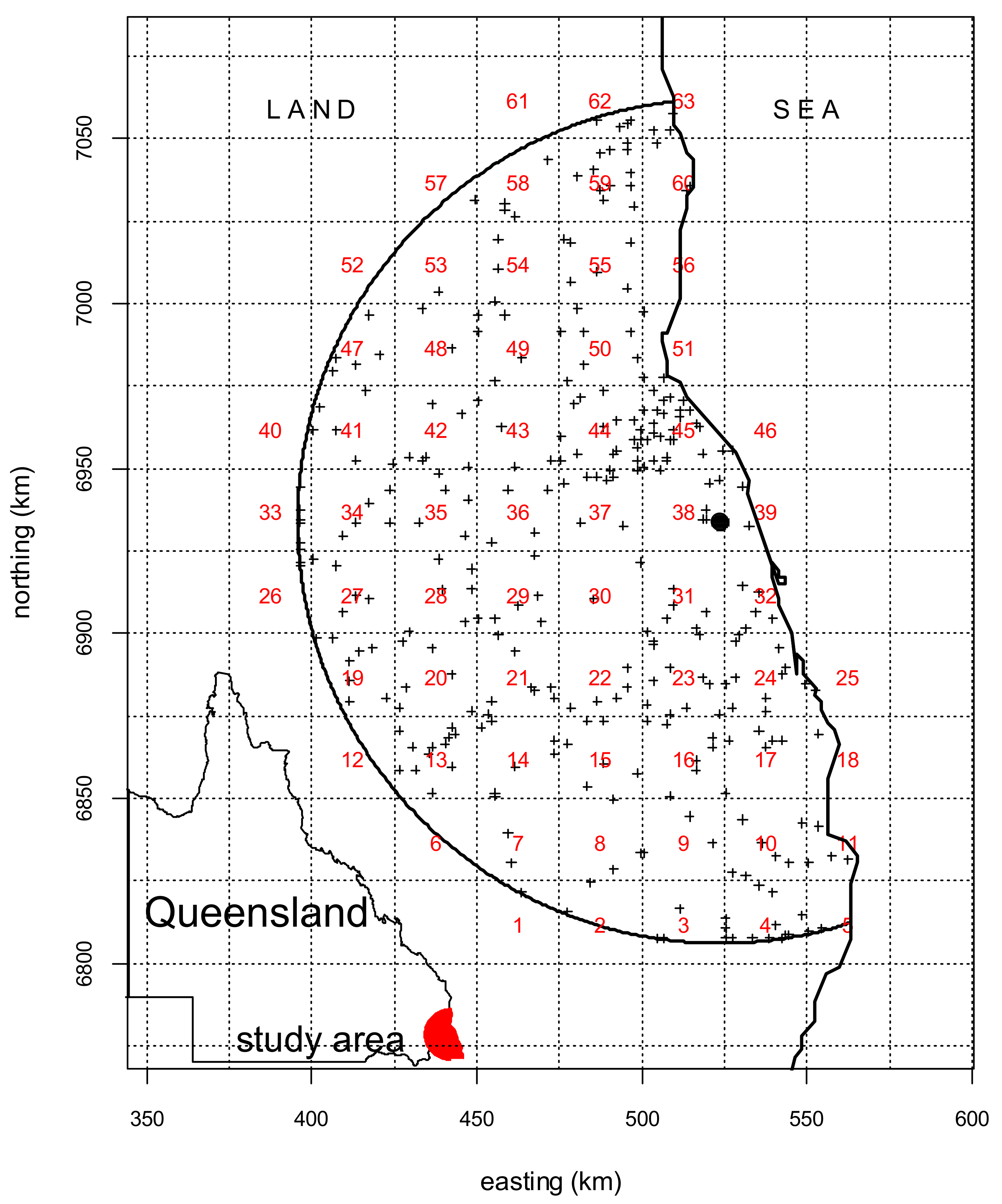
The study area is part of a 128-km radius circular range of the Mt. Stapylton weather radar station, which has a landfall area of 28,371 km² (Figure 1).

It is located in south-east Queensland, and the radar is centred at a latitude of 27.718° S and a longitude of 153.240° E. The radar data has been processed by the Australian Bureau of Meteorology (BOM) (http://www.bom.gov.au/australia/radar/about/calculating_rainfall_accumulations.shtml, accessed on 12 August 2015), and supplied with a 6 min temporal resolution and a spatial unit of 1 km², and from January 1, 2009 to June 30, 2015. However, the radar data were aggregated from 9 a.m. to 9 a.m. in order to conform to the observed daily rainfall sampling timescale. Within the study area, there are 324 rainfall gauges (Figure 1) that are managed by the BOM. Missing records within the daily rainfall data have been infilled by the Queensland Department of Environment and Science (https://www.longpaddock.qld.gov.au/silo/, accessed on 4 April 2020), and the complete records were used. Each rain gauge station is assigned to a 1-km² radar grid centre, and the values of grid centres with more than one rain gauge were averaged, reducing the daily rain gauge stations to 315. The rainfall data from the radar at the 315-gauge locations were extracted to constitute the collocated datasets. This means that for the day of interest, we have the radar (RAD), gauged (GAU) and collocated (COL) datasets for analysis. While the radar data has a minimum wet value of 0.01 mm, the minimum was set to 0.1 mm, to conform with the observed daily rainfall records. It needs to be underlined that partial radar coverage data have been previously used [22,23,24], and this is the first time that the complete landfall area coverage is being used.

A temperate climate, without a dry season and a hot summer, characterises the climate of the study area, in accordance with the classification of [25]. It is a subtropical region, with an average temperature of 26.5 °C, and with summer temperatures sometimes exceeding 29 °C. The region experiences an average annual rainfall of 990 mm, the majority of which occurs during the summer months, from December to March. The winter months from June to August are generally dry, whereas the hot summer months from December to February could experience elevated numbers of thunderstorms.

3. Methodology

3.1. Marginal Distribution Fitting

A standard two-parameter right-skewed distribution is fitted to the daily rainfall amounts greater than zero from the 3 datasets (RAD, GAU and COL) separately. One standard distribution is chosen from the set of Generalized Pareto, Gamma, Gumbel, Log-Logistic, Log-Normal, Kappa and Weibull (R packages fitdistrplus, [26]; FAdist, [27]), using the Anderson-Darling statistic. These right-skewed distributions are considered appropriate for daily rainfall amounts as treated here, and they are commonly used in the literature [28,29,30,31,32]. The fitted distribution is used to transform the daily amounts to probabilities, and then to the standard Gaussian (N [0,1]) quantiles (Q-Q transformation) used in the ordinary kriging interpolation. However, there is a need to account for the dry gauges (zeros) that abound in daily rainfall records. Daily rainfall amounts r at a dry station k with spatial coordinates S_k are assigned as:

$$r\left[s_k\right]\hspace{1em}=\hspace{1em}0.1\exp \left(-\frac{d\left[s_k\right]}{\overline{d}}\right)$$

(1)

where d[s_k] is the minimum distance of the dry gauge located at S_k from a wet gauge, $\overline{d}$ is the average of d, and 0.1 is the minimum wet gauge value. Assuming p_o represents the proportion of the gauges that are dry, the fitted two-parameter distribution F_R is zero inflated and used to transform the rainfall amounts r[s_k] into standard Gaussian quantiles (normal score) w[s_k], as:

$$w\left[s_k\right]\hspace{1em}=\hspace{1em}\begin{array}{c}{\Phi }^{-1}\left[F_R\left(r\left[s_k\right]\right)\left(1-p_0\right)+p_0\right]\hspace{1em}, \hspace{1em}r\left[s_k\right]\ge 0.1\hspace{1em}\\ {\Phi }^{-1}\left[p_0.\exp \left(-\frac{d\left[s_k\right]}{\overline{d}}\right)\right]\hspace{1em}\hspace{1em}\hspace{1em}, \hspace{1em}r\left[s_k\right]<0.1\end{array}$$

(2)

In Equation (2), the cumulative normal distribution N [0,1] is represented as $\mathrm{\Phi }$, and ${\mathrm{\Phi }}^{-1}$ is the inverse. Given a normal score, the inverse of Equation (2), written as

$$r\left[s_k\right]\hspace{1em}=\hspace{1em}\begin{array}{c}{F}_R^{-1}\left[\left\{\mathrm{\Phi }\left(w\left[s_k\right]\right)-p_0\right\}/\left(1-p_0\right)\right]\hspace{1em}, \hspace{1em}\mathrm{\Phi }\left(w\left[s_k\right]\right)\ge p_0\hspace{1em}\\ \hspace{1em}\hspace{1em}\hspace{1em}\hspace{1em}\hspace{1em}0\hspace{1em}\hspace{1em}\hspace{1em}\hspace{1em} \hspace{1em}\hspace{1em}\hspace{1em}\hspace{1em}\hspace{1em}\hspace{1em}, \hspace{1em}\mathrm{\Phi }\left(w\left[s_k\right]\right)<p_0\hspace{1em}\hspace{1em}\end{array}$$

(3)

gives the rainfall amount.

3.2. Bias Correction

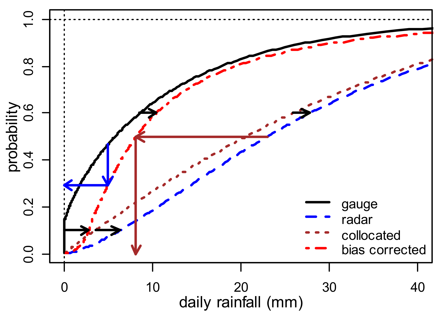
There could be significant differences between the marginal distributions of GAU, RAD and COL datasets for the same day. Hence a bias correction method was implemented. The traditional Quantile-Quantile (Q-Q) bias-correction method assumes that the observed gauge data provide the right distribution, and that the gridded datasets from radar, satellite or GCMs/RCMs therefore need to be adjusted to reflect the observed distribution. This idea is expressed mathematically as (e.g., [18])

$$R_{RAD-BC}\hspace{1em}=\hspace{1em}{F}_{GAU}^{-1}\left[F_{RAD}\left(R_{RAD}\right)\right]$$

(4)

and is used to correct the gridded radar rainfall amounts (R_RAD) to bias-corrected (R_RAD−BC) amounts, using the rain gauge data distribution (F_GAU) and radar data distribution (F_RAD) for the day, F⁻¹ being the inverse function. However, the observed daily records as used in this paper are seen as a sample, and therefore require adjustment as well. As presented later, the number of rain gauges is not high enough to reproduce the spatial structure for a wet day.

For a given probability p, the fitted distributions (F_GAU, F_RAD, F_COL) are used to estimate the rainfall amount for GAU, RAD and COL. Then, the difference between the RAD and COL amounts is added to the GAU in order to obtain amounts that follow the “true” distribution (F_TRUE) of daily rainfall (R) for the day. This is expressed mathematically as:

$$R(p)\hspace{1em}=\hspace{1em}{F}_{{}_{TRUE}}^{-1}(p)\hspace{1em}=\hspace{1em}{F}_{GAU}^{-1}(p)\hspace{0.33em} + \hspace{0.33em}{F}_{RAD}^{-1}(p)\hspace{0.33em} -\hspace{0.33em}{F}_{COL}^{-1}(p)$$

(5)

Given the GAU rainfall amounts (R_GAU), the true distribution is then used to estimate the bias-corrected probabilities ($p_{GAU-BC}$), whereas, for the RAD, the probabilities [F_RAD(R_RAD)] are used to adjust the rainfall amounts, as:

$$\begin{array}{l}{p}_{GAU-BC}\hspace{1em}=\hspace{1em}{F}_{TRUE}(R_{GAU})\\ R_{RAD-BC}\hspace{1em}=\hspace{1em}{F}_{TRUE}^{-1}\left[F_{RAD}(R_{RAD})\right]\end{array}$$

(6)

Therefore, the observed rainfall amounts are preserved, but their probabilities are reassigned, whereas the reverse is the case for the radar rainfall. Figure 2 illustrates the bias-correction scheme. Hereafter, the bias-corrected radar daily rainfall amounts are used.

3.3. Spatial Structure Modelling

The spatial structure required by the ordinary kriging interpolation is developed using the standard Gaussian quantiles, due to the normality assumption of kriging. It is based on the framework presented by [33], which uses the ‘round-trip’ fast Fourier transform approach on the empirical correlogram $\tilde{R}\left[i,j\right]$, obtained as:

$$\tilde{R}\left(x,y\right)\hspace{1em}=\hspace{1em}\frac{1}{N_h}{\displaystyle \sum _{k=1}^{N_h}w\left[s_k\right]}w\left[s_k+h\right]-m_0{m}_{+h}\hspace{1em}, \hspace{1em}\forall (s_k,s_k+h):h\in (x\pm 1,y\pm 1)$$

(7)

In Equation (7), x and y are the separation distances, in km, in the eastern and northern directions, respectively, from the origin (0,0) of the empirical correlogram. Pair gauge locations at separation distance h within the bounded region of $\left(x\pm 1,y\pm 1\right)$ are included in the calculation of the correlogram value at the grid point $\left(x,y\right)$, with $N_h$ representing the number of pair gauges. The means of the pair of tail $w\left[s_k\right]$ and head $w\left[s_k+h\right]$ values are denoted as $m_o$ and $m_{+h}$, respectively.

Following [21,22], a 2D exponential distribution expressed as

$$R_{\Theta }\left(x,y\right)=R_{\Theta }\left(u,v\right)\hspace{1em}=\hspace{1em}\exp \left\{-{\left[{\left(\frac{u}{L_u}\right)}^2+{\left(\frac{v}{L_v}\right)}^2\right]}^{1/2}\right\}\hspace{1em}, \hspace{1em}\begin{array}{c}u=y\sin (\theta )+x\cos (\theta )\\ v=y\cos (\theta )-x\sin (\theta )\end{array}$$

(8)

was fitted to the empirical correlogram data. Along an elliptical contour, u and v are the separation distances in the direction of the major and minor axes, respectively. The 3 parameters defining the 2D exponential distribution are the angle between the major axis and the horizontal direction (θ), the major axis length (L_u), and the minor axis length (L_v), the anisotropy ratio (η) being defined as L_v/L_u. These parameters are estimated using the global optimisation technique of [34] by matching the empirical and the analytical elliptical correlogram contours [21].

3.4. Stratified Sampling of Rain Gauge Locations

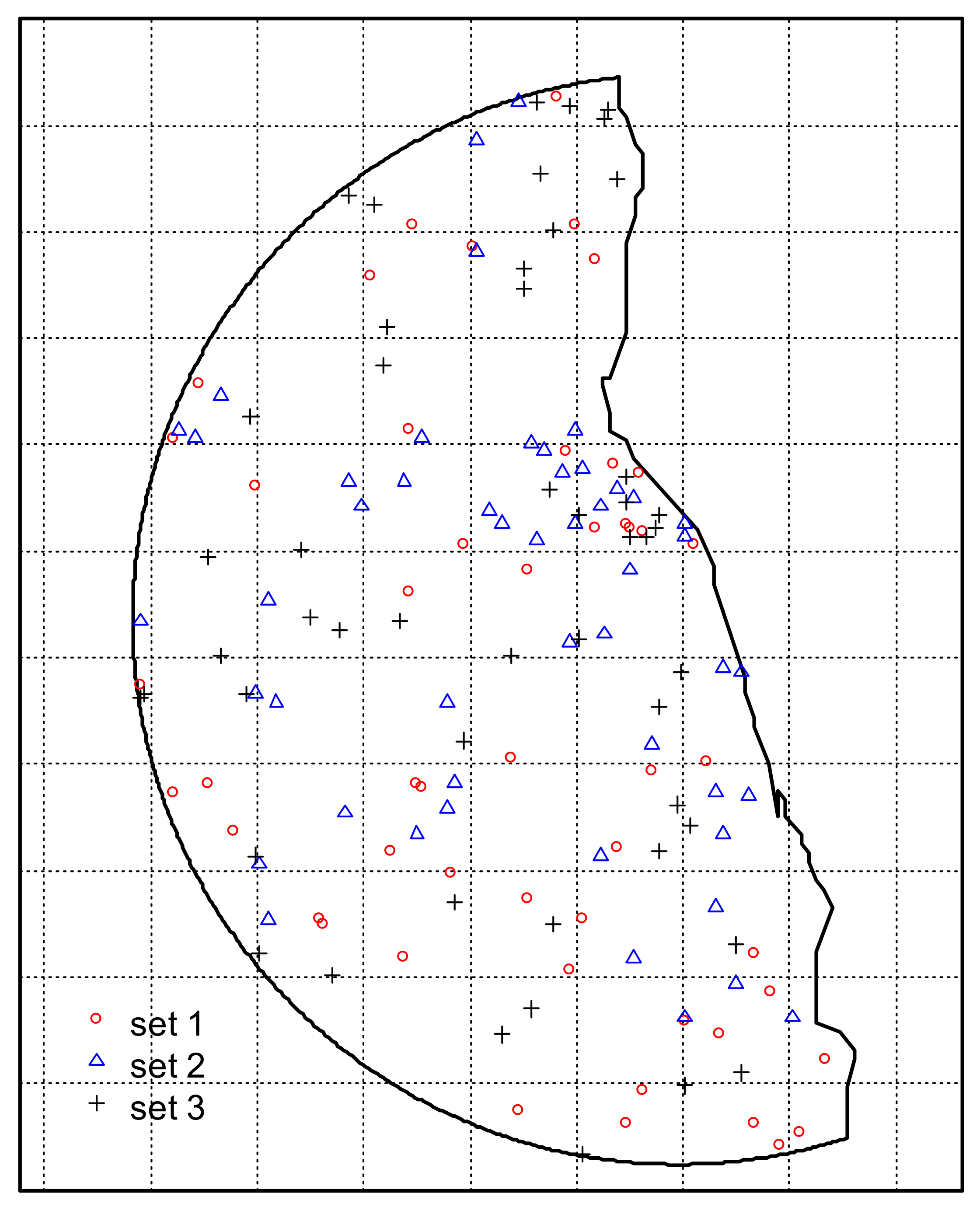
In order to investigate the effects of the number of rain gauges (radar pixels used interchangeably) on the spatial structure, a set number of rain gauges were sampled from the grid centres of the radar data. It is a known fact that rain gauges are by no means uniformly distributed over a study region, as exemplified in Figure 1 for the study region. Therefore, a stratified sampling approach was adopted to mimic the spatial distribution of the current rain gauges. These are the steps for the stratified sampling approach:

• Firstly, the study region was overlaid with a 25 km × 25 km grid, and the resulting 63 blocks within, or intersecting, the study region are labelled in Figure 1;
• Secondly, rain gauges within each grid were counted, and those blocks devoid of gauges were assigned a value of 0.5 times the fraction of the grid within the radar coverage, to allow for possible selection of gauges within the fractional grids, particularly for higher sampling numbers. The rain gauge network density of the grids varies from 1.7 to 48.6 gauges per 1000 km², grid 45 recording the highest density;
• Thirdly, the observed rain gauge counts within the grids were used to develop the weights for the stratified sampling;
• Fourth, the number of rain gauges required were sampled with replacement from integers 1 to 63, representing the grids, in accordance with their weights;
• Finally, the numbers of samples from each grid from the previous step were sampled randomly, without replacement from the subset of the grid, noting that the subset of each grid is the number of 1-km² radar grid centres it contains, which varies from 6 (grid 61) to 625 (the inner grids).

The set of the number of rain gauges sampled from the radar grid centres is {20, 50, 100, 200, 315 (number of observed gauges), 500, 750, 1000, 1250, 1500, 1750, 2000, 3000, 5000, 7500, 10,000, 15,000, 20,000, 28,371 (full radar)}. Because the variability in the spatial structure and the mean distance between gauges is highest for the lowest number of rain gauges, the number of repetitions was varied as {50, 45, 40, 35, 30, 25, 20, 20, 20, 20, 20, 20, 20, 20, 20, 20, 10, 10, 1} for the set of the number of rain gauges, respectively. Figure 3 shows the spatial distribution of 3 sets having a number of rain gauges of 50, which mimics very well the spatial distribution of the observed rain gauges.

3.5. Performance Statistics

Ordinary kriging does not require a description here, as it has been well documented in the literature (e.g., [35,36]). However, it suffices to say that it estimates a variable at a target location using known values at several locations in space, and it is based on linear weighted least squares. For each set of a number of rain gauges sampled, one of the distributions discussed in Section 3.1 was fitted and used to convert the rainfall amounts to standard normal quantiles by means of Equation (2). Then, a 2D correlogram was fitted as explained in Section 3.3. Next, leave-one-out cross validation (LOOCV) was performed using the R package gstat [37]. LOOCV leaves one data point out at a time, and its prediction is made using the remaining data points. The predictions in the normal score were converted to rainfall amounts using Equation (3). The predicted values were evaluated using the root-mean-square-error (RMSE) and the mean-absolute-bias (MAB) performance statistics, defined as:

$$\mathrm{RMSE}\hspace{1em}=\hspace{1em}\sqrt{\frac{1}{N}{\displaystyle \sum _{i=1}^N{\left[V_O(i)\hspace{0.33em}-\hspace{0.33em}{V}_P(i)\right]}^2}}$$

(9)

$$\mathrm{MAB}\hspace{1em}=\hspace{1em}\frac{1}{N}{\displaystyle \sum _{i=1}^N\left|V_O(i)\hspace{0.33em}-\hspace{0.33em}{V}_P(i)\right|}$$

(10)

where the observed and predicted values for the ith gauge are, respectively, V_O(i) and V_P(i), and N is the number of sampled rain gauges. The variation of the performance statistics with the number of rain gauges is used to identify the optimum rain gauge network density.

4. Results and Discussion

A total of 24 wet days, with varying statistical properties, were selected for the analysis (

Table 1. Statistics of the selected radar wet days after bias correction.

Date	MN	SD	WP	MAX	LX	LY	AR	AA
	(mm)	(mm)	(-)	(mm)	(km)	(km)	(-)	(degrees)
20090102	12.2	11.5	0.995	163.8	40.1	23.4	0.583	143.8
20090402	16.8	11.9	0.381	76.2	86.7	50.3	0.581	74.7
20090405	16.0	15.5	0.875	107.4	38.4	23.0	0.600	136.5
20090413	7.3	8.7	0.445	70.1	63.9	28.2	0.442	78.3
20101011	63.1	40.8	0.962	353.7	103.0	59.6	0.579	6.1
20101211	5.8	5.1	0.147	35.7	44.4	17.5	0.395	118.5
20101216	4.6	2.9	0.872	46.8	67.0	47.1	0.703	37.0
20110105	3.9	1.7	0.551	5.9	78.3	68.2	0.870	77.5
20110523	4.9	4.5	0.454	56.5	50.2	42.7	0.851	71.0
20110830	6.4	8.9	0.258	99.9	44.1	22.3	0.505	163.1
20111223	4.1	2.7	0.094	18.3	56.8	45.6	0.804	122.0
20120125	102.2	64.6	1.000	450.1	91.9	59.0	0.642	98.9
20121218	5.6	5.1	0.590	68.4	72.6	64.2	0.885	108.0
20130530	4.0	5.2	0.509	45.6	66.5	64.0	0.962	82.3
20130630	4.0	2.6	0.365	11.0	90.9	55.8	0.614	74.9
20140122	7.4	4.7	0.373	15.0	52.4	49.4	0.943	126.1
20140123	3.1	1.4	1.000	5.1	59.0	31.4	0.533	169.3
20140328	119.7	43.7	1.000	353.2	70.2	60.8	0.866	16.2
20141119	5.3	4.4	0.278	28.7	23.1	17.1	0.739	17.0
20141205	11.2	11.6	0.826	65.2	49.3	35.6	0.722	120.3
20141218	3.6	5.6	0.987	59.5	53.3	27.6	0.517	33.4
20150102	4.2	3.6	0.605	45.4	35.3	23.8	0.674	113.6
20150126	10.6	10.2	0.338	67.0	46.1	30.2	0.656	93.8
20150127	8.8	13.9	0.487	204.6	31.7	22.3	0.703	152.5
Minimum	3.1	1.4	0.094	5.1	23.1	17.1	0.395	6.1
Average	18.1	12.1	0.600	102.2	59.0	40.4	0.682	93.1
Maximum	119.7	64.6	1.000	450.1	103.0	68.2	0.962	169.3

MN—mean rainfall (pixels ≥ 1mm); SD—standard deviation of rainfall (pixels ≥ 1mm); WP—proportion of pixels with rainfall ≥ 1mm; MAX—maximum rainfall; LX—major axis length; LY—minor axis length; AR—anisotropy ratio; AA—anisotropy angle.

).

As seen in Table 1, the mean of pixels that registered rainfall amounts ≥ 1 mm varies between 3.1 mm and 119.7 mm, while the proportion of wet pixels ranges from 0.094 to 1. For the maximum pixel rainfall, the range is from 5.1 mm to 450 mm.

4.1. Marginal Distribution

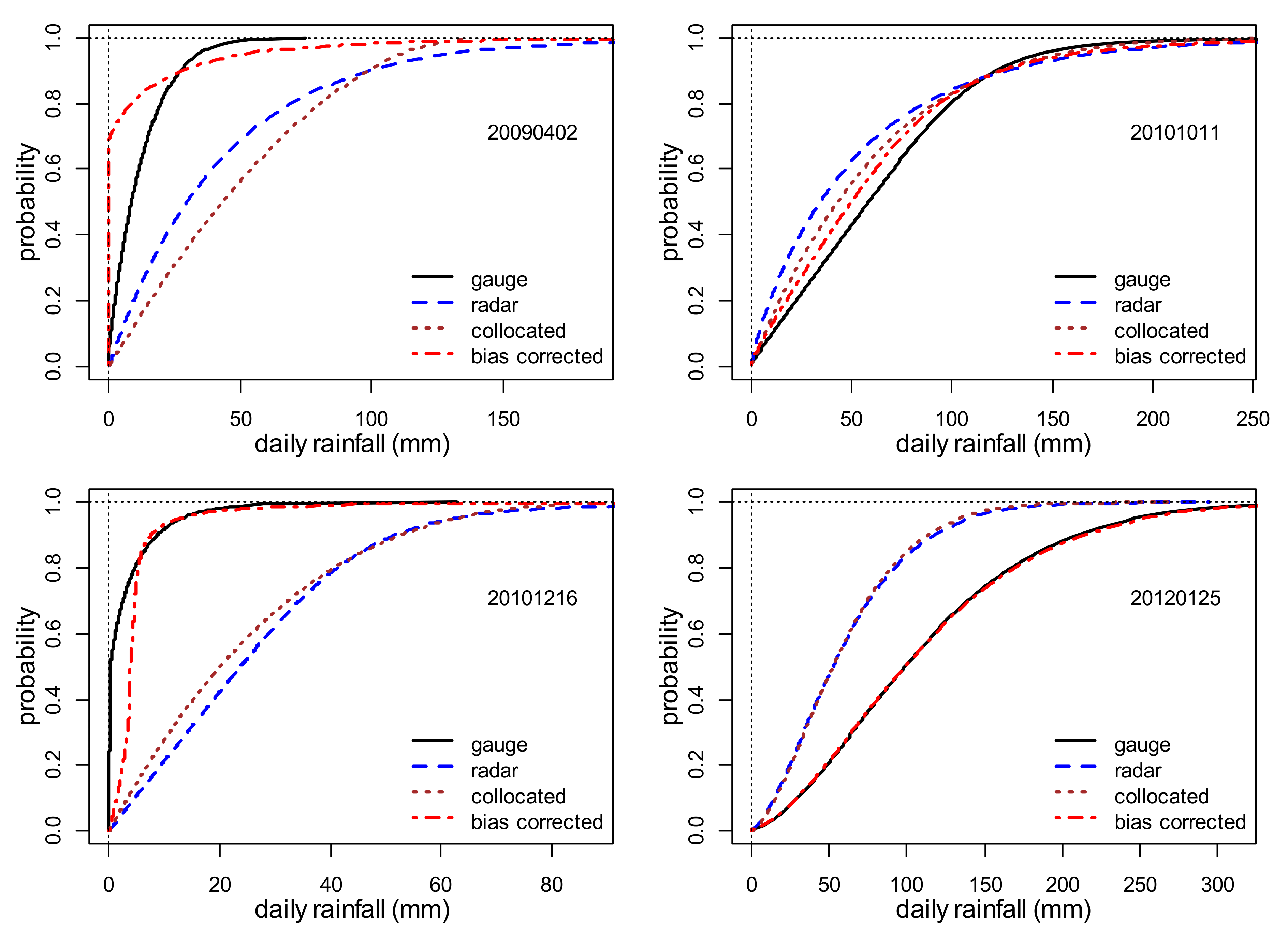
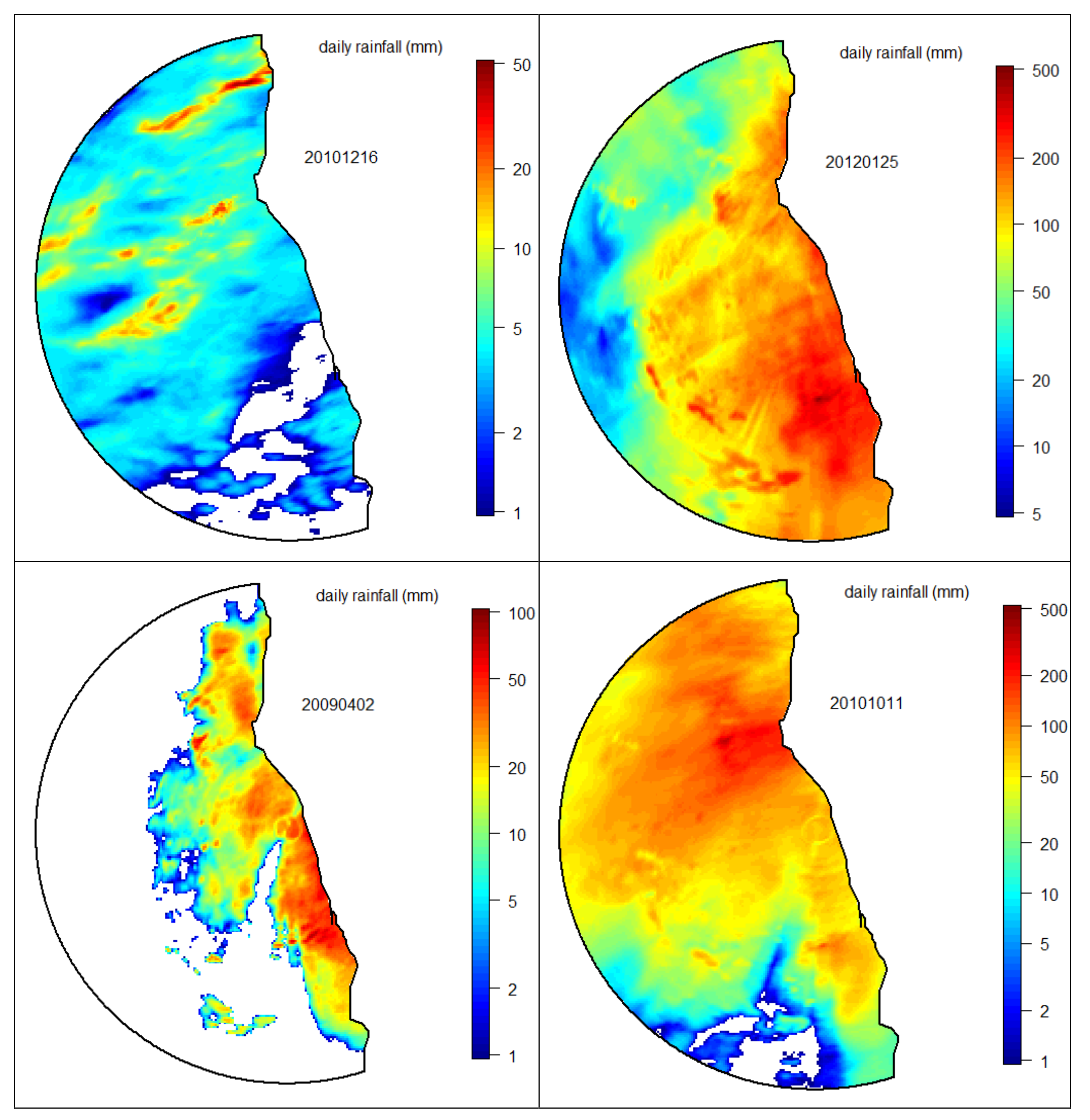
Figure 4 shows the results of the bias-correction scheme applied to the marginal distributions of four selected wet days, and their bias-corrected rainfields are depicted in Figure 5. In many cases, radar overestimates (demonstrated by 20290402, 20101216) or underestimates (demonstrated by 20101011, 20120125) the observed rainfall [38,39], explaining why bias-correction is necessary (e.g., [40]).

Some of the errors stem from the methods used for converting radar reflectivity to rainfall intensity and ground clutter. For day 20120125, the collocated distribution was in sync with that of the full radar, but different from the distribution of the rain gauge data. A such, the agreement between the full radar and the collocated marginal distributions depends on the spatial distribution of rainfall, which varies significantly across the wet days.

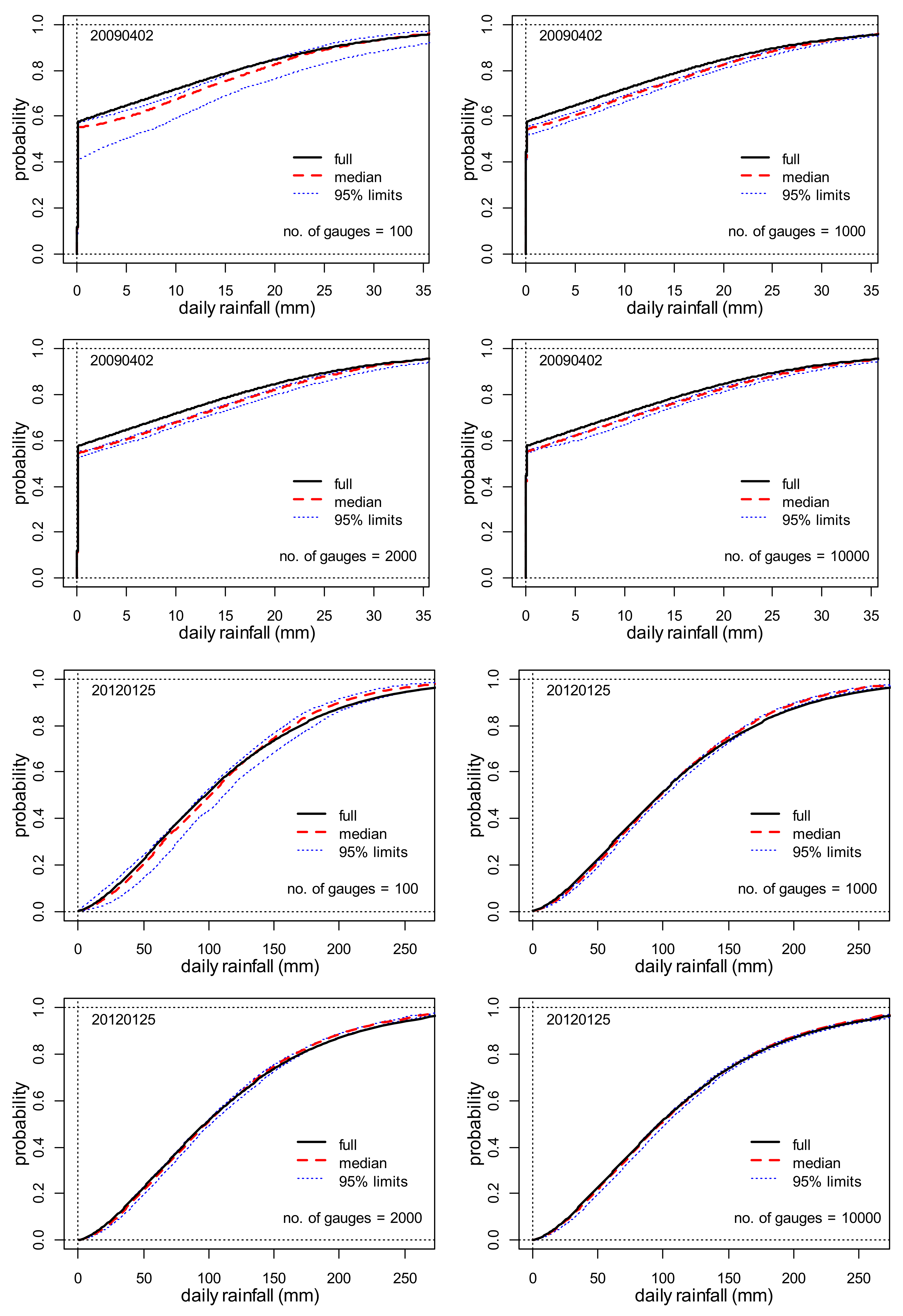
Rainfall amounts were sampled from the bias-corrected radar images corresponding to a given number of rain gauges. This was repeated a number of times, as explained in Section 3.4. An empirical distribution is fitted to each sampled dataset. For a given probability, rainfall amounts from the repeated samples were used to define the median and the 95% prediction limits for that probability. Figure 6 compares the median empirical distribution with the one derived from the full radar. While the median distribution is quite close to the full radar for all numbers of gauges, the widths of the prediction limits decrease with increasing numbers of gauges. Again, the spatial distribution of rainfall for the day will determine how the median distribution of the smaller number of gauges matches the full radar case. As shown in the two examples, the higher the coefficient of variation for the rainfall data, the higher the variability around the median distribution.

4.2. Spatial Structure Parameters

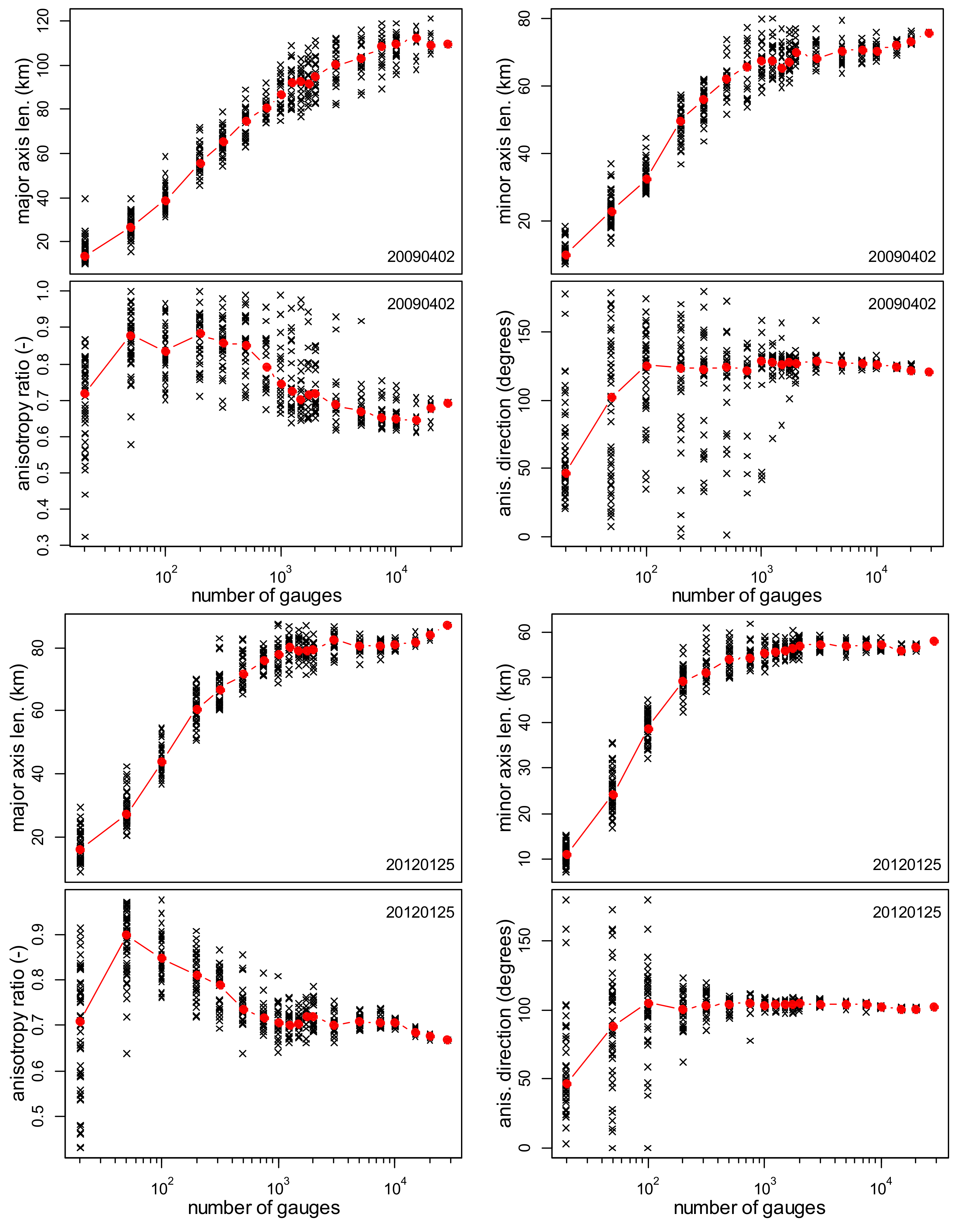
For each set of sampled rainfall data for a fixed number of gauges, Equations (1) and (2) were used to convert rainfall data into normal scores. The Section 3.3 methodology was applied to derive the 2D correlogram parameters of the major and minor axis lengths, as well as the anisotropy direction and ratio. Figure 7 shows the variation of the correlogram parameters with the number of gauges for two wet days. Both the major and minor axis lengths increase similarly as the number of gauges increases, at a rate of over 40% for an additional gauge at 50 gauges, and drops sharply to less than 1% between 1000 and 1500 gauges, using the median values. While there is considerable variation in the anisotropy direction up to about 2000 gauges, the median stabilises quite well after 100 gauges. These observations point to the fact that daily rainfall varies considerably from wet day to wet day, and reflecting the true spatial structure entirely depends on the number and location of the gauges. It needs to be pointed out that the patterns displayed in Figure 7 were also observed by [21] using radar rainfall records from the Bethlehem station in South Africa, but no analyses, as done in this paper, were made.

4.3. The Optimum Rain Gauge Network Density

In this section, each set of sampled rainfall data for a fixed number of gauges is used to develop the marginal distribution and the 2D spatial structure required by the ordinary kriging interpolation. The LOOCV technique was used to simulate rainfall amounts, which were evaluated using RMSE and MAB, as presented in Section 3.5, thus incorporating uncertainties into the marginal distribution and the 2D spatial structure, because of the inadequate number of gauges sampled.

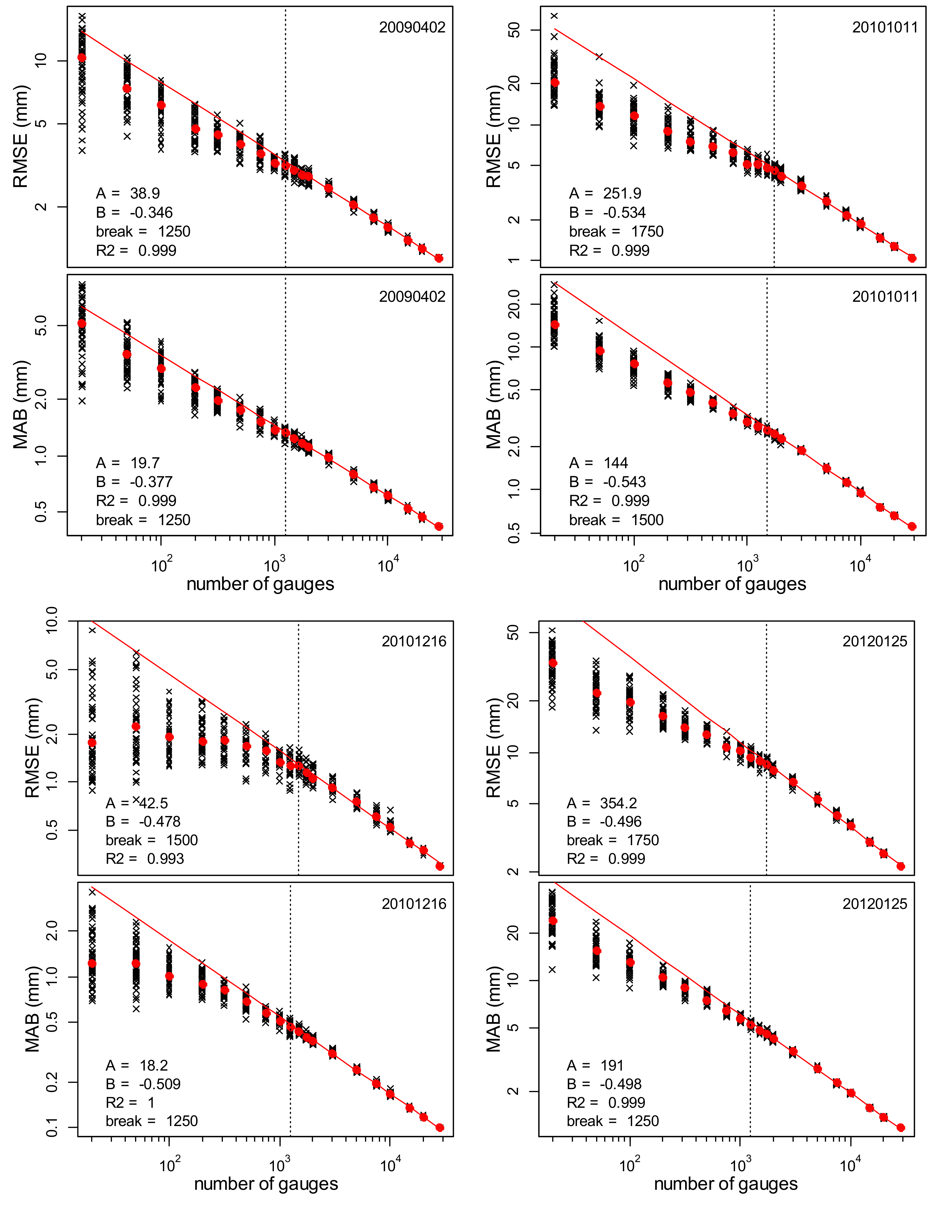
Figure 8 shows plots of the performance statistics (RMSE and MAB) against the number of gauges for the different sampled datasets. The median values of the repeated samples for a fixed number of gauges are shown as solid circles. It is not surprising that the variability of the performance statistics, with regards to the median values, is higher for the smaller number of gauges.

As the rain gauge network density increases, the inter-gauge distances are decreased, thus increasing the correlation between the gauges that results in the observed decreasing performance statistics. After 2000 gauges, there is virtually no variability in the median. Of note is the perfect power law scaling beyond 2000 gauges for all performance statistics, as empirically observed for all wet days. Therefore, a power law of the form

$$PS\hspace{1em}=\hspace{1em}A.N^B$$

(11)

was fitted to the median values after the number of gauges passed 2000. In Equation (11), PS indicates a performance statistic which is either RMSE or MAB, N is the number of gauges, and A and B are the power law coefficient (normalising factor) and scaling exponent, respectively. Gyasi-Agyei et al. [41] used such a power law to relate the channel network average link slope to contributing catchments. They used the break in the scaling exponent (B) to delineate hillslope from the main channel network of a catchment. In the presentation here, the fitted power law line is extended to the lowest number of gauges, in order to determine at which number of gauges there is a break in the scaling, i.e., departure from the scaling law. This breaking point is identified as the optimum number of gauges, and thus there is no appreciable increase in information gained when the number of gauges is increased beyond this point.

In

Table 2. Root-mean-square-error (RMSE) and mean absolute bias (MAB) scaling parameters.

Date	RMSE				MAB			Average
	A	B	Break	A		B	Break	Break
20090102	122.1	−0.456	2000	57.4		−0.494	1500	1750
20090402	38.9	−0.346	1250	19.7		−0.377	1250	1250
20090405	121.2	−0.437	1000	58.8		−0.422	500	750
20090413	54.2	−0.496	2000	16.4		−0.476	1250	1625
20101011	251.9	−0.534	1750	144.0		−0.543	1500	1625
20101211	17.6	−0.380	2000	7.8		−0.420	2000	2000
20101216	42.5	−0.478	1500	18.2		−0.509	1250	1375
20110105	18.6	−0.463	1500	9.1		−0.456	750	1125
20110523	23.3	−0.387	1750	12.0		−0.429	1000	1375
20110830	34.6	−0.390	2000	17.4		−0.456	750	1375
20111223	6.6	−0.327	1500	3.6		−0.378	1250	1375
20120125	354.2	−0.496	1750	191.0		−0.498	1250	1500
20121218	49.9	−0.467	1000	13.7		−0.438	750	875
20130530	20.2	−0.383	750	10.8		−0.416	750	750
20130630	12.8	−0.491	1750	4.6		−0.453	750	1250
20140122	37.2	−0.508	1000	11.3		−0.466	1250	1125
20140123	13.2	−0.495	2000	7.0		−0.496	1250	1625
20140328	325.7	−0.511	2000	153.9		−0.505	1000	1500
20141119	30.5	−0.405	1000	10.2		−0.388	500	750
20141205	135.9	−0.503	2000	43.9		−0.473	750	1375
20141218	48.2	−0.443	1500	20.4		−0.465	1000	1250
20150102	34.9	−0.446	2000	11.9		−0.408	1000	1500
20150126	95.1	−0.479	1000	24.5		−0.436	1750	1375
20150127	70.2	−0.354	750	27.5		−0.388	750	750
Minimum	6.6	−0.534	750	3.6		−0.543	500	750
Average	81.6	−0.445	1531	37.3		−0.450	1073	1302
Maximum	354.2	−0.327	2000	191.0		−0.377	2000	2000

A—scaling constant; B—scaling exponent; break—break in scaling.

, the values of the scaling coefficient and exponent of the fitted power law for the different wet days are shown. It is observed that the scaling exponent of RMSE and MAB are not significantly different for the same day at the 5% level (paired T test p-value = 0.49; F test p-value = 0.2), but the breaking point identified could be significantly different; about 460 on average. With respect to RMSE, the breaking point varies from 750 gauges (38 km²/gauge) to 2000 gauges (14 km²/gauge), while for the MAB it could be as high as 56 km²/gauge for a few wet days. Dwelling on the averages, RMSE yielded 18 km²/gauge and MAB 26 km²/gauge, and their combination yielded 22 km²/gauge. These average values translate to grid sizes of 4 km for RMSE, 5 km for MAB, and 4.7 km for the combination. There is no apparent correlation between the scaling exponents and the listed rainfall properties in Table 1, with the exception of the wet proportion, which exhibits correlation coefficients of −0.6 with RMSE and −0.7 with MAB. This means that as the wet proportion increases, the power law scaling slope becomes steeper.

Another way to estimate the representative threshold values was to use rate of change (ROC), estimated as

$$RO{C}_i\hspace{1em}=\hspace{1em}\frac{P{S}_{i+1}-P{S}_i}{P{S}_i(N_{i+1}-N_i)}100$$

(12)

where i and i+1 are the successive number of gauges indexed when arranged in increasing order, (N_i+1 − N_i) is the difference in the number of gauges, and (PS_i+1 − PS_i) represents the difference in performance statistics at the successive intervals. In comparison to RMSE and MAB, the ROC is rainfall magnitude-independent, meaning values for the different wet days could be compared. Rates of change (ROC) is commonly used in finance to measure the change in the price of a security over a fixed time interval, so the denominator (N_i+1 − N_i) is not required, or set to 1, in that sense (https://www.ambroker.com/en/analysis/blog/what-rate-change-roc-indicator-and-how-use-trading/, accessed on 2 June 2020). The ROC was calculated progressively for all increasing numbers of gauges for each wet day. For a fixed number of gauges, the medians of the 24 values were selected and plotted in Figure 9.

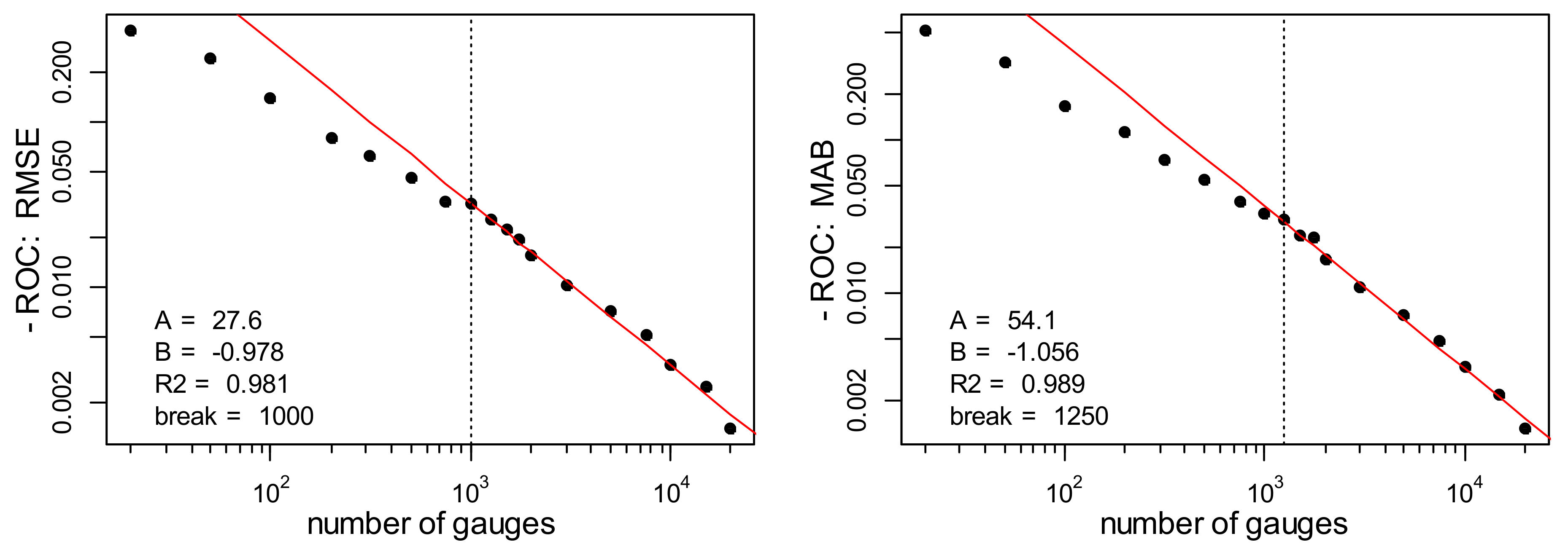
As was done for the individual days of RMSE, demonstrated in Figure 8, the power law curve (Equation (11)) was fitted to the number of gauges beyond 2000, and extrapolated to the lower number of gauges to identify the scaling breaking point. Because both the RMSE and MAB show decreasing trends with increasing numbers of gauges, resulting in negative ROC values, absolute values of ROC (or −ROC) were used to allow the fitting of the power law. Clearly, the breaking point is 1000 for the ROC of the RMSE, and 1250 gauges for that of MAB, the average of both performance statistics being 1125 gauges. These breaking points are slightly lower than the average of the breaking points of individual wet days, as presented in Table 2. A breaking point of 1125 gauges translates to an optimum rain gauge density of 25 km²/gauge, and a grid size of 5 km. Since the current rain gauge density of the case study site is 90 km²/gauge (28,371/315), the implication of our finding is that this density needs to be improved by at least a factor of three, to mimic the full-scale level. Due to economic constraints, this may not be the way to go, and it may be necessary to rely on blending radar and satellite records with whatever gauge network density is affordable, while remaining aware of the need to be wary of the consequences. Hence ground based rain gauges will continue to be widely used and play a significant role in hydrological analysis and modelling.

Girons Lopez et al. [10] used an inverse-distance weighting method to interpolate a varying number of rain gauges over a 6400-km² study area in north-eastern Switzerland. Using a Pearson correlation coefficient and the normalised RMSE (NRMSE), they concluded that increasing the rain gauge network density beyond 24 per 1000 km² (42 km² per gauge, grid size of 6.4 km) did not improve the performance statistics. Their threshold value for the optimum rain gauge density is not significantly different from what has been observed in our case study, our average optimum being a grid size of 5 km. However, a grid size of 4 km (2000 gauges) is ideal for all wet days. Villarini et al. [7] witnessed the power law type decrease in the NRMSE of catchment-wide average rainfall when the numbers of rain gauges were increased, although they did not fit a power-curve to investigate whether there is a breaking point in the scaling behaviour, as this was not their objective. However, they recommended a minimum of four gauges to evaluate satellite pixels of about 200 km² for daily rainfall, and they established a scaling behaviour (power law) between the NRMSE of rainfall accumulation and the sampling interval.

This study has provided one insight into the evaluation of the daily satellite precipitation products that come with different grid sizes. The grid size of 4 km for PERSIANN_CCS [42] and TASAT [43] satellite products may be ideal. Certainly, precipitation satellite products with grid sizes of 10 km or greater may require spatial downscaling to a finer grid size, for better hydrological modelling.

5. Conclusions

The rain gauge continues to be a valuable source of rainfall records, despite its primary limitation of having a small coverage area, of about 203 mm in diameter, and an inadequate network density, rendering it unable to capture the high spatial variability of rainfall. For these reasons, radar and satellite rainfall data sources are becoming popular, but can be cost-prohibitive for some areas. With the aid of bias-corrected radar daily rainfall records, this study has provided a framework for determining the optimum rain gauge density. The probabilities of the radar records are assumed to be correct, but the rainfall amounts were bias-corrected using observed daily rain gauge records within the study area. While there are many studies in the literature on the optimum rain gauge network density, there is no consensus on this. A simple practical approach is implemented to ascertain the optimum rain gauge network density.

The starting point is a unique stratified sampling technique, used to mimic the distribution of the current rain gauge locations that are employed to sample a fixed number of rain gauge locations from the bias-corrected radar data of the wet day, with the days considered independently. This was repeated a number of times for a fixed number of gauges. For each set of sampled locations, the daily rainfall amounts were transformed into normal scores that were used to develop the 2D correlogram (spatial structure) required by ordinary kriging interpolation. Then, LOOCV was carried out, and the simulated quantiles were evaluated using the performance statistics of RMSE and MAB. Plotting these performance statistics against the number of rain gauges revealed a break in scaling for all the 24 wet days analysed. Rates of change (ROC) per additional gauge of the performance statistics revealed the same break in scaling as that depicted by RMSE and MAB. It is the breaking point in the power law scaling that is used to infer the optimum rain gauge network density.

Generally speaking, the uncertainty concerning the median of the performance statistics decreases with the increasing number of gauges. This is due to the fact that the higher the number of gauges, the better the reproduction of the spatial structure of the full-scale region. The break in scaling varied between 750 and 2000 gauges, which translates to 38 km²/gauge (grid size ~6 km) to 14 km²/gauge (grid size ~4 km), respectively. However, no apparent reasons were established for the variations in the daily rainfall statistics. In the end, ROC gave an average optimum network density of 25 km²/gauge, corresponding to a grid size of 5 km. Thus, the case study site’s rain gauge network density of 90 km²/gauge needs to be improved by at least a factor of three in order to mimic the full-scale level.

One implication is that there may not be a real advantage in downscaling daily satellite precipitation products with grid sizes finer than 5 km. However, this methodology needs to be duplicated in different regions in order to ascertain the effects of local conditions, such as orography and the spatiotemporal variability of rainfall, on the optimum rain gauge network density. While the breaking point of the number of gauges varied from day to day, there were no clear linkages between this and the storm properties, and this needs to be further investigated.

References

- Kidd, C.; Becker, A.; Huffman, G.J.; Muller, C.L.; Joe, P.; Skofronick-Jackson, G.; Kirschbaum, D.B. So, how much of the Earth’s surface is covered by rain gauges? Bull. Am. Meteorol. Soc. 2017, 98, 69–78. [Google Scholar] [CrossRef]
- Huff, F.A. Time distribution characteristics of rainfall rates. Water Resour. Res. 1970, 6, 447–454. [Google Scholar] [CrossRef]
- Yang, Z.; Hsu, K.; Sorooshian, S.; Xu, X.; Braithwaite, D.; Verbist, K.M.J. Bias adjustment of satellite-based precipitation estimation using gauge observations: A case study in Chile. J. Geophys. Res. Atmos. 2016, 121, 3790–3806. [Google Scholar] [CrossRef] [Green Version]
- Germann, U.; Galli, G.; Boscacci, M.; Bolliger, M. Radar precipitation measurement in a mountainous region. Q. J. Roy. Meteorol. Soc. 2006, 132, 1669–1692. [Google Scholar] [CrossRef]
- Price, K.; Purucker, S.T.; Kraemer, S.R.; Babendreier, J.E.; Knightes, C.D. Comparison of radar and gauge precipitation data in watershed models across varying spatial and temporal scales. Hydrol. Process. 2013, 28, 3505–3520. [Google Scholar] [CrossRef]
- Collier, C.G. Accuracy of rainfall estimates by radar, part 1: Calibration by telemetering raingauges. J. Hydrol. 1986, 83, 207–223. [Google Scholar] [CrossRef]
- Villarini, G.; Mandapaka, P.V.; Krajewski, W.F.; Moore, R.J. Rainfall and sampling uncertainties: A rain gauge perspective. J. Geophys. Res. 2008, 113, D11102. [Google Scholar] [CrossRef]
- Sattari, M.-T.; Rezazadeh-Joudi, A.; Kusiak, A. Assessment of different methods for estimation of missing data in precipitation studies. Hydrol. Res. 2017, 48, 1032–1044. [Google Scholar] [CrossRef]
- St-Hilaire, A.; Ouarda, T.B.; Lachance, M.; Bobée, B.; Gaudet, J.; Gignac, C. Assessment of the impact of meteorological network density on the estimation of basin precipitation and runoff: A case study. Hydrol. Process. 2003, 17, 3561–3580. [Google Scholar] [CrossRef]
- Girons Lopez, M.; Wennerström, H.; Nordén, L.Å.; Seibert, J. Location and density of rain gauges for the estimation of spatial varying precipitation. Geogr. Ann. A 2015, 97, 167–179. [Google Scholar] [CrossRef] [Green Version]
- Maier, R.; Krebs, G.; Pichler, M.; Muschalla, D.; Gruber, G. Spatial Rainfall Variability in Urban Environments—High-Density Precipitation Measurements on a City-Scale. Water 2020, 12, 1157. [Google Scholar] [CrossRef] [Green Version]
- Faurès, J.-M.; Goodrich, D.C.; Woolhiser, D.A.; Sorooshian, S. Impact of small-scale spatial rainfall variability on runoff modeling. J. Hydrol. 1995, 173, 309–326. [Google Scholar] [CrossRef]
- Bárdossy, A.; Das, T. Influence of rainfall observation network on model calibration and application. Hydrol. Earth Syst. Sci. Discuss. 2006, 3, 3691–3726. [Google Scholar] [CrossRef]
- Mishra, A.K. Effect of Rain Gauge Density Over the Accuracy of Rainfall: A Case Study over Bangalore, India; SpringerPlus: Berlin, Germany, 2013; Volume 2, p. 311. [Google Scholar] [CrossRef] [Green Version]
- Tesfagiorgis, K.; Mahani, S.E.; Krakauer, N.Y.; Khanbilvardi, R. Bias correction of satellite rainfall estimates using a radar-gauge product—A case study in Oklahoma (USA). Hydrol. Earth Syst. Sci. 2011, 15, 2631–2647. [Google Scholar] [CrossRef] [Green Version]
- Leander, R.; Buishand, T.A. Resampling of regional climate model output for the simulation of extreme river flows. J. Hydrol. 2007, 332, 487–496. [Google Scholar] [CrossRef]
- Addor, N.; Seibert, J. Bias correction for hydrological impact studies-beyond the daily perspective. Hydrol. Process. 2014, 28, 4823–4828. [Google Scholar] [CrossRef]
- Gudmundsson, L.; Bremnes, J.B.; Haugen, J.E.; Engen-Skaugen, T. Downscaling RCM precipitation to the station scale using statistical transformations-a comparison of methods. Hydrol. Earth Syst. Sci. 2012, 16, 3383–3390. [Google Scholar] [CrossRef] [Green Version]
- Lafon, T.; Dadson, S.; Buys, G.; Prudhomme, C. Bias correction of daily precipitation simulated by a regional climate model: A comparison of methods. Int. J. Clim. 2013, 33, 1367–1381. [Google Scholar] [CrossRef] [Green Version]
- Kim, K.B.; Bray, M.; Han, D. An improved bias correction scheme based on comparative precipitation characteristics. Hydrol. Process. 2015, 29, 2258–2266. [Google Scholar] [CrossRef] [Green Version]
- Gyasi-Agyei, Y.; Pegram, G. Interpolation of daily rainfall networks using simulated radar fields for realistic hydrological modelling of spatial rain field ensembles. J. Hydrol. 2014, 519, 777–791. [Google Scholar] [CrossRef]
- Gyasi-Agyei, Y. Assessment of radar based locally varying anisotropy on daily rainfall interpolation. Hydrol. Sci. J. 2016, 61, 1890–1902. [Google Scholar] [CrossRef] [Green Version]
- Gyasi-Agyei, Y. Realistic sampling of anisotropic correlogram parameters for conditional simulation of daily rainfields. J. Hydrol. 2018, 556, 1064–1077. [Google Scholar] [CrossRef]
- Gyasi-Agyei, Y. Propagation of uncertainties in interpolated rainfields to runoff errors. Hydrol. Sci. J. 2019, 64, 587–606. [Google Scholar] [CrossRef]
- Peel, M.C.; Finlayson, B.L.; McMahon, T.A. Updated world map of the Köppen-Geiger climate classification. Hydrol. Earth Syst. Sci. 2007, 11, 1633–1644. [Google Scholar] [CrossRef] [Green Version]
- Delignette-Muller, M.L.; Dutang, C. fitdistrplus: An R package for fitting distributions. J. Stat. Softw. 2015, 64, 1–34. [Google Scholar] [CrossRef] [Green Version]
- Aucoin, F. FAdist: Distributions That Are Sometimes Used in Hydrology. R package version 2.3. 2020. Available online: https://CRAN.R-project.org/package=FAdist (accessed on 1 May 2020).
- Shoji, T.; Kitaura, H. Statistical and geostatistical analysis of rainfall in central Japan. Comput. Geosci. 2006, 32, 1007–1024. [Google Scholar] [CrossRef]
- Groisman, P.Y.; Karl, T.R.; Easterling, D.R.; Knight, R.W.; Jamason, P.F.; Hennessy, K.J.; Suppiah, R.; Page, C.M.; Wibig, J.; Fortuniak, K.; et al. Changes in the probability of heavy precipitation: Important indicators of climatic change. Clim. Chang. 1999, 42, 243–283. [Google Scholar] [CrossRef]
- Buishand, T.A. Some remarks on the use of daily rainfall models. J. Hydrol. 1978, 36, 295–308. [Google Scholar] [CrossRef]
- Ye, L.; Hanson, L.S.; Ding, P.; Wang, D.; Vogel, R.M. The probability distribution of daily precipitation at the point and catchment scales in the United States. Hydrol. Earth Syst. Sci. 2018, 22, 6519–6531. [Google Scholar] [CrossRef] [Green Version]
- Sharma, C.; Ojha, C.S.P. Changes of annual precipitation and probability distributions for different climate types of the World. Water 2019, 11, 2092. [Google Scholar] [CrossRef] [Green Version]
- Yao, T.; Journel, A.G. Automatic modeling of (cross) covariance tables using fast Fourier transform. Math. Geol. 1998, 30, 589–615. [Google Scholar] [CrossRef]
- Duan, Q.; Sorooshian, S.; Gupta, V.K. Effective and efficient global optimization for conceptual rainfall-runoff models. Water Resour. Res. 1992, 28, 1015–1031. [Google Scholar] [CrossRef]
- Cressie, N. Statistics for Spatial Data; John Wiley and Sons: New York, NY, USA, 1993. [Google Scholar]
- Ly, S.; Charles, C.; Degre, A. Geostatistical interpolation of daily rainfall at catchment scale: The use of several variogram models in the Ourthe and Ambleve catchments, Belgium. Hydrol. Earth Syst. Sci. 2011, 15, 2259–2274. [Google Scholar] [CrossRef] [Green Version]
- Pebesma, E.J. Multivariable geostatistics in S: The gstat package. Comput. Geosci. 2004, 30, 683–691. [Google Scholar] [CrossRef]
- Austin, P.M. Relation between measured radar reflectivity and surface rainfall. Mon. Weather. Rev. 1987, 115, 1053–1070. [Google Scholar] [CrossRef] [Green Version]
- Krajewski, W.F.; Villarini, G.; Smith, J.A. Radar-rainfall uncertainties. Bull. Am. Meteorol. Soc. 2010, 91, 87–94. [Google Scholar] [CrossRef]
- Rabiei, E.; Haberlandt, U. Applying bias correction for merging rain and radar data. J. Hydrol. 2015, 522, 544–557. [Google Scholar] [CrossRef]
- Gyasi-Agyei, Y.; de Troch, F.P.; Troch, P.A. A dynamic hillslope response model in a geomorphology based rainfall-runoff model. J. Hydrol. 1996, 178, 1–18. [Google Scholar] [CrossRef]
- Nguyen, P.; Shearer, E.J.; Tran, H.; Ombadi, M.; Hayatbini, N.; Palacios, T.; Huynh, P.; Braithwaite, D.; Updegraff, G.; Hsu, K.; et al. The CHRS Data Portal, an easily accessible public repository for PERSIANN global satellite precipitation data. Sci. Data 2019, 6, 180296. [Google Scholar] [CrossRef] [Green Version]
- Maidment, R.I.; Grimes, D.; Black, E.; Tarnavsky, E.; Young, M.; Greatrex, H.; Allan, R.P.; Stein, T.H.M.; Nkonde, E.; Senkunda, S.; et al. A new, long-term daily satellite-based rainfall dataset for operational monitoring in Africa. Sci. Data 2017, 4, 170063. [Google Scholar] [CrossRef]
Figure 1.
The study area: pluses are the location of the rain gauges, solid circle is the location of the Staplyton radar, and the numbers are the 25 km × 25 km grid blocks.
Figure 2.
Bias correction scheme: black arrows show the errors in the collocated rainfall amount that is added to the gauged amount to obtain the “true” distribution (red curve); blue arrows indicate the correction of the probability of the gauge rainfall amount; brown arrows show the correction applied to the radar rainfall amounts.
Figure 3.
Distribution of 3 sets of 50 rain gauge locations selected by the stratified sampling approach.
Figure 4.
Bias correction applied to the rain gauge probabilities and the radar rainfall amounts to obtain the “true” bias corrected marginal distribution.
Figure 5.
Radar daily rainfall images after bias correction of some wet days exhibiting different statistical properties.
Figure 6.
Variation of the median marginal distribution of the sampled data for a given number of rain gauges; the 95% prediction limits are shown in dotted blue lines; top four plots are for 20090402 (wet proportion < 0.5) and the bottom four plots are for 20120125 (wet proportion = 1).
Figure 7.
Variation of the correlogram parameters with the number of rainfall gauges; the crosses are values for the repeated stratified sampling and the solid circles are the medians.
Figure 8.
Variation of root-mean-square-error (RMSE) and mean-absolute-bias (MAB) with the number of gauges; the solid circles are the median for a given number of gauges and the straight lines are power law curves fitted to the higher number of gauges; A is the scaling constant; B is the scaling exponent; the vertical dashed lines are the breaking point of the power law scaling; R2 is the coefficient of determination of the fit; y axis also on log10 scale.
Figure 9.
Rates of change: the median of the 24 wet days are in solid circles and the red line is the fitted power law; the ROCs are negative, so absolute values were used to allow fitting of the power law; the dashed vertical lines are the breaking points; y axis also on log10 scale.