Downscale MODIS Land Surface Temperature Based on Three Different Models to Analyze Surface Urban Heat Island: A Case Study of Hangzhou


1
Innovation Institute for Sustainable Maritime Architecture Research and Technology, Qingdao University of Technology, Qingdao 266033, China
2
Faculty of Environmental Engineering, The University of Kitakyushu, Kitakyushu 808-0135, Japan
*
Author to whom correspondence should be addressed.
Remote Sens. 2020, 12(13), 2134; https://doi.org/10.3390/rs12132134
Submission received: 2 June 2020
/
Revised: 24 June 2020
/
Accepted: 1 July 2020
/
Published: 3 July 2020
Abstract
:Remote sensing technology plays an increasingly important role in land surface temperature (LST) research. However, various remote sensing data have spatial–temporal scales contradictions. In order to address this problem in LST research, the current study downscaled LST based on three different models (multiple linear regression (MLR), thermal sharpen (TsHARP) and random forest (RF)) from 1 km to 100 m to analyze surface urban heat island (SUHI) in daytime (10:30 a.m.) and nighttime (10:30 p.m.) of four seasons, based on Moderate Resolution Imaging Spectroradiometer (MODIS)/LST products and Landsat 8 Operational Land Imager (OLI). This research used an area (25 × 25 km) of Hangzhou with high spatial heterogeneity as the study area. R2 and RMSE were introduced to evaluate the conversion accuracy. Finally, we compared with similarly retrieved LST to verify the feasibility of the method. The results indicated the following. (1) The RF model was the most suitable to downscale MODIS/LST. The MLR model and the TsHARP model were not applicable for downscaling studies in highly heterogeneous regions. (2) From the time dimension, the prediction precision in summer and winter was clearly higher than that in spring and autumn, and that at night was generally higher than during the day. (3) The SUHI range at night was smaller than that during the day, and was mainly concentrated in the urban center. The SUHI of the research region was strongest in autumn and weakest in winter. (4) The validation results of the error distribution histogram indicated that the MODIS/LST downscaling method based on the RF model is feasible in highly heterogeneous regions.
1. Introduction
Land surface temperature (LST) is an important parameter reflecting the interaction between surface and atmosphere at the regional and global scales [1]. LST is also a natural indicator closely related to human production and life. It can characterize the urban thermal environment [2,3] and is widely used in urban heat island analysis [4], soil moisture estimation [5], surface flux estimation [6] and other fields. Therefore, obtaining measures of LST is an important research objective in the fields of climate, ecology, hydrology, soil and urban studies. However, due to the restrictions of imaging conditions, existing remote sensing products have a contradiction between temporal resolution and spatial resolution. A single dataset cannot satisfy LST spatiotemporal monitoring and application research [7]. For example, the Landsat 8 Thermal InfraRed Sensor (TIRS) band has a spatial resolution of 100 m and can be resampled to 30 m to match multispectral bands. However, it has a long revisit period of about 16 days and is greatly affected by weather [8,9]. On the contrary, Moderate Resolution Imaging Spectroradiometer (MODIS), with the resolution of 1 km can obtain images four times per day. Thus, the fusion of multi-source remote sensing data based on their respective resolution advantages to obtain images with both high spatial resolution and high temporal resolution is a popular research topic in LST inversion and application.
LST downscaling, which creates a composite of remote sensing images information with various spatial resolution, involves lowering the detail of high-resolution data to that of low-resolution data. Scholars have proposed a variety of downscaling methods, mainly divided into thermal sharpening (TSP) and temperature unmixing (TUM) [10]. The TSP method can improve the spatial resolution of thermal infrared band images, and the TUM method can obtain the LST information of different components in the same pixel. Kustas et al. [11] proposed a DisTrad method, which constructed a linear regression between LST and the normalized difference vegetation index (NDVI). This method achieved downscaling of LST from the kilometer level to the hundred-meter level. Based on the DisTrad method, Agam et al. [12] suggested the thermal sharpen (TsHARP) method, which used the NDVI as the regression kernel [12]. Essa et al. [13] calculated the correlation between LST and remote sensing of various land use and land cover types and then improved the DisTrad method based on this information. Weng et al. [14] further considered the LST trend and landscape heterogeneity and implemented the spatial–temporal fusion of LST based on radiance, proposing the spatial–temporal adaptive data fusion algorithm for temperature mapping (SAFAT) method, and successfully verifying the approach in Los Angeles, California.
The simple single-factor and multi-factor regression methods mentioned above cannot completely summarize the complex relationships between different scale factors and LST. Hutengs et al. [15] used the random forest (RF) model to downscale MODIS products from 1000 m to 250 m for the vegetation coverage area around the Jordan Valley. However, in this research, the land cover type in the study area was mainly vegetation and mostly comprised a single type. Extension of the RF model to urban areas with complex underlying types needs further study. Generally, the most popular downscaling methods apply the NDVI, which, however, cannot solely explain the variation in LST in urban areas with complex surface types. Bonafoni et al. [16] proposed a traditional downscaling method combining both built-up and vegetation spectral indices that was demonstrated in Milan, Italy.
In validation processing, Govil et al. [17] used 30-m retrieved LST to validate 30-m downscaled LST of a humid tropical city. Hua et al. [18] verified a downscaling model based on retrieved LST and determined that the downscaling effects of various land cover types are different. Hutengs et al. [15] used a 240-m Enhanced Thematic Mapper Plus (ETM+)/LST map as a direct reference to evaluate downscaling results. Standard LST products inversed from ETM+/LST based on a mono-window algorithm were introduced to confirm the accuracy of the downscaling method in the research of Zhan et al. [19]. Combined with the previous research on LST downscaling, most of these studies validated downscaling methods based on special time nodes, in which the scan time between several remote sensing products was the same or similar to existing high-resolution LST product correlations.
In the present study, the city of Hangzhou, China, which is characterized by strong spatial heterogeneity, was selected as the research region. This research used three different models to downscale MODIS/LST. The main objectives of the research were (1) to estimate the accuracy of the downscaled LST in a heterogeneous urban landscape (Hangzhou, China) based on three different models; (2) to assess the seasonal variation of the results during 2013 and 2014; (3) to confirm the change of the surface urban heat island (SUHI) of Hangzhou across four seasons; and (4) to verify the feasibility of the optimal downscaling model combined with LST retrieved at a resolution of 30 m.
2. Research Method
The essence of LST downscaling method is to use auxiliary surface parameters of high resolution to improve the spatial resolution of the original LST products. The basic principle is that the quantitative relationship between LST and surface parameters remains unchanged at different scales; that is, the regression model between LST and surface parameters at low resolution can still be applied to that with high resolution. It can be expressed as the following equation:
where and represent LST at high resolution and low resolution, respectively; represents the regression model between LST and surface parameters at both low and high resolution; and represent several parameters, which are NDVI in the TsHARP model and DEM, NDVI, NDBI, Landsat 8 OLI band 2 to band 7 in the MLR model, and the RF model in this research at high-resolution and low-resolution; and represents the residual.
We defined a rectangular area in Hangzhou with a side length of 25 km as the study area. Landsat 8 OLI/TIRS with a resolution of 30 m and MODIS/LST products with a resolution of 1 km were used as the original data for this research. These data comprised a digital elevation model (DEM), which only represents height information, without any further definition about the surface [20], the normalized difference vegetation index (NDVI) and the normalized difference built-up index (NDBI), calculated from Landsat 8 OLI [21] and other bands in Landsat 8 OLI, as independent variables. The dependent variable was pre-processed MODIS/LST products. The objective was to achieve LST downscaling from 1 km to 100 m to analyze SUHI during the day and night in four seasons, based on three different models, MLR, TsHARP and RF models. MLR and RF models are multivariate models with several independent variables, while the TsHARP model has only one independent variable. From another perspective, the RF model is a nonlinear regression model, the MLR model is a linear regression model, and the TsHARP model includes both linear regression and nonlinear regression models. The coefficient of determination (R2) and root mean square error (RMSE) were used to evaluate the accuracy of the downscaling models. According to high-resolution LST data, we analyzed the SUHI of Hangzhou during day and night throughout the year. Finally, combined with the retrieved LST computed from Landsat 8 TIRS with a resolution of 30 m, the downscaling results showed little error; that is, the RF model is a feasible method to downscale LST in highly heterogeneous areas.
2.1. Downscaling Models
2.1.1. TsHARP Model
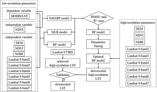
The thermal sharpen (TsHARP) model employs NDVI in a regression model to sharpen LST. It assumes that the relationship between LST and NDVI is the same at all scales [22]. Correlations between LST and NDVI are established [23], caused by shadows and evapotranspiration, which make vegetation surface cooler than bare soil [24]. The building process is shown in Figure 1.
The key to the TsHARP model is the determination of the most appropriate relationship between LST and NDVI through regression analysis. In this research, three regression models—linear regression, nonlinear binary curve regression and nonlinear ternary curve regression model—were used to fit the scatter distribution of LST and NDVI at a scale of 1 km. The fitting function is as shown in the following equation. From these three regression models, by comparing the R2 and RMSE, the best-fitting regression model can be used to predict the LST distribution at a scale of 100 m.
where , , and represent regression coefficients, and represents NDVI.
2.1.2. MLR Model
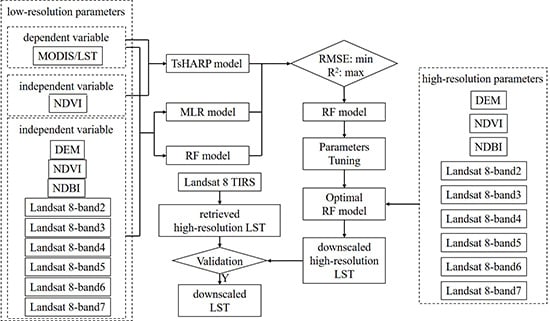
The multiple linear regression (MLR) model, shown in Figure 2, is based on multiple linear regression [25]. In downscaling low-resolution remote sensing products, additional high-resolution remote sensing information needs to be introduced to achieve downscaling conversion.
In the following building process, low-resolution parameters comprised two parts, namely, dependent and independent variables. LST was set as the dependent variable, and independent variables consisted of DEM, NDVI, NDBI, and band 2 to band 7 of Landsat 8. According to the low-resolution variables, we used the least squares method to build an MLR model, as shown in Equations (4) and (5) [26]. The LST at high resolution was estimated based on the p corresponding independent variable and multiple regression models.
where is the LST from low-resolution remote sensing products; (, , …, ) are several parameters, which are DEM, NDVI, NDBI and Landsat 8 OLI band 2 to band 7 at low-resolution; is the multiple linear regression model, and , , , …, are regression coefficients.
2.1.3. RF Model
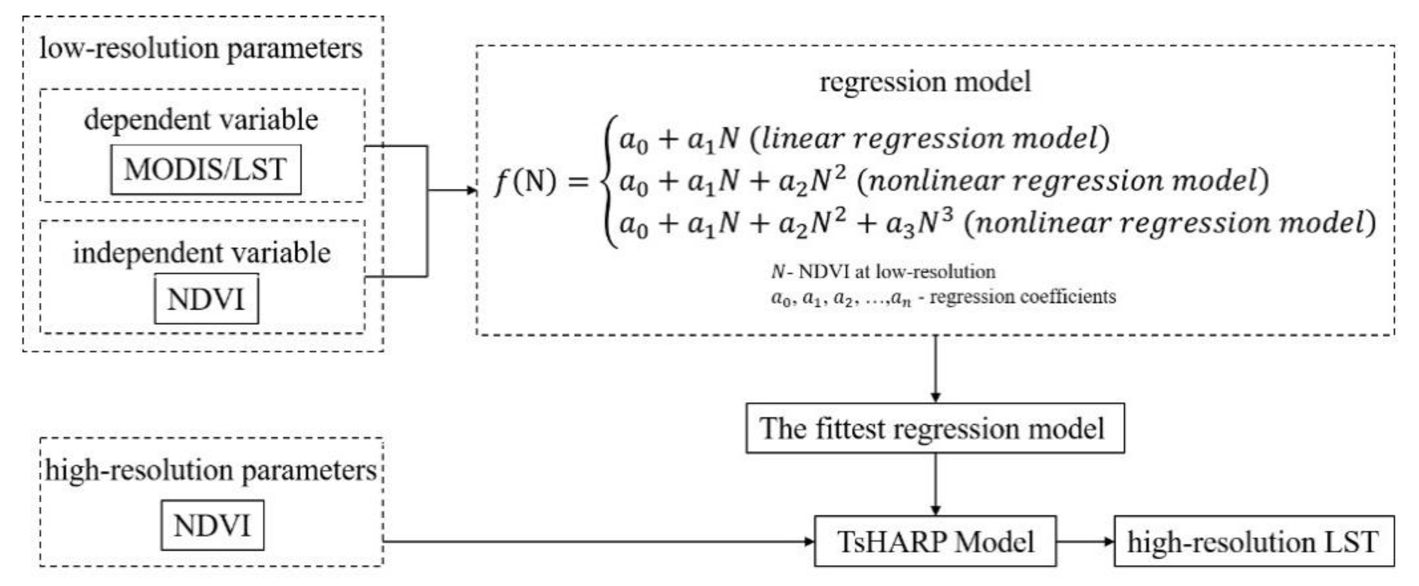
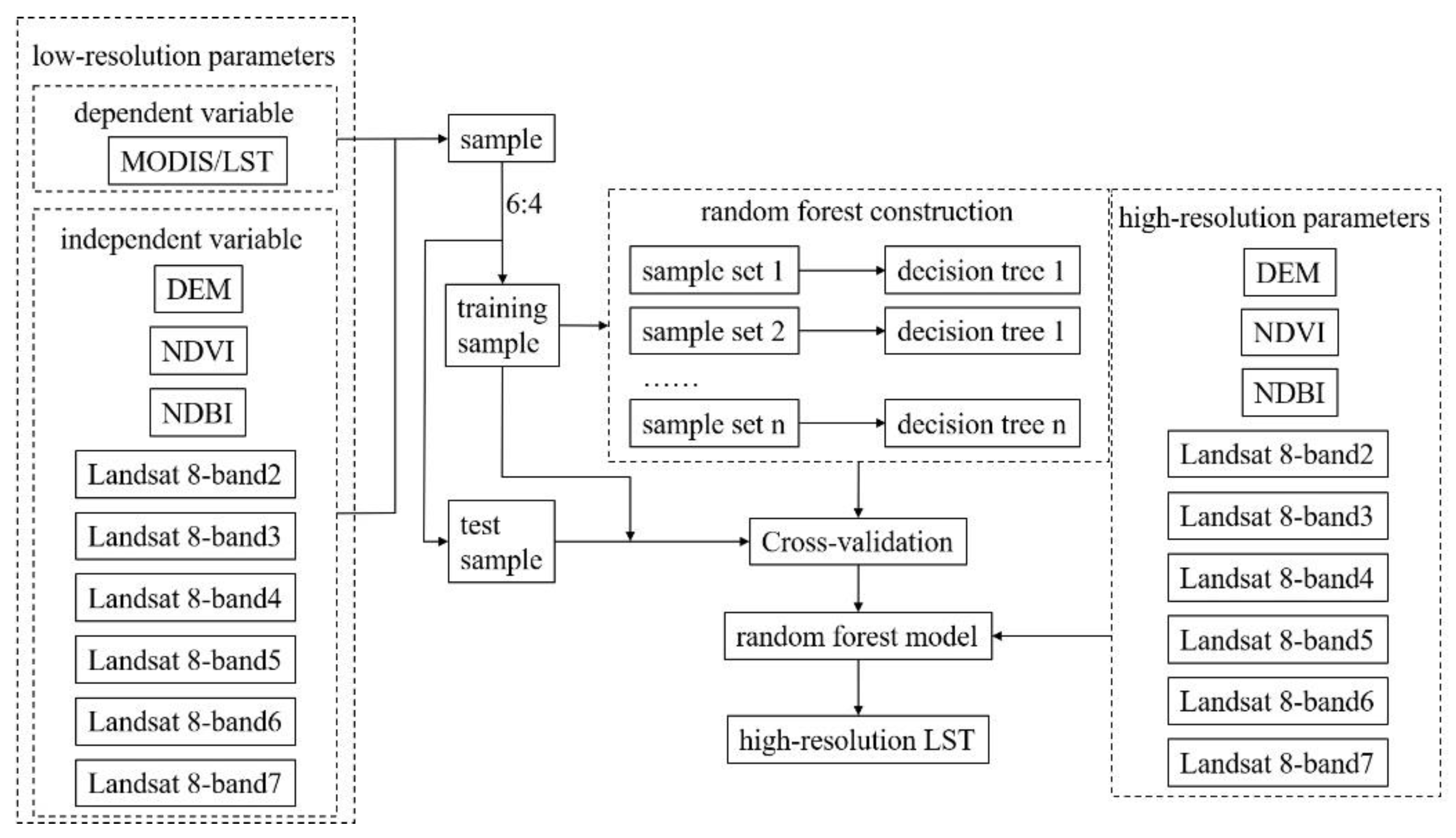
The random forest (RF) model is a machine learning model which prevents overfitting and was proposed by Breimans [27] in 2001. The term “random forest” was derived from the random decision forest proposed by Tin Kam Ho [28] in 1995. RF is a non-linear statistical ensemble method [29]. It uses bootstrap resampling technology to merge multiple samples extracted from the original training samples to generate a new series of training samples, then creates decision trees based on these training samples and establishes an RF model [15]. The RF model is not sensitive to multicollinearity, which can effectively prevent overfitting during the downscaling process [18]. The current research used Python 3.8 and the scikit-learn third-party open-source machine learning algorithm library, which is one of the most popular machine learning libraries [30].
Figure 3 shows the building process of the RF model. The training samples were remote sensing images with low resolution (1 km), and selection of dependent and independent variables was the same as that in the MLR model. In order to verify the accuracy of the models, we divided the sample into training samples and test samples according to a 6:4 ratio. The RF model was created by n decision trees generated by training samples. In the process of creating the model, several parameters needed to be adjusted, namely n_estimators, bootstrap, and oob_score of the RF framework parameters and max_features, max_depth, min_samples_leaf, min_samples_split, max_leaf_nodes, min_impurity_decrease, criterion and min_samples_leaf of the RF decision tree parameters [31]. Among these, n_estimators, max_depth and max_features were the three that most affect the downscaling result. In order to prevent the model from underfitting, we tuned these three parameters for fitting to achieve the optimal model. Then, we used the previously divided training samples for cross-validation based on the cross_val_score module in the scikit-learn libraries to determine the feasibility of the model.
2.2. Accuracy Evaluation and Fit Residual
Traditional quantitative evaluation usually uses one evaluation indicator. In order to compare the accuracy of the three downscaling models for each day and night during four seasons more objectively, this research used two evaluation indicators for comprehensive evaluation and analysis, R2 (coefficient of determination) and RMSE (root mean square error).
R2 (coefficient of determination) is an important statistic to reflect the model fit. In statistics, it is used to measure the proportion of dependent variables that can be explained by independent variables to determine the explanatory power of the regression model [32]. R2 takes values between 0 and 1 with no units. It is the most commonly used index to evaluate the pros or cons of regression models. The larger the value of R2 (closer to 1), the better the regression model is fitted.
RMSE (root mean square error) is a commonly used measure of the similarity between two vectors in n-dimensional space [33]. RMSE can test the consistency of real images and simulation images, and thus can be used to judge the effect of different downscaling models. The RMSE calculation is shown in Equation (6). Larger errors have a disproportionately greater effect on RMSE. Consequently, RMSE is sensitive to outliers [34]. RMSE is non-negative. A lower RMSE means higher consistency between simulation images and real images.
where the represents root mean square error, represents the low-resolution real images to reflect LST, represents the low-resolution simulation images to reflect LST, and is the total number of pixels in the low-resolution real images or simulation images.
In the process of establishing a correlation model at a low resolution, a residual exists between the real and simulation images. In order to improve the accuracy of the simulation of high-resolution LST images, this research fitted the residual to the simulation of high-resolution images. The flow chart is shown in Figure 4. A spline was used to interpolate adjacent cells to downscale the LST residual. The last step was to fit the high-resolution residual to the high-resolution simulation images, finally resulting in high-resolution land surface temperature images.
2.3. Downscaling Result Validation Based on Retrieved LST
To provide further confirmation of the approach, this research verified the downscaling accuracy using retrieved LST values from Landsat 8 TIRS with similar time and weather conditions as those of MODIS/LST. The single-channel algorithm proposed by Giannini et al. [35] and Dissanayake et al. [36] for LST retrieval of Landsat 8 TIRS has high accuracy and sensitivity.
Firstly, the proportion of vegetation was calculated using Equation (7) [37]:
where represents the proportion of vegetation; represents the normalized difference vegetation index (explained in Equation (9)); and represent the minimum and maximum value of NDVI, respectively.
Secondly, land surface emissivity was computed using Equation (8):
where represents land surface emissivity; represents the proportion of vegetation.
Finally, LST corrected for spectral emissivity was computed using Equation (9) [38]:
where represents land surface temperature; represents the at-satellite brightness temperature [39]; represents the band 10 wavelength in Landsat 8 TIRS (10.8 μm); is 1.438 × 10⁻² mK, and represents land surface emissivity.
Due to the difference between Terra satellite and Landsat 8 orbits, the revisit period of MOD11A2 is 8 days and that of Landsat 8 is 16 days, meaning that the images cannot be obtained in the same day. In addition, there is also an error of several minutes in the scanning time. In order to solve the contradiction in temporal resolution, we introduced meteorological conditions, including maximum and minimum air temperature, relative humidity, wind speed [40] and solar radiation [41] on the basis of selecting two adjacent dates as much as possible. Finally, we selected a set of downscaling LSTs and retrieved LSTs with the closest time and the most similar meteorological conditions to verify the downscaling method accuracy.
3. Case Study
3.1. Study Area
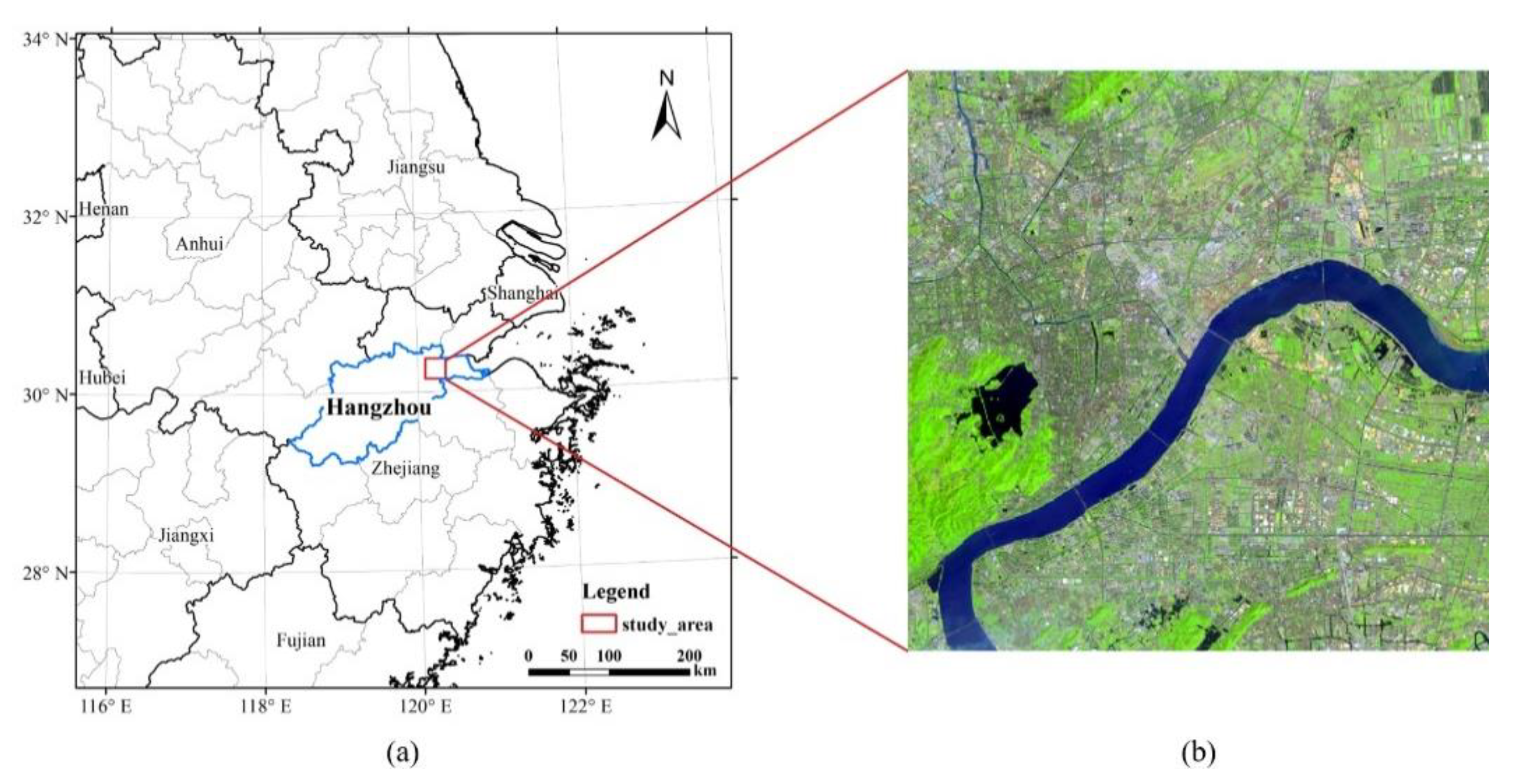
The study area is located in the center of Hangzhou, as shown in Figure 5. This research selected a square urban area with a side length of 25 km. Hangzhou is located in the central and southern areas of the Yangtze River Delta. Hangzhou’s climate is humid subtropical with four distinct seasons [42].
The study area includes various land use and land cover. Qiantang River runs through this area. West Lake is located on the west side. To the southwest of West Lake is a forest area. The urban area is mainly concentrated in areas to the north, east, and northeast of West Lake. As an important part of the urban agglomeration in the Yangtze River Delta, Hangzhou developed with rapid urbanization from the end of the previous century. Due to urban expansion and population growth, the urban structure has changed significantly. This has also led to climate change in this area, particularly in terms of SUHI. Previous research shows that SUHI is a significant contributor to regional warming in this area [43].
3.2. Data Source and Preprocessing
In this study, MODIS/LST products and Landsat 8 OLI were obtained from summer 2013 to spring 2014. Landsat 8 OLI provides seasonal coverage of global land images with nine bands. These remote sensing images use the World Reference System (WRS) to enable users to search for images from any part of the world using path and row numbers [44]. In Landsat 8 OLI, the coastal aerosol band (band 1) focuses on aerosols research in coastal areas; the panchromatic band (band 8) produces black and white images with a resolution of 15 m used to enhance and improve resolution; and the cirrus band (band 9) is designed for clouds, particularly for cirrus clouds [45]. These three bands were not useful for the downscaling of this study. In contrast to these bands, the visible blue band (band 2), green band (band 3) and red band (band 4) can help identify various land uses and land covers; the near-infrared band (band 5) provides vegetation indexes, such as NDVI, which allow measurement of plant health in combination with other bands; and the shortwave infrared bands (bands 6 and 7), which are particularly useful for distinguishing wet from dry earth, and for geology [45]. Thus, we only selected bands 2 to 7 from Landsat 8 OLI as the data source. Landsat 8 OLI is greatly influenced by clouds and weather. Accordingly, several sunny days without any clouds above the study area were chosen: April 14, July 19, November 8 in 2013 and January 27 in 2014. We selected Landsat 8 Level-1 Data Products after system radiation correction and geometric correction [39]. The WRS path and row were 119 and 039, respectively. The Landsat data we chose are shown in Table 1. The additional parameters at high-resolution extracted from Landsat 8 OLI were pre-processed according to Equations (10) and (11) [46,47]. Meanwhile, DEM data with a resolution of 30 m, which reflect the altitude situation, were also used in the RF model and the MLR model as independent variables. In order to downscale from 1 km to 100 m, this research resampled these parameters at a scale of 100 m and 1 km.
where RED, NIR and SWIR1 represent band 4, band 5 and band 6 in Landsat 8 OLI, respectively [39].
MOD11A2/LST products with a resolution of 1 km were selected as the low-resolution LST data with a temporal resolution of 8 days, including day data (10:30 a.m.) and night data (10:30 p.m.). MOD11A2 products were retrieved based on the split channel algorithm [48]. The path and row were 28/05 and 28/06, respectively. The imaging dates, shown in Table 1, were April 7, July 20, November 9 in 2013 and January 17 in 2014, similar to the Landsat 8 OLI dates. Then, the MODIS Tools called MRT were used for reprocessing tasks, such as creating a mosaic and resampling.
4. Results and Discussion
4.1. Model Selection and Precision Analysis
Based on SPSS and Python, we constructed correlation models for statistical low-resolution data. Downscaling based on the TsHARP and MLR models was run on SPSS, and the RF model was run using Python.
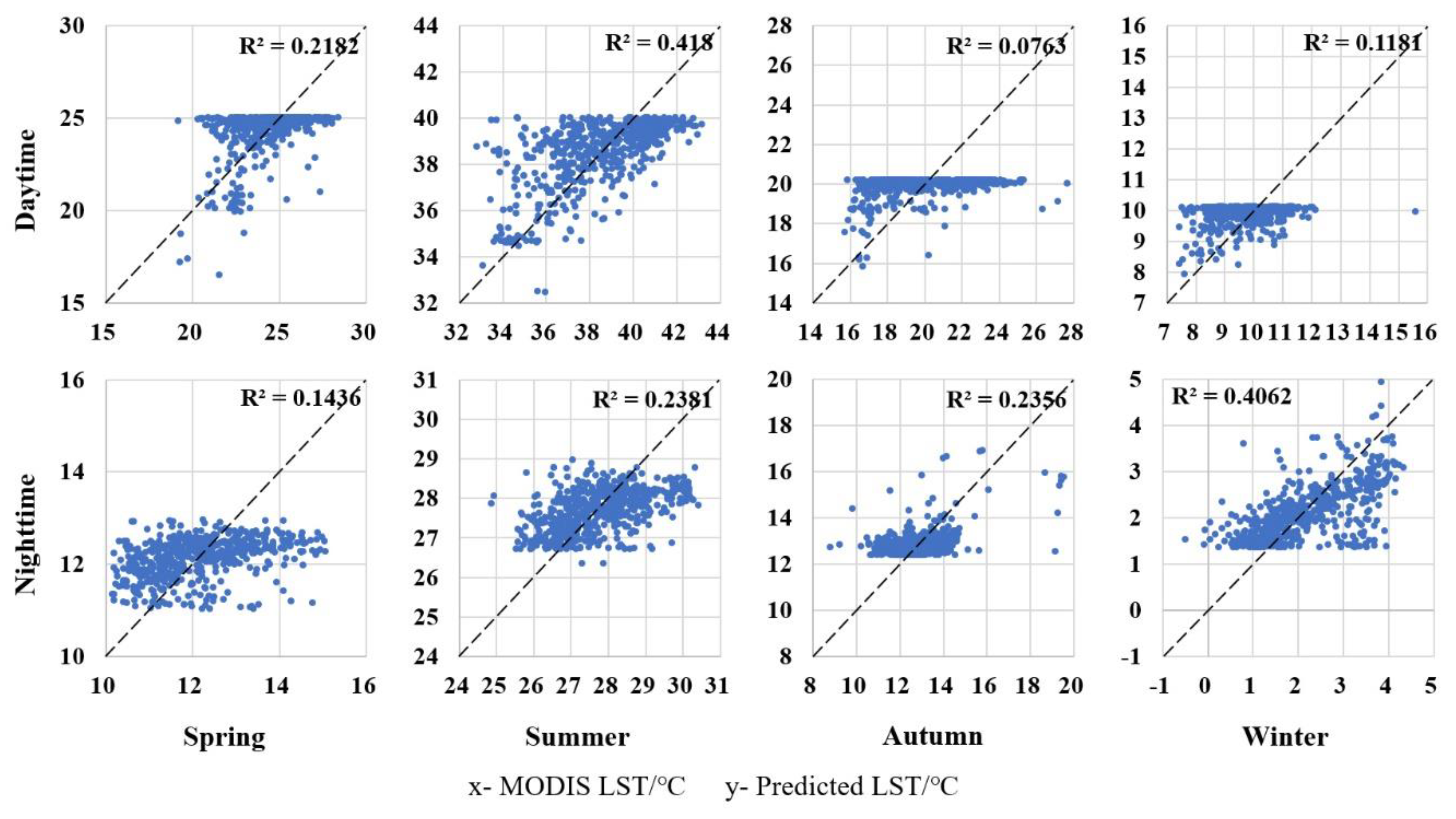
After statistical calculation, the TsHARP model with the best fitting was the third of three equations, the unary cubic model. Table 2 shows the regression coefficients of the TsHARP model during day and night in four seasons. According to these regression coefficients, we formed the corresponding downscaling models and thereby predicted low-resolution LST. Among the regression coefficients, a0 has high significance for the models regardless of the seasons or whether day or night; a2 and a3 have low significance, especially in autumn and winter daytime. Figure 6 shows the scatter plot of predicted LST data based on the TsHARP models versus MODIS LST data. The x-axis represents the MODIS/LST product values, which are the true LST (1 km level); the y-axis represents the predicted LST from the TsHARP model (1 km level).
Scatter points were not distributed near the 1:1 line, which meant that this model was poor and could not be used in downscaling research in this study area. The TsHARP model is based on the correlation between LST and NDVI. Due to shadows and transpiration, the vegetation surface is usually cooler than that of other landscapes [24]. This theoretical basis had considerable errors because of the strong spatial heterogeneity of the study area [49,50,51], and the predicted LST had an obvious boundary value. Therefore, the TsHARP model was not suitable for this study.
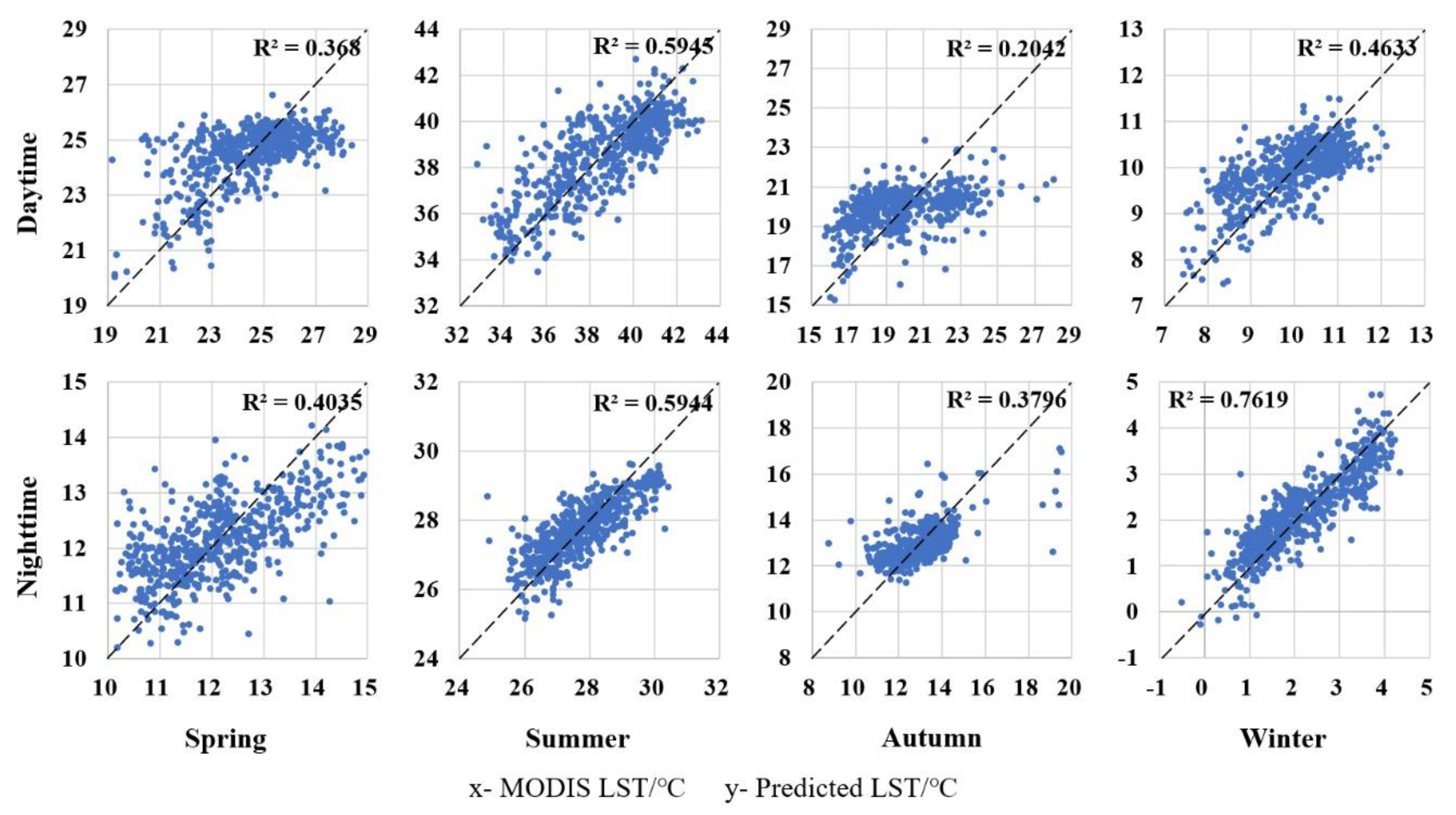
In order to solve the problem of the sharp drop in the correlation between LST and NDVI due to spatial heterogeneity, we introduced more independent variables to build the MLR model based on NDVI, including DEM, NDBI, and Landsat B2 to B7. According to the independent and dependent variables, we calculated the regression coefficients (a0, a1, a2 … an) using the least-squares method. Table 3 shows the regression coefficients of the MLR models. Overall, CT, DEM, NDVI, B2, B3, B4, and B7 have high significance, compared with other variables. The significance of NDBI during the day is generally higher than that at night. Scatter diagrams comparisons of MODIS LST and predicted LST (Figure 7) show that the predictive capabilities of the MLR model are improved compared with the TsHARP model. However, since the MLR model is a linear model, which cannot easily characterize the complex nonlinear regression between LST and independent variables, there are a large number of outliers. Thus, the MLR model is not a perfect downscaling model in this research.
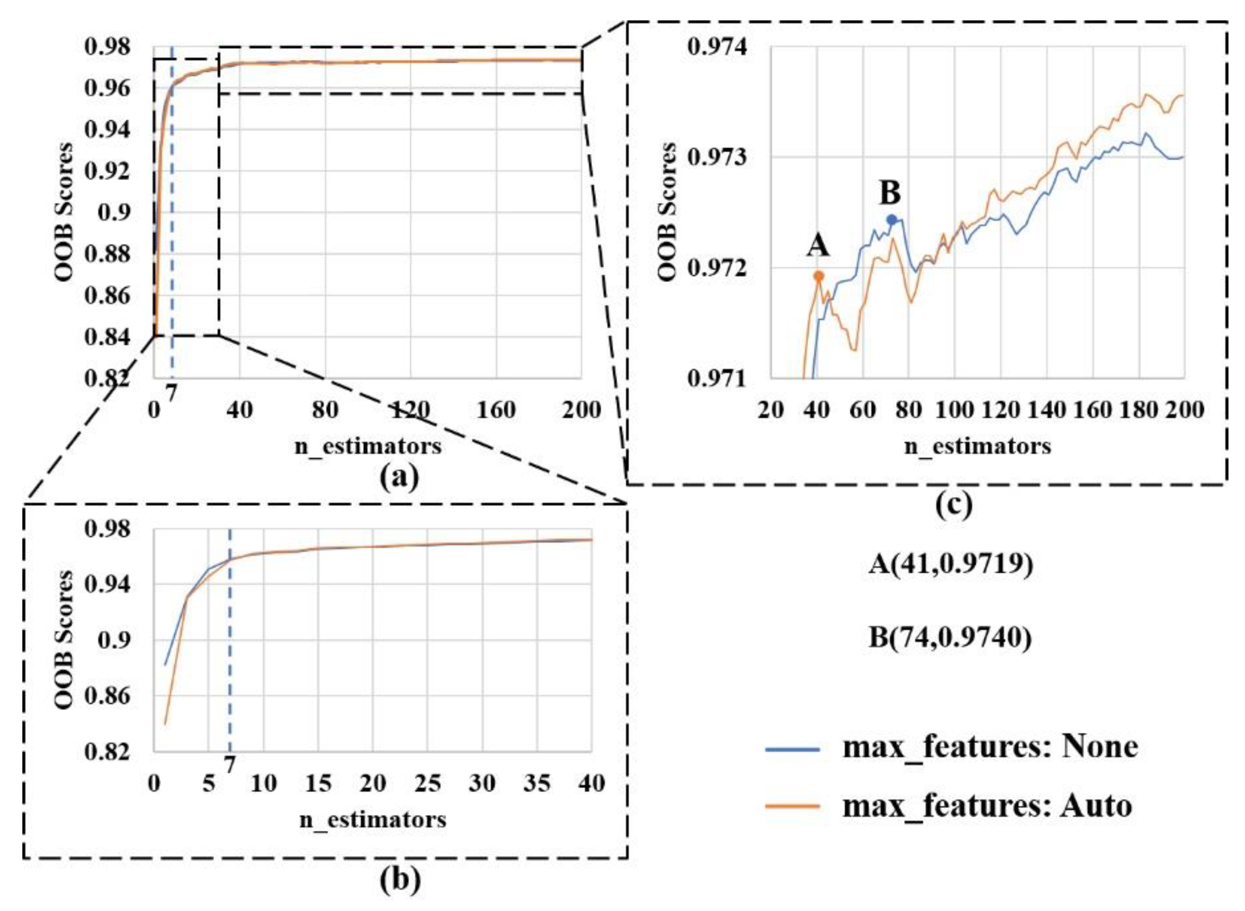
The simple single-factor and multi-factor regression models cannot completely summarize the complex relationship between different factors and LST. Under the premise that the physical mechanism is still unclear, a better choice is to build a downscaling model with the help of machine learning methods. Compared with some other machine learning methods, such as artificial neural networks and support vector machines, the RF model has the advantages of low computation needs and a large number of samples, which are appropriate for downscaling research. The training process of the RF model mainly comprises the process of adjusting hyperparameters, which is generally called parameter tuning. Various parameters combinations will have different predicted results. Therefore, there is no single set of parameters that can optimize the various models. Optimization requires continuous training and adjustment to achieve the optimal combination for a certain type of problem [52]. We tuned parameters according to the importance of the three most significant parameters, which are n_estimators, max_depth and max_features. Due to the small number of samples in this research, the division depth was not constrained; that is, max_depth was set to “None”. Thus, this study only tuned n_estimators and max_features. Other parameters were set to default values. Figure 8 shows the changes of the model’s obb score, that is R2, when tuning n_estimators and max_features in three parts: Figure 8a represents the changes with n_estimators ranging from 1 to 200; Figure 8b represents the partial enlarged detail with n_estimators ranging from 1 to 40, and Figure 8c represents the range from 30 to 200.
In order to prevent underfitting of the RF model, in the tuning process, we increased n_estimators to improve the model’s fitting ability; when the Out Of Bag (OOB) scores did not significantly improve for the first time, the value of n_estimators was optimal (Point A and B in Figure 8). Meanwhile, we adjusted max_features and set it to None (blue line in Figure 8; max_features are the square root of the sample features) and Auto (orange line in Figure 8; max_features are the sample features).
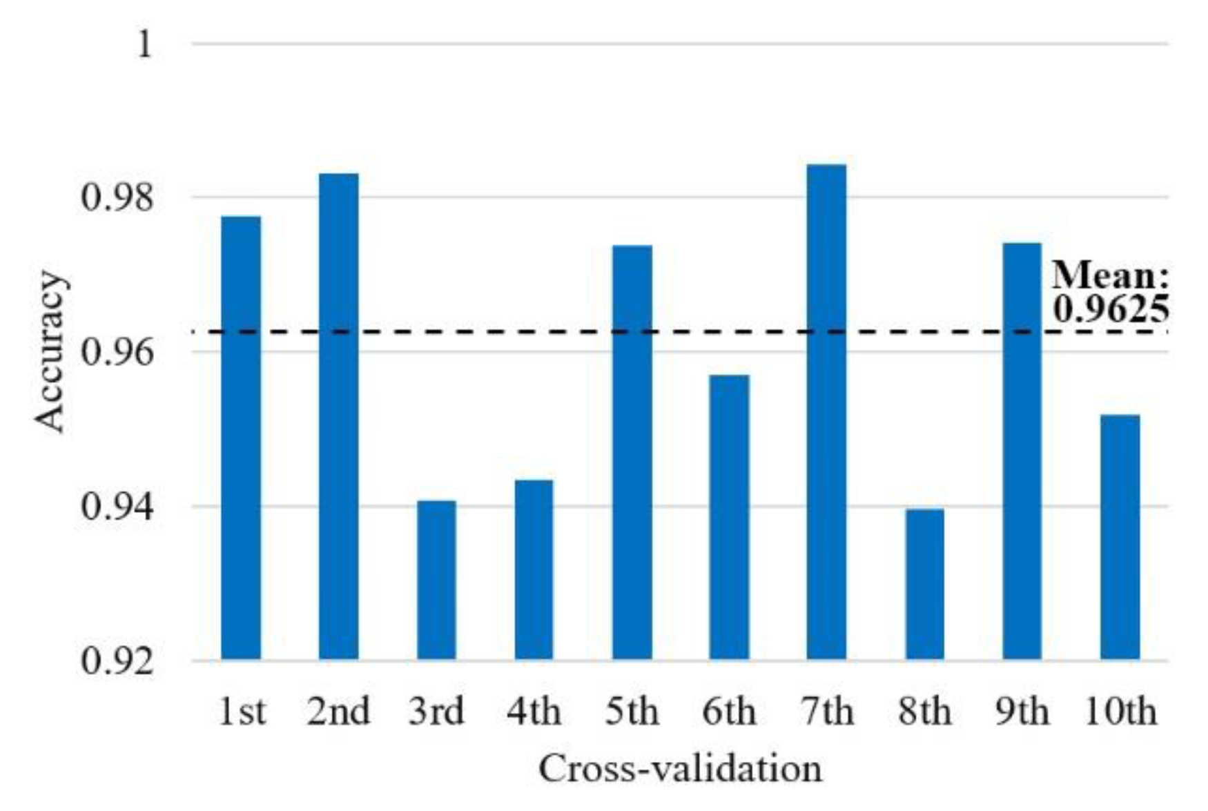
Combining the predicted results of the above two models, the fitting degree of winter night was the highest. Thus, we took winter night as an example of parameter tuning. When all parameters were set to default values, the OOB score was 0.9621. When n_estimators increased from 1 to 7, OOB scores rose rapidly, then tended to be flat. According to Figure 8c, the orange line reached the first maximum OOB scores (OOB score = 0.9719), Point A, when n_estimators was 41. When n_estimators was 71, the first maximum OOB score of the blue line was 0.9740, Point B. Consequently, Point B was the best parameter combination as shown in Table 4. After parameter tuning, we obtained the optimal combination corresponding to an OOB score of 0.9740, which was 0.0119 higher than the original OOB score. Then, we combined the training samples and test samples to perform a total of 10 cross-validation on the optimal model based on the cross_val_score module to verify whether the model was good fitting. The 10-fold cross-validation results are shown in Figure 9. The mean of accuracy was about 0.9625. The fourth cross-validation had the highest accuracy, of about 0.9834, and the lowest was the ninth, of about 0.9396. The mean squared error (MSE) of the training sample was about 0.025 °C and that of the test sample was about 0.053 °C. The MSE of test samples was slightly higher than that of training samples, indicating that the model was not overfitting. Overall, the cross-validation results meet the requirements; that is, the optimal RF model could be used in the subsequent downscaling research.
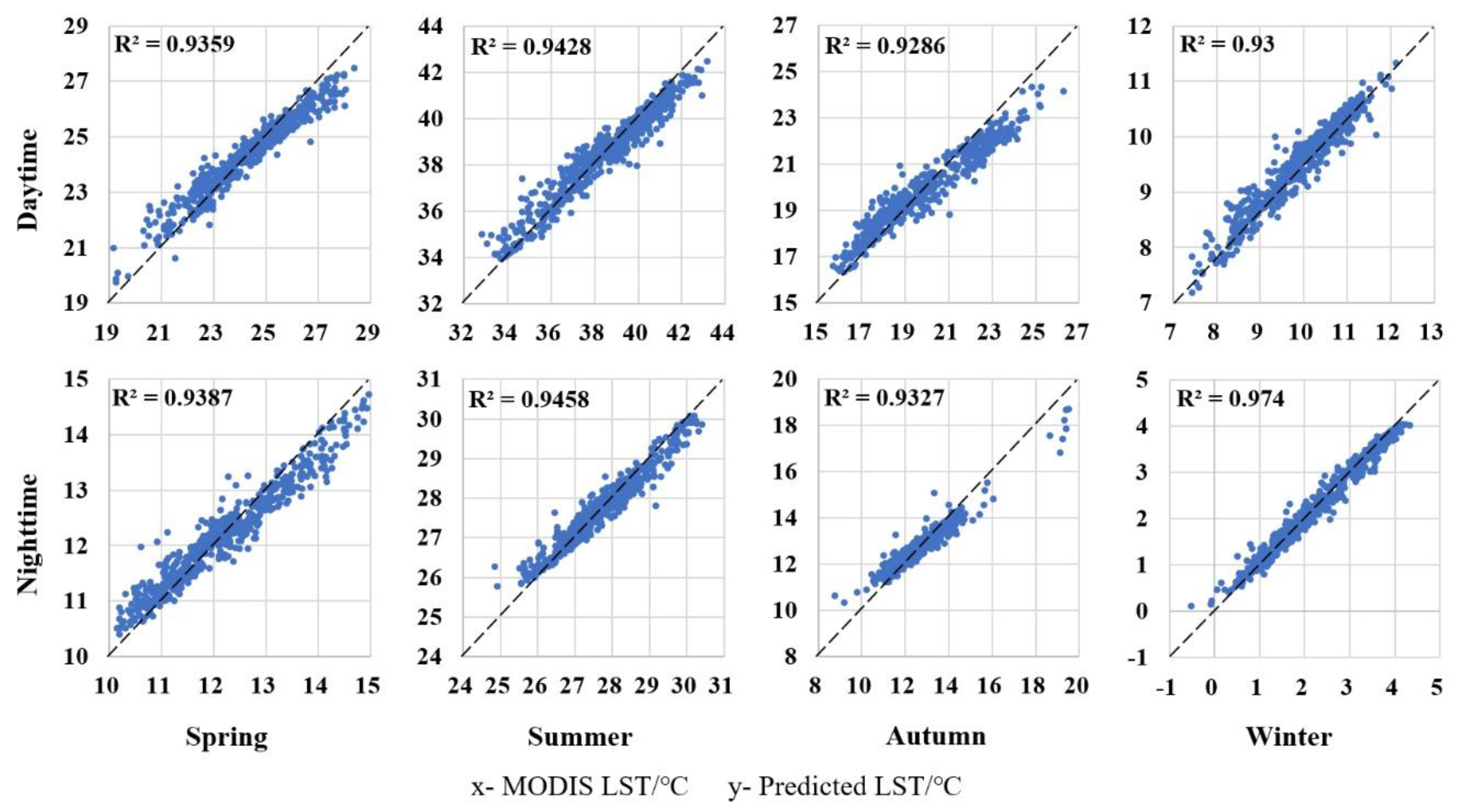
Through the above method, we tuned the parameters of the RF models for different dates so that their accuracy complied with the requirement based on cross-validation; we then predicted low-resolution LST based on these RF models and compared results with MODIS/LST products to verify model accuracy. The scatter diagrams are shown in Figure 10. The scatterplot comparisons of MODIS LST and predicted LST show the improved predictive capabilities of the RF model in comparison to the TsHARP and MLR models, with almost all scatter points clustered around the 1:1 line and fewer outliers. Compared with the earlier two models, the RF model is more suitable for downscaling in this highly heterogeneous research region. Furthermore, the error histograms (Figure 11) show that the prediction errors of the RF model approximately obeyed the normal distribution; the peak value appeared around 0 °C, and values gradually decreased on both sides. Peaks at night were generally higher than those during the daytime. The prediction errors in summer and winter were significantly less than those in spring and autumn, especially during daytime. The daytime errors in autumn were more discrete than those during other seasons. Compared to the minimum value, the value of winter night was closest to 0 °C, respectively, −0.7 °C and 0.5 °C. However, 1% of values were less than −2 °C, and 0.2% of values were more than 2 °C.
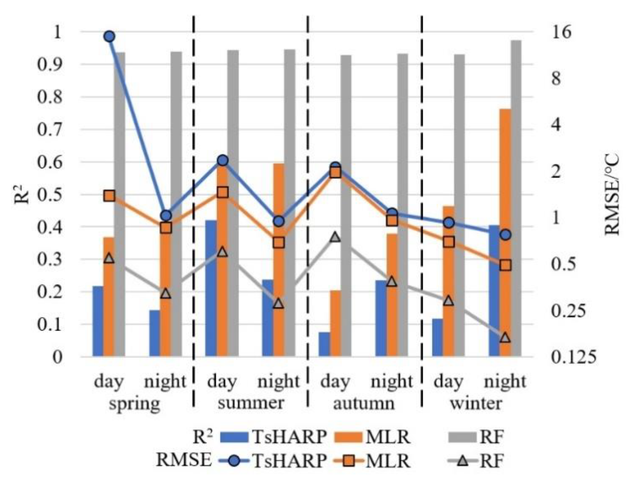
To summarize, R2 and RMSE were calculated for MODIS/LST products and predicted LST, as shown in Figure 12. The histogram shows R2, and the line chart shows RMSE, of various models. Blue, orange, and gray represent the TsHARP, MLR, and RF models, respectively. The results clearly show that the RF model was more suitable for this research than the TsHARP and MLR models. This is evident in the significantly higher R2 and lower RMSE of the RF model compared to the other two models. For the RF model, the prediction effect at night was better than that during the daytime, and that at winter night was the best, with R2 of 0.9740 and RMSE of 0.1678. The worst effect was for autumn daytime: R2 was 0.9286 and RMSE was 0.7556. However, even the worst RF model performed better than the other two models. From a seasonal perspective, R2 values in summer and winter were higher than those in spring and autumn. From low to high, RMSE values were winter, spring, summer, and autumn. By comparison with the single-factor TsHARP model, the prediction improvement of the MLR model with more independent variables was limited due to the simple linear regression. The application of the RF model greatly enhanced the model’s predictive capabilities, because, under the premise of multiple factors, machine learning could perform complex nonlinear regression. According to the above model selection and precision analysis, we only selected the RF model to undertaken downscaling of MODIS/LST products from 1 km to 100 m.
4.2. Downscaling Results and Surface Urban Heat Island
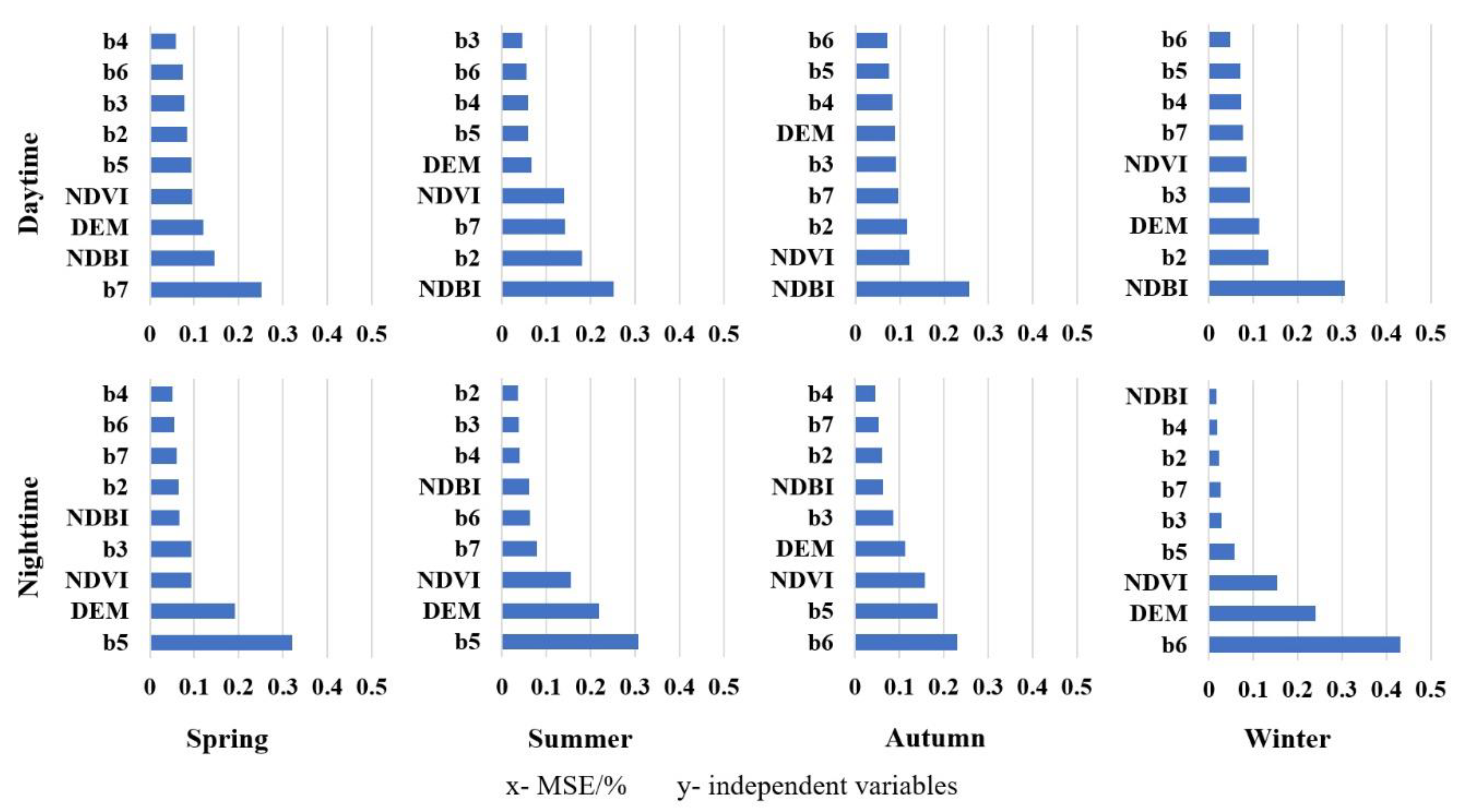
During the construction of nonlinear regression models, the RF model was able to provide feature importance based on randomized variable selection. The importance scores were presented in mean squared error (MSE). The larger the MSE of an independent variable, the more important that variable is to a model [54]. Figure 13 shows the independent variable importance scores from all research data; the x-axis represents MSE, and the y-axis represents the independent variables. Among the independent variables, b2 to b7 represent Band 2 to Band 7 from Landsat 8 OLI. During daytime, the importance scores of various factors were relatively balanced, and the difference between high and low score factors was large at night, especially at winter night. The b6 score reached 43.2%; in comparison, the highest score in daytime was 30%, for NDBI in winter. At night, b5 and b6 were the most important, with high scores. Meanwhile, DEM played a major role in the RF models at night. Contrary to nighttime, DEM scores in daytime were not large. According to the Environmental Lapse Rate [55], high-altitude areas usually received more solar radiation with more xeric and warmer conditions, particularly north-facing slopes. In the current research, different orientations resulted in a significant difference of LST. Therefore, the effect of DEM is weak when receiving solar radiation [56]. NDBI during daytime played a key role in the RF models, with the highest scores in summer, autumn and winter and the second highest in spring. This meant that buildings heated by solar radiation had a significant influence on LST. By contrast, at night without solar radiation, NDBI had lower importance scores than DEM.
The intention of an LST downscaling model is to overcome the contradiction between the spatial–temporal resolutions of various remote sensing images to obtain LST products with high spatial–temporal resolution. According to the RF models constructed in Section 4.1, we downscaled MODIS/LST from 1 km to 100 m; that is, independent variables with a scale of 100 m were used to predict the corresponding LST. In order to improve prediction accuracy and reduce errors, we used a spline method to fit residuals, as introduced in Section 2.2. Due to some restrictions of the study area, MODIS/LST products could not provide high-resolution LST of Qiantang River, which crosses the urban area, mostly resulting in a lack of water surface temperature data. The data were unable to provide enough training samples for the RF model. Therefore, the downscaling accuracy based on the RF model of water surfaces will be greatly reduced. The average annual sediment discharge was 6.68 million tons [57]. The tidal bore is one of the symbolic features of the Qiantang River. The effect of tidal bores causes abrupt changes of the river bed, thus changing the land cover, which in turn influences LST [58]. Hence, we eliminated the LST downscaling of large areas of water, such as Qiantang River and West Lake.
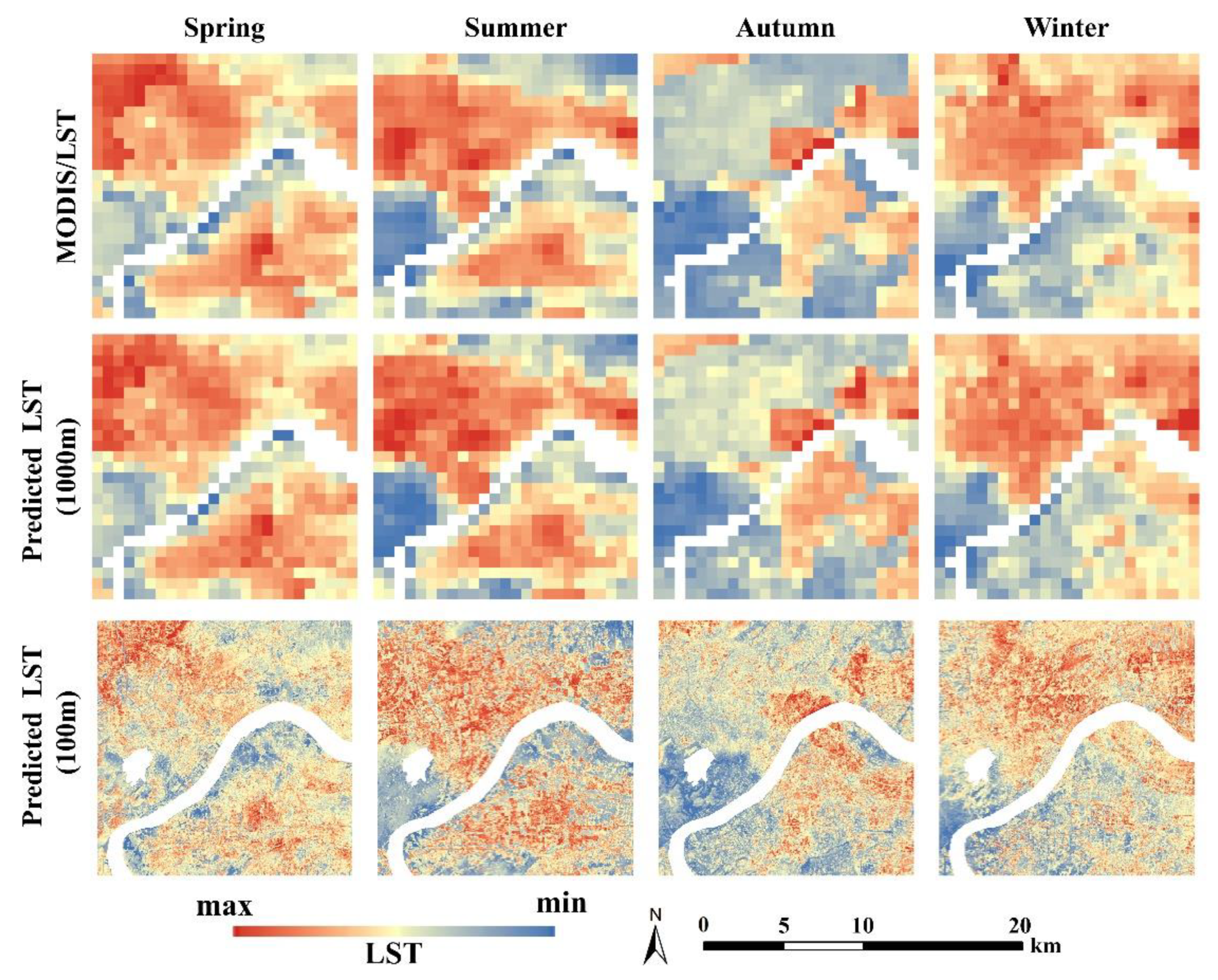
Figure 14 and Figure 15 show LST distribution during day and night, respectively, including the MODIS/LST products, predicted LST with a scale of 1 km, and predicted LST with a resolution of 100 m; the latter two represent the downscaling results. LST changes from blue to red. Blue regions represent low-temperature areas, and red regions represent high-temperature areas. Comparing MODIS/LST products and predicted LST with a scale of 1 km, the similarity of each pair of images is extremely high, whether during the day or at night, which also shows that the RF model is suitable for future downscaling research in this study area. The following prediction results, with a scale of 100 m, are the downscaling results after the fitting of residuals. The distribution of downscaled LST is basically consistent with the distribution of MODIS/LST products.
With the exception of autumn, the SUHI distribution during the day is similar across the seasons. On the north bank of the river and the northeast side of the lake, a large number of high-temperature areas are generally distributed. The LST of the southwest area of the lake is lower than that of the other areas. Compared with spring and summer, there are more high-temperature areas in the northeast corner of the region and the north bank of the river. However, the low-temperature areas in the southern part of the river are more than those in spring and summer. In contrast to spring, summer and winter, the high-temperature areas in autumn are obviously fewer. Red areas mainly appear on the north bank of the river and near the east side of the research region. Similar to the other three seasons, the low-temperature areas are also located at the southwest of the lake.
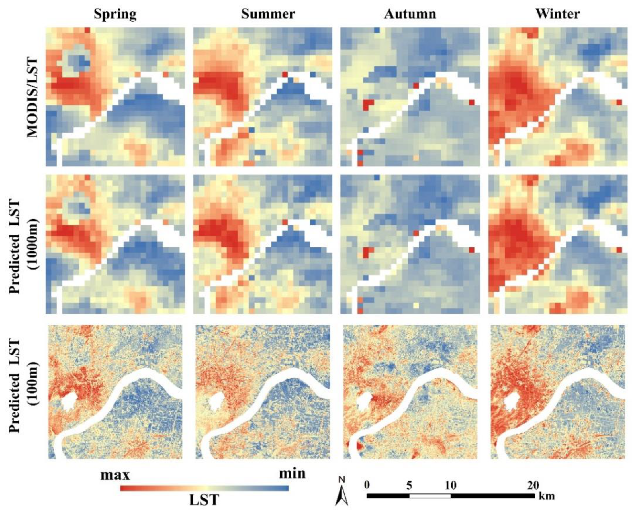
At night, high-temperature areas are mainly concentrated around the lake in low-resolution MODIS/LST products. However, SUHI in autumn is obviously different from other seasons. Several small areas with extremely high temperatures can be found in MODIS/LST products. Through downscaling and excluding large water areas including West Lake and Qiantang River, the corresponding high-resolution LST shows that the SUHI distributions at night are similar in all seasons. The blue areas are located in the northeast of the study area and the south bank of the river. The dissimilarity in the four seasons lies in the relative differences of LST in high-temperature areas. The red area is larger in winter than in other seasons.
From the downscaling results, we found that there are significantly more high-temperature areas during the day than at night. This means that the distribution range of SUHI is wider during the day than at night. During the daytime, SUHI spreads throughout the research region, but at night, SUHI shrinks towards the West Lake and the south of the study area. Two obvious SUHI areas are distributed on both sides of Qiantang River. The LST of SUHI on the north bank is higher than that on the south bank. In daytime, the urban center, which is to the northeast of West Lake, is not clearly the warmest area; however, at night, the urban center became the core zone of SUHI irrespective of the season.
Ranges of LST during daytime (Figure 14) and at night (Figure 15) are shown in Table 5. Comparing MODIS/LST and predicted LST with a scale of 1 km, we found that the average LSTs were almost equal, with differences less than 0.02 °C. However, the ranges were smaller. Comparing MODIS/LST and predicted LST with a scale of 100 m, the mean LST difference showed improvement compared with the former, but within the allowable range. Furthermore, the LST ranges were close to those of MODIS/LST. The predicted LST (100 m) difference was largest in autumn during both day and night; that is, SUHI in autumn is the most serious. The difference in winter was the smallest. Generally speaking, differences during the day were always greater than those at night, and differences ranged from 2 °C to 5 °C, except in winter. In winter, the difference at night was 0.39 °C higher than that during the day. From the mean LST throughout the year, LST rose sharply to reach 38.42 °C in the daytime and 27.56 °C at night from spring to summer, then gradually decreased to 9.91 °C during the day and 1.98 °C at night in winter.
4.3. Validation Results Comparing Downscaling LST and Retrieved LST
Due to satellite orbit restrictions, we could not obtain MODIS/LST products and Landsat 8 OLI/TIRS to retrieve LST with high resolution with the same scan time. We referred to historical meteorological dates from Greenhouse Data [59] as shown in Table 6. According to the date, we preliminarily excluded spring and winter, because the acquisition dates of Landsat 8 OLI/TIRS and MOD11A2 were too far apart. Compared with spring and winter, the dates in summer and autumn were adjacent. The scan times [8,60] of the two remote sensing types was similar, concentrated around 10:30 a.m., and only 2 or 3 min apart. Then, we organized and analyzed the obtained meteorological data. The smallest difference was in summer (with an asterisk in Table 6). The maximum and minimum air temperatures differed by only 1 °C; the difference in relative humidity was 1%; the wind speed difference was 0.1 m/s; and the solar radiation difference was about 0.4 MJ/m2. Compared with other sets of data, we selected the Landsat 8 TIRS on July 19 2013 to retrieve LST and combined with MOD11A2 on July 20 to verify downscaling accuracy.
Using the single-channel algorithm in Section 2.3, the retrieved LST (that is, the real LST) with a resolution of 30 m is shown in Figure 16b. Figure 16a shows the downscaled LST with a resolution of 100 m. The differences in the LST ranges of the two figures is small; the real LST ranges from 34.89 °C to 41.62 °C, while the other ranges from 33.18 °C to 42.82 °C. According to the LST distribution, the high-temperature areas (red areas) and low-temperature areas (blue areas) are basically similar. From the comparison of the downscaled and real LST, we present the error distribution histogram as shown in Figure 16c. The x-axis represents the error between the two types of LST, and the y-axis represents the number of pixels. The error is approximately normally distributed. The peak value of the error is around 0.3 °C, the mean of errors is about 0.2617 °C, the median is about 0.3 °C, and the standard deviation is about 1.56 °C. Since the scan times and scan methods of Landsat 8 TIRS and MODIS/LST are different, as mentioned above, and the meteorological conditions at the two times were not exactly the same, a few errors between the downscaled and real LST. This small number of errors meets the research requirement; that is, the downscaled LST based on the RF model meets the accuracy requirement, and the RF model can be used in downscaling research.
5. Conclusions
This research used three different models (TsHARP, MLR and RF models) to downscale MODIS/LST products from 1 km to 100 m based on Landsat 8 OLI and a DEM with high-resolution data and selected the highly heterogeneous Hangzhou urban area as the research region. Of the three model types examined, the TsHARP model was a single-factor regression model that favors nonlinearity based on the correlation between LST and NDVI. The MLR model was a multi-factor linear regression model, which introduced more independent variables compared to the TsHARP model, including DEM, NDBI and Landsat 8 OLI Band 2 to Band 7. The RF model was used as a multi-factor nonlinear regression model based on machine learning to predict LST. Then, we used R2 and RMSE to evaluate the prediction effect of these three models. According to the evaluation comparison, the suitable model—that is, the RF model—was selected for the subsequent downscaling study. After parameter tuning, we built the optimal RF model to downscale the MODIS/LST products for four seasons during day and night and analyzed SUHI based on the high-resolution LST. Finally, we selected similar retrieved LST based on Landsat 8 TIRS to verify the feasibility of the RF model.
However, the choice of independent variables in this research was flawed. This article selected DEM, NDVI, NDBI and Landsat 8 OLI Band 2 to Band 7, thus including only two topography-derived variables, NDVI and NDBI. In other studies, Hamid and Mohsen [61] selected RVI, DVI, RDVI, NDVI, SAVI and MSAVI, while Wei Z. et al. [62] chose NDVI, EVI, NDWI, LAI, ALB, ELV and SLP. In precision evaluation, we were unable to retrieve high-resolution LST based on Landsat 8 TIRS for the same periods to verify downscaling accuracy because the Terra Satellite, which provides MODIS/LST products, and Landsat 8 OLI/TIRS are not synchronized. We were only able to select a few high-resolution LST data at particular times to verify the downscaling accuracy.
We concluded that the proposed RF model downscaling method, based on the multi-factor nonlinear regression of LST and DEM, NDVI, NDBI and Landsat 8 OLI Band 2 to Band 7, was proven to be effective and flexible in downscaling the LST spatial resolution from 1 km to 100 m for various seasons in the research region. Compared to the downscaling methods based on the TsHARP model with single-factor nonlinear regression and the MLR model with multi-factor linear regression, both statistics and visual analysis supported this conclusion. According to the prediction precision, the RF model effects in winter and summer were slightly better than those in spring and autumn, and those at night were better than those during the day. Combined with high-resolution LST, we concluded that SUHI was spread throughout the city across a large area, with the exception of the hills to the southwest of West Lake. At night, SUHI shrank sharply in the urban center around West Lake and the low-temperature area increased. According to the LST difference across the four seasons, we found that SUHI was the most obvious in autumn and the weakest in winter. Finally, the error distribution histogram between the downscaled and real LST supported the conclusion that the RF model can be applied to downscaling research in highly heterogeneous regions.
Author Contributions
Onceptualization, R.W. and W.G.; formal analysis, R.W. and W.P.; methodology, R.W.; writing—original draft, R.W.; writing—review and editing, W.G. and W.P. All authors have read and agreed to the published version of the manuscript.
Funding
This research was funded and supported by the Key Technologies Research and Development Program, grant number 2018YFE0106100.
Conflicts of Interest
The authors declare no conflict of interest.
References
- Weng, Q.; Lu, D. A sub-pixel analysis of urbanization effect on land surface temperature and its interplay with impervious surface and vegetation coverage in Indianapolis, United States. Int. J. Appl. Earth Obs. Geoinf. 2008, 10, 68–83. [Google Scholar] [CrossRef]
- Stathopoulou, M.; Cartalis, C. Downscaling AVHRR land surface temperatures for improved surface urban heat island intensity estimation. Remote Sens. Environ. 2009, 113, 2592–2605. [Google Scholar] [CrossRef]
- Zakšek, K.; Oštir, K. Downscaling land surface temperature for urban heat island diurnal cycle analysis. Remote Sens. Environ. 2012, 117, 114–124. [Google Scholar] [CrossRef]
- Kustas, W.; Anderson, M. Advances in thermal infrared remote sensing for land surface modeling. Agric. For. Meteorol. 2009, 149, 2071–2081. [Google Scholar] [CrossRef]
- Chunqiao, S.; Songcai, Y.; Gaohuan, L.; Linghong, K.; Xinke, Z. The spatial pattern of soil moisture in Northern Tibet based on TVDI method. Prog. Geogr. 2011, 30, 569–576. [Google Scholar]
- Anderson, M.C.; Allen, R.G.; Morse, A.; Kustas, W.P. Use of Landsat thermal imagery in monitoring evapotranspiration and managing water resources. Remote Sens. Environ. 2012, 122, 50–65. [Google Scholar] [CrossRef]
- Ha, W.; Gowda, P.H.; Howell, T.A. A review of downscaling methods for remote sensing-based irrigation management: Part I. Irrig. Sci. 2013, 31, 831–850. [Google Scholar] [CrossRef]
- EarthExplorer. Available online: https://earthexplorer.usgs.gov/ (accessed on 17 April 2020).
- Quan, J.; Zhan, W.; Chen, Y.; Liu, W. Downscaling remotely sensed land surface temperatures: A comparison of typical methods. Yaogan Xuebao J. Remote Sens. 2013, 17, 361–387. [Google Scholar]
- Zhan, W.; Chen, Y.; Zhou, J.; Wang, J.; Liu, W.; Voogt, J.; Zhu, X.; Quan, J.; Li, J. Disaggregation of remotely sensed land surface temperature: Literature survey, taxonomy, issues, and caveats. Remote Sens. Environ. 2013, 131, 119–139. [Google Scholar] [CrossRef]
- Kustas, W.P.; Norman, J.M.; Anderson, M.C.; French, A.N. Estimating subpixel surface temperatures and energy fluxes from the vegetation index–radiometric temperature relationship. Remote Sens. Environ. 2003, 85, 429–440. [Google Scholar] [CrossRef]
- Agam, N.; Kustas, W.P.; Anderson, M.C.; Li, F.; Neale, C.M. A vegetation index based technique for spatial sharpening of thermal imagery. Remote Sens. Environ. 2007, 107, 545–558. [Google Scholar] [CrossRef]
- Essa, W.; Verbeiren, B.; van der Kwast, J.; Van de Voorde, T.; Batelaan, O. Evaluation of the DisTrad thermal sharpening methodology for urban areas. Int. J. Appl. Earth Obs. Geoinf. 2012, 19, 163–172. [Google Scholar] [CrossRef]
- Weng, Q.; Fu, P.; Gao, F. Generating daily land surface temperature at Landsat resolution by fusing Landsat and MODIS data. Remote Sens. Environ. 2014, 145, 55–67. [Google Scholar] [CrossRef]
- Hutengs, C.; Vohland, M. Downscaling land surface temperatures at regional scales with random forest regression. Remote Sens. Environ. 2016, 178, 127–141. [Google Scholar] [CrossRef]
- Bonafoni, S. Downscaling of Landsat and MODIS land surface temperature over the heterogeneous urban area of Milan. IEEE J. Sel. Top. Appl. Earth Obs. Remote Sens. 2016, 9, 2019–2027. [Google Scholar] [CrossRef]
- Govil, H.; Guha, S.; Dey, A.; Gill, N. Seasonal evaluation of downscaled land surface temperature: A case study in a humid tropical city. Heliyon 2019, 5, e01923. [Google Scholar] [CrossRef] [Green Version]
- Junwei, H.; Shanyou, Z.; Guixin, Z. Downscaling land surface temperature based on random forest algorithm. Remote Sens. Land Resour. 2018, 30, 78–86. [Google Scholar]
- Zhan, W.; Chen, Y.; Wang, J.; Zhou, J.; Quan, J.; Liu, W.; Li, J. Downscaling land surface temperatures with multi-spectral and multi-resolution images. Int. J. Appl. Earth Obs. Geoinf. 2012, 18, 23–36. [Google Scholar] [CrossRef]
- Peckham, R.; Gyozo, J. Development and Applications in a Policy Support Environment Series: Lecture Notes in Geoinformation and Cartography; Springer: Berlin/Heidelberg, Germany, 2007. [Google Scholar]
- Macarof, P.; Statescu, F. Comparasion of ndbi and ndvi as indicators of surface urban heat island effect in landsat 8 imagery: A case study of iasi. Present Environ. Sustain. Dev. 2017, 11, 141–150. [Google Scholar] [CrossRef] [Green Version]
- Sattari, F.; Hashim, M.; Pour, A.B. Thermal sharpening of land surface temperature maps based on the impervious surface index with the TsHARP method to ASTER satellite data: A case study from the metropolitan Kuala Lumpur, Malaysia. Measurement 2018, 125, 262–278. [Google Scholar] [CrossRef]
- Petropoulos, G.; Carlson, T.; Wooster, M.; Islam, S. A review of Ts/VI remote sensing based methods for the retrieval of land surface energy fluxes and soil surface moisture. Prog. Phys. Geogr. 2009, 33, 224–250. [Google Scholar] [CrossRef] [Green Version]
- Sandholt, I.; Rasmussen, K.; Andersen, J. A simple interpretation of the surface temperature/vegetation index space for assessment of surface moisture status. Remote Sens. Environ. 2002, 79, 213–224. [Google Scholar] [CrossRef]
- Wilby, R.L.; Dawson, C.W.; Barrow, E.M. SDSM—A decision support tool for the assessment of regional climate change impacts. Environ. Model. Softw. 2002, 17, 145–157. [Google Scholar] [CrossRef]
- Wang, Y.; Xie, D.; Li, Y. Downscaling remotely sensed land surface temperature over urban areas using trend surface of spectral index. J. Remote Sens. 2014, 18, 1169–1181. [Google Scholar]
- Breiman, L. Random forests. Mach. Learn. 2001, 45, 5–32. [Google Scholar] [CrossRef] [Green Version]
- Ho, T.K. Random decision forests. In Proceedings of the 3rd International Conference on Document Analysis and Recognition, Montreal, QC, Canada, 14–16 August 1995; pp. 278–282. [Google Scholar]
- Hais, M.; Kučera, T. The influence of topography on the forest surface temperature retrieved from Landsat TM, ETM+ and ASTER thermal channels. ISPRS J. Photogramm. Remote Sens. 2009, 64, 585–591. [Google Scholar] [CrossRef]
- Pedregosa, F.; Varoquaux, G.; Gramfort, A.; Michel, V.; Thirion, B.; Grisel, O.; Blondel, M.; Prettenhofer, P.; Weiss, R.; Dubourg, V. Scikit-learn: Machine learning in Python. J. Mach. Learn. Res. 2011, 12, 2825–2830. [Google Scholar]
- Matthew, W. Bias of the Random Forest out-of-bag (OOB) error for certain input parameters. Open J. Stat. 2011, 2011, 8072. [Google Scholar]
- Draper, N.R.; Smith, H. Applied Regression Analysis, 3rd ed.; John Wiley & Sons: Hoboken, NJ, USA, 1998; Volume 326, pp. 1–13. [Google Scholar]
- Willmott, C.J. Some comments on the evaluation of model performance. Bull. Am. Meteorol. Soc. 1982, 63, 1309–1313. [Google Scholar] [CrossRef] [Green Version]
- Willmott, C.J.; Matsuura, K. On the use of dimensioned measures of error to evaluate the performance of spatial interpolators. Int. J. Geogr. Inf. Sci. 2006, 20, 89–102. [Google Scholar] [CrossRef]
- Giannini, M.; Belfiore, O.; Parente, C.; Santamaria, R. Land Surface Temperature from Landsat 5 TM images: Comparison of different methods using airborne thermal data. J. Eng. Sci. Technol. Rev. 2015, 8, 83–90. [Google Scholar] [CrossRef]
- Dissanayake, D.; Morimoto, T.; Murayama, Y.; Ranagalage, M. Impact of landscape structure on the variation of land surface temperature in sub-saharan region: A case study of Addis Ababa using Landsat data (1986–2016). Sustainability 2019, 11, 2257. [Google Scholar] [CrossRef] [Green Version]
- Carlson, T.N.; Ripley, D.A. On the relation between NDVI, fractional vegetation cover, and leaf area index. Remote Sens. Environ. 1997, 62, 241–252. [Google Scholar] [CrossRef]
- Artis, D.A.; Carnahan, W.H. Survey of emissivity variability in thermography of urban areas. Remote Sens. Environ. 1982, 12, 313–329. [Google Scholar] [CrossRef]
- Zanter, K. Landsat 8 (L8) Data Users Handbook. Landsat Science Official Website. 2016. Available online: https://prd-wret.s3.us-west-2.amazonaws.com/assets/palladium/production/atoms/files/LSDS-1574_L8_Data_Users_Handbook-v5.0.pdf (accessed on 16 May 2020).
- Mutiibwa, D.; Strachan, S.; Albright, T. Land surface temperature and surface air temperature in complex terrain. IEEE J. Sel. Top. Appl. Earth Obs. Remote Sens. 2015, 8, 4762–4774. [Google Scholar] [CrossRef]
- Sheng, J.; Wilson, J.P.; Lee, S. Comparison of land surface temperature (LST) modeled with a spatially distributed solar radiation model (SRAD) and remote sensing data. Environ. Model. Softw. 2009, 24, 436–443. [Google Scholar] [CrossRef]
- Chen, F.; Yang, X.; Zhu, W. WRF simulations of urban heat island under hot-weather synoptic conditions: The case study of Hangzhou City, China. Atmos. Res. 2014, 138, 364–377. [Google Scholar] [CrossRef]
- Sang, Y.-F. Spatial and temporal variability of daily temperature in the Yangtze River Delta, China. Atmos. Res. 2012, 112, 12–24. [Google Scholar] [CrossRef]
- Olmos-Trujillo, E.; González-Trinidad, J.; Júnez-Ferreira, H.; Pacheco-Guerrero, A.; Bautista-Capetillo, C.; Avila-Sandoval, C.; Galván-Tejada, E. Spatio-Temporal Response of Vegetation Indices to Rainfall and Temperature in A Semiarid Region. Sustainability 2020, 12, 1939. [Google Scholar] [CrossRef] [Green Version]
- Loyd, C. Putting Landsat 8’s Bands to Work; NASA: Washington, DC, USA, 2013.
- Zha, Y.; Gao, J.; Ni, S. Use of normalized difference built-up index in automatically mapping urban areas from TM imagery. Int. J. Remote Sens. 2003, 24, 583–594. [Google Scholar] [CrossRef]
- Purevdorj, T.; Tateishi, R.; Ishiyama, T.; Honda, Y. Relationships between percent vegetation cover and vegetation indices. Int. J. Remote Sens. 1998, 19, 3519–3535. [Google Scholar] [CrossRef]
- Wan, Z.; Dozier, J. A generalized split-window algorithm for retrieving land-surface temperature from space. IEEE Trans. Geosci. Remote Sens. 1996, 34, 892–905. [Google Scholar]
- Inamdar, A.K.; French, A. Disaggregation of GOES land surface temperatures using surface emissivity. Geophys. Res. Lett. 2009, 36. [Google Scholar] [CrossRef]
- Jeganathan, C.; Hamm, N.; Mukherjee, S.; Atkinson, P.M.; Raju, P.; Dadhwal, V. Evaluating a thermal image sharpening model over a mixed agricultural landscape in India. Int. J. Appl. Earth Obs. Geoinf. 2011, 13, 178–191. [Google Scholar] [CrossRef]
- Chen, X.; Li, W.; Chen, J.; Rao, Y.; Yamaguchi, Y. A combination of TsHARP and thin plate spline interpolation for spatial sharpening of thermal imagery. Remote Sens. 2014, 6, 2845–2863. [Google Scholar] [CrossRef] [Green Version]
- Probst, P.; Boulesteix, A.-L. To tune or not to tune the number of trees in random forest. J. Mach. Learn. Res. 2017, 18, 6673–6690. [Google Scholar]
- Developers, S.-L. Scikit-Learn User Guide. Scikit-Learn Official Website. 2020. Available online: https://scikit-learn.org/stable/modules/generated/sklearn.ensemble.RandomForestRegressor.html (accessed on 20 May 2020).
- Zhao, W.; Sánchez, N.; Lu, H.; Li, A. A spatial downscaling approach for the SMAP passive surface soil moisture product using random forest regression. J. Hydrol. 2018, 563, 1009–1024. [Google Scholar] [CrossRef]
- Jingchao, J.; Junzhi, L.; Chengzhi, Q.; Yamin, M.; A-Xing, Z. Near-surface air temperature lapse rates and seasonal and type differences in China. Prog. Geogr. 2016, 35, 1538–1548. [Google Scholar]
- Måren, I.E.; Karki, S.; Prajapati, C.; Yadav, R.K.; Shrestha, B.B. Facing north or south: Does slope aspect impact forest stand characteristics and soil properties in a semiarid trans-Himalayan valley? J. Arid Environ. 2015, 121, 112–123. [Google Scholar] [CrossRef] [Green Version]
- Jiyu, C.; Cangzi, L.; Chongle, Z.; Walker, H.J. Geomorphological development and sedimentation in Qiantang Estuary and Hangzhou Bay. J. Coast. Res. 1990, 6, 559–572. [Google Scholar]
- Hu, P.; Han, J.; Li, W.; Sun, Z.; He, Z. Numerical investigation of a sandbar formation and evolution in a tide-dominated estuary using a hydro-morphodynamic model. Coast. Eng. J. 2018, 60, 466–483. [Google Scholar] [CrossRef]
- Greenhouse Data. Available online: http://data.sheshiyuanyi.com/WeatherData/ (accessed on 20 June 2020).
- MODIS. Available online: https://modis.gsfc.nasa.gov/about/specifications.php (accessed on 20 June 2020).
- Ebrahimy, H.; Azadbakht, M. Downscaling MODIS land surface temperature over a heterogeneous area: An investigation of machine learning techniques, feature selection, and impacts of mixed pixels. Comput. Geosci. 2019, 124, 93–102. [Google Scholar] [CrossRef]
- Zhao, W.; Wu, H.; Yin, G.; Duan, S.-B. Normalization of the temporal effect on the MODIS land surface temperature product using random forest regression. ISPRS J. Photogramm. Remote Sens. 2019, 152, 109–118. [Google Scholar] [CrossRef]
Figure 1.
Building process of the thermal sharpen (TsHARP) model.

Figure 2.
Building process of the multiple linear regression (MLR) model.

Figure 3.
Building process of the random forest (RF) model.

Figure 4.
Fit residual flow chart.

Figure 5.
Study area (a) Location of the study area in the Yangtze River Delta; (b) Landsat 8 composite of the study area.
Figure 5.
Study area (a) Location of the study area in the Yangtze River Delta; (b) Landsat 8 composite of the study area.

Figure 6.
Scatter diagrams of predicted land surface temperature (LST) data based on the TsHARP models (y-axis) versus Moderate Resolution Imaging Spectroradiometer (MODIS) LST data (x-axis). (The black dashed lines represent the 1:1 line; that is, the predicated LST and MODIS LST of the scattered points falling on this line are equal).

Figure 7.
Scatter diagrams of predicted LST data based on the MLR models (y-axis) versus MODIS LST data (x-axis). (The black dashed lines represent the 1:1 line; that is, the predicated LST and MODIS LST of the scattered points falling on this line are equal).
Figure 7.
Scatter diagrams of predicted LST data based on the MLR models (y-axis) versus MODIS LST data (x-axis). (The black dashed lines represent the 1:1 line; that is, the predicated LST and MODIS LST of the scattered points falling on this line are equal).

Figure 8.
The changes of model Out Of Bag (OOB) scores (y-axis) when tuning n_estimators (x-axis) and max_features (blue line and orange line): (a) the changes with n_estimators ranging from 1 to 200; (b) the partial enlarged detail with n_estimators ranging from 1 to 40; (c) the partial enlarged detail with n_estimators ranging from 30 to 200.

Figure 9.
Cross-validation results of the optimal model (x-axis represents the cross-validation times; y-axis represents the model accuracy; the black dashed line represents the mean of cross-validation results).
Figure 9.
Cross-validation results of the optimal model (x-axis represents the cross-validation times; y-axis represents the model accuracy; the black dashed line represents the mean of cross-validation results).

Figure 10.
Scatter diagrams of predicted LST data based on the RF models (y-axis) versus MODIS LST data (x-axis). (The black dashed lines represent the 1:1 line; that is, the predicated LST and MODIS LST of the scattered points falling on this line are equal).
Figure 10.
Scatter diagrams of predicted LST data based on the RF models (y-axis) versus MODIS LST data (x-axis). (The black dashed lines represent the 1:1 line; that is, the predicated LST and MODIS LST of the scattered points falling on this line are equal).

Figure 11.
Error histogram of RF models. (x-axis represents the prediction error/°C; y-axis represents percentage of total pixels of study area/%).
Figure 11.
Error histogram of RF models. (x-axis represents the prediction error/°C; y-axis represents percentage of total pixels of study area/%).

Figure 12.
Prediction precision for TsHARP, MLR, and RF models of low-resolution LST for the entire research region. (Histogram represents R2; line chart represents RMSE).
Figure 12.
Prediction precision for TsHARP, MLR, and RF models of low-resolution LST for the entire research region. (Histogram represents R2; line chart represents RMSE).

Figure 13.
The independent variable importance scores across all research date for RF model. (x-axis: MSE/%, represents importance scores; y-axis: independent variables).
Figure 13.
The independent variable importance scores across all research date for RF model. (x-axis: MSE/%, represents importance scores; y-axis: independent variables).

Figure 14.
Predicted and downscaling results during daytime at different scales in various seasons from MODIS/LST products.
Figure 14.
Predicted and downscaling results during daytime at different scales in various seasons from MODIS/LST products.

Figure 15.
Predicted and downscaling results at night at different scale in various seasons from MODIS/LST products.
Figure 15.
Predicted and downscaling results at night at different scale in various seasons from MODIS/LST products.

Figure 16.
Validation results during summer daytime: (a) downscaled LST with a resolution of 100 m; (b) retrieved LST with a resolution of 30 m; (c) error distribution histogram between downscaling LST and real LST. (the black dashed line represents the mean value).
Figure 16.
Validation results during summer daytime: (a) downscaled LST with a resolution of 100 m; (b) retrieved LST with a resolution of 30 m; (c) error distribution histogram between downscaling LST and real LST. (the black dashed line represents the mean value).


Table 1.
The dates and remote sensing images IDs of data source.
| Landsat 8 OLI/TIRS | MOD11A2/LST | ||
|---|---|---|---|
| Date | Landsat Scene ID | Date | MODIS/LST ID |
| 2013.04.14 | LC81190392013104LGN02 | 2013.04.07 | A2013097.h28v05.006.2016156021756 A2013097.h28v06.006.2016156021753 |
| 2013.07.19 | LC81190392013200LGN01 | 2013.07.20 | A2013201.h28v05.006.2016166200144 A2013201.h28v06.006.2016166200148 |
| 2013.11.08 | LC81190392013312LGN02 | 2013.11.09 | A2013313.h28v05.006.2016173161718 A2013313.h28v06.006.2016173161720 |
| 2014.01.27 | LC81190392014027LGN01 | 2014.01.17 | A2014017.h28v05.006.2016197155044 A2014017.h28v06.006.2016197155043 |
Table 2.
The regression coefficients of the TsHARP models during day and night in four seasons.
| Season | Day or Night | Regression Coefficients | |||
|---|---|---|---|---|---|
| a0 | a1 | a2 | a3 | ||
| spring | day | 22.672 *** | 48.924 *** | −290.510 *** | 373.146 *** |
| night | 12.887 *** | 5.591 ** | −110.425 *** | 239.119 *** | |
| summer | day | 37.672 *** | 48.924 *** | −290.510 *** | 373.146 *** |
| night | 28.351 *** | 15.334 *** | −151.171 *** | 273.468 *** | |
| autumn | day | 19.222 *** | 12.474 * | 35.560 | −591.507 ** |
| night | 14.234 *** | 26.034 *** | 77.402 ** | 110.314 | |
| winter | day | 9.952 *** | 13.535 *** | −288.013 ** | 764.451 * |
| night | 3.323 *** | −26.812 *** | −280.854 *** | 3898.314 *** | |
Note: * p < 0.1; ** p < 0.05; *** p < 0.01.
Table 3.
The regression coefficients of the MLR models during day and night in four seasons.
| Season | Day or Night | Regression Coefficients | |||||||||
|---|---|---|---|---|---|---|---|---|---|---|---|
| CT | DEM | NDVI | NDBI | B2 | B3 | B4 | B5 | B6 | B7 | ||
| spring | day | 18.1 *** | 0.008 * | 26.8 * | −29.1 * | 0.004 *** | −0.008 *** | 0.005 *** | −0.001 | 0.001 * | −0.002 *** |
| night | 16.2 *** | 0.012 *** | 26.9 ** | −19.6 | 0.003 *** | −0.006 *** | 0.004 *** | −0.001 | 0.001 | −0.002 *** | |
| summer | day | 16.9 *** | −0.009 * | 45.7 *** | −90.9 *** | 0.006 *** | −0.005 *** | 0.004 *** | 0.001 * | −0.002 ** | −0.002 *** |
| night | 27.4 *** | 0.004 * | 18.5 *** | −23.7 ** | 0.003 *** | −0.004 *** | 0.003 *** | −0.001 *** | 0.001 *** | −0.002 *** | |
| autumn | day | −4.47 | −0.017 ** | 107 *** | 71.3 ** | −0.001 | 0.002 | 0.005 ** | −0.007 *** | 0.001 | 0.003 *** |
| night | 34.7 *** | 0.010 *** | −89.0 *** | 24.0 * | 0.001 | −0.006 *** | −0.001 | 0.002 ** | 0.002 ** | −0.001 * | |
| winter | day | 42.1 *** | 0.009 *** | −106 *** | −4.90 *** | 0.003 *** | −0.016 *** | 0.005 *** | 0.005 ** | −0.001 | 0.001 * |
| night | 2.53 | 0.019 *** | −26.2 | −49.6 ** | 0.006 *** | −0.008 *** | 0.003 *** | 0.002 | 0.000 | −0.003 *** | |
Note: CT—Constant Term; * p < 0.1; ** p < 0.05; *** p < 0.01.
Table 4.
RF model parameter list and main optimal combination of this model.
| Parameter Name in Scikit-Learn | Parameter Description [53] | Ranges | Optimal Value |
|---|---|---|---|
| n_estimators | The number of trees in the forest. | 1, 3, 5, 7 … 199 | 71 |
| max_depth | The maximum depth of the tree | None, 1, 2 … 100 | None |
| max_features | The number of features to consider when looking for the best split | None, Auto | None |
| oob_score | Whether to use out-of-bag samples to estimate the generalization accuracy. | True, False | True |
| Season | Day or Night | MODIS LST/°C | Predicted LST (1000 m)/°C | Predicted LST (100 m)/°C | |||||||
|---|---|---|---|---|---|---|---|---|---|---|---|
| max | mean | min | max | mean | min | max | mean | min | Δ | ||
| spring | day | 28.37 | 24.49 | 19.15 | 27.48 | 24.48 | 19.75 | 27.97 | 24.34 | 20.49 | 7.48 |
| night | 15.05 | 12.15 | 10.15 | 14.81 | 12.15 | 10.40 | 15.10 | 12.08 | 9.72 | 5.38 | |
| summer | day | 43.15 | 38.51 | 32.81 | 42.50 | 38.52 | 33.92 | 42.82 | 38.42 | 33.18 | 9.64 |
| night | 30.41 | 27.69 | 24.85 | 30.09 | 27.70 | 25.78 | 30.43 | 27.56 | 25.32 | 5.11 | |
| autumn | day | 28.03 | 19.88 | 15.69 | 25.43 | 19.86 | 16.33 | 26.74 | 19.91 | 15.96 | 10.78 |
| night | 19.51 | 12.89 | 8.77 | 18.71 | 12.87 | 10.35 | 16.20 | 12.75 | 10.03 | 6.17 | |
| winter | day | 12.13 | 9.89 | 7.43 | 11.72 | 9.89 | 7.59 | 11.94 | 9.91 | 7.49 | 4.45 |
| night | 4.33 | 2.13 | −0.51 | 4.03 | 2.13 | 0.12 | 4.32 | 1.98 | −0.52 | 4.84 | |
Note: Δ—The predicted LST difference with a resolution of 100 m between the maximum and minimum.
Table 6.
RF model parameter list and the optimal combination of this model.
| Season | Spring | Summer * | Autumn | Winter | ||||
|---|---|---|---|---|---|---|---|---|
| RS Type | LC08 | MOD | LC08 | MOD | LC08 | MOD | LC08 | MOD |
| Date | 04.14 | 04.07 | 07.19 | 07.20 | 11.08 | 11.09 | 01.27 | 01.17 |
| Scan Time (a.m.) | 10:33 | 10:30 | 10:33 | 10:30 | 10:33 | 10:30 | 10:32 | 10:30 |
| ATmax/°C | 28 | 17 | 37 | 36 | 25 | 28 | 11 | 12 |
| ATmin/°C | 15 | 5 | 27 | 28 | 13 | 16 | 2 | 0 |
| RH/% | 33 | 39 | 49 | 50 | 69 | 67 | 35 | 34 |
| Wind Speed/m/s | 4.0 | 1.6 | 2.7 | 2.8 | 1.8 | 2.0 | 1.9 | 1.2 |
| SR/MJ/m2 | 31.6 | 34.6 | 35.6 | 36.0 | 12.6 | 13.4 | 11.1 | 10.9 |
Note: LC08—Landsat 8 OLI/TIRS; MOD—MOD11A2; AT—air temperature; RH—relative humidity; SR—Solar Radiation; * the season we selected for validation.
© 2020 by the authors. Licensee MDPI, Basel, Switzerland. This article is an open access article distributed under the terms and conditions of the Creative Commons Attribution (CC BY) license (http://creativecommons.org/licenses/by/4.0/).
Share and Cite
MDPI and ACS Style
Wang, R.; Gao, W.; Peng, W. Downscale MODIS Land Surface Temperature Based on Three Different Models to Analyze Surface Urban Heat Island: A Case Study of Hangzhou. Remote Sens. 2020, 12, 2134. https://doi.org/10.3390/rs12132134
AMA Style
Wang R, Gao W, Peng W. Downscale MODIS Land Surface Temperature Based on Three Different Models to Analyze Surface Urban Heat Island: A Case Study of Hangzhou. Remote Sensing. 2020; 12(13):2134. https://doi.org/10.3390/rs12132134
Chicago/Turabian StyleWang, Rui, Weijun Gao, and Wangchongyu Peng. 2020. "Downscale MODIS Land Surface Temperature Based on Three Different Models to Analyze Surface Urban Heat Island: A Case Study of Hangzhou" Remote Sensing 12, no. 13: 2134. https://doi.org/10.3390/rs12132134
Note that from the first issue of 2016, this journal uses article numbers instead of page numbers. See further details here.