Retrieving Crop Leaf Chlorophyll Content Using an Improved Look-Up-Table Approach by Combining Multiple Canopy Structures and Soil Backgrounds

Abstract

Leaf chlorophyll content (LCC) is a pivotal parameter in the monitoring of agriculture and carbon cycle modeling at regional and global scales. ENVISAT MERIS and Sentinel-3 OLCI data are suitable for use in the global monitoring of LCC because of their spectral specifications (covering red-edge bands), wide field of view and short revisit times. Generally, remote sensing approaches for LCC retrieval consist of statistically- and physically-based models. The physical approaches for LCC estimation require the use of radiative transfer models (RTMs), which are more robust and transferrable than empirical models. However, the operational retrieval of LCC at large scales is affected by the large variability in canopy structures and soil backgrounds. In this study, we proposed an improved look-up-table (LUT) approach to retrieve LCC by combining multiple canopy structures and soil backgrounds to deal with the ill-posed inversion problem caused by the lack of prior knowledge on canopy structure and soil-background reflectance. Firstly, the PROSAIL-D model was used to simulate canopy spectra with diverse imaging gometrics, canopy structures, soil backgrounds and leaf biochemical contents, and the canopy spectra were resampled according to the spectral response functions of ENVISAT MERIS and Sentinel-3 OLCI instruments. Then, an LUT that included 25 sub-LUTs corresponding to five types of canopy structure and five types of soil background was generated for LCC estimation. The mean of the best eight solutions, rather than the single best solution with the smallest RMSE value, was selected as the retrieval of each sub-LUT. The final inversion result was obtained by calculating the mean value of the 25 sub-LUTs. Finally, the improved LUT approach was tested using simulations, field measurements and ENVISAT MERIS satellite data. A simulation using spectral bands from the MERIS and Sentinel-3 OLCI simulation datasets yielded an R² value of 0.81 and an RMSE value of 10.1 μg cm⁻². Validation performed well with field-measured canopy spectra and MERIS imagery giving RMSE values of 9.9 μg cm⁻² for wheat and 9.6 μg cm⁻² for soybean using canopy spectra and 8.6 μg cm⁻² for soybean using MERIS data. The comparison with traditional chlorophyll-sensitive indices showed that our improved LUT approach gave the best performance for all cases. Therefore, these promising results are directly applicable to the use of ENVISAT MERIS and Sentinel-3 OLCI data for monitoring of crop LCC at a regional or global scale.

1. Introduction

Leaf chlorophyll plays a vital role in capturing photons and transporting electrons during the process of photosynthesis [1,2]. Some studies have shown that leaf chlorophyll content (LCC) is a reliable proxy for leaf photosynthetic capacity [3,4,5] and can provide crucial information for understanding photosynthesis potential [6,7,8], plant stress [9,10,11,12,13] and physiological status [14,15]. Therefore, the accurate retrieval of LCC is critical for the assessment of plant physiological states, and it is of great importance in the modeling of vegetation productivity [16,17,18].

While the traditional laboratory-based destructive determination of LCC is very accurate, the time-consuming, resource-heavy and destructive nature of these methods prevents the possibility of monitoring the spatiotemporal dynamics of LCC at large scales [19,20]. However, remote sensing can provide a way of retrieving LCC at large scales using multispectral and hyperspectral datasets, particularly by using the narrow bands covering the visible and red-edge regions [21,22,23]. Such red edge-related spectral features are sensitive to LCC [7,24,25,26]. Some instruments, such as the ENVISAT MEdium Resolution Imaging Spectrometer (MERIS), the Sentinel-3 Ocean and Land Colour Instrument (OLCI) and the Sentinel-2 MultiSpectral Instrument (MSI) can acquire global multispectral data in the red-edge region, thus allowing for the possibility of accurately estimating LCC at increasingly fine spatial scales. The vegetation index is a widely used and straightforward method of estimating LCC from remote sensing data for its simplicity and computational efficiency [27,28,29]. However, vegetation index-based empirical models rely on measured data, and thus they are usually not transferable to other regions, species and growing stages, which precludes their application over large areas [30]. Currently, machine learning algorithms are also an alternative means of LCC estimation because of their potential to generate adaptive and robust relationships [31,32,33,34]. It is worth noting that the disadvantage of machine learning algorithms is that training data are required for prediction. Improper or insufficient selection of training data may lead to deviations or even errors in the model [33].

Radiative transfer models (RTMs) produce relatively accurate and robust estimates of LCC across different canopy structures and soil background types without time/space restrictions and the use of local calibrations [35,36,37]. Look-up-table (LUT) approaches are commonly used to retrieve canopy and leaf parameters via RTMs [38,39,40]. However, the retrieval of LCC from RTMs at large spatial scales using satellite remote sensing data is still a challenging problem [41,42,43,44]. First, the canopy structure and soil background interact with leaf scattering signals to generate the canopy reflectance. Different combinations of leaf and canopy parameters can produce similar reflectance spectra, which can lead to the ill-posed problem of model inversion [45,46]. Second, RTMs require a large number of specific input parameters, some of which are difficult to obtain accurately [34]. For example, the canopy structure is unknown in many cases, especially when working at large scales [45]. Xu et al. [47] retrieved LCC using a vegetation index combination approach in which the canopy structure was assumed to be ellipsoidal. The need for assumptions such as these limits the range of application to specific conditions. Third, compared with manned/unmanned aerial platforms, the satellite platform is more susceptible to weather conditions, even if it is the most effective means of regional and global monitoring.

A previous study has shown the feasibility of retrieving chlorophyll content from MERIS data [48], which evaluated optical indices derived from MERIS imagery to estimate chlorophyll content in forest areas. In this study, we aimed to explore an improved LUT method for retrieving LCC through the inversion of the PROSAIL-D model by combining multiple canopy structures and soil backgrounds. Field measured data from wheat and soybean were used to test the method at the near-field canopy level and satellite level. In addition, to evaluate the performance of different band combinations, the method was compared to red-edge vegetation indices.

2. Materials and Methods

2.1. Study Sites

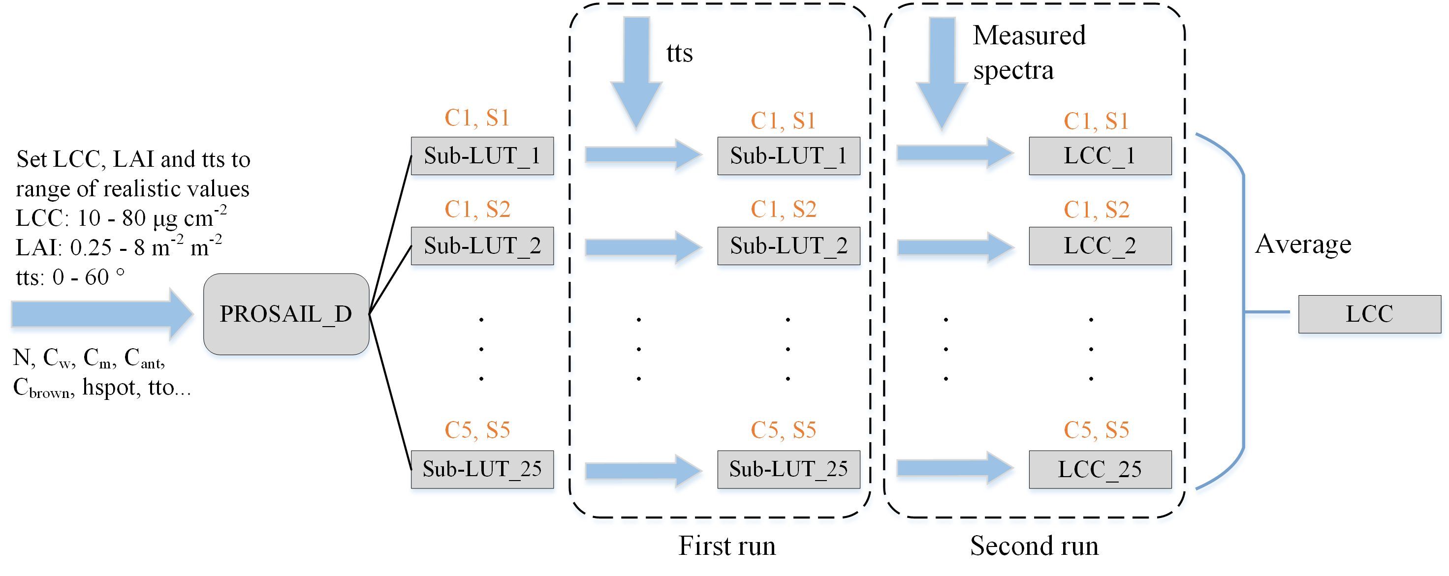
The field measurements were conducted at three sites (Figure 1). The first site is located at the National Precision Agriculture Demonstration Base in Xiaotangshan (XTS) town, Beijing, China. The size of the XTS is about 167 ha. Winter wheat, planted at this site, is considered one of the most important crops in China. In the 2002 campaign, the study area was divided into 48 small plots, each of which was 32.4 m × 30.0 m, separated by a 1-m wide isolation strip from adjacent plots. Four nitrogen fertilization treatments (0, 150, 300 and 450 kg ha⁻¹), four irrigation treatments (0, 225, 450 and 675 m³ ha⁻¹) and three winter wheat varieties (Jingdong 8, Zhongyou 9507 and Jing 9428) were used in these experiments. In the 2004 campaign, 21 winter wheat varieties were planted, including 7 relatively straight leaf type varieties, 7 relatively horizontal leaf type varieties and 7 common leaf type varieties. For each variety, there were two duplicate plots. All 42 plots were normally managed with the same fertilization and irrigation [49,50]. The other two sites (US-Ne2 and US-Ne3) are located at the University of Nebraska–Lincoln Agricultural Research and Development Center near Mead, Nebraska, USA. US-Ne2 is a 65-ha field equipped with a center-pivot irrigation system. US-Ne3 is about the same size, but depends entirely on rainfall to obtain moisture. US-Ne2 and US-Ne3 are both planted in a maize (odd years)–soybean (even years) rotation. Further detailed information is shown in

Table 1. Details of the study sites.

Sites	Latitude	Longitude	Crop Species	Field Measurement Dates
XTS	40°10′48′′ N	116°26′24′′ E	Wheat	04/02, 04/10, 04/18, 05/06, 05/17/2002 04/14, 04/21, 04/28, 05/11, 05/19/2004
US-Ne2	41°9′54′′ N	96°28′12″ W	Soybean	06/13–09/17/2002, 27 measurement campaigns 06/29–09/20/2004, 21 measurement campaigns
US-Ne3	41°10′47″ N	96°26′23″ W	Soybean	06/19–09/17/2002, 25 measurement campaigns

.

2.2. Canopy Reflectance Measurements

At the XTS site, a 1-m² area of wheat in each plot was selected for canopy spectral reflectance measurements using an ASD FieldSpec Pro spectrometer (Analytical Spectral Devices, Boulder, CO, USA) with spectral resolutions of 3 nm from 350 to 1050 nm and 10 nm from 1050 to 2500 nm. To ensure the accuracy of the data, the measurements were taken under clear weather conditions between 10:00 and 14:00 local time at nadir direction, approximately 1.3 m above the canopy, and with a 25° field of view. The averaged reflectance spectra were obtained for each plot by averaging the spectra acquired from 20 independent measurements [50].

At the US-Ne2 and US-Ne3 sites, canopy reflectance spectra measurements were performed between 11:00 and 13:00 local time using a hyperspectral radiometer mounted on “Goliath”, an all-terrain sensor platform [51]. Radiometric data with a spectral range of 400–1100 nm and a spectral resolution of 1.5 nm were acquired using a dual fiber-optic system that included two mutually calibrated Ocean Optics USB2000 radiometers. One of the radiometers pointed downwards to measure the upwelling radiance of the soybean at a height of about 5.5 m with a field of view of 25°. The other was equipped with a cosine diffuser to yield a hemispherical field of view and pointed upwards to measure the incident irradiance simultaneously. The canopy reflectance was then calculated based on the measured radiance and irradiance spectra (see [52] for details).

2.3. Leaf Chlorophyll Content Measurements

At the XTS site, after acquiring the canopy spectra, two fully unfolded leaves at the top of the canopy of all plants in four 60-cm-long rows per plot (with a row spacing of 15 cm) were harvested on each investigation date, placed in a black plastic bag under cool conditions to keep the leaves fresh and prevent moisture loss and transported to the laboratory for measurement of LCC. The LCC was obtained by standard laboratory spectrophotometry measurements [53]. First, samples of fresh wheat leaves were mixed with a given volume of 80% alcohol solution. Each sample was put in a cuvette and kept in darkness at 25 °C for 48 h. Next, an L6 ultraviolet-visible spectrophotometer was used to measure the pigment absorption at 663 and 646 nm. Then, the LCC could be calculated according to the absorbances of the extract solution at 663 and 646 nm. At the US-Ne2 and US-Ne3 sites, the leaves were punched and LCC was determined analytically. The leaf pigment was extracted with 80% acetone, from circular leaf punches with a diameter of 1 cm. The LCC was calculated using a Cary 100 Varian spectrophotometer and equations by Porra et al. [54]. The statistical analyses of the measured wheat and soybean LCC are shown in

Table 2. Summary statistics of the measured wheat and soybean LCC (μg cm⁻²).

Sites	Crop Species	Year	n	Mean	Min	Max	SD	CV
XTS	Wheat	2002	223	51.914	32.384	79.940	12.365	0.238
		2004	85	54.284	29.449	79.993	8.325	0.153
US-Ne2	Soybean	2002	27	31.361	20.319	44.961	7.601	0.242
		2004	21	37.924	12.058	64.876	14.469	0.382
US-Ne3	Soybean	2002	25	32.344	13.328	40.085	7.493	0.232

n, number of samples; Min, minimum value; Max, maximum value; SD, standard deviation; CV, coefficient of variation.

.

2.4. ENVISAT MERIS and Sentinel-3 OLCI Datasets

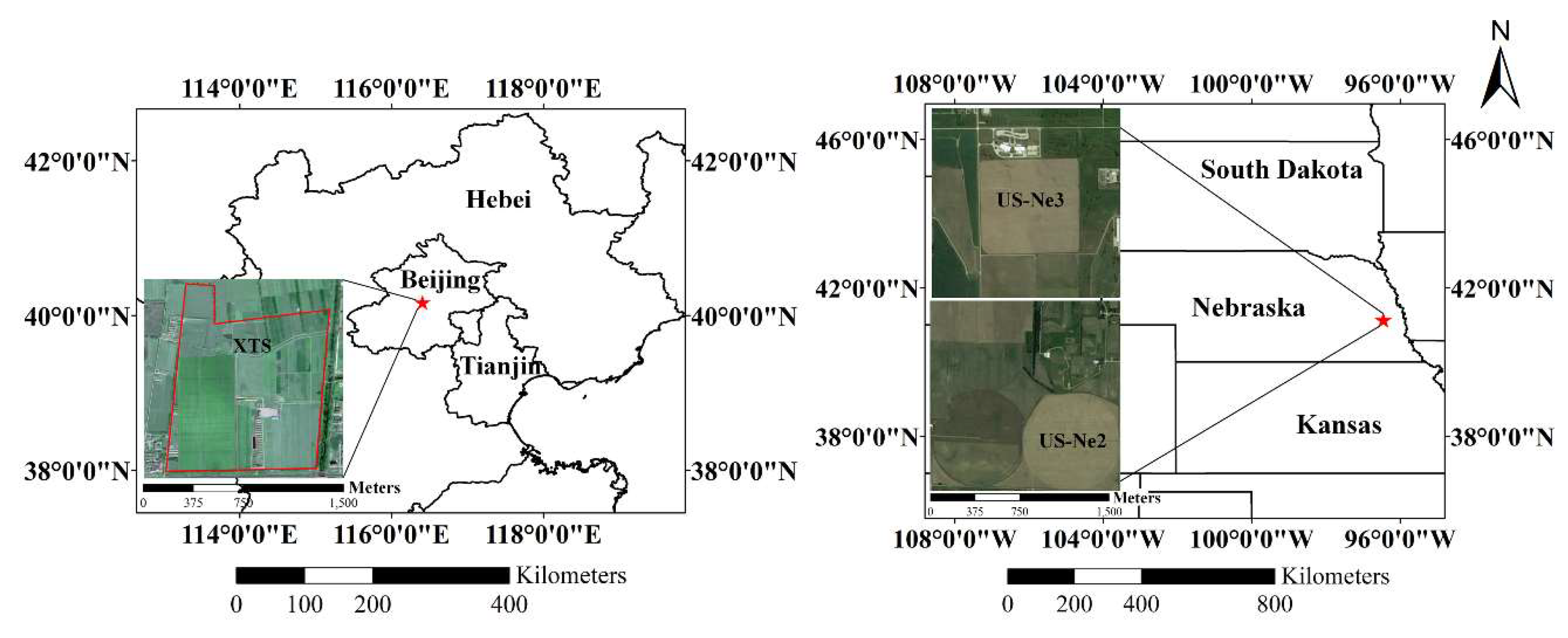
MERIS was one of the main instruments onboard the ENVISAT platform of the European Space Agency (ESA). MERIS data can be used to measure and monitor vegetation due to their high spectral resolution, medium spatial resolution and a 2–3-day revisit cycle. Full resolution, 7-day surface reflectance products for 2004 were acquired from the Climate Change Initiative—ESA. MERIS has 15 bands, spanning the visible to shortwave infrared with a spatial resolution of 300 m. Sentinel-3 is also an Earth observation satellite constellation launched by ESA. It currently consists of 2 satellites. Sentinel-3 OLCI, the successor to MERIS, has a resolution of 300 m and 21 wavebands, allowing global coverage in less than 4 days. MERIS and OLCI images covering the US-Ne2 study site are shown in Figure 2.

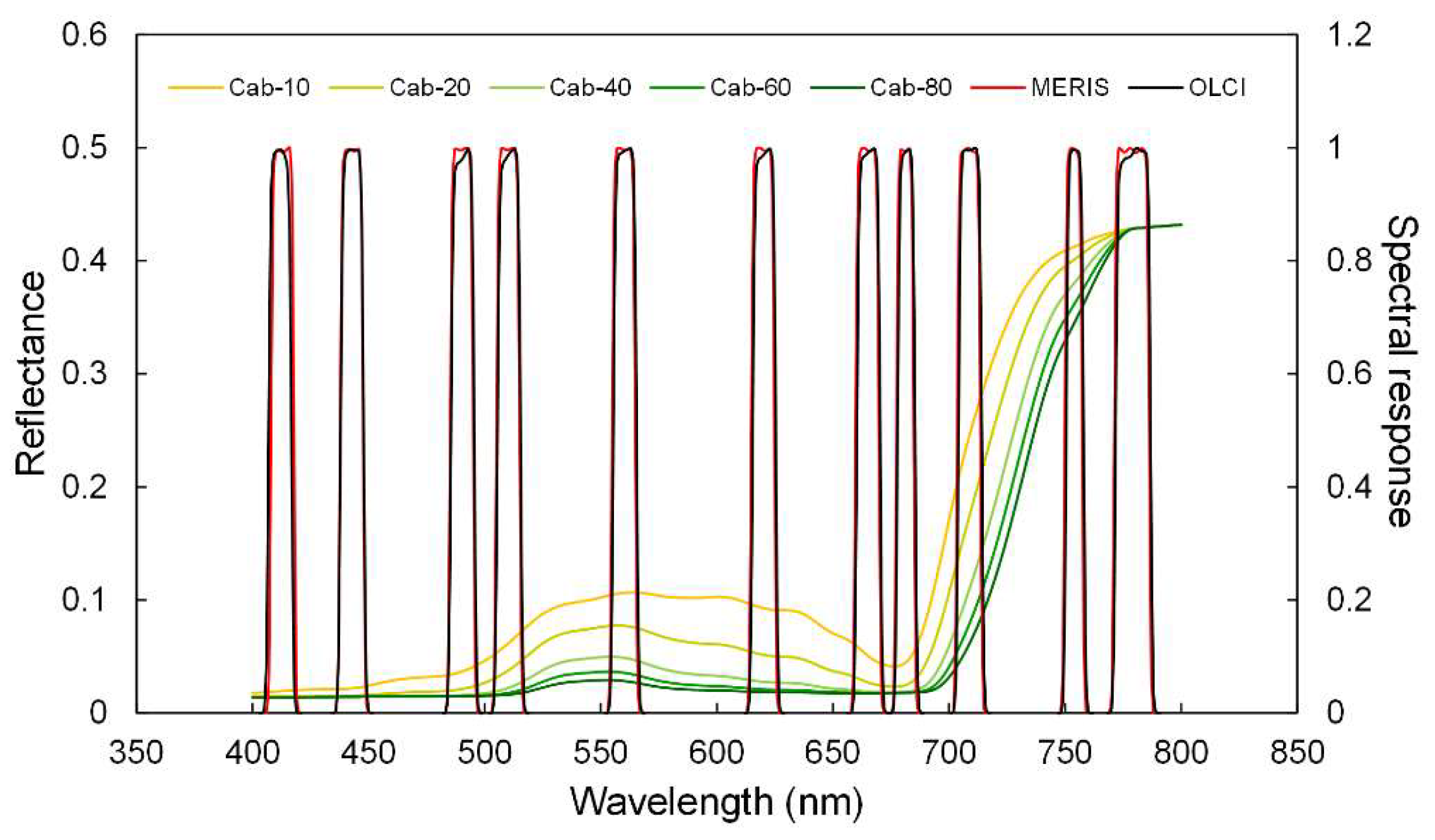
The two instruments have the same band settings and similar spectral response functions (

Table 3. Band specifications of the MERIS and OLCI used in this study.

MERIS	OLCI	Band Center (nm)	Band Width (nm)
B1	B2	412.5	10
B2	B3	442.5	10
B3	B4	490	10
B4	B5	510	10
B5	B6	560	10
B6	B7	620	10
B7	B8	665	10
B8	B10	681.25	7.5
B9	B11	708.75	10
B10	B12	753.75	7.5
B12	B16	778.75	15

and Figure 3). Therefore, the inversion methods developed for MERIS can generally be applied to OLCI datasets. All the MERIS bands except bands 11 (760.625 nm) and 15 (900 nm) (surface reflectance products lack bands 11 and 15) were used for analysis in this study. Since the red edge is the region most sensitive to chlorophyll content, different combinations of red-edge bands were selected to find the optimal combination.

2.5. MERIS and Sentinel-3 Red-Edge Indices

Several vegetation indices (VIs) sensitive to LCC were selected in this study (

Table 4. Vegetation indices used in this study.

Index	Formula	Reference
MTCI	$\frac{R_{753.75}-R_{708.75}}{R_{708.75}-R_{681.25}}$	Dash and Curran [60]
ND705	$\frac{R_{753.75}-R_{708.75}}{R_{753.75}+R_{708.75}}$	Gitelson and Merzlyak [56]
CIred-edge	$\frac{R_{778.75}}{R_{708.75}}-1$	Gitelson et al. [55]
CIgreen	$\frac{R_{778.75}}{R_{560}}-1$	Gitelson et al. [24]
TCARI/OSAVI	$\frac{3\left[\left(R_{708.75}-R_{665}\right)-0.2\times \left(R_{708.75}-R_{560}\right)\left(R_{708.75}/R_{665}\right)\right]}{\left(1+0.16\right)\left(R_{865}-R_{665}\right)/\left(R_{865}+R_{665}+0.16\right)}$	Haboudane et al. [59]
MCARI/OSAVI	$\frac{\left[\left(R_{708.75}-R_{665}\right)-0.2\times \left(R_{708.75}-R_{560}\right)\right]\left(R_{708.75}/R_{665}\right)}{\left(1+0.16\right)\left(R_{865}-R_{665}\right)/\left(R_{865}+R_{665}+0.16\right)}$	Haboudane et al. [59]

). Since the band settings were similar, we calculated the indices using the MERIS bands only as the results for MERIS and OLCI would be similar. Simple and normalized difference ratios were used: two chlorophyll indices based on simple ratios, i.e. CI_red-edge and CI_green [24,55], and the normalized difference ratio ND₇₀₅ [56]. These ratios were chosen because of their accurate prediction of LCC in previous studies [24,56,57]. Combined spectral indices, such as the Transformed Chlorophyll Absorption in Reflectance Index (TCARI) normalized by the Optimized Soil-Adjusted Vegetation Index (OSAVI) (TCARI/OSAVI) and the Modified Chlorophyll Absorption in Reflectance Index (MCARI) normalized by OSAVI (MCARI/OSAVI), were also selected [58,59]. A reflectance difference ratio, the MERIS Terrestrial Chlorophyll Index (MTCI) [60], was also used in this study. Empirical models that used these VIs were built and compared with the LUT-based LCC retrieval that is described below.

2.6. The PROSAIL-D Radiative Transfer Model

The PROSAIL-D model was used to simulate MERIS observations and to assess the LCC retrieval performance in this study. PROSAIL-D—a combination of the leaf model PROSPECT-D [61] and the canopy model SAIL [62]—is widely used for the retrieval of vegetation parameters [45,63,64,65,66]. The PROSPECT-D model has 7 input parameters, as shown in

Table 5. Specific parameters input to the PROSAIL-D model for generating simulated spectra and the LUTs.

Parameter	Description	Unit	Value/Source
Leaf optical properties model (PROSPECT-D)
N	Leaf structural parameter	—	1.5
LCC	Leaf chlorophyll content	μg cm−2	10–80, step 10
Car	Leaf carotenoid content	μg cm−2	25% LCC
Cw	Equivalent water thickness	cm	0.02
Cm	Dry matter content	g cm−2	0.004
CAnt	Leaf anthocyanin content	μg cm−2	2
Cbrown	Leaf brown pigment content	—	0
Canopy reflectance model (SAIL)
LIDFa, LIDFb	Average leaf inclination angle	—	[1,0], [0,−1], [0,1], [−0.35, 0.15], [0,0]
LAI	Leaf area index	m−2 m−2	0.25, 0.5, 0.75, 1, 1.25, 1.5, 1.75, 2, 3, 4, 5, 6, 7, 8
hspot	Hot spot parameter	m m−1	0.05
ρsoil	Soil reflectance	—	As shown in Figure 4
tts	Solar zenith angle	Deg	0, 10, 20, 30, 40, 50, 60
tto	View zenith angle	Deg	0
psi	Relative azimuth angle	Deg	0
skyl	Fraction of diffuse incoming solar radiation	—	According to incident light conditions

[1,0], planophile; [0,−1], plagiophile; [0,1], extremophile; [−0.35,−0.15], spherical; [0,0], uniform.

. The output parameters are the leaf spectral reflectance and transmittance. The SAIL model requires several parameters that describe the canopy structure, the soil background and observation-related variables, as well as the leaf spectral reflectance and transmittance to simulate the canopy reflectance.

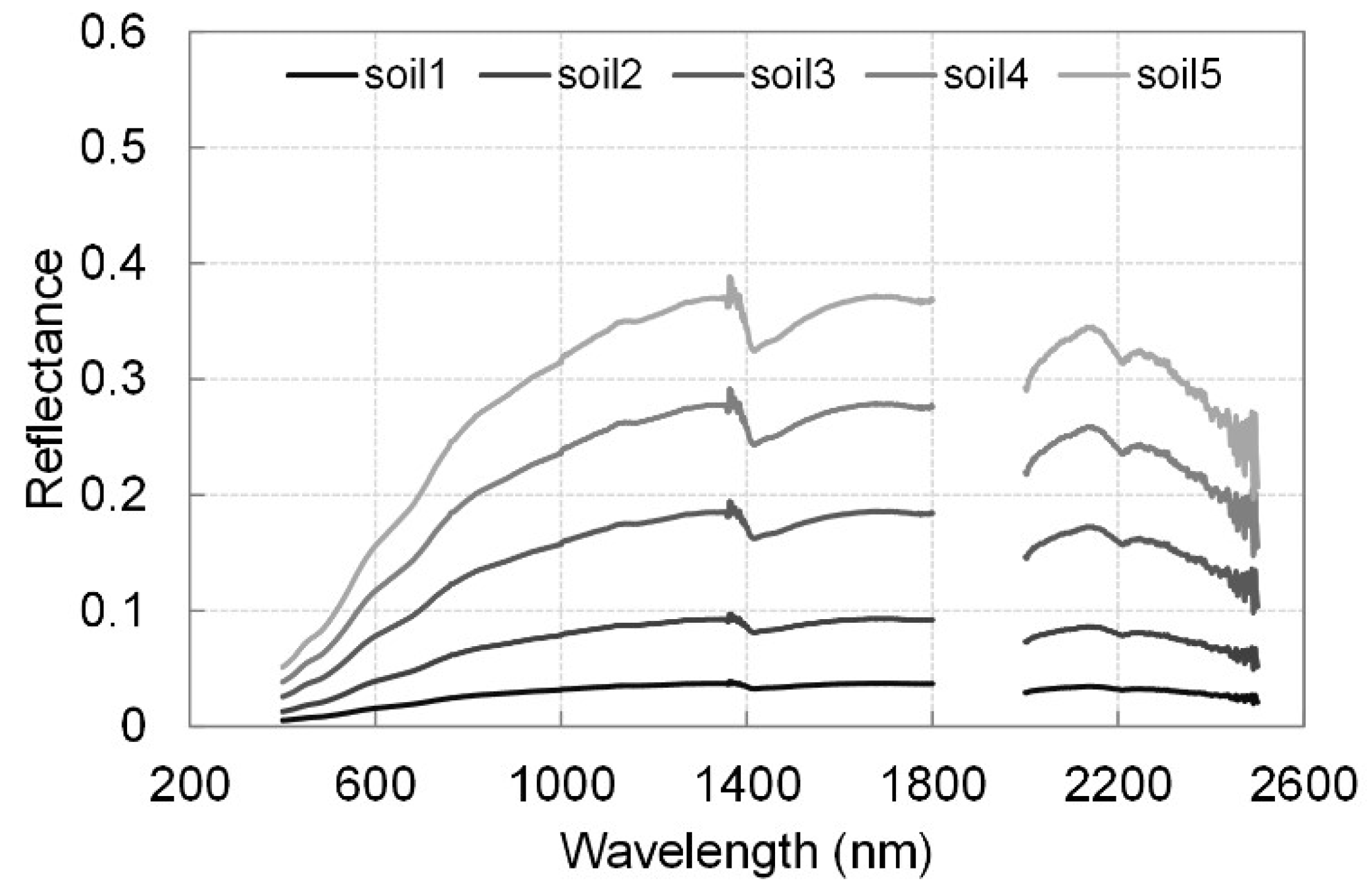
As shown in Table 5, in the simulation, the leaf carotenoid content was simply set to 25% of the LCC because it mainly affects the reflectance of the blue bands, which were not used to retrieve the LCC. Plants assumed to have an erectophile distribution were not considered because of the underestimation of the LCC, which causes a big error in the overall inversion results [47]. The values of LAI were ranged from 0.25 to 8, representing different levels of vegetation coverage. The soil backgrounds were simulated using the field-measured spectra of bare, dry soil multiplied by different brightness coefficients (Figure 4). The values of the solar zenith angle were set from 0° to 60°, with a step of 10°. The fraction of diffuse incoming solar radiation (skyl) was set to correspond to different incident light conditions. It should be noted that canopy spectra resampling was carried out to match the corresponding full width at half maximum (FWHM) and central wavelengths of the MERIS and OLCI bands used for retrieving LCC from the simulated dataset.

2.7. Model Inversion

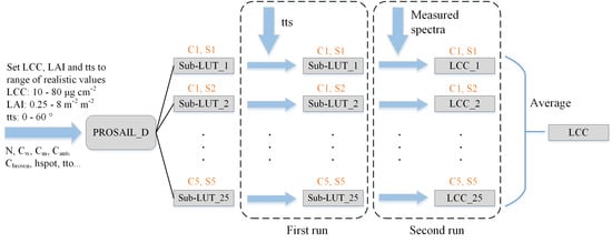
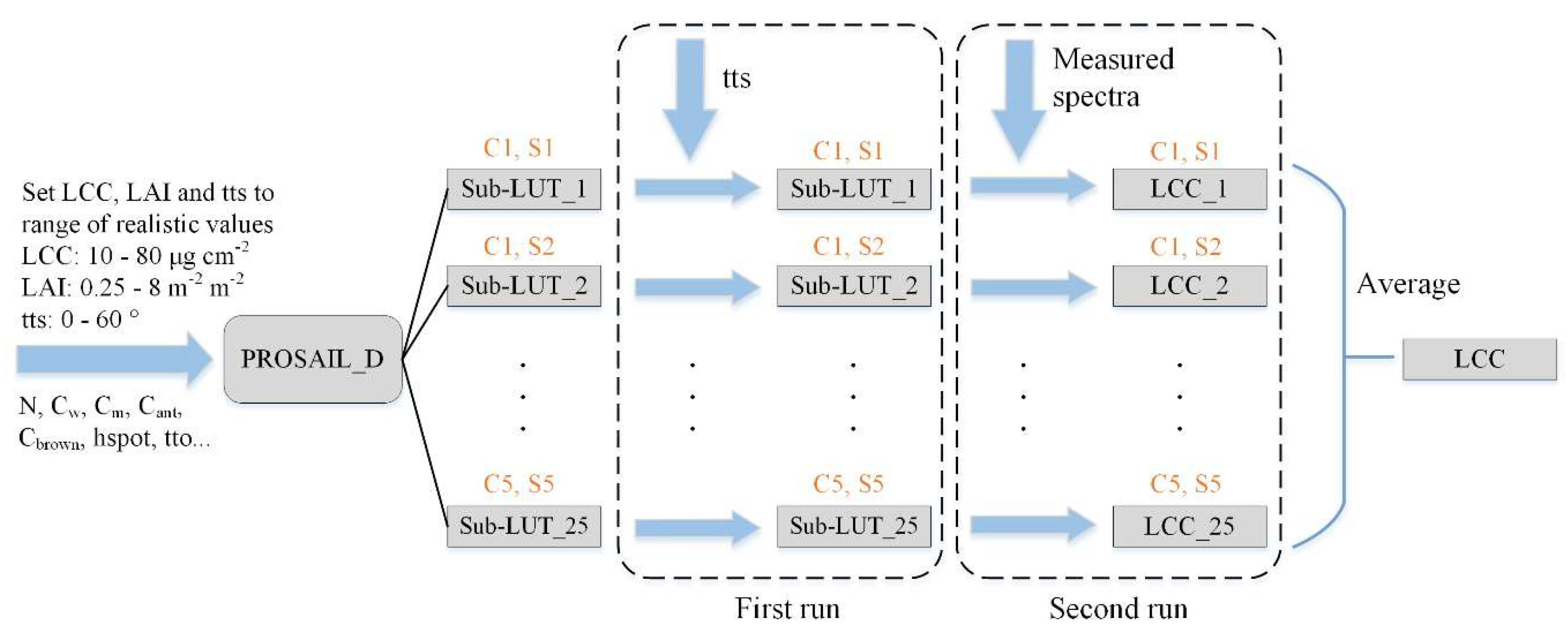
As shown in Figure 5, a LUT that included 25 sub-LUTs corresponding to 5 types of canopy structure and 5 types of soil background was generated. To further deal with the ill-posed problem and to improve the LCC inversion accuracy, we used the prior knowledge of solar zenith angle that can be calculated according to the measurement date to generate a second group of 25 sub-LUTs. To find the estimated value of the inversion, the RMSE for the sub-LUT was calculated using

$$\mathrm{RMSE}=\sqrt{\frac{{{\displaystyle \sum }}_{\mathrm{i}=1}^{\mathrm{n}}{\left({\mathrm{R}}_{\mathrm{measured}}\left({\mathsf{\lambda }}_{\mathrm{i}}\right)-{\mathrm{R}}_{\mathrm{simulated}}\left({\mathsf{\lambda }}_{\mathrm{i}}\right)\right)}^2}{\mathrm{n}}}$$

(1)

where n is the number of wavebands used in the retrieval, ${\mathrm{R}}_{\mathrm{measured}}$ is the measured reflectance, ${\mathrm{R}}_{\mathrm{simulated}}$ is the simulated reflectance and $\mathsf{\lambda }$ is the corresponding spectral band. In the traditional inversion process, the single solution with the smallest RMSE value would be used as the inversion result. However, in this study, except for the single solution obtained for the smallest RMSE value, the means of the best 3, 5, 8, 10 and 15 solutions were also examined in each sub-LUT. For example, the best 3 solutions refer to the 3 chlorophyll inversion values corresponding to the first 3 smallest RMSE values in the process of inverting the LCC in each sub-LUT. It was found that the mean of the best 8 solutions produced the lowest RMSE for the LCC retrieval. Therefore, instead of the single best solution with the smallest RMSE value, the mean of the best 8 solutions was selected as the retrieval of each sub-LUT. By combining multiple types of canopy structure and soil background, the final inversion result was the one obtained by averaging the retrievals of the 25 sub-LUTs. Multiple averages will reduce the ill-posed inversion problem, improve the robustness of the inversion method, and thus improve the applicability to different canopy structures and soil backgrounds.

In addition, inversion results based on different inversion strategies, such as considering one canopy structure with five types of soil background and one type of soil background with five types of canopy structure, were also assessed. For convenience, the method in which the inversion results for five different canopy structures and five different soil backgrounds were averaged is labeled here as M-M.

3. Results

3.1. LCC Estimation Using the Simulated Dataset

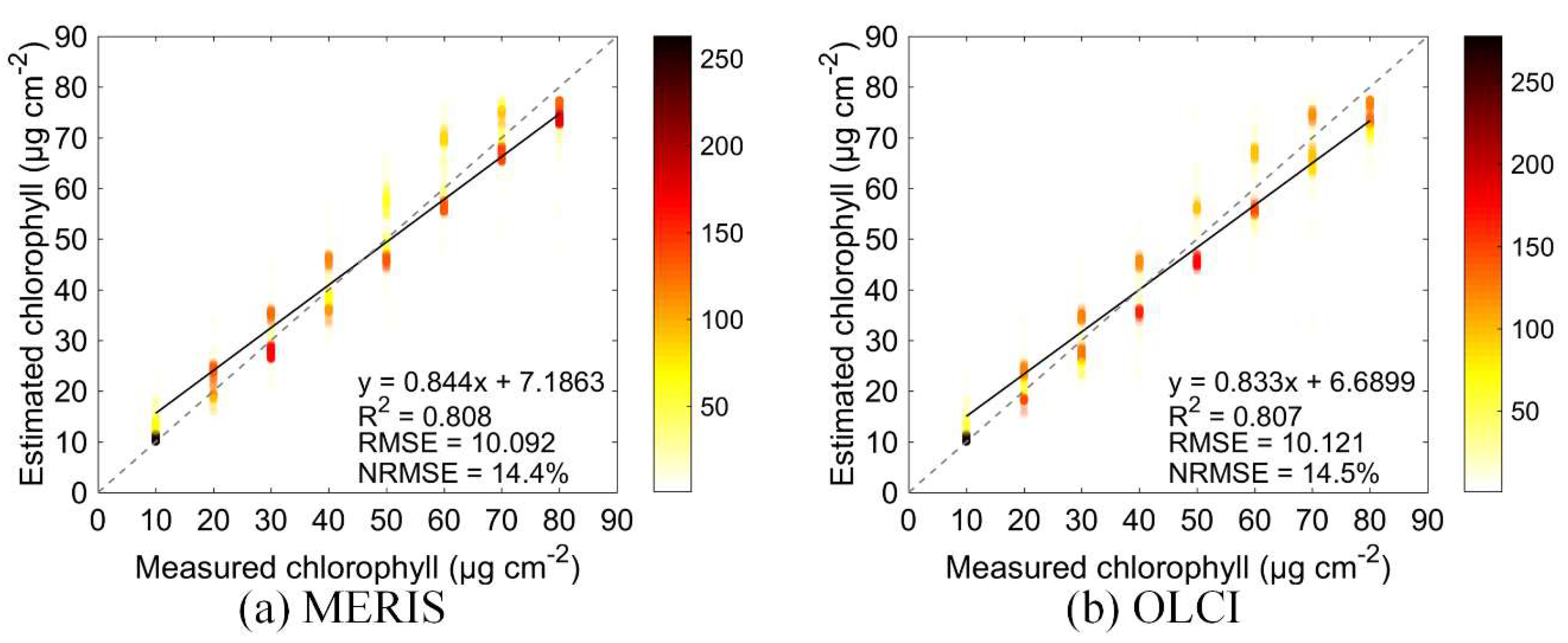
The determination coefficient (R²), RMSE and normalized RMSE (NRMSE = RMSE/range) values were selected to assess the inversion accuracy obtained using the LUT approach with the simulated dataset. Figure 6 exhibits the relationships between the measured LCC and that estimated using the LUT approach (R² = 0.81, RMSE = 10.1 μg cm⁻² for MERIS; and R² = 0.81, RMSE = 10.1 μg cm⁻² for OLCI).

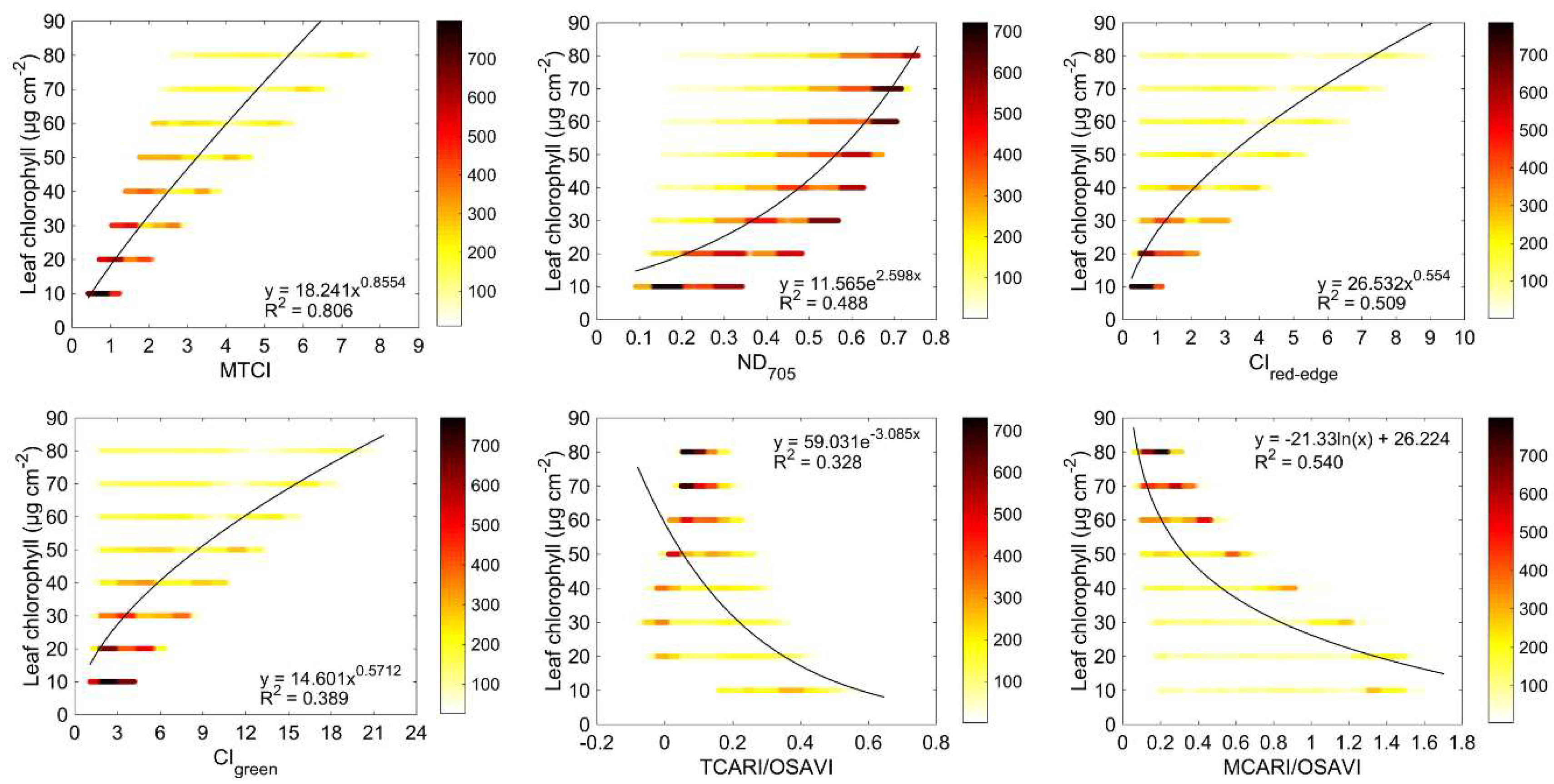
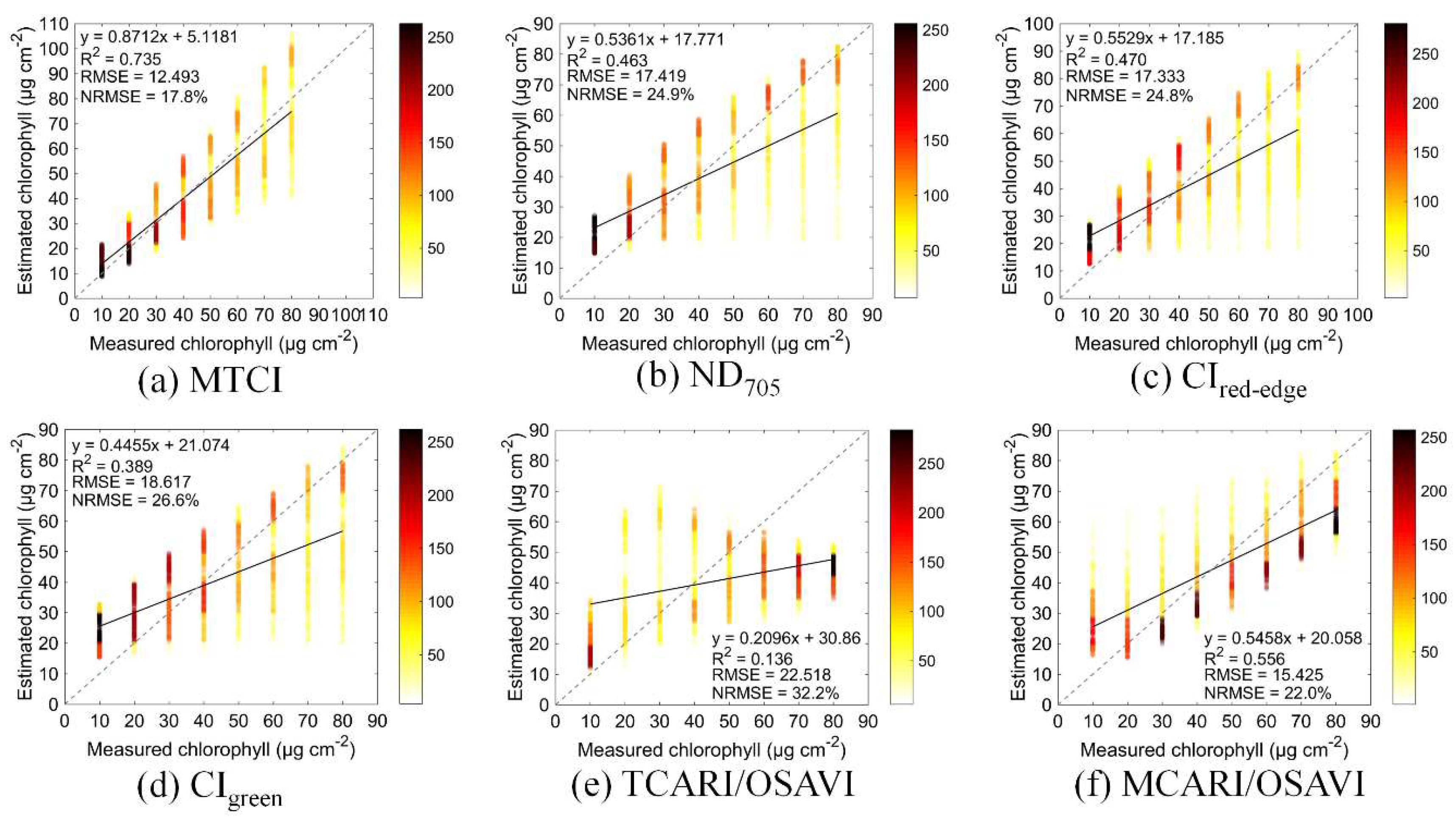
For comparison, the LCC was also estimated using the selected VIs. First, empirical regression models between the LCC and the VIs were established using the simulated dataset. For each VI, the strongest regression relationship among the linear, polynomial, power, logarithmic and exponential relationships was then chosen. As shown in Figure 7, MTCI exhibited the highest R² value (0.81), followed by MCARI/OSAVI (R² = 0.54) and CI_red-edge (R² = 0.51). Unexpectedly, ND₇₀₅, CI_green and TCARI/OSAVI did not perform well in this study, producing R² values lower than 0.5. Figure 8 shows the inversion performance obtained using the VI approach for the validation dataset. Consistent with the modeling results, the MTCI vegetation index yielded the highest prediction accuracy, giving the highest R² (0.74), the lowest RMSE (12.5 μg cm⁻²) and NRMSE values (17.8%). The LCC inversion results suggested that the LUT approach had the greatest potential to retrieve LCC using the simulated dataset. Because of the low inversion accuracy of the other VIs, only the MTCI was adopted for comparison with the LUT approach in terms of the retrieval of the LCC using field-measured canopy spectra and satellite data.

3.2. LCC Estimation Using Field-Canopy Reflectance Measurements

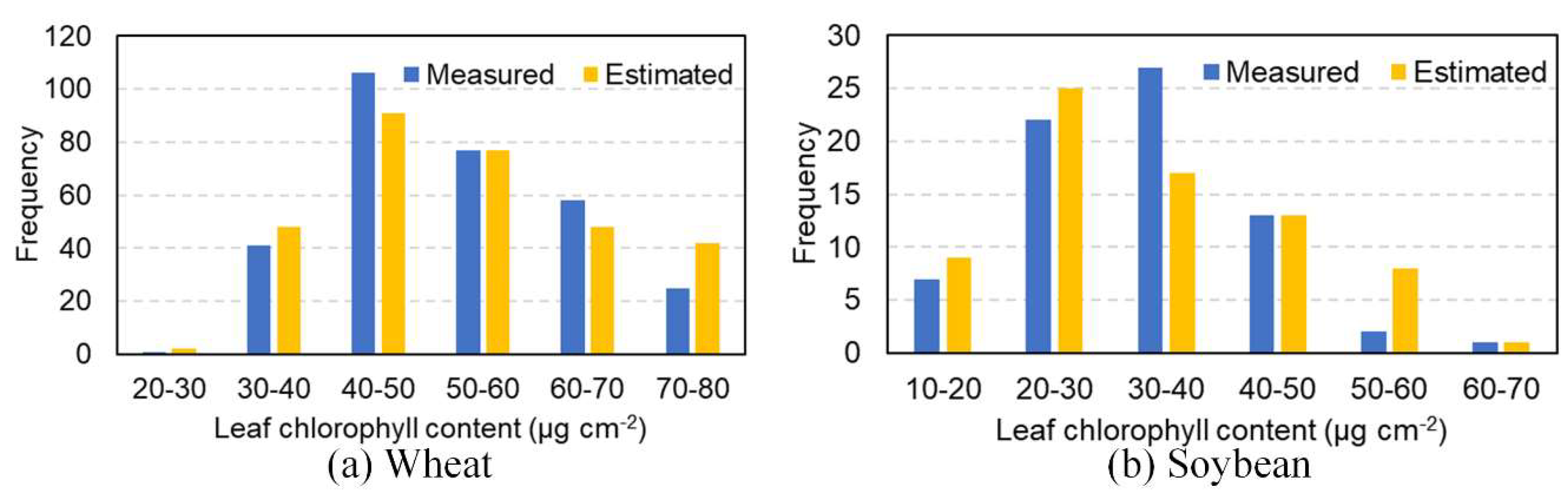
Field-measured canopy spectra convolved with the MERIS spectral response function were used to simulate the MERIS band reflectance. As shown in Figure 9a,c, both for wheat and soybean, the regression lines were close to the 1:1 line, with an RMSE value lower than 10 μg cm⁻². For comparison, the LCC was also retrieved using the MTCI. The inversion results produced a large overestimate of the LCC for both wheat and soybean. Furthermore, even when the data for wheat and soybean were put together, they still produced a good inversion accuracy (Figure 9e). As shown in Figure 10, the overall distribution of the measured and estimated LCC histogram was similar. Although the results in Figure 9 show that the inversion accuracy of soybean LCC was slightly higher than that of wheat, from the perspective of numerical distribution, the distribution of wheat LCC estimates was closer to the measured values. These results indicate that the LUT approach yielded great potential for estimating the LCC using field-measured canopy spectra of wheat and soybean.

3.3. LCC Estimation Using MERIS Satellite Data

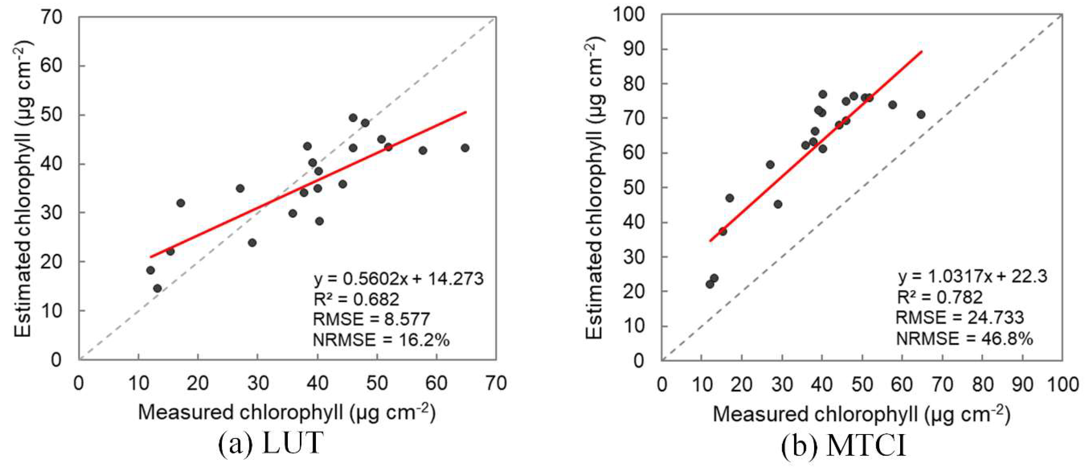
For the verification of the method using real satellite data, the dataset from US-Ne2 acquired in 2004 was selected because it was aligned with the MERIS acquisitions. In contrast, the dataset acquired at the XTS site lacked a sufficiently long time series. Thus, data from the XTS site were not used for verification at this scale. The relationship between the measured LCC and that estimated using the LUT approach is shown in Figure 11a. The improved LUT method yielded reasonable results, with an R² value of 0.68 and an RMSE value of 8.6 μg cm⁻². The estimation performance achieved using the MTCI was also examined, and the results show that this method produced an overestimate. These results suggest that, using MERIS satellite data, the LUT approach performed better LCC retrievals than the MTCI-based approach.

4. Discussion

It has already been stated that parameter retrieval methods using LUTs are ill-posed because different combinations of canopy and leaf parameters may produce similar spectra [67,68]. Prior knowledge is very useful for constraining parameters. However, the specific local circumstances limit its applicability to larger scales and other areas. For instance, in previous studies, the canopy structure has been assumed to be ellipsoidal for specific crops [47,69]. Such an assumption is reasonable under specific conditions but cannot be applied at large scales. In our study, the leaf biochemical parameters which influence the bands of the canopy spectra that are insensitive to LCC were also constrained. In contrast, we selected relatively wide ranges of values and types for the LCC, LAI, canopy structure and soil background. A main LUT, covering different types of canopy structure and soil background that represent the expected ranges of typical crop conditions, was used. In the inversion process, firstly the eight best inversion results of each sub-LUT were averaged, and then the mean value of the LCC inversion result of 25 sub-LUTs was considered as the retrieval. Multiple averages will improve the robustness of the inversion method, and thus improve the applicability to different canopy structures and soil backgrounds. The inversion results of all canopy types and soil backgrounds were averaged to reduce the inversion deviation caused by uncertainty.

4.1. LCC Retrieval Performance Using Different Combinations of MERIS Bands

It is well known that using only a selection of spectral bands may yield a better inversion accuracy than using all the bands. Consequently, the selection and performance of specific bands are critical for an accurate LCC inversion using the LUT method. Here, we assessed the potential of LCC retrieval using different combinations of MERIS bands. As shown in

Table 6. Comparisons of LCC retrieval performance using different combinations of MERIS bands.

Combination	Bands Used	PROSAIL Simulation		Measured Wheat		Measured Soybean		MERIS Soybean
		R2	RMSE (μg cm−2)	R2	RMSE (μg cm−2)	R2	RMSE (μg cm−2)	R2	RMSE (μg cm−2)
G1	band 1–10, 12–14	0.763	11.811	0.401	8.996	0.334	11.708	0.343	11.562
G2	band 1–10, 12	0.772	11.282	0.416	9.149	0.341	11.498	0.393	11.282
G3	band 7–10	0.773	11.112	0.405	10.709	0.339	12.162	0.509	10.316
G4	band 7–9	0.808	10.092	0.437	9.859	0.452	9.578	0.682	8.577
G5	band 7, 8, 10	0.361	18.324	0.366	11.025	0.061	14.275	0.089	15.213
G6	band 7, 9, 10	0.783	10.887	0.413	10.830	0.343	12.218	0.517	10.442
G7	band 8–10	0.785	10.863	0.415	10.843	0.340	12.207	0.522	10.467
G8	band 8, 9, 12	0.797	10.791	0.404	10.424	0.434	12.321	0.578	10.520

PROSAIL simulation represents that the data used were the simulation spectra convolved with the MERIS spectral response function. Measured wheat represents that the data used were the field-measured wheat canopy spectra convolved with the MERIS spectral response function. Measured soybean represents that the data used were the field-measured soybean canopy spectra convolved with the MERIS spectral response function. MERIS soybean represents that the data used were the soybean canopy spectra from the MERIS satellite.

, first, all bands were selected, which resulted in RMSE values greater than 11 μg cm⁻², except for the wheat site. When only red-edge bands were used, it can be seen from a comparison between the G4 and G5 combinations that there was a large decrease in the inversion accuracy when band 9 was replaced by band 10, indicating that band 9 plays a pivotal role in the retrieval of LCC from MERIS data. Surprisingly, the addition of near-infrared band information did not improve the inversion accuracy of LCC even though the near-infrared bands are sensitive to LAI. In addition, the different combinations of VIs listed in Table 4 were also tested, but the results were not as accurate as those obtained using red-edge band reflectance (these results are not shown). Therefore, it may be concluded that the retrieval of LCC using red-edge band reflectance outperforms that using the VIs sensitive to LCC. The results also demonstrate that the combination of bands 7 (665 nm), 8 (681.25 nm) and 9 (708.75 nm) is the optimal combination for LCC retrieval from MERIS and OLCI data.

4.2. LCC Retrieval Performance Using Different Inversion Strategies

To quantify that the inversion strategy combining multiple types of canopy structure and soil background can improve the inversion accuracy, the retrieval of LCC from both field canopy spectra and MERIS satellite data using different strategies was compared. M-M represents the method in which the inversion results for five types of canopy structure and five types of soil background were averaged. As shown in

Table 7. Comparisons of LCC retrieval performance using different inversion strategies. The results in bold are the results obtained using the inversion strategy proposed in this study.

Strategy	Measured Wheat		Measured Soybean		MERIS Soybean
	R2	RMSE (μg cm−2)	R2	RMSE (μg cm−2)	R2	RMSE (μg cm−2)
M-M	0.437	9.859	0.452	9.578	0.682	8.577
M-C1	0.426	10.540	0.421	9.739	0.670	10.194
M-C2	0.433	10.385	0.457	10.113	0.679	8.212
M-C3	0.432	10.881	0.463	10.709	0.651	8.382
M-C4	0.428	10.722	0.427	9.752	0.687	10.335
M-C5	0.435	10.654	0.463	10.396	0.680	8.075
M-S1	0.309	23.088	0.428	13.875	0.381	21.251
M-S2	0.396	19.954	0.412	13.963	0.377	20.338
M-S3	0.451	12.504	0.411	13.035	0.597	9.737
M-S4	0.411	15.493	0.348	12.960	0.600	13.498
M-S5	0.391	17.582	0.269	16.098	0.652	18.528

M-M represents the method in which the inversion results for five types of canopy structure and five types of soil background were averaged. M-C1–M-C5 represent the methods in which the inversion results only for the canopy structure planophile, plagiophile, extremophile, spherical and uniform were averaged, respectively. M-S1–M-S5 represent the methods in which the inversion results only for the soil backgrounds soil1, soil2, soil3, soil4 and soil5 were averaged, respectively.

, for wheat, M-M had the lowest RMSE value. Among the inversion results obtained for different soil backgrounds, the R² value for M-M was second only to M-S3 and the RMSE value was the lowest. Comparing the results for the inversion of soybean LCC using field canopy spectra, the RMSE value of M-M was also found to be the lowest. Finally, the inversion results using satellite data illustrated that the M-M combination did not differ much from the best results. Therefore, it can be concluded that the use of the LUT approach combining multiple canopy structures and soil backgrounds has great potential for estimating LCC, although the inversion accuracy is likely to be better if the canopy structure is known. Moreover, the difference in inversion accuracy may be acceptable when the difficulty of obtaining information about canopy structure and soil background over large areas is taken into consideration.

Although MEIRS is no longer in operation, it is helpful to produce products with long time series. This study did not consider the clumping effect. Such effect is relatively small for crops, while, for other vegetation types, such as forests, the clumping effect would have a larger impact. Therefore, future work will consider LUTs created by 3D radiative transfer models such as 4-Scale or DART to test these methods over more species and regions, evaluating their accuracy and robustness.

5. Conclusions

Leaf chlorophyll content is a significant indicator for monitoring plant physiological status. In this study, we proposed an improved LUT approach to retrieving LCC through the inversion of the PROSAIL-D model by combining multiple canopy structures and soil backgrounds. The inversion results demonstrate that, using an LUT approach, the use of the red-edge bands produced better estimates of LCC than the use of red-edge vegetation indices alone. First, the LCC estimation results for a simulated dataset built with simulated spectra showed that the use of the LUT approach with MERIS/OLCI spectral bands had good potential for estimating LCC and produced an R² value of 0.81 and RMSE value of 10.1 μg cm⁻² for MERIS and an R² value of 0.81 and RMSE value of 10.1 μg cm⁻² for OLCI. Next, further validation of the proposed approach was carried out using field-measured canopy spectra and MERIS satellite data to retrieve LCC. This yielded an RMSE of 9.9 μg cm⁻² for wheat and 9.6 μg cm⁻² for soybean using canopy spectra simulating MERIS bandsets; for soybean, using MERIS data, the RMSE was 8.6 μg cm⁻². Furthermore, an empirical method using red-edge vegetation indices and a physical method using the PROSAIL-D model were compared. The results indicate that the LUT approach using MERIS bandsets provided accurate and robust estimates of LCC. These results demonstrate the feasibility of LCC estimation using the physical model inversion method from MERIS, as well as its applicability to Sentinel-3 OLCI satellite sensor for large monitoring of chlorophyll content in crops. The improved LUT approach to retrieving LCC proposed in this study could reduce the ill-posed inversion problem caused by the lack of prior knowledge on canopy structure and soil background, improve the robustness of the inversion method, and, consequently, improve the accuracy of LCC retrieval.

References

- Porcar-Castell, A.; Tyystjärvi, E.; Atherton, J.; Van der Tol, C.; Flexas, J.; Pfündel, E.E.; Moreno, J.; Frankenberg, C.; Berry, J.A. Linking chlorophyll a fluorescence to photosynthesis for remote sensing applications: Mechanisms and challenges. J. Exp. Bot. 2014, 65, 4065–4095. [Google Scholar] [CrossRef] [PubMed]
- Demmig-Adams, B.; Adams Iii, W.W. Photoprotection and other responses of plants to high light stress. Annu. Rev. Plant Physiol. Plant Mol. Biol. 1992, 43, 599–626. [Google Scholar] [CrossRef]
- Croft, H.; Chen, J.M.; Luo, X.; Bartlett, P.; Chen, B.; Staebler, R.M. Leaf chlorophyll content as a proxy for leaf photosynthetic capacity. Global Chang. Biol. 2017, 23. [Google Scholar] [CrossRef] [PubMed]
- Qian, X.; Zhang, Y.; Liu, L.; Du, S. Exploring the potential of leaf reflectance spectra for retrieving the leaf maximum carboxylation rate. Int. J. Remote Sens. 2019, 40, 5411–5428. [Google Scholar] [CrossRef]
- Inoue, Y.; Guérif, M.; Baret, F.; Skidmore, A.; Gitelson, A.; Schlerf, M.; Darvishzadeh, R.; Olioso, A. Simple and robust methods for remote sensing of canopy chlorophyll content: A comparative analysis of hyperspectral data for different types of vegetation. Plant Cell Environ. 2016, 39, 2609–2623. [Google Scholar] [CrossRef] [Green Version]
- Osborne, B.A. Light absorption by plants and its implications for photosynthesis. Biol. Rev. 1986, 61, 1–60. [Google Scholar] [CrossRef]
- Curran, P.J.; Dungan, J.L.; Gholz, H.L. Exploring the relationship between reflectance red edge and chlorophyll content in slash pine. Tree Physiol. 1990, 7, 33–48. [Google Scholar] [CrossRef]
- Clevers, J.G.P.W.; Kooistra, L.; Van den Brande, M.M.M. Using Sentinel-2 data for retrieving LAI and leaf and canopy chlorophyll content of a potato crop. Remote Sens. 2017, 9, 405. [Google Scholar] [CrossRef] [Green Version]
- Carter, G.A. Ratios of leaf reflectances in narrow wavebands as indicators of plant stress. Int. J. Remote Sens. 1994, 15, 697–703. [Google Scholar] [CrossRef]
- Gitelson, A.A.; Merzlyak, M.N. Remote estimation of chlorophyll content in higher plant leaves. Int. J. Remote Sens. 1997, 18, 2691–2697. [Google Scholar] [CrossRef]
- Houborg, R.; Anderson, M.C.; Daughtry, C.S.T.; Kustas, W.P.; Rodell, M. Using leaf chlorophyll to parameterize light-use-efficiency within a thermal-based carbon, water and energy exchange model. Remote Sens. Environ. 2011, 115, 1694–1705. [Google Scholar] [CrossRef]
- Meggio, F.; Zarco-Tejada, P.J.; Núñez, L.C.; Sepulcre-Cantó, G.; González, M.R.; Martín, P. Grape quality assessment in vineyards affected by iron deficiency chlorosis using narrow-band physiological remote sensing indices. Remote Sens. Environ. 2010, 114, 1968–1986. [Google Scholar] [CrossRef] [Green Version]
- Sampson, P.H.; Zarco-Tejada, P.J.; Mohammed, G.H.; Miller, J.R.; Noland, T.L. Hyperspectral remote sensing of forest condition: Estimating chlorophyll content in tolerant hardwoods. For. Sci. 2003, 49, 381–391. [Google Scholar] [CrossRef]
- Zhang, K.; Ge, X.; Shen, P.; Li, W.; Liu, X.; Cao, Q.; Zhu, Y.; Cao, W.; Tian, Y. Predicting rice grain yield based on dynamic changes in vegetation indexes during early to mid-growth stages. Remote Sens. 2019, 11, 387. [Google Scholar] [CrossRef] [Green Version]
- Zhang, K.; Liu, X.; Ma, Y.; Zhang, R.; Cao, Q.; Zhu, Y.; Cao, W.; Tian, Y. A comparative assessment of measures of leaf nitrogen in rice using two leaf-clip meters. Sensors 2020, 20, 175. [Google Scholar] [CrossRef] [Green Version]
- Luo, X.; Croft, H.; Chen, J.M.; He, L.; Keenan, T.F. Improved estimates of global terrestrial photosynthesis using information on leaf chlorophyll content. Global Chang. Biol. 2019, 25, 2499–2514. [Google Scholar] [CrossRef] [Green Version]
- Houborg, R.; Fisher, J.B.; Skidmore, A.K. Advances in remote sensing of vegetation function and traits. Int. J. Appl. Earth Obs. 2015, 43, 1–6. [Google Scholar] [CrossRef] [Green Version]
- Houborg, R.; Cescatti, A.; Migliavacca, M.; Kustas, W.P. Satellite retrievals of leaf chlorophyll and photosynthetic capacity for improved modeling of GPP. Agric. For. Meteorol. 2013, 177, 10–23. [Google Scholar] [CrossRef]
- Blackburn, G.A. Hyperspectral remote sensing of plant pigments. J. Exp. Bot. 2006, 58, 855–867. [Google Scholar] [CrossRef] [Green Version]
- Lichtenthaler, H.K.; Wellburn, A.R. Determinations of total carotenoids and chlorophylls a and b of leaf extracts in different solvents. Biochem. Soc. Trans. 1983, 603, 591–592. [Google Scholar] [CrossRef] [Green Version]
- Clevers, J.G.P.W.; Gitelson, A.A. Remote estimation of crop and grass chlorophyll and nitrogen content using red-edge bands on Sentinel-2 and -3. Int. J. Appl. Earth Obs. 2013, 23, 344–351. [Google Scholar] [CrossRef]
- Datt, B. Visible/near infrared reflectance and chlorophyll content in Eucalyptus leaves. Int. J. Remote Sens. 1999, 20, 2741–2759. [Google Scholar] [CrossRef]
- Maccioni, A.; Agati, G.; Mazzinghi, P. New vegetation indices for remote measurement of chlorophylls based on leaf directional reflectance spectra. J. Photochem. Photobiol. B Biol. 2001, 61, 52–61. [Google Scholar] [CrossRef]
- Gitelson, A.A.; Gritz, Y.; Merzlyak, M.N. Relationships between leaf chlorophyll content and spectral reflectance and algorithms for non-destructive chlorophyll assessment in higher plant leaves. J. Plant Physiol. 2003, 160, 271–282. [Google Scholar] [CrossRef] [PubMed]
- Curran, P.J. Remote sensing of foliar chemistry. Remote Sens. Environ. 1989, 30, 271–278. [Google Scholar] [CrossRef]
- Dawson, T.P.; Curran, P.J.; North, P.R.J.; Plummer, S.E. The Propagation of Foliar Biochemical Absorption Features in Forest Canopy Reflectance: A Theoretical Analysis. Remote Sens. Environ. 1999, 67, 147–159. [Google Scholar] [CrossRef]
- Li, D.; Tian, L.; Wan, Z.; Jia, M.; Yao, X.; Tian, Y.; Zhu, Y.; Cao, W.; Cheng, T. Assessment of unified models for estimating leaf chlorophyll content across directional-hemispherical reflectance and bidirectional reflectance spectra. Remote Sens. Environ. 2019, 231, 111240. [Google Scholar] [CrossRef]
- Le Maire, G.; François, C.; Soudani, K.; Berveiller, D.; Pontailler, J.Y.; Bréda, N.; Genet, H.; Davi, H.; Dufrêne, E. Calibration and validation of hyperspectral indices for the estimation of broadleaved forest leaf chlorophyll content, leaf mass per area, leaf area index and leaf canopy biomass. Remote Sens. Environ. 2008, 112, 3846–3864. [Google Scholar] [CrossRef]
- Wu, C.; Niu, Z.; Tang, Q.; Huang, W. Estimating chlorophyll content from hyperspectral vegetation indices: Modeling and validation. Agric. For. Meteorol. 2008, 148, 1230–1241. [Google Scholar] [CrossRef]
- Croft, H.; Chen, J.M.; Zhang, Y. The applicability of empirical vegetation indices for determining leaf chlorophyll content over different leaf and canopy structures. Ecol. Complex. 2014, 17, 119–130. [Google Scholar] [CrossRef]
- Liang, L.; Qin, Z.; Zhao, S.; Di, L.; Zhang, C.; Deng, M.; Lin, H.; Zhang, L.; Wang, L.; Liu, Z. Estimating crop chlorophyll content with hyperspectral vegetation indices and the hybrid inversion method. Int. J. Remote Sens. 2016, 37, 2923–2949. [Google Scholar] [CrossRef]
- Chemura, A.; Mutanga, O.; Odindi, J. Empirical modeling of leaf chlorophyll content in coffee (coffea arabica) plantations with sentinel-2 msi data: Effects of spectral settings, spatial resolution, and crop canopy cover. IEEE J. Sel. Topics Appl. Earth Observ. Remote Sens. 2017, 10, 5541–5550. [Google Scholar] [CrossRef]
- Sonobe, R.; Sano, T.; Horie, H. Using spectral reflectance to estimate leaf chlorophyll content of tea with shading treatments. Biosys. Eng. 2018, 175, 168–182. [Google Scholar] [CrossRef]
- Verrelst, J.; Muñoz, J.; Alonso, L.; Delegido, J.; Rivera, J.P.; Camps-Valls, G.; Moreno, J. Machine learning regression algorithms for biophysical parameter retrieval: Opportunities for Sentinel-2 and-3. Remote Sens. Environ. 2012, 118, 127–139. [Google Scholar] [CrossRef]
- Croft, H.; Chen, J.M. Leaf Pigment Content; Elsevier: Amsterdam, The Netherlands, 2017. [Google Scholar]
- Demarez, V.; Gastellu-Etchegorry, J.P. A modeling approach for studying forest chlorophyll content. Remote Sens. Environ. 2000, 71, 226–238. [Google Scholar] [CrossRef]
- Darvishzadeh, R.; Skidmore, A.; Abdullah, H.; Cherenet, E.; Ali, A.; Wang, T.; Nieuwenhuis, W.; Heurich, M.; Vrieling, A.; O’Connor, B. Mapping leaf chlorophyll content from Sentinel-2 and RapidEye data in spruce stands using the invertible forest reflectance model. Int. J. Appl. Earth Obs. 2019, 79, 58–70. [Google Scholar] [CrossRef] [Green Version]
- Danner, M.; Berger, K.; Wocher, M.; Mauser, W.; Hank, T. Retrieval of biophysical crop variables from multi-angular canopy spectroscopy. Remote Sens. 2017, 9, 726. [Google Scholar] [CrossRef] [Green Version]
- Atzberger, C.; Darvishzadeh, R.; Schlerf, M.; Le Maire, G. Suitability and adaptation of PROSAIL radiative transfer model for hyperspectral grassland studies. Remote Sens. Lett. 2013, 4, 55–64. [Google Scholar] [CrossRef]
- Knyazikhin, Y.; Martonchik, J.V.; Myneni, R.B.; Diner, D.J.; Running, S.W. Synergistic algorithm for estimating vegetation canopy leaf area index and fraction of absorbed photosynthetically active radiation from MODIS and MISR data. J. Geophys. Res. D Atmos. 1998, 103, 32257–32275. [Google Scholar] [CrossRef] [Green Version]
- Croft, H.; Chen, J.M.; Wang, R.; Mo, G.; Luo, S.; Luo, X.; He, L.; Gonsamo, A.; Arabian, J.; Zhang, Y. The global distribution of leaf chlorophyll content. Remote Sens. Environ. 2020, 236, 111479. [Google Scholar] [CrossRef]
- Houborg, R.; Anderson, M.; Daughtry, C. Utility of an image-based canopy reflectance modeling tool for remote estimation of LAI and leaf chlorophyll content at the field scale. Remote Sens. Environ. 2009, 113, 259–274. [Google Scholar] [CrossRef]
- Zarco-Tejada, P.J.; Berjón, A.; López-Lozano, R.; Miller, J.R.; Martín, P.; Cachorro, V.; González, M.R.; De Frutos, A. Assessing vineyard condition with hyperspectral indices: Leaf and canopy reflectance simulation in a row-structured discontinuous canopy. Remote Sens. Environ. 2005, 99, 271–287. [Google Scholar] [CrossRef]
- Zhang, Y.; Chen, J.M.; Miller, J.R.; Noland, T.L. Leaf chlorophyll content retrieval from airborne hyperspectral remote sensing imagery. Remote Sens. Environ. 2008, 112, 3234–3247. [Google Scholar] [CrossRef]
- Jay, S.; Gorretta, N.; Morel, J.; Maupas, F.; Bendoula, R.; Rabatel, G.; Dutartre, D.; Comar, A.; Baret, F. Estimating leaf chlorophyll content in sugar beet canopies using millimeter- to centimeter-scale reflectance imagery. Remote Sens. Environ. 2017, 198, 173–186. [Google Scholar] [CrossRef]
- Combal, B.; Baret, F.; Weiss, M.; Trubuil, A.; Mace, D.; Pragnere, A.; Myneni, R.B.; Knyazikhin, Y.; Wang, L. Retrieval of canopy biophysical variables from bidirectional reflectance: Using prior information to solve the ill-posed inverse problem. Remote Sens. Environ. 2003, 84, 1–15. [Google Scholar] [CrossRef]
- Xu, M.; Liu, R.; Chen, J.M.; Liu, Y.; Shang, R.; Ju, W.; Wu, C.; Huang, W. Retrieving leaf chlorophyll content using a matrix-based vegetation index combination approach. Remote Sens. Environ. 2019, 224, 60–73. [Google Scholar] [CrossRef]
- Hu, B.; Miller, J.R.; Zarco-Tejada, P.; Freemantle, J.; Zwick, H. Boreal forest mapping at the BOREAS study area using seasonal optical indices sensitive to plant pigment content. Can. J. Remote Sens. 2008, 34, S158–S171. [Google Scholar] [CrossRef]
- Liu, L.; Wang, J.; Huang, W.; Zhao, C. Detection of leaf and canopy EWT by calculating REWT from reflectance spectra. Int. J. Remote Sens. 2010, 31, 2681–2695. [Google Scholar] [CrossRef]
- Cui, B.; Zhao, Q.; Huang, W.; Song, X.; Ye, H.; Zhou, X. A New Integrated Vegetation Index for the Estimation of Winter Wheat Leaf Chlorophyll Content. Remote Sens. 2019, 11, 974. [Google Scholar] [CrossRef] [Green Version]
- Rundquist, D.; Perk, R.; Leavitt, B.; Keydan, G.; Gitelson, A. Collecting spectral data over cropland vegetation using machine-positioning versus hand-positioning of the sensor. Comput. Electron. Agric. 2004, 43, 173–178. [Google Scholar] [CrossRef] [Green Version]
- Gitelson, A.A.; Viña, A.; Verma, S.B.; Rundquist, D.C.; Arkebauer, T.J.; Keydan, G.; Leavitt, B.; Ciganda, V.; Burba, G.G.; Suyker, A.E. Relationship between gross primary production and chlorophyll content in crops: Implications for the synoptic monitoring of vegetation productivity. J. Geophys. Res. D Atmos. 2006, 111, D08S11. [Google Scholar] [CrossRef] [Green Version]
- Porra, R.J. The chequered history of the development and use of simultaneous equations for the accurate determination of chlorophylls a and b. Photosynth. Res. 2002, 73, 149–156. [Google Scholar] [CrossRef] [PubMed]
- Porra, R.J.; Thompson, W.A.; Kriedemann, P.E. Determination of accurate extinction coefficients and simultaneous equations for assaying chlorophylls a and b extracted with four different solvents: Verification of the concentration of chlorophyll standards by atomic absorption spectroscopy. Biochim. Biophys. Acta 1989, 975, 384–394. [Google Scholar] [CrossRef]
- Gitelson, A.A.; Vina, A.; Ciganda, V.; Rundquist, D.C.; Arkebauer, T.J. Remote estimation of canopy chlorophyll content in crops. Geophys. Res. Lett. 2005, 32, 93–114. [Google Scholar] [CrossRef] [Green Version]
- Gitelson, A.A.; Merzlyak, M.N. Quantitative estimation of chlorophyll-a using reflectance spectra: Experiments with autumn chestnut and maple leaves. J. Photochem. Photobiol. B Biol. 1994, 22, 247–252. [Google Scholar] [CrossRef]
- Schlemmer, M.; Gitelson, A.A.; Schepers, J.; Ferguson, R.; Peng, Y.; Shanahan, J.; Rundquist, D. Remote estimation of nitrogen and chlorophyll contents in maize at leaf and canopy levels. Int. J. Appl. Earth Obs. 2013, 25, 47–54. [Google Scholar] [CrossRef] [Green Version]
- Daughtry, C.S.T.; Walthall, C.L.; Kim, M.S.; De Colstoun, E.B.; McMurtrey Iii, J.E. Estimating corn leaf chlorophyll concentration from leaf and canopy reflectance. Remote Sens. Environ. 2000, 74, 229–239. [Google Scholar] [CrossRef]
- Haboudane, D.; Miller, J.R.; Tremblay, N.; Zarco-Tejada, P.J.; Dextraze, L. Integrated narrow-band vegetation indices for prediction of crop chlorophyll content for application to precision agriculture. Remote Sens. Environ. 2002, 81, 416–426. [Google Scholar] [CrossRef]
- Dash, J.; Curran, P.J. The MERIS terrestrial chlorophyll index. Int. J. Remote Sens. 2004, 25, 5403–5413. [Google Scholar] [CrossRef]
- Féret, J.B.; Gitelson, A.A.; Noble, S.D.; Jacquemoud, S. PROSPECT-D: Towards modeling leaf optical properties through a complete lifecycle. Remote Sens. Environ. 2017, 193, 204–215. [Google Scholar] [CrossRef] [Green Version]
- Verhoef, W.; Jia, L.; Xiao, Q.; Su, Z. Unified Optical-Thermal Four-Stream Radiative Transfer Theory for Homogeneous Vegetation Canopies. IEEE Trans. Geosci. Remote Sens. 2007, 45, 1808–1822. [Google Scholar] [CrossRef]
- Darvishzadeh, R.; Skidmore, A.; Schlerf, M.; Atzberger, C. Inversion of a radiative transfer model for estimating vegetation LAI and chlorophyll in a heterogeneous grassland. Remote Sens. Environ. 2008, 112, 2592–2604. [Google Scholar] [CrossRef]
- Botha, E.J.; Leblon, B.; Zebarth, B.J.; Watmough, J. Non-destructive estimation of wheat leaf chlorophyll content from hyperspectral measurements through analytical model inversion. Int. J. Remote Sens. 2010, 31, 1679–1697. [Google Scholar] [CrossRef]
- Roosjen, P.P.J.; Brede, B.; Suomalainen, J.M.; Bartholomeus, H.M.; Kooistra, L.; Clevers, J.G.P.W. Improved estimation of leaf area index and leaf chlorophyll content of a potato crop using multi-angle spectral data–potential of unmanned aerial vehicle imagery. Int. J. Appl. Earth Obs. 2018, 66, 14–26. [Google Scholar] [CrossRef]
- Berger, K.; Atzberger, C.; Danner, M.; Wocher, M.; Mauser, W.; Hank, T. Model-based optimization of spectral sampling for the retrieval of crop variables with the PROSAIL model. Remote Sens. 2018, 10, 2063. [Google Scholar] [CrossRef] [Green Version]
- Si, Y.; Schlerf, M.; Zurita-Milla, R.; Skidmore, A.; Wang, T. Mapping spatio-temporal variation of grassland quantity and quality using MERIS data and the PROSAIL model. Remote Sens. Environ. 2012, 121, 415–425. [Google Scholar] [CrossRef]
- Rivera, J.; Verrelst, J.; Leonenko, G.; Moreno, J. Multiple Cost Functions and Regularization Options for Improved Retrieval of Leaf Chlorophyll Content and LAI through Inversion of the PROSAIL Model. Remote Sens. 2013, 5, 3280–3304. [Google Scholar] [CrossRef] [Green Version]
- Jay, S.; Maupas, F.; Bendoula, R.; Gorretta, N. Retrieving LAI, chlorophyll and nitrogen contents in sugar beet crops from multi-angular optical remote sensing: Comparison of vegetation indices and PROSAIL inversion for field phenotyping. Field Crops Res. 2017, 210, 33–46. [Google Scholar] [CrossRef] [Green Version]
Figure 1.
Schematic diagram of the XTS, US-Ne2 and US-Ne3 study sites.
Figure 2.
MERIS and OLCI images with an extent of 15 km by 15 km covering the US-Ne2 study site. The area marked with a solid white line in the center of the figure is the US-Ne2 site.
Figure 3.
Canopy reflectance spectra for various levels of LCC (Cab 10–80 μg cm−2) together with MERIS (bands 1–10 and 12) and OLCI (bands 2–8, 10–12 and 16) spectral response curves.
Figure 4.
Soil reflectance used for the simulations in the PROSAIL-D model. Soil5 reflectance is the field measurement. The others are the soil5 spectrum multiplied by various brightness coefficients.
Figure 5.
Flowchart of the algorithm used for LCC retrieval. C1 to C5 represent the canopy structures planophile, plagiophile, extremophile, spherical and uniform, respectively. S1–S5 represent the soil backgrounds soil1, soil2, soil3, soil4 and soil5, respectively. The abbreviation “tts” refers to the solar zenith angle. The relationship between the two dashed boxes indicates the order. The first run means using the prior knowledge (tts) to generate a second group of 25 sub-LUTs. Input the measured spectra in the second run and compare them with the simulated spectra to obtain the inversion value.
Figure 6.
LCC retrieval performance using the LUT approach with the simulated dataset for: (a) MERIS; and (b) OLCI. Darker colors indicate higher dot density.
Figure 7.
Relationships obtained between LCC and the indices MTCI, ND705, CIred-edge, CIgreen TCARI/OSAVI and MCARI/OSAVI calculated from the simulated dataset.
Figure 8.
LCC retrieval performance using the indices MTCI, ND705, CIred-edge, CIgreen TCARI/OSAVI and MCARI/OSAVI calculated from the simulated dataset.
Figure 9.
LCC retrieval performance for wheat and soybean using the LUT and the MTCI approach with the field-measured canopy spectra simulating the MERIS bandsets: (a,c,e) the retrieval results based on the LUT approach; and (b,d,f) the retrieval results based on the MTCI approach.
Figure 10.
The distributions of measured and estimated LCC for: (a) wheat; and (b) soybean.
Figure 11.
LCC retrieval performance for soybean using the LUT (a) and the MTCI (b) approaches with MERIS satellite data.