Article

Machine Learning Algorithms to Predict Tree-Related Microhabitats using Airborne Laser Scanning

1
Dipartimento Agricoltura, Ambiente e Alimenti, Università degli Studi del Molise, Via De Sanctis s.n.c., 86100 Campobasso, Italy
2
Dipartimento di Bioscienze e Territorio, Università degli Studi del Molise, Cda Fonte Lappone, s.n.c., 86090 Pesche (IS), Italy
3
Department of Innovation in Biological, Agro-food and Forest Systems, University of Tuscia, via San Camillo de Lellis snc, 01100 Viterbo, Italy
4
Dipartimento di Ingegneria dell’Informazione, Elettronica e Telecomunicazioni, Università “La Sapienza”, 00184 Roma, Italy
*
Author to whom correspondence should be addressed.
Remote Sens. 2020, 12(13), 2142; https://doi.org/10.3390/rs12132142
Submission received: 27 May 2020 / Revised: 22 June 2020 / Accepted: 30 June 2020 / Published: 3 July 2020
(This article belongs to the Special Issue 3D Point Clouds in Forest Remote Sensing)

Abstract

:
In the last few years, the occurrence and abundance of tree-related microhabitats and habitat trees have gained great attention across Europe as indicators of forest biodiversity. Nevertheless, observing microhabitats in the field requires time and well-trained staff. For this reason, new efficient semiautomatic systems for their identification and mapping on a large scale are necessary. This study aims at predicting microhabitats in a mixed and multi-layered Mediterranean forest using Airborne Laser Scanning data through the implementation of a Machine Learning algorithm. The study focuses on the identification of LiDAR metrics useful for detecting microhabitats according to the recent hierarchical classification system for Tree-related Microhabitats, from single microhabitats to the habitat trees. The results demonstrate that Airborne Laser Scanning point clouds support the prediction of microhabitat abundance. Better prediction capabilities were obtained at a higher hierarchical level and for some of the single microhabitats, such as epiphytic bryophytes, root buttress cavities, and branch holes. Metrics concerned with tree height distribution and crown density are the most important predictors of microhabitats in a multi-layered forest.

1. Introduction

In forestry, the occurrence and abundance of habitat trees—defined as “standing live or dead trees providing ecological niches (Tree-related Microhabitats, hereafter TreMs) such as cavities, bark pockets, large dead branches, epiphytes, cracks, sap runs, or trunk rot” [1]—highly contribute to biodiversity conservation, as they provide nutrition and protection for numerous living organisms, allowing their lifecycles. Promoting the retention of habitat trees from harvesting activities and ensuring a homogeneous spatial distribution of them inside the forests are crucial for fostering biodiversity conservation. For this reason, several studies have focused on investigating the relationships between forest structure characteristics and the occurrence and abundance of habitat trees and TreMs [2,3].
However, monitoring and assessing the occurrence and the spatial distribution of habitat trees in forests is a challenging task. Although several studies confirm that it tends to increase with large diameter classes [4,5,6], as for forest age, the frequency of habitat trees is expected to increase [7]. However, the frequency of habitat trees differs among European forests [8,9], and several other factors may affect their occurrence in forests [9,10] as well as their ecological heterogeneity, depending on the TreMs abundance and diversity. In turn, TreMs occurrence, abundance, and diversity are affected by many aspects of forestry and forest management, such as forest stand structure, management systems [7,11], forest ownership [12,13], tree species, and vitality [6,10,14].
Though habitat trees and TreMs are often associated with old-growth forests, in the last few decades, the number of studies focused on the evaluation of TreMs in managed forests has increased to support the integration of biodiversity conservation with timber production and the provision of other forest ecosystem services. In this context, silviculture could help not only in enriching the habitat tree abundance in forests but also to maintain their spatial and temporal continuity, which is of critical importance for the lifecycles of living organisms (Grove, 2001). Managing forests with the aim of enriching the presence of habitat trees and TreMs is challenging and requires an evaluation of ecosystem service trade-offs [5,15]. For this purpose, habitat trees’ inventory in forests is crucial for obtaining a clear evaluation of their abundance and spatial distribution, as well as for planning forestry activities aimed at integrating biodiversity conservation aims with timber production. In fact, large trees represent potential conflict between timber production and habitat tree maintenance. On the other hand, inventory activities are time-consuming and expensive, especially if all trees must be inspected to check for TreMs occurrence.
For this reason, new approaches to detecting and predicting TreMs abundance on a large scale, with field surveys only for calibration and validation, are necessary. Remote sensing techniques offer mighty support for monitoring forest resources [16]. Such approaches could support forest managers in assessing forest biodiversity and defining forest planning activities. In the last few decades, their potential has strongly improved in terms of versatility (the derived information can be used for multiple purposes) and of the quality of the data (the precision of the information has increased significantly). Therefore, remote sensing is widely adopted for applications in forest inventory, land use mapping, and forest structure evaluation, and for assessing other Sustainable Forest Management indicators [17,18]. For instance, the use of LiDAR in forest inventory has strongly increased in the last few decades [19], providing new methods and improving the quality of data in order to allow as much information as possible to be obtained to assess forest structure and biodiversity [20], as well as forest productivity [21,22]. Though LiDAR is widely adopted to assess forest stand characteristics, the integration of different aerospace tools—such as the unmanned aerial vehicle [23,24] and satellite imagery [25,26,27]—or the integration of terrestrial and airborne laser scanning [28] has proved to be very useful for detect foresting inventory attributes in the Mediterranean and temperate forest ecosystems.
Nevertheless, attempts to use remote sensing techniques, such as satellite or airborne imagery, to detect habitat trees are rather rare (but see [4,29]) and focused mostly on beech, fir and spruce forests. In this scenario, we propose an investigation aimed at detecting habitat trees and TreMs through Airborne Laser Scanning (ALS) data in a multi-layered Mediterranean forest. To date, this study represents the first study that uses ALS data to detect TreMs abundance and habitat trees in a mixed and multi-layered Mediterranean forest. In this study, TreMs on all standing trees were observed and registered in the field according to the recent hierarchical classification [9], consisting of four levels. Subsequently, Machine Learning (ML) algorithms were applied to evaluate the weights of the ALS metrics useful for detecting TreMs. ML has exhibited excellent predictive abilities in several studies addressing different topics (see, for example, Zhou et al., [30]) and has recently been used to identify TreMs in Terrestrial Laser Scanning point clouds [29]. Specifically, the aim of this work is twofold: to demonstrate that ALS metrics can predict habitat trees and TreMs, applying ML, and more in depth, to determine to what extent ALS supports the prediction of TreMs, sorting them in four hierarchical categories. Finally, we highlight and discuss the ALS metrics according to their contributions to the prediction of TreMs.

2. Materials and Methods

2.1. Study Area

The study was carried out in Bosco Pennataro in Central Apennine, in Molise Region (Italy). The forest is located at a mean elevation of 930 m a.s.l., with a mean precipitation of about 1000 mm year−1 and mean annual temperature of 8.3 °C. Bosco Pennataro is a mixed and multi-layered forest, almost 200 ha large (Figure 1). Sixteen tree species were counted in the whole study area, with plots that present at least 3 and at most 11 tree species (see Appendix A, Figure A1, and Table A1), where Turkey oak (Quercus cerris L.) is the most abundant. Further information about the characteristics of the forest structure can be found in Appendix A.
Historically, Bosco Pennataro played an important ecological and cultural role in the Molise region, representing one of the five forests with regional ownership. In addition, it is part of the Natura 2000 network (code IT7212124), and it has been recognized within the Man and Biosphere program as a core area of the Collemeluccio–Montedimezzo Alto Molise Man and Biosphere reserve. Although in the past, Bosco Pennataro was largely exploited for its high productive capacity, currently, it is rather managed for conservative objectives, as high forest with continuous canopy cover and unevenly aged trees [32].

2.2. Field Data

Field data were collected in 2016 within 35 square plots, 0.05 ha large. The field observations of interest were all the trees inside the plot with a Diameter at Breast Height (DBH) ≥2.5 cm. For each of them, data on the DBH, tree height, crown length, tree vitality, and tree position were collected through a precision silvicultural approach using Field-Map technology (http://www.fieldmap.cz). In addition, we derived the count of TreMs on each standing tree within the sampling plots. The observed TreMs were then grouped according to the recent hierarchical classification system developed by [9,33], accounting for 64 different microhabitats (Table 1). Specifically, we grouped TreMs variables into four levels of hierarchical classification: Single TreMs (level 1), TreMs CAT-1 (level 2), TreMs CAT-2 (level 3), and TreMs SUM (level 4). This last category considers the sum of all the TreMs encountered for each standing tree. In addition, at level 4, we also counted trees where at least one TreMs was encountered (considered as habitat trees). In this study, we did not consider fallen deadwood.

2.3. ALS Data Acquisition and Processing

The ALS dataset was collected using a YellowScan LiDAR sensor, mounted on a light conventional helicopter. Data were taken on a single flight, in March 2016, by Oben srl (http://www.oben.it) within the project FRESh LIFE (https://freshlifeproject.net/). The sensor provides up to three echoes per shot, allowing the retrieval of orographic information under vegetation cover, such as the terrain elevation model, slope, and aspect. The sensor was set with a maximum scan angle of ±50° and a pulse frequency of 20 kHz, resulting in an average density of 30 pulses m2, with an average point cloud density equal to 60 points/m² (min = 20; max = 105) and accuracy equal to ±15 cm (Figure 2). The ALS raw data were analyzed using the LAStools software (https://rapidlasso.com). From the original point clouds, 37 canopy metrics were extracted in correspondence to the plots, which were subsequently used to predict plot-related forest biodiversity variables such as TreMs and habitat trees. The ALS metrics included the point height (min, max), coefficient of variation of height (avg, qav, std, ske, kur), cover density (cov_gap, dns.gap), point height percentiles (p1, p5, p10, p25, p50, p75, p90, p95, p99) and bicentiles (b10, b20, b30, b40, b50, b60, b70, b80, b90). See Appendix B for further details about the ALS metrics.
To avoid including poorly informative variables, TreMs categories and habitat trees were inspected to identify possible “near-zero-variance” variables. Specifically, we dropped all the TreMs and habitat trees variables that showed the following characteristics: (i) the frequency of the most prevalent value over the second most frequent value was above the ratio 95%/5%, and (ii) the percentage of unique values over the total number of samples was below 10%.
The height cut-off was fixed at 1.3 m from the ground, and the point clouds were divided into 5 strata (1.3–5 m, 5–10 m, 10–20 m, 20– 30 m, and >30 m). These strata were used to extract the number (c00, c01, c02, c03, c04) and density (d00, d01, d02, d03, d04) of the points whose heights fell into the intervals. This stratification was chosen due to the multi-layered structure of the forest canopy. These initial covariates sets were further sub-selected according to their multicollinearity by considering a variance inflation factor < 5 (Zuur et al., 2010), retaining the following 11 predictors: b70, b90, c01, c03, c04, cov_gap, d00, d02, kur, max, and p01.

2.4. Machine Learning Algorithm Implementation

ML is typically free from making specific assumptions about the response variable for linear prediction and provides a better fit for complex non-linear relationships [34]. In this study, we used a widely adopted ML algorithm, random forest [35,36], to quantify the abilities of the ALS metrics in predicting the four levels of TreMs and habitat tree variables. Random forest was successfully implemented for forest inventory analysis, and it is recognized to provide accurate information for forest stand inventory attributes [37].
In our modeling setup, for each microhabitat type and category, we considered the count of microhabitats detected within each sampling plot as the response variable. Models were calibrated within the R package “caret” [38] and evaluated by implementing a five-times-repeated, nested cross-validation scheme, which proved able to yield robust and unbiased performance estimates regardless of sample size [39]. In such a procedure, we initially split the data into seven folds, each containing five samples. Subsequently, we used six out of seven folds (i.e., 30 samples) to develop a separate Random forest, including variable selection and parameter tuning steps, then use the left-out fold to evaluate the model. This phase was repeated for all the seven folds. The variable selection procedure applied to each of the seven Random forest models was designed to reduce overfitting as much as possible. Since each cross-validation round included 30 samples against 11 covariates, we tested all the possible combinations of two, three, and four covariates at most (according to the empirical rule determined by [40]; also, see [41] and [42] for similar approaches), choosing the set that yielded the highest predictive accuracy. In addition, parameter tuning was carried out by selecting the most appropriate “mtry” value (i.e., the number of variables randomly sampled as candidates at each split in Random forest). To avoid further reducing the 30 samples used in each cross-validation round, the covariates combination and the “mtry” value that reported the best accuracy were identified through a “leave-one-out” scheme (29 samples against one). The predictive performance within the internal “leave-one-out” validation was assessed through the Root Mean Square Error (RMSE). Moreover, the accuracy within the external seven-folds cross-validation was evaluated through the Normalized Mean Absolute Error (NMAE, normalized by the difference between the maximum and minimum actual data: MAE/(max − min); [43]).

3. Results

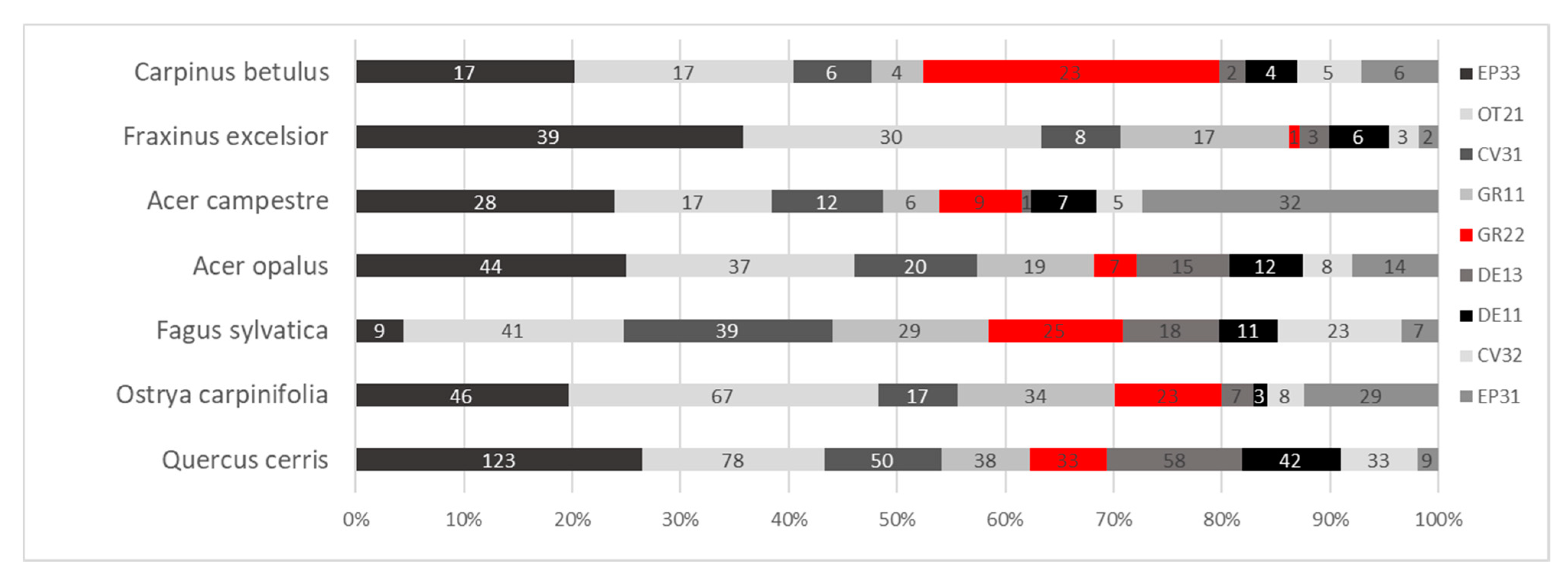
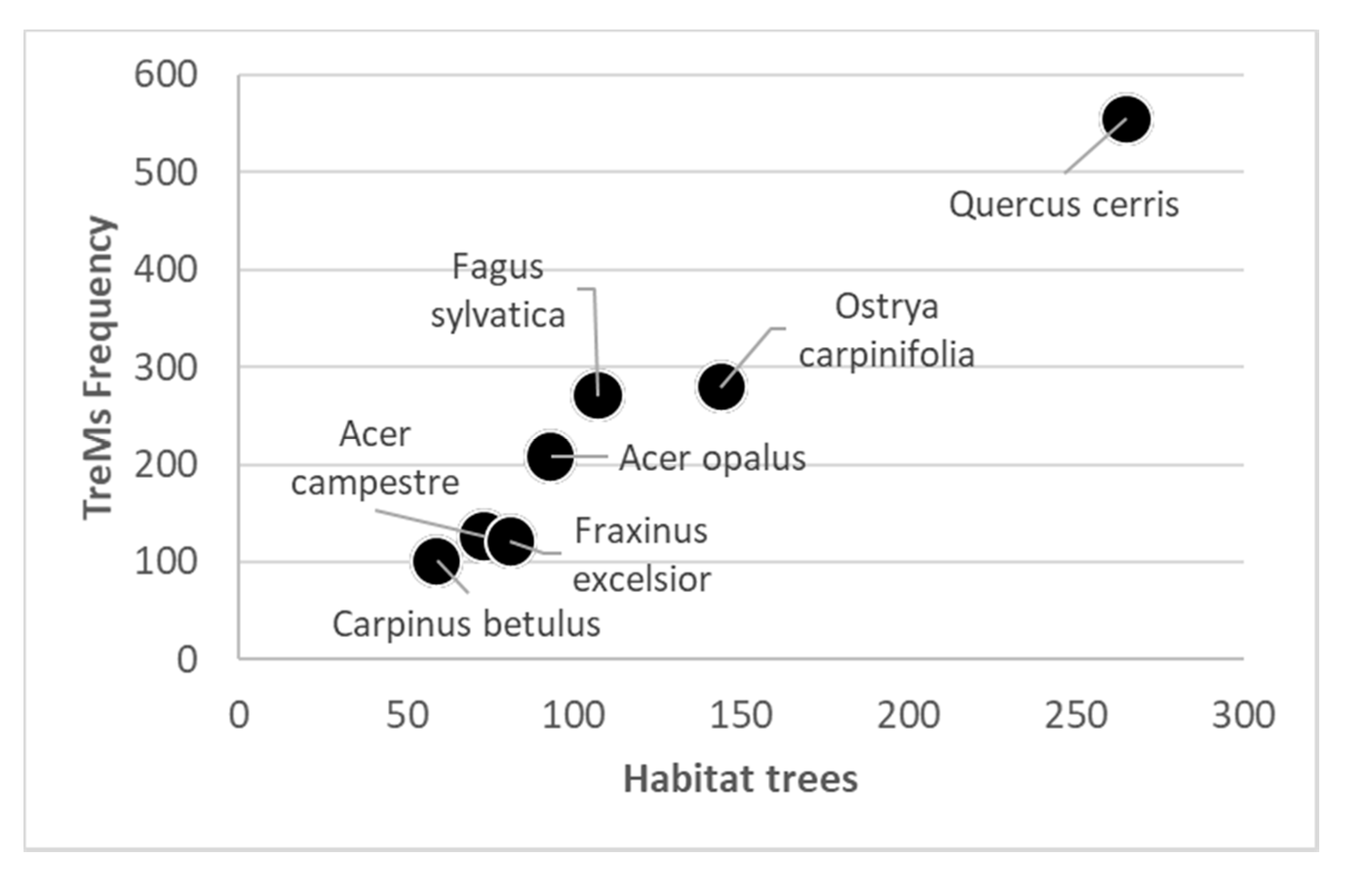
3.1. TreMs Occurrence and Abundance

A total of 40 out of 64 TreMs types were observed during the field survey, out of which seven represent 73% of the total amount (Table 2). The TreMs frequencies within the plots range between 14 and 101, while those for habitat trees fall between 8 and 51.
Lianas and crown microsoil are, in absolute terms, the most frequent TreMs encountered in the study area, representing 36% of the TreMs. The results highlight that cavities, such as rot-holes originating from branch breakage, and growth forms, such as root buttresses and water sprouts, are also rather frequent, representing 9% and 16%, respectively. Among deadwood, dead branches of small diameter are more frequent than dead branches with large diameters, and those that are not sun-exposed are more frequent than those that are sun-exposed.

3.2. Predicting TreMs and Habitat Trees Using ALS Metrics

The predictive abilities of the Random forest algorithm in the identification of TreMs slightly differs among the levels of the hierarchical classification, with NMAE values that range between 0.249 and 0.429 (Table 3). Overall, similar average values of the NMAE were observed for all the hierarchical levels. However, slightly better performance was reached for TreMs CAT-2 (0.270), while Single TreMs was the worst-predicted category (0.294), and the categories TreMs CAT-1 and TreMs SUM showed intermediate values equal to 0.287.
Looking at the level 1, though not clearly marked, the predictive performance increases with the frequency of TreMs, for which abundant TreMs such as DE13, GR22, and CV31 are more detectable than less frequent TreMs such as EP31, GR12, and DE11. More precisely, DE13 and GR22 are those microhabitats for which the best results were observed, 0.249 (SE = 0.067) and 0.259 (SE = 0.102), respectively. On the contrary, EP31 and GR12 showed NMAE values of 0.429 (SE = 0.268) and 0.355 (SE = 0.111), respectively (Table 3). The remaining TreMs presented NMAE values that ranged between 0.265 and 0.289.
As for TreMs CAT-1 prediction, the results show an NMAE value ranging from 0.251 to 0.364, for CV3 (SE = 0.072) and CV4 (SE = 0.174), respectively. In this case, less frequent microhabitats are poorly detectable.
Looking at level 3, the worst performance was obtained for GR (NMAE = 0.283; SE = 0.099) and DE (NMAE = 0.282; SE = 0.048), while CV is the microhabitat category for which the best performance was obtained, showing an NMAE of 0.252 (SE = 0.079). In this case, the variability of the NMAE is very low, and the performance can be considered satisfactory.
At level 4, the Random forest algorithm achieved similar predictive performance for both variables, showing NMAE values of 0.286 (SE = 0.073) for Count TreMs and 0.287 (SE = 0.079) for habitat trees.

3.3. Ranking Metrics Contribution in Predicting Microhabitat Abundance

In absolute terms, cov_gap, max, and c03 are the most recurrent ALS metrics, which contributed to predicting most of the microhabitat types and categories (Figure 3). However, the combination of ALS metrics in the prediction is not fixed, but the selection of metrics changes for the prediction of each microhabitat type and category.
For example, at level 1, the most recurrent metrics are cov_gap (for CV31, CV32, DE11, GR11, GR12, and GR22), c03 (for CV31, CV32, DE11, GR11, and OT21), d02 (for DE11, EP33, GR22, and OT21), and kur (for CV31, EP31, EP33, and GR12), while the less recurrent ones are c01, p01, and b90, which were selected only once for the prediction of OT21, GR22, and GR11, respectively.
Nevertheless, looking at EP31 (i.e., the best predicted TreMs), the model selected b70, d00, kur, and c04 as contributing ALS metrics in the prediction. Particularly, b70 (the percentage of ALS returns whose heights are below 70% of the maximum tree height, after the subtraction of the height cut-off value) is the most important predictor, contributing to about 60% of the prediction of EP31 (Figure 4). Moreover, a positive relationship between the predictor and EP31 was observed, even if the sigmoid curve indicates that there is a peak that marks the end of the positive trend for higher values of b70.
The most recurrent ALS metrics for TreMs CAT-1 prediction are cov_gap (CV3, EP3, GR1, and GR2) and c03 (CV3, CV4, and GR1), while d00 and b70 are never selected. The results show that four predictors (c03, d02, c04, and c01) allow the prediction of CV4. Moreover, a positive trend between CV4 and c03, which is the most important predictor, was observed, even if there is a slightly negative trend with higher values of c03.
The most recurrent ALS metrics for TreMs CAT-2 are max (CV, DE, EP, and GR), c03 (CV, GR, and OT), and cov_gap (CV, DE, and GR), while c04 is the only metric that is never selected.
The results show that GR prediction requires the c03, cov_gap, max, and p01 predictors, of which c03 is the most important predictor.
At level 4, the most recurrent ALS metrics are max and c04, which contributed to predicting both Count TreMs and habitat trees. Conversely, d02, c03, d00, kur, and c01 are those ALS metrics that are not selected by the model for the prediction of TreMs SUM categories. Particularly, max is the most important ALS metric, representing over 70% variable importance for the prediction of habitat trees, showing a negative relationship.

4. Discussion

In this study, we presented a new approach to predicting the abundance of microhabitats and habitat trees within forests using ALS data. Metrics derived from ALS data have been used to evaluate many forest variables, such as the tree height, canopy density, and canopy stratification [20]. Our approach consisted of relating predictors derived from ALS point clouds with forestry attributes such as the abundance of TreMs using an ML algorithm (i.e., Random forest). The results showed that the Random forest algorithm exhibits good performance in predicting microhabitats belonging to the hierarchical classification. Nevertheless, some challenges are still unsolved due to the high variability among microhabitats, the unknown role played by tree species composition, and—more generally—the role played by forest structure, which is even more marked in mixed and stratified forests. Overall, the results can be considered satisficing compared to the difficulties and the efforts necessary for collecting forest inventory data in multi-layered forests, within which field surveys are also very challenging. The small size of the sample represents the most hindering factor for the better calibration of the algorithm. However, the approach can be easily applied at a larger scale offering great support for monitoring forest biodiversity. ALS data allow the identification of TreMs and habitat trees, fostering the development of predictive maps, which are very useful for assessing forest biodiversity at a large scale. For this reason, the use of remote sensing, particularly ALS data, could represent a cost-effective and powerful tool for the development of suitable ecological indicators based on the abundance of microhabitats.

4.1. TreMs Prediction and Forest Structure

As was expected, TreMs are more frequent on dominant trees (see Appendix A), as previously stated by many authors [4,5,6]. Their abundance is affected by forest structure [11,14] and can be balanced through silvicultural interventions retaining or removing large trees in the forests.
Moreover, if, on one hand, forestry can regulate the abundance of TreMs, on the other hand, the lack of silvicultural interventions for a long period and the consequent aging of trees, as in this study area [32,44], fostered the abundance of such TreMs that reflect the naturalness of the forest (e.g., lianas, crown microsoil, branch holes, and dead branches).
Regarding the forest structure characteristics, beyond the tree diameter, which is recognized to be useful for assessing the TreMs abundance [4,5], this study highlights that the tree height and the density of tree crowns also affect the assessment of TreMs abundance, especially with ALS devices. The results highlight that cov_gap, max, and c03 are the most important ALS metrics for predicting TreMs abundance. Such metrics describe the inverse of the canopy cover (i.e., the canopy gaps or density), the maximum height of all returns above the height cut-off (i.e., 1.30 m), and the number of returns between 20 and 30 meters, respectively (see Appendix B). However, a well-defined relationship between ALS metrics and the abundance of TreMs is missing, probably because of the small sample size. However, the study reveals that few ALS metrics allow the prediction of some individual microhabitats such as dead branches or lianas.
An overall negative relationship between tree height and the abundance of both TreMs and habitat trees was observed, even if it became positive for very high trees. The justification is that we have to expect to find more microhabitats in trees with large branches and crown area rather than on higher trees with a small crown. Assessing the ratio between the DBH and crown area of trees could represent an important index for assessing the abundance of TreMs.
The heterogeneity of tree heights—i.e., the vertical distribution of trees and tree crowns, especially in the mixed forests—is not an optimal condition for using ALS data to assess TreMs abundance. Usually, ALS allows the production of significant canopy height models, but for our purposes, it is important to have a high-resolution point cloud not only in the top layer but also in the intermediate canopy layers. Low-density point clouds in multi-layered forests might represent a crucial constraint to the detection of trees [45] and other forest inventory variables.
We observed that the predictive accuracy increases for forest stands with low-density crowns, which means poor amounts of leaves in the top layers (i.e., trees with large branches), and as a consequence, a more dense point cloud is available in the intermediate layers, as shown by the relative variable importance of ALS metrics for predicting CV4 or also GR12, which often occur on trees with large diameters and large branches.
The results could be improved significantly by using highly dense point clouds, like those developed by Terrestrial Laser Scanners, especially for microhabitats such as bark structures, injuries, woods, cracks, scars, and fungi [29], but this entails higher costs for monitoring activities.

4.2. TreMs Hierarchical Prediction

Observing and counting TreMs in the field is very challenging and, often, the efforts are sustainable only for research issues rather than for practical management. The outcomes of this study demonstrate that ALS data might support the prediction of TreMs and habitat tree abundance, even if numerous efforts are necessary to improve the accuracy of prediction. Looking at the hierarchical levels, the predictive accuracy differs among levels as well as among the TreMs of the same level. Overall, better results were observed for TreMs CAT-2 (level 3) and for some TreMs at single level.
At single level, better predictive accuracy was obtained for TreMs that occur on large trees and which often occupy the top and the higher layers of canopy such as DE13 (dead branches ø 10–20 cm, ≥50 cm, not sun-exposed), CV31 (branch hole >5 cm), and OT21 (fork formed by branches with formation of microsoil). The predictive performance decreases for microhabitats, such as EP31 (epiphytic bryophytes, as mosses, covering more than 25% of the trunk), GR12 (root buttress cavities with entrance >10 cm large), and DE11 (dead branches and limbs ø 10–20 cm, sun-exposed), which are less frequent. The TreMs frequency affects the prediction performance, and the algorithm failed in the prediction of TreMs with frequencies lower than 50. For this reason, the prediction of TreMs such as “dendrotelms and water-filled holes” was possible only at level 2, where the single TreMs were grouped at the higher hierarchical level (CV4). Additionally, in this case, the high-density point clouds of intermediate-top layers—such as c03 (number of returns between 20 and 30 m)—impact the prediction accuracy. The prediction performance increased when moving from single level to the upper levels of the hierarchical classification, up to TreMs CAT-2. By contrast, the higher variability among the TreMs at level 4 slightly hinders the prediction of Count TreMs and habitat trees. Though this aspect could be partially tackled through a powerful LiDAR sensor, the variability among microhabitats remains very huge and could represent a bottleneck in the use of ALS for microhabitat prediction. However, in this study, the categories that resulted better detection at level 3 are somewhat linked to veteran trees, such as tree cavities. Furthermore, some characteristics that could be defined as “species-specific” are highlighted, e.g., GR for beech and for European hop-hornbeam, or EP for oak and maples. Nevertheless, further investigations are necessary to verify the correlation between TreMs occurrence and tree species [46].
Though the performance obtained at level 4, for both Habitats Trees and Count TreMs, was slightly worse, ALS data allow their detection. The huge variability of the TreMs types at this level, due to the cumulative effect, probably impacts the performance accuracy, even if the results can be considered satisficing. This is an important finding because it demonstrates that ALS data support forest management through the identification and mapping of TreMs abundance, fostering the identification of biodiversity hotspots.

4.3. TreMs as Biodiversity Indicators

The increased interest in the assessment of microhabitat abundance, at the European level, highlights how TreMs provide significant support to forest management with the final aim of integrating biodiversity conservation with the provision of other ecosystem services. With the recognition of the importance of TreMs and habitat trees for assessing forest biodiversity, the pan-European set of Criteria and Indicators for sustainable forest management can be significantly enriched and improved [47,48,49]. TreMs abundance can be considered a useful biodiversity indicator because they provide refuges for numerous living organisms [1], reflecting the habitat value of the trees and naturalness (e.g., the lack of silvicultural interventions over time) of forests [50].
The presence of TreMs—such as epiphytes, dendrotelms, and water-filled holes—indicates the long-term absence of silvicultural interventions, and they can be considered indicators of the aging of forest stands, such as for the deadwood [51,52]. The abundance of TreMs can be considered as a variable useful for the identification of forest functional destination units (e.g., [53]), such as biodiversity hotspots, and for defining forestry strategies to balance biodiversity conservation with the provision of other forest ecosystem services [5,54]. Assessing TreMs abundance can be beneficial not only in old-growth forests but also for supporting forest practitioners in the selection of standards in the coppice forests—which are very common in the Apennine mountains, representing about 40% of Italian forest area [55]—as well as for supporting forest management and planning [56,57].
Developing a more user-friendly method for predicting the occurrence and abundance of these ecological structures, based on forest inventory data, is strongly necessary for extending their assessment at the country level. In light of this, remote sensing will continue to, and increasingly, play a crucial role in the forest sector.

5. Conclusions

The detection of microhabitats in forests represents an emerging, but challenging, task for assessing forest biodiversity and for integrating biodiversity conservation in forest management with remote sensing techniques, which strongly supports the detection of these particular ecological niches, and it will continue to attract research interest.
In this study, we demonstrate that assessing the density and the stratification of ALS point clouds allows to predict the microhabitat abundance. Dense and stratified point clouds, especially in the intermediate and top layers, tally with the abundance of TreMs.
The frequency and diversity of microhabitat types impact the remote sensing predictive performance. Abundant microhabitats are easier to detect than less frequent microhabitats. The models used in this study highlight that abundance is predicted at all levels of hierarchical classification. However, the best performance was obtained at the Single TreMs level, for some microhabitats, and at the TreMs CAT-2 level.
Aspects of the forest structure, particularly the tree height and crown density, represent important predictors of TreMs and Habitat Tree abundance in terms of ALS data. The multi-layered nature of unevenly aged forest hinders the detection performance. TreMs that occur on the top layers of the canopy are more detectable than TreMs occurring on the bases of tree trunks, for which a dense point cloud is required.
Further investigations are necessary to distinguish between the role played by forest structure, and thus controlled through forestry, and the natural role played by tree species in the occurrence of TreMs.
In conclusion, ALS allows the prediction of the abundance of TreMs, but assessing their diversity remains challenging. Mapping TreMs abundance supports forest managers in planning activities, such as identifying forest patches or stands with high habitat value. Assessing the habitat value of forests could support the development of biodiversity indicators, such as forest naturalness, an indicator that could affect the social perception of the importance of forest functions and the ecosystem services that are provided.

Author Contributions

Conceptualization, G.S. and M.D.F.; methodology, M.D.F. and G.S.; software, M.D.F.; validation, M.B. and M.M. (Mauro Maesano); formal analysis, M.D.F.; investigation, G.S.; resources, B.L.; data curation, G.S.; writing—original draft preparation, G.S.; writing—review and editing, M.D.F., M.M. (Mauro Maesano):, M.B., and G.S.; supervision, M.M. (Marco Marchetti) All authors have read and agreed to the published version of the manuscript.

Acknowledgments

This research was supported by the LIFE program and the Italian Academy of Forest Sciences, in the framework of the project “FRESh LIFE—Demonstrating Remote Sensing integration in sustainable forest management” (LIFE14 ENV/IT/000414). We thank the Carabinieri Forestali of Montedimezzo for the logistic support provided during the field campaign.

Conflicts of Interest

No conflict of interest.

Appendix A

Forest Structure and TreMs Frequency According to Field Data

A total of 2380 trees were measured and observed within the 35 plots, with a DBH ranging from 2.5 cm to 104 cm and tree height ranging from 1.4 m to 39.6 m (Figure A1). Except for some outliers, Turkey oak and beech are the species that present larger trees, with higher variability, in terms of both tree DBH and tree height, with trees that are over 30 m in height (Q. cerris, F. sylvatica, F. excelsior, and C. betulus) representing most of the top canopy layer. It is interesting to note how trees of Abies alba are present only in the understory layer, probably due to the natural expansion of regeneration from mature pure and mixed stands, which are in the surrounding forest area [58].
Figure A1. Tree diameter and tree height distribution per tree species.
Remotesensing 12 02142 g0a1
The growing stock of the forests ranges between 183 and 647 m3 ha−1, with the numbers of trees per hectare varying from 454 to 3705. The forest is characterized by a total of 16 tree species, ranging from 3 to 11 species among plots.
Regarding the frequency of TreMs, in the study area were counted a total of 2484 TreMs, on 851 Habitat Trees.
Table A1. Descriptive statistics for the average values of DBH, maximum tree height, basal area and volume, tree and tree species abundance, habitat trees, and TreMs. The values are summarized per plot.
Volume (m3/ha)Basal Area (m2/ha)Tree Species (no.)Trees ha−1
(no.)
DBH (cm)Height Max (m)Habitat Trees (no.)TreMs (no.)
Min18319.94345411.3317.55814
1st Qu.302301.6769017.7424.921631
Median367367.47102021.2528.442044
Mean387387.47.5128521.2128.32449
3rd Qu.464463.79167323.730.883165
Max647647.211370531.9639.6351101
The abundance of TreMs is significant correlated with the dimensions of the trees [5]. TreMs frequency and variability increase with increments in both tree DBH and tree height.
Figure A2. TreMs frequency per species.
Remotesensing 12 02142 g0a2
Figure A3. Abundance of TreMs and Habitat Trees per species.
Remotesensing 12 02142 g0a3

Appendix B

Table A2. ALS metrics description. Metrics for which a variable importance was calculated are in bold and italics and indicated with *.
Metrics NameMetrics Description
max*Maximum height of all returns above the cutoff
minMinimum height of all returns above the cutoff
avgAverage height of all returns above the cutoff
StdStandard deviation of height of all returns above the cutoff
SkeReturns height skewness of points above the height cutoff
kur*Returns height kurtosis of points above the height cutoff
QavAverage square height of points above the height cutoff
dns.gapInverse of the canopy density. Canopy density is the number of points above the height cutoff divided by the number of all returns
d00*Relative height density as the total number of returns between 1.30 and 5 m divided by the total number of points and scaled to a percentage
d01Relative height density as the total number of returns between 5 and 10 m divided by the total number of points and scaled to a percentage
d02*Relative height density as the total number of returns between 10 and 20 m divided by the total number of points and scaled to a percentage
d03Relative height density as the total number of returns between 20 and 30 m divided by the total number of points and scaled to a percentage
d04Relative height density as the total number of returns > 30 m divided by the total number of points and scaled to a percentage
cov.gap*Inverse in the canopy cover. Canopy cover is the number of first returns above the height cutoff divided by the number of all first returns and output as a percentage
c00Number of returns between 1.30 and 5 m
c01*Number of returns between 5 and 10 m
c02Number of returns between 10 and 20 m
c03*Number of returns between 20 and 30 m
c04*Number of returns > 30 m
p01*Percentile 1 of height distribution
p05Percentile 5 of height distribution
p10Percentile 10 of height distribution
p25Percentile 25 of height distribution
p50Percentile 50 of height distribution
p75Percentile 75 of height distribution
p90Percentile 90 of height distribution
P95Percentile 95 of height distribution
p99Percentile 99 of height distribution
b10The percentage of ALS returns whose heights are below 10% of the maximum tree height, after the subtraction of the height cut-off value
b20The percentage of ALS returns whose heights are below 20% of the maximum tree height, after the subtraction of the height cut-off value
b30The percentage of ALS returns whose heights are below 30% of the maximum tree height, after the subtraction of the height cut-off value
b40The percentage of ALS returns whose heights are below 40% of the maximum tree height, after the subtraction of the height cut-off value
b50The percentage of ALS returns whose heights are below 50% of the maximum tree height, after the subtraction of the height cut-off value
b60The percentage of ALS returns whose heights are below 60% of the maximum tree height, after the subtraction of the height cut-off value
b70*The percentage of ALS returns whose heights are below 70% of the maximum tree height, after the subtraction of the height cut-off value
b80The percentage of ALS returns whose heights are below 80% of the maximum tree height, after the subtraction of the height cut-off value
b90*The percentage of ALS returns whose heights are below 90% of the maximum tree height, after the subtraction of the height cut-off value

References

  1. Bütler, R.; Lachat, T.; Larrieu, L.; Paillet, Y. Habitat trees: Key elements for forest biodiversity. In Integrative Approaches as an Opportunity for the Conservation of Forest Biodiversity; Kraus, D., Krumm, F., Eds.; European Forest Insititute: Joensuu, Finland, 2013; pp. 84–91. [Google Scholar]
  2. Großmann, J.; Schultze, J.; Bauhus, J.; Pyttel, P. Predictors of Microhabitat Frequency and Diversity in Mixed Mountain Forests in South-Western Germany. Forests 2018, 9, 104. [Google Scholar] [CrossRef] [Green Version]
  3. Leidinger, J.; Weisser, W.W.; Kienlein, S.; Blaschke, M.; Jung, K.; Kozak, J.; Fischer, A.; Mosandl, R.; Michler, B.; Ehrhardt, M.; et al. Formerly managed forest reserves complement integrative management for biodiversity conservation in temperate European forests. Biol. Conserv. 2020, 242, 108437. [Google Scholar] [CrossRef]
  4. Asbeck, T.; Pyttel, P.; Frey, J.; Bauhus, J. Predicting abundance and diversity of tree-related microhabitats in Central European montane forests from common forest attributes. For. Ecol. Manag. 2019, 432, 400–408. [Google Scholar] [CrossRef]
  5. Santopuoli, G.; di Cristofaro, M.; Kraus, D.; Schuck, A.; Lasserre, B.; Marchetti, M. Biodiversity conservation and wood production in a Natura 2000 Mediterranean forest. A trade-off evaluation focused on the occurrence of microhabitats. iForest-Biogeosciences For. 2019, 12, 76–84. [Google Scholar] [CrossRef]
  6. Paillet, Y.; Debaive, N.; Archaux, F.; Cateau, E.; Gilg, O.; Guilbert, E. Nothing else matters? Tree diameter and living status have more effects than biogeoclimatic context on microhabitat number and occurrence: An analysis in French forest reserves. PLoS ONE 2019, 14, e0216500. [Google Scholar] [CrossRef] [PubMed] [Green Version]
  7. Michel, A.K.; Winter, S. Tree microhabitat structures as indicators of biodiversity in Douglas-Fir forests of different stand ages and management histories in the Pacific Northwest, U.S.A. For. Ecol. Manag. 2009, 257, 1453–1464. [Google Scholar] [CrossRef]
  8. Kraus, D.; Schuck, A.; Bebi, P.; Blaschke, M.; Bütler, R.; Flade, M.; Heintz, W.; Krumm, F.; Lachat, T.; Larrieu, L.; et al. Spatially Explicit Database of Tree Related Microhabitats (TreMs). Version 1.2. Integrate+ Project; Institut National de la Recherche Agronomique (INRA): Paris, France, 2017. [Google Scholar]
  9. Larrieu, L.; Paillet, Y.; Winter, S.; Bütler, R.; Kraus, D.; Krumm, F.; Lachat, T.; Michel, A.K.; Regnery, B.; Vandekerkhove, K. Tree related microhabitats in temperate and Mediterranean European forests: A hierarchical typology for inventory standardization. Ecol. Indic. 2018, 84, 194–207. [Google Scholar] [CrossRef]
  10. Larrieu, L.; Cabanettes, A. Species, live status, and diameter are important tree features for diversity and abundance of tree microhabitats in subnatural montane beech-fir forests. Can. J. For. Res. 2012, 42, 1433–1445. [Google Scholar] [CrossRef]
  11. Vuidot, A.; Paillet, Y.; Archaux, F.; Gosselin, F. Influence of tree characteristics and forest management on tree microhabitats. Biol. Conserv. 2011, 144, 441–450. [Google Scholar] [CrossRef]
  12. Paillet, Y.; Bergès, L.; Hjältén, J.; Odor, P.; Avon, C.; Bernhardt-Römermann, M.; Bijlsma, R.-J.; De Bruyn, L.; Fuhr, M.; Grandin, U.; et al. Biodiversity differences between managed and unmanaged forests: Meta-analysis of species richness in Europe. Conserv. Biol. 2010, 24, 101–112. [Google Scholar] [CrossRef]
  13. Johann, F.; Schaich, H. Land ownership affects diversity and abundance of tree microhabitats in deciduous temperate forests. For. Ecol. Manag. 2016, 380, 70–81. [Google Scholar] [CrossRef]
  14. Regnery, B.; Paillet, Y.; Couvet, D.; Kerbiriou, C. Which factors influence the occurrence and density of tree microhabitats in Mediterranean oak forests? For. Ecol. Manag. 2013, 295, 118–125. [Google Scholar] [CrossRef]
  15. Cosyns, H.; Kraus, D.; Krumm, F.; Schulz, T.; Pyttel, P. Reconciling the Tradeoff between Economic and Ecological Objectives in Habitat-Tree Selection: A Comparison between Students, Foresters, and Forestry Trainers. For. Sci. 2019, 65, 223–234. [Google Scholar] [CrossRef]
  16. McRoberts, R.E.; Winter, S.; Chirici, G.; LaPoint, E. Assessing forest naturalness. For. Sci. 2012, 58, 294–309. [Google Scholar] [CrossRef]
  17. Antonucci, S.; Rossi, S.; Deslauriers, A.; Morin, H.; Lombardi, F.; Marchetti, M.; Tognetti, R. Large-scale estimation of xylem phenology in black spruce through remote sensing. Agric. For. Meteorol. 2017, 233, 92–100. [Google Scholar] [CrossRef]
  18. Congedo, L.; Sallustio, L.; Munafò, M.; Ottaviano, M.; Tonti, D.; Marchetti, M. Copernicus high-resolution layers for land cover classification in Italy. J. Maps 2016, 12, 1195–1205. [Google Scholar] [CrossRef] [Green Version]
  19. Montaghi, A.; Corona, P.; Dalponte, M.; Gianelle, D.; Chirici, G.; Olsson, H. Airborne laser scanning of forest resources: An overview of research in Italy as a commentary case study. Int. J. Appl. Earth Obs. Geoinf. 2013, 23, 288–300. [Google Scholar] [CrossRef] [Green Version]
  20. Mura, M.; McRoberts, R.E.; Chirici, G.; Marchetti, M. Estimating and mapping forest structural diversity using airborne laser scanning data. Remote Sens. Environ. 2015, 170, 133–142. [Google Scholar] [CrossRef]
  21. Santi, E.; Paloscia, S.; Pettinato, S.; Fontanelli, G.; Mura, M.; Zolli, C.; Maselli, F.; Chiesi, M.; Bottai, L.; Chirici, G. The potential of multifrequency SAR images for estimating forest biomass in Mediterranean areas. Remote Sens. Environ. 2017, 200, 63–73. [Google Scholar] [CrossRef]
  22. Chirici, G.; McRoberts, R.E.; Fattorini, L.; Mura, M.; Marchetti, M. Comparing echo-based and canopy height model-based metrics for enhancing estimation of forest aboveground biomass in a model-assisted framework. Remote Sens. Environ. 2016, 174, 1–9. [Google Scholar] [CrossRef]
  23. Giannetti, F.; Puletti, N.; Puliti, S.; Travaglini, D.; Chirici, G. Assessment of UAV photogrammetric DTM-independent variables for modelling and mapping forest structural indices in mixed temperate forests. Ecol. Indic. 2020, 117. [Google Scholar] [CrossRef]
  24. Giannetti, F.; Chirici, G.; Gobakken, T.; Næsset, E.; Travaglini, D.; Puliti, S. A new approach with DTM-independent metrics for forest growing stock prediction using UAV photogrammetric data. Remote Sens. Environ. 2018, 213, 195–205. [Google Scholar] [CrossRef]
  25. Marcelli, A.; Mattioli, W.; Puletti, N.; Chianucci, F.; Gianelle, D.; Grotti, M.; Chirici, G.; D’Amico, G.; Francini, S.; Travaglini, D.; et al. Large-Scale two-phase estimation of wood production by poplar plantations exploiting sentinel-2 data as auxiliary information. Silva Fenn. 2020, 54, 15. [Google Scholar] [CrossRef] [Green Version]
  26. Maselli, F.; Chiesi, M.; Mura, M.; Marchetti, M.; Corona, P.; Chirici, G. Combination of optical and LiDAR satellite imagery with forest inventory data to improve wall-to-wall assessment of growing stock in Italy. Int. J. Appl. Earth Obs. Geoinf. 2014, 26, 377–386. [Google Scholar] [CrossRef]
  27. Lasserre, B.; Chirici, G.; Chiavetta, U.; Garfì, V.; Tognetti, R.; Drigo, R.; DiMartino, P.; Marchetti, M. Assessment of potential bioenergy from coppice forests trough the integration of remote sensing and field surveys. Biomass Bioenergy 2011, 35, 716–724. [Google Scholar] [CrossRef]
  28. Giannetti, F.; Puletti, N.; Quatrini, V.; Travaglini, D.; Bottalico, F.; Corona, P.; Chirici, G. Integrating terrestrial and airborne laser scanning for the assessment of single-tree attributes in Mediterranean forest stands. Eur. J. Remote Sens. 2018, 51, 795–807. [Google Scholar] [CrossRef] [Green Version]
  29. Rehush, N.; Abegg, M.; Waser, L.T.; Brändli, U.-B. Identifying Tree-Related Microhabitats in TLS Point Clouds Using Machine Learning. Remote Sens. 2018, 10, 1735. [Google Scholar] [CrossRef] [Green Version]
  30. Zhou, T.; Popescu, S.C.; Lawing, A.M.; Eriksson, M.; Strimbu, B.M.; Bürkner, P.C. Bayesian and classical machine learning methods: A Comparison for tree species classification with LiDAR waveform signatures. Remote Sens. 2018, 10, 39. [Google Scholar] [CrossRef] [Green Version]
  31. Barabesi, L.; Franceschi, S.; Marcheselli, M. Properties of design-based estimation under stratified spatial sampling with application to canopy coverage estimation. Ann. Appl. Stat. 2012, 6, 210–228. [Google Scholar] [CrossRef] [Green Version]
  32. Frate, L.; Carranza, M.L.; Garfì, V.; Di Febbraro, M.; Tonti, D.; Marchetti, M.; Ottaviano, M.; Santopuoli, G.; Chirici, G. Spatially explicit estimation of forest age by integrating remotely sensed data and inverse yield modeling techniques. IForest 2016, 9, 63–71. [Google Scholar] [CrossRef] [Green Version]
  33. Kraus, D.; Bütler, R.; Krumm, F.; Lachat, T.; Larrieu, L.; Mergner, U.; Paillet, Y.; Rydkvist, T.; Schuck, A.; Winter, S. Catalogue of Tree Microhabitats—Reference Field List; Integrate+TechnicalPaper.16p; European Forest Institute: Freiburg, Germany, 2016. [Google Scholar]
  34. Hengl, T.; Walsh, M.G.; Sanderman, J.; Wheeler, I.; Harrison, S.P.; Prentice, I.C. Global mapping of potential natural vegetation: An assessment of machine learning algorithms for estimating land potential. PeerJ 2018, 6, e5457. [Google Scholar] [CrossRef] [PubMed] [Green Version]
  35. Liaw, A.; Wiener, M. Classification and Regression by randomForest. R News 2002, 2, 18–22. [Google Scholar]
  36. Breiman, L. Random forests. Mach. Learn. 2001, 45, 5–32. [Google Scholar] [CrossRef] [Green Version]
  37. Tompalski, P.; White, J.C.; Coops, N.C.; Wulder, M.A. Demonstrating the transferability of forest inventory attribute models derived using airborne laser scanning data. Remote Sens. Environ. 2019, 227, 110–124. [Google Scholar] [CrossRef]
  38. Kuhn, M. Building predictive models in R using the caret package. J. Stat. Softw. 2008, 28, 1–26. [Google Scholar] [CrossRef] [Green Version]
  39. Vabalas, A.; Gowen, E.; Poliakoff, E.; Casson, A.J. Machine learning algorithm validation with a limited sample size. PLoS ONE 2019, 14, 1–20. [Google Scholar] [CrossRef] [PubMed]
  40. Harrell, F.E., Jr.; Lee, K.L.; Mark, D.B. Multivariable prognostic models: Issues in developing models, evaluating assumptions and adequacy, and measuring and reducing errors. Stat. Med. 1996, 15, 361–387. [Google Scholar] [CrossRef]
  41. Breiner, F.T.; Guisan, A.; Bergamini, A.; Nobis, M.P. Overcoming limitations of modelling rare species by using ensembles of small models. Methods Ecol. Evol. 2015, 6, 1210–1218. [Google Scholar] [CrossRef]
  42. Di Febbraro, M.; D’Amen, M.; Raia, P.; De Rosa, D.; Loy, A.; Guisan, A. Using macroecological constraints on spatial biodiversity predictions under climate change: The modelling method matters. Ecol. Model. 2018, 390, 79–87. [Google Scholar] [CrossRef]
  43. Botchkarev, A. A new typology design of performance metrics to measure errors in machine learning regression algorithms. Interdiscip. J. Inf. Knowl. Manag. 2019, 14, 45–76. [Google Scholar] [CrossRef] [Green Version]
  44. Parisi, F.; Di Febbraro, M.; Lombardi, F.; Biscaccianti, A.B.; Campanaro, A.; Tognetti, R.; Marchetti, M. Relationships between stand structural attributes and saproxylic beetle abundance in a Mediterranean broadleaved mixed forest. For. Ecol. Manag. 2019, 432, 957–966. [Google Scholar] [CrossRef]
  45. Sačkov, I.; Santopuoli, G.; Bucha, T.; Lasserre, B.; Marchetti, M. Forest inventory attribute prediction using lightweight aerial scanner data in a selected type of multilayered deciduous forest. Forests 2016, 7, 307. [Google Scholar] [CrossRef] [Green Version]
  46. Király, I.; Nascimbene, J.; Tinya, F.; Ódor, P. Factors influencing epiphytic bryophyte and lichen species richness at different spatial scales in managed temperate forests. Biodivers. Conserv. 2013, 22, 209–223. [Google Scholar] [CrossRef] [Green Version]
  47. Maesano, M.; Lasserre, B.; Masiero, M.; Tonti, D.; Marchetti, M. First mapping of the main high conservation value forests (HCVFs) at national scale: The case of Italy. Plant Biosyst. 2016, 150, 208–216. [Google Scholar] [CrossRef]
  48. Santopuoli, G.; Ferranti, F.; Marchetti, M. Implementing Criteria and Indicators for Sustainable Forest Management in a Decentralized Setting: Italy as a Case Study. J. Environ. Policy Plan. 2016, 18, 177–196. [Google Scholar] [CrossRef]
  49. Wolfslehner, B.; Baycheva-Merger, T. Evaluating the implementation of the Pan-European Criteria and indicators for sustainable forest management—A SWOT analysis. Ecol. Indic. 2016, 60, 1192–1199. [Google Scholar] [CrossRef]
  50. Winter, S.; Möller, G.C. Microhabitats in lowland beech forests as monitoring tool for nature conservation. For. Ecol. Manag. 2008, 255, 1251–1261. [Google Scholar] [CrossRef]
  51. Lombardi, F.; Lasserre, B.; Chirici, G.; Tognetti, R.; Marchetti, M. Deadwood occurrence and forest structure as indicators of old-growth forest conditions in Mediterranean mountainous ecosystems. ECOSCIENCE 2012, 19, 344–355. [Google Scholar] [CrossRef]
  52. Pioli, S.; Antonucci, S.; Giovannelli, A.; Traversi, M.L.; Borruso, L.; Bani, A.; Brusetti, L.; Tognetti, R. Community fingerprinting reveals increasing wood-inhabiting fungal diversity in unmanaged Mediterranean forests. For. Ecol. Manag. 2018, 408, 202–210. [Google Scholar] [CrossRef]
  53. Vizzarri, M.; Chiavetta, U.; Santopuoli, G.; Tonti, D.; Marchetti, M. Mapping forest ecosystem functions for landscape planning in a mountain Natura2000 site, Central Italy. J. Environ. Plan. Manag. 2014, 0568, 1–25. [Google Scholar] [CrossRef]
  54. Pastorella, F.; Giacovelli, G.; Maesano, M.; Paletto, A.; Vivona, S.; Veltri, A.; Pellicone, G.; Mugnozza, G.S. Social perception of forest multifunctionality in southern Italy: The case of Calabria Region. J. For. Sci. 2016, 62, 366–379. [Google Scholar] [CrossRef] [Green Version]
  55. Gasparini, P.; Tabacchi, G. L’Inventario Nazionale delle Foreste e dei serbatoi forestali di Carbonio INFC 2005. Secondo inventario forestale nazionale italiano. In Metodi e Risultati; Edagricole-Il Sole 24 ore: Bologna, Italy, 2011; p. 653. [Google Scholar]
  56. Santopuoli, G.; Requardt, A.; Marchetti, M. Application of indicators network analysis to support local forest management plan development: A case study in Molise, Italy. iForest-Biogeosci. For. 2012, 5, 31–37. [Google Scholar] [CrossRef] [Green Version]
  57. Maesano, M.; Ottaviano, M.; Lidestav, G.; Lasserre, B.; Matteucci, G.; Mugnozza, G.S.; Marchetti, M. Forest certification map of Europe. IForest 2018, 11, 526–533. [Google Scholar] [CrossRef]
  58. Santopuoli, G.; Lasserre, B.; Di Martino, P.; Marchetti, M. Dynamics of the silver fir (Abies alba Mill.) natural regeneration in a mixed forest in the Central Apennine. Plant Biosyst. 2016, 150, 217–226. [Google Scholar] [CrossRef]
Figure 1. Study area. Geographical distribution of field plots within which forest inventory variables were collected. The sampling scheme was developed under the project FRESh LIFE using the one-per-stratum stratified sampling scheme [31].
Remotesensing 12 02142 g001
Figure 2. Airborne Laser Scanning (ALS) point cloud. Tile of ALS point cloud showing the heterogeneity of the forest stand structure. The density of points was higher for the uppermost trees and lower for the ground due to the dense canopy of tree crowns, which hinders the vertical penetration of the pulses.
Remotesensing 12 02142 g002
Figure 3. Spider plots depicting the ALS metrics’ recurrence. The dots indicate the number of times that the 11 ALS metrics were selected for microhabitat prediction among hierarchical classification levels.
Remotesensing 12 02142 g003
Figure 4. Variable importance (blue bars) and response curves (red lines) of the best-predicted microhabitats for each hierarchical classification. The gray curves indicate the response shapes of the 35 Random forest models derived from the five-times-repeated, seven-fold cross-validation, while the red curves show their average tendencies as calculated by a Loess estimator.
Remotesensing 12 02142 g004
Table 1. Tree-related Microhabitat (TreM) hierarchical classification (source: Kraus et al. 2016). Level 4, named TreMs SUM, is not reported here because it is not dependent on the type of TreMs but only on their occurrence on the trees, often including different TreMs types. Microhabitats that are not encountered in the forest are marked with *.
Single TreMs TreMs CAT-1TreMs CAT-2Single TreMs TreMs CAT-1TreMs CAT-2
CV11*Woodpecker cavitiesCavities (CV)BA11Bark pocketsBark (BA)
CV12BA12
CV13*BA21*Bark structure
CV14DE11Dead branches and limbs/crown deadwoodDeadwood (DE)
CV15*DE12
CV21Trunk and mold cavitiesDE13
CV22*DE14
CV23DE15*
CV24GR11Root buttress cavitiesDeformation/growth form (GR)
CV25GR12
CV26*GR13*
CV31Branch holeGR21Witches broom
CV32GR22
CV33GR31Cankers and burrs
CV41Dendrotelms and water-filled holesGR32
CV42EP11*Fruiting bodies fungiEpiphytes (EP)
CV43EP12*
CV44EP13*
CV51Insect galleries and bore holesEP14*
CV52*EP21Myxomycetes
IN11*Bark loss/exposed sapwoodInjuries and wounds (IN)EP31Epiphytic crypto- andphanerogams
IN12*EP32
IN13EP33
IN14*EP34*
IN21Exposed heartwood/trunk and crown breakageEP35*
IN22NE11*Vertebrate nestsNests (NE)
IN23NE12*
IN24*NE21Invertebrate nests
IN31Cracks and scarOT11*Sap and resin runOther (OT)
IN32OT12*
IN33OT21Microsoil
IN34*OT22
Table 2. TreMs frequency. The list refers to the TreMs frequencies within all 35 plots. The record “Other” refers to 23 TreMs types that present individual frequencies lower than 10.
TreMs CodeTreMs TypeFrequency of TreMsFrequency (%)
EP33Lianas, coverage > 25 %32418.89
OT21Crown microsoil29617.26
CV31Branch hole ø ≥ 5 cm1538.92
GR11Root buttress cavities ≥ 5 cm1518.80
GR22Water sprout 1217.06
DE13Dead branches and limbs ø 10–20 cm, not sun-exposed1076.24
EP31Epiphytic bryophyte coverage > 25 %1005.83
CV32Branch hole ø ≥ 10 cm885.13
DE11Dead branches and limbs ø 10–20 cm, sun-exposed885.13
GR12Root buttress cavities ≥ 10 cm663.85
CV44Dendrotelms and water-filled holes ø ≥ 15 cm/crown382.22
GR32Decayed canker, ø > 20 cm301.75
CV33Hollow branch, ø ≥ 10 cm281.63
CV12Woodpecker cavities ø = 5–6 cm241.40
DE14Dead branches and limbs ø > 20 cm, not sun-exposed160.93
CV43Dendrotelms and water-filled holes ø ≥ 5 cm/crown130.76
DE12Dead branches and limbs ø > 20 cm, sun exposed100.58
Others Other TreMs623.6
Table 3. Random forest predictive performance. For each microhabitat variable, the NMAE (Normalized Mean Absolute Error) and the standard error (SE) are reported.
TreMsNMAESE
Single TreMsCV310.2650.069
CV320.2870.103
DE110.2890.076
DE130.2490.067
EP310.4290.268
EP330.2700.067
GR110.2720.098
GR120.3550.111
GR220.2590.102
OT210.2670.097
TreMs CAT-1CV30.2510.072
CV40.3640.174
EP30.2780.061
GR10.2690.082
GR20.2750.086
TreMs CAT-2CV0.2520.079
DE0.2820.048
EP0.2630.051
GR0.2830.099
OT0.2690.076
TreMs SUMHabitat Trees0.2870.079
Count TreMs0.2860.073

