Semantic Segmentation for SAR Image Based on Texture Complexity Analysis and Key Superpixels


1
Key Laboratory of Intelligent Perception and Image Understanding of Ministry of Education, School of Artificial Intelligence, Xidian University, Xi’an 710071, China
2
Extreme Robotics Laboratory, University of Birmingham, Edgbaston B15 2TT, UK
*
Author to whom correspondence should be addressed.
Remote Sens. 2020, 12(13), 2141; https://doi.org/10.3390/rs12132141
Submission received: 4 June 2020
/
Revised: 25 June 2020
/
Accepted: 27 June 2020
/
Published: 3 July 2020
Abstract
:In recent years, regional algorithms have shown great potential in the field of synthetic aperture radar (SAR) image segmentation. However, SAR images have a variety of landforms and a landform with complex texture is difficult to be divided as a whole. Due to speckle noise, traditional over-segmentation algorithm may cause mixed superpixels with different labels. They are usually located adjacent to two areas or contain more noise. In this paper, a new semantic segmentation method of SAR images based on texture complexity analysis and key superpixels is proposed. Texture complexity analysis is performed and on this basis, mixed superpixels are selected as key superpixels. Specifically, the texture complexity of the input image is calculated by a new method. Then a new superpixels generation method called neighbourhood information simple linear iterative clustering (NISLIC) is used to over-segment the image. For images with high texture complexity, the complex areas are first separated and key superpixels are selected according to certain rules. For images with low texture complexity, key superpixels are directly extracted. Finally, the superpixels are pre-segmented by fuzzy clustering based on the extracted features and the key superpixels are processed at the pixel level to obtain the final result. The effectiveness of this method has been successfully verified on several kinds of images. Comparing with the state-of-the-art algorithms, the proposed algorithm can more effectively distinguish different landforms and suppress the influence of noise, so as to achieve semantic segmentation of SAR images.
1. Introduction
Synthetic aperture radar (SAR) is a widely used remote sensing imaging system, which can produce high-resolution images and work under all time and all-weather conditions [1]. SAR images have found wide applications in resources, environment, archeology, military and so on [2]. SAR image have a variety of landforms, such as rivers, crops and residential areas. When interpreting SAR images, it is usually necessary to understand these different landforms as independent regions. The interpretation of an image is to get a reasonable description of the image after a series of processing. An important issue in the SAR image applications is the correct segmentation and identification of objectives [3]. As a basic work of SAR image interpretation, SAR image segmentation is to divide a SAR image into several non-overlapping and coherent regions. The pixels in the same region have similarities, while the pixels between different regions have different features [4]. Dividing SAR images into these meaningful areas helps to understand the image from a high level and is convenient for further processing and analysis. However, due to the special imaging mechanism, the SAR image itself contains many speckle noises [5]. This multiplicative noise makes the processing of SAR images very challenging.
According to the complexity of texture, the application scenarios of SAR image segmentation algorithm can be divided into simple texture (farm crops, water, etc.) scenes and complex texture (residential areas, etc.) scenes. Among various methods for SAR image segmentation, pixel-level algorithms have achieved good results. Since the processing unit is a single pixel, these methods can preserve the detailed information in the image. It also makes the algorithm susceptible to noise. These algorithms are usually suitable for simple texture scenes. In contrast, regional algorithms tend to outperform the pixel-level ones. A superpixel is a small image area having a uniform appearance generated by dividing an original image. These algorithms can preserve the structural information and improve the computational efficiency by replacing thousands of pixels with hundreds of superpixels [6]. However, since the mixed superpixels may exist in the over-segmented image, the segmentation effect largely depends on the over-segmentation algorithm. Neither of these two algorithms can accurately achieve the semantic segmentation for SAR images. Texture analysis and deep learning methods are effective tools of SAR semantic segmentation [7,8,9]. Deep learning methods are usually supervised and have high requirements on the sample data volume. In addition, texture analysis methods usually need classifier and most of them are only suitable for specific scene. As in reference [7], an unsupervised algorithm to identify the flooded areas from SAR images based on texture information derived from the grey-level co-occurrence matrices (GLCM) texture analysis. This method is only useful when identifying flooded and dry areas.
The pixel-level segmentation algorithm assigns a label to each pixel in the image. The most common one is the clustering algorithms. These methods usually obtain cluster centres by multiple iterations and the similarity measure [10]. Fuzzy techniques are widely used in clustering and the most representative one is fuzzy C means algorithm (FCM) [11]. The main idea of FCM algorithm is to decrease the value of the objective function by updating a fuzzy membership matrix and cluster centres iteratively and deblurring the membership matrix to get the cluster results [12]. Xiang et al. [13] proposed a kernel clustering algorithm with fuzzy factor (ILK_FCM), which used the local information of the image to execute wavelet transform. They also designed a new weight blur factor and added the kernel metrics in the iterative process. Shang et al. [14] proposed the immune clone clustering algorithm based on non-information (CKS_FCM). This algorithm first uses a multi-objective optimisation method to determine the cluster centres and the non-local mean information are added in the clustering process to overcome the effect of speckle noises. To solve the problem that clustering all pixels reduces the efficiency of the algorithm, Pham et al. [15] proposed to process SAR images point-by-point, which extracted key points in the image and only these key points are processed during the clustering. Based on this, Shang et al. [16] put forward the fast key pixel fuzzy clustering (FKP_FCM) algorithm. They only perform fuzzy clustering on key pixels and the clustering results are used to determine the labels of non-key pixels. This method can get very accurate segmentation results in a relatively short time.
The superpixel-level methods usually over-segment the image and extract the features of each superpixels, such as intensity [17], texture [18], edge [19] and so on. Then these features are used to classify the superpixels, pixels in the same superpixel have the same label. Including mean shift [20], a lot of over-segmentation algorithms have been proposed such as normalized cuts (Ncuts) [21], graph-based [22], watershed method [23], Turbo superpixels method [24] and simple linear iterative clustering (SLIC) [25]. SLIC is prominent among these algorithms, since it can produce superpixels quickly without sacrificing much of the segmentation accuracy [26]. SLIC uses k-means clustering method to efficiently generate superpixels, which is proposed by Achanta et al. [25]. However, pure superpixels and mixed superpixels both exist in the SAR images. The pixels in the pure superpixels are from a single class and the mixed superpixels are composed of pixels with different labels, which can seriously affect the accuracy of segmentation [6]. Therefore, when using regional algorithms to segment SAR image, the mixed superpixels should be processed accordingly. To this end, Xiang et al. [27] proposed a novel superpixel generation algorithm that used the pixel intensity and position similarity to modify the similarity measure of SLIC algorithm, so the proposed algorithm is suitable for SAR images. In order to improve the boundary compliance of superpixels, Zou et al. [28] proposed that the SAR images can be modelled by a generalised gamma distribution to use the likelihood information of SAR image pixel clusters and the small isolated regions are removed in post-processing, which combined the spatial context and likelihood information. Qin et al. [29] improved cluster centre initialisation and introduced the SLIC method into polarimetric synthetic aperture radar (PolSAR) image processing, where the modified Wishart distance revised by the symmetric and was used for local iterative clustering. Wang et al. [30] integrated two different distances to measure the dissimilarity between adjacent pixels and introduced the entropy rate method into the oversegmentation of the PolSAR image. Jiao et al. [6] proposed a new concept, fuzzy superpixels, to reduce the generation of mixed superpixels. According to fuzzy superpixels, this method divided the pixels in the image into two parts: superpixels and pending pixels. The pending pixels are pixels in the overlapping search regions, which need further decision. That is, in fuzzy superpixels, not all pixels are assigned the same label.
The main problems to be solved in this paper is how to achieve land cover classification of SAR image and how to deal with the existence of mixed superpixels. Generally speaking, the more complex the application scenario and the greater the impact of noise, the more likely it is that mixed superpixels will appear. Therefore, in order to overcome the influence of mixed superpixels and speckle noise and improve the adaptability of the algorithm in different application scenarios, inspired by [16], we used superpixels to extend the key point idea to the regional level and proposed a method based on texture complexity analysis and key superpixel to achieve semantic segmentation. FCM can quickly converge and obtain accurate results, so we used the modified FCM to achieve the initial classification of superpixels. Since pixel-level method give each pixel a label and the pixels in mixed superpixels belong to different category, the pixel-level information is used to segment key superpixels. Specifically, the proposed algorithm calculates the texture complexity of the input image by a new texture analysis method, then neighbourhood information simple linear iterative clustering (NISLIC) is used to over-segment the image. For images with high texture complexity, the complex areas are first separated and key superpixels are selected according to certain rules. For images with low texture complexity, key superpixels are directly extracted. Finally, the superpixels are pre-segmented by fuzzy clustering based on the extracted features and the key superpixels are processed at the pixel level to obtain the final result. To make the result more smooth, we used a filtering method in the segmentation of key superpixels. The proposed algorithm not only uses texture analysis to improve the algorithm’s ability to segment complex texture scenes, but also overcomes the limitations of the over-segmentation algorithm on final result through the positioning and processing of key superpixels. In addition, the pixel-level information is used to determine the category of pixels in the key superpixels, which can retain more details and improve the accuracy of the segmentation.
The followings are the contributions of this paper:
- (1)
- To achieve land cover classification of a SAR image, a new texture complexity analysis method is proposed. The texture complexity of the input image is calculated using the change frequency of the grey value and the whole information can be grasped simply. The texture feature of each superpixels is also defined by this method which can separate superpixels located in complex landforms and superpixels located in simple landforms.
- (2)
- To overcome the impact of noise in over-segmentation, a new generation algorithm is proposed to improve the robustness of the superpixel generation to speckle noise, which uses the neighbourhood information of pixel to modify the similarity measure.
- (3)
- To deal with the existence of mixed superpixels, the concept of key superpixels is proposed. Key superpixels are mixed superpixels selected by certain rules. So, the segmentation no longer relies on the superpixel generation algorithm.
2. Methodology
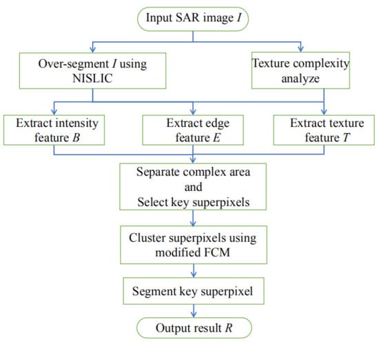
The pixel-level methods and the regional methods have achieved good performance on SAR images segmentation problem. Neither of these two algorithms can accurately achieve the semantic segmentation for SAR images. The pixel-level methods are slow and susceptible to noise. The regional methods are limited by the existence of mixed superpixels. In this paper, a new semantic segmentation method of SAR images based on texture complexity analysis and key superpixels is proposed (TKSFCM). Texture complexity analysis is performed and on this basis, mixed superpixels are selected as key superpixels. The framework of TKSFCM is shown in Figure 1.
2.1. Texture Complexity Analysis of SAR Images
Texture is important visual cues that describe the feature structure of a terrain surface in a finite sampling window. SAR images have a variety of landforms, such as rivers, crops and residential areas. Texture is an important tool for identifying land cover in SAR images and is widely used in SAR image segmentation [31,32,33]. So far, many methods have been proposed to extract texture features from SAR images, such as GLCM [34], and wavelet transform [35]. However, these methods are usually time-consuming because they require very complex calculations. On the basis of texture feature extraction, it is also necessary to segment the SAR image using a classifier or other methods.
Among different land covers, a residential area has the most disarray texture information. Since the grey value of this area is variable and contains obvious structures, the texture complexity of residential area is high. According to the complexity of the texture, different landforms in the SAR image can be divided into simple texture (farm crops, waters, etc.) and complex texture (residential areas, etc.). In image processing, information entropy is also often used to represent images. Since different texture regions are different in human visual perception, the spatial transformation frequency of grey values is different. The proposed algorithm is mainly for SAR images containing complex landforms. The texture information of the Ries image is analysed by showing its brightness change as shown in Figure 2.
Spatial variation of grey value in whole Ries image is shown in Figure 2a, where the x and y axis are the length and width of the Ries image, the z axis represents the grey values of the Ries image. It shows that the grey values of complex urban areas in the Ries image are large and varied. Figure 2b shows the grey histogram of complex residential area and farmland area, respectively. It can be seen intuitively that the grey histogram of complex residential areas fluctuates more than farm crops. Entropy of an image is a statistical form of a feature that reflects the agglomeration characteristics of the image distribution.
In this paper, a new SAR image texture recognition method is proposed to analyse the the texture complexity of the entire image. The texture complexity of each image can be divided as:
where p is the number of peaks in the greyscale histogram of the image. Due to the speckle noise, the max grey value of the input image is compressed to 100. For the different texture images represented by the red boxes in Figure 2, the compressed greyscale histogram is shown in Figure 3.
It can be seen from Figure 3 that the compressed greyscale histogram presents a relatively compact distribution. Figure 3a represents a complex residential area. Figure 3b represents a simple farmland area. The grey value of residential area changes frequently, multiple peaks and valleys appear with the change of grey value. Farmland area has a low change frequency of grey value, only a few sporadic peaks and valleys appear with the change of greyscale value. Therefore, using the number of peaks to calculate the texture complexity can directly distinguish the complex area and the simple area. Of course, speckle noise can cause the large grey change frequency. For images with greater noise impact, the texture complexity calculated by this method is higher. However, such images often produce mixed superpixels during the over-segmentation process, and these mixed superpixels contain more noise. Therefore, the texture complexity calculated by this method can be used as a reference for subsequent processing steps.
2.2. NISLIC
Assume that a SAR image containing N pixels is pre-segmented into K superpixels. In the standard SLIC algorithm, when performing local k-means clustering, the similarity between pixels is measured by the intensity and position of pixels. However, for SAR images, using only a single pixel value as the intensity constraint in the design process, the influence of the speckle noise is not considered. Therefore, we propose an improved version of SLIC named NISLIC, which uses the neighbourhood information of the pixel. When the pixel intensity in the single-channel SAR image follows the exponential distribution, refer to [30,36], the improved intensity distance between the pixel and the centre can be defined as:
where and represent two image blocks with same size centred on pixels i and j, respectively. , and represent the average intensity of these block and their union, respectively. The log-ratio operator is used to suppress the effects of speckle noise. M is the number of pixels in the image block. The use of image blocks instead of a single pixel is to capture local information around the pixel and reduce the effects of noise. Therefore, the size of the image block should not be too large, e.g., . The similarity measure of NISLIC is defined as:
where = is the spatial distances between the pixel and the centre. s = is the maximum spatial distance within the class. is a regularisation parameter that weights the relative contribution of and to the integrated distance . A larger indicates that is more significant than . Usually, the value of is chosen in [2,6]. Figure 4 intuitively shows the similarity measurement.
As shown in Figure 4, the light grey pixel block represents the search space of pixel i, and the dark grey pixel block is . Remaining blocks are the neighbourhood information of the cluster centres in the search space. The red line represents the spatial distance between pixel i and cluster centre j. The followings are the steps of NISLIC:
(1) Initialise the cluster centre, set K initial cluster centres on a regular grid spaced step apart and move the cluster centres to the lowest gradient position in the neighbourhood. (2) Allocate pixels, with the guidance of Equation (3), using local k-means clustering to assign each pixel to the nearest cluster centre in the search space. (3) Update the cluster centres and set each cluster centre as a corresponding pixel of the average value of all pixels. (4) Repeat steps (2)–(3) until the iteration condition is met. (5) Post-processing, use the connected component algorithm to merge small isolated regions into the nearest large superpixel.
A superpixel consists of a set of pixels that satisfy certain constraints, such as position, brightness, edges and texture. For example, if brightness is selected as a constraint, pixels in the same superpixels have almost the same brightness [17]. However, the standard SLIC algorithm does not consider noise effects. Therefore, although the SLIC algorithm can obtain superpixels with moderate size and sharp edges on the natural image, it is difficult to obtain accurate results in SAR images due to the speckle noise [13]. NISLIC uses pixel blocks instead of single pixel, which makes good use of neighbourhood information and overcomes this shortcoming to some extent. When only using the superpixel algorithm to segment SAR images, the labels of all the pixels in the same superpixel are the same. However, due to the mixed superpixels, the error rate of the segmentation result will be high. Therefore, in order to avoid the above situation, we select these mixed superpixels according to certain rules and segment them based on pre-segmentation to obtain more accurate results.
2.3. Feature Extraction of Superpixels
SAR images have their unique properties due to their different imaging mechanisms and captured scenes. For example, speckle noise exists in SAR images, and the presentation of the same topographical target is usually non-stationary [37] and has complex variations. Therefore, in order to segment SAR images accurately, it is necessary to extract effective features of superpixels to describe SAR images as comprehensively as possible. The pixel-level features, such as intensity, texture and edge, are commonly used to describe SAR images. In [17], the average level strategy is used to extend the pixel-level features to the superpixel-level: (1) for intensity and texture features, the feature of each superpixel is defined as the average of the corresponding features of all pixels in the superpixel; (2) for edge features, the features of any pair of adjacent superpixels are defined as the average of the edge features of all pixels along the boundary between them.
Firstly, the input image is linearly normalised to [0,1] to obtain the pixel-level intensity characteristics of the image. Then, the intensity average of all the pixels in the superpixel is taken as the intensity feature of the superpixel:
where b is the number of pixels in a superpixel. The second feature is texture. Using the grey-scale change frequency of the image, a new texture analysis method is proposed in this paper. Then the texture feature of a single superpixel is:
where p is the set of peak and valley values in greyscale histograms of the ith superpixel. is the occurrences number of the jth member in set p, is the intensity feature of the ith superpixel. This method can describe the texture features of each superpixel simply and intuitively. The complexity of complex landforms and simple landforms differ greatly. Therefore, the threshold method can be used to separate superpixels located in complex landforms and superpixels located in simple landforms.
The intensity features and texture features describe SAR image from different aspects. They are two important and complementary features of SAR image interpretation. Comparing to these features, the edge information of image can accurately position the boundaries between objects and is particularly helpful in characterizing gradually changing regions. Therefore, researchers proposed many methods for the edge extraction of SAR images [38,39,40,41]. Due to the coexistence of speckle noise and multi-scale objects, it is difficult to extract edges in a SAR image accurately. Reference [17], a multi-scale edge detector is used in this paper to extract edge features. The difference is that the number of edge points in each superpixel is taken as the edge feature of the superpixel:
where is the number of edge points in the ith superpixel in the jth edge image, and the edge points is extracted by Prewitt kernels.
2.4. Position Key Superpixels
When a SAR image is segmented by the over-segment method, the superpixels located inside the objects and obvious to be merged are called pure superpixels. The superpixels located between different objects and doubtful to merge are called superpixels with ambiguity [6], which is also called is the mixed superpixels. TKSFCM tries to extract and process these mixed superpixels as accurately as possible. Here, the mixed superpixels are called key superpixels. Key superpixels should have the following characteristics: (1) located between different objects, and (2) the features are significantly different from their neighbouring superpixels. Characteristic 1 indicates superpixels with a large edge feature value. Characteristic 2 represents that superpixels are more prominent in the neighbourhood. In order to facilitate uniform processing and comparison, the extracted superpixel features are first globally normalized:
where represents the original features of the ith superpixel (intensity , texture , edge ), and represent the maximum and the minimum of the features. To visualise the position of key superpixels during experiment, the value of each feature is normalised to [0,255] through Equation (7). Then, calculate the neighbourhood average deviation (NAD) of the intensity feature and the texture feature of the ith superpixel:
where represents the normalised features of the ith superpixel (intensity , texture ).
where N is the set of the adjacent superpixels of the ith superpixel. By calculating the NAD, the feature similarity relationship between a superpixel and its adjacent superpixels can be reflected. A larger NAD indicates that the adjacent superpixel is more prominent in the neighbourhood, meeting the characteristics 2. Taking intensity feature as an example, the calculation of NAD is shown in Figure 5.
As shown in Figure 5, the left is the intensity feature before calculating the NAD, and the right is the intensity feature after calculating the NAD. Referring to the label colour of Figure 4, taking the superpixel of label 5 as an example, its intensity characteristic value is 194 and the adjacent superpixels have label 2, 3, 4, 6 and 8. Calculating the NAD means to calculate the average of the difference between the adjacent superpixel and the superpixel of label 5. From the calculation results, the neighbourhood deviation values of the superpixels with the class labels of 4 and 5 are larger, which conform to the selection rules of key superpixels.
The edge feature extracted in this paper is the number of edge points contained in the superpixel. The more edge points in the superpixel, the more likely this super image exists between different objects, meeting the characteristics 1. Thus, a superpixel is called a key superpixel, when it satisfies the following condition:
where is the mean value of the edge feature. and represent the NAD of the intensity and the texture feature, respectively. The superpixel satisfying characteristics 1 or characteristics 2 is a key superpixel. However, for SAR images containing multiple landforms or complex areas, this method often divides all complex areas into key superpixels. This is because that the texture features of superpixels located in complex areas are greatly different from other superpixels. Therefore, the otsu algorithm is used to separate the complex and simple regions based on the extracted texture features. Then extract the key superpixels. Taking the Ries image (Figure 6a) as an example, Figure 6b is the separated complex area, and Figure 6c is the selected key superpixel.
It can be seen from Figure 6 that the area covered by the key superpixels substantially satisfies the characteristics of the mixed superpixels. Therefore, further subdivision of key superpixels can improve segmentation efficiency. The separated complex area basically covers the residential area in the Ries image. To facilitate further segmentation, superpixels in complex areas are given the same intensity characteristics, which is the maximum intensity feature of these superpixels.
2.5. The Segmentation of Superpixels
2.5.1. Fuzzy Clustering on All Superpixels
After over-segmenting a SAR image into superpixels, the next task is to cluster similar superpixels to obtain pre-segmentation results. In [42], FCM is used to cluster superpixels. Inspired by the fuzzy local information C-Means (FLICM) method, during fuzzy clustering, the texture features and spatial information of superpixels are added into the objective function as fuzzy factors in this paper:
where N is the number of superpixels, c is the number of clusters, m is the fuzzy factor. According to [41], the value of m is 2, is the intensity feature of the ith super pixel, is the intensity feature of the kth cluster centre, represents the fuzzy membership of the ith superpixel to the kth cluster centre, is a fuzzy factor and has the following form:
Since the intensity feature is not sufficient to describe a superpixel, we use to represent the weight of the adjacent superpixel on the ith superpixel, which consists of two parts, one is the spatial distance weight and the other is the texture distance weight:
where is the spatial distance weight, and is the texture distance weighs. is defined as follows:
is defined as follows:
where is the Euclidean distance of the ith superpixel and the centre of the adjacent superpixel . and represents the texture features of the ith superpixel and , respectively. For the ith superpixel, the neighbouring superpixels with the closest space distance and similar texture feature have a larger weight. Both the texture information and the spatial information are utilised, which can avoid the impact of clustering using only feature information. The clustering is executed through iteratively updating the fuzzy membership matrix U:
And the cluster center V:
Execute Equations (16) and (17) iteratively for many times until the number of iterations is equal to the maximum iteration number. Or when the maximum change of fuzzy membership in two consecutive iterations is smaller than a small threshold, then the iteration will be stopped. The labels of superpixels can be determined according to the final fuzzy membership matrix U.
2.5.2. Segment Key Superpixels
After positioning the key superpixels, we can determine the labels of the pixels in the key superpixel based on the pre-segmentation results. Clustering superpixels according to Equation (11) can make good use of the intensity and texture features of superpixels and the results obtained are more accurate. However, key superpixels with blurring need further segmentation. As a result that these pixels are often located between two different targets and the class labels are not the same, this paper uses the pre-segmented clustering results and uses the pixel-level feature information to determine the class label of the pixels in the key superpixels.
We use pixel-level feature information to determine the labels of pixels in key superpixels. The specific method is to compare the feature information of the pixel in the key superpixel with the feature of the centre point of the most similar non-key superpixel to obtain the most similar centre point and inherit the class label:
where represents the label of the kth pixel in the ith key superpixel. represents the label of the most similar non-key superpixel. The determination of the most similar non-key superpixel is as follows:
where is the set of the adjacent non-key superpixels of the ith key superpixel. is the euclidean distance between the kth pixel and the jth non-key superpixel, and represents the local mean of the kth pixel and the centre of the jth non-key superpixel. Since the segmentation of key superpixels is obtained using a pixel-level approach, the results are somewhat discrete. To avoid this, we use a neighbourhood filtering method to filter the pixels in the key superpixels. For each pixel in the key superpixels, calculate the label variance of the pixels in the domain. If the variance of the pixel is 0, the label of the pixel is corrected to the same label as the neighbourhood pixel.
3. Experimental Setups and Algorithm Evaluation
3.1. Experimental Setups
Both the simulated SAR images and the real SAR images are used to test the effectiveness of the proposed algorithm for SAR image segmentation. The simulated SAR images are obtained by artificially polluting the original noise-free images with speckle noises, as shown in Figure 7. The speckle noise is simulated by gamma distribution. As we can see from Figure 7, we obtain 1, 2, 4 and 6-look simulated SAR images, where the smaller the look of an image, the greater noises the image suffers. In this paper, two different noise-free images are used to generate synthetic SAR images, named SI1, SI2, as shown in Figure 7a,f.
There are four classes in SI1 image, and the grey values are 0, 85, 170 and 255, respectively. There are three classes in SI2 image, including a complex texture region and two simple texture regions. The simple texture region simulates the farmland and river of real SAR image. Compared with the noise image of SI1, the noise image of SI2 is more difficult to segment, because the SI2 image contains complex texture regions and the grey level of this region is close to the left texture area.
In addition to the synthetic SAR image, we also use four real SAR images to test the effectiveness of the algorithm, which are Maricopa image, Chinalake image, Terracut image and Ries image, as shown in Figure 8.
According to Figure 8, we can see that these four real SAR images have different types of land covers. These test images can show the effectiveness of segmentation algorithms in a detailed way. The Key Laboratory of Intelligent Perception and Image Understanding of Ministry of Education have purchased the copyright of these images. Table 1 shows the detailed information of these images.
The first real SAR image is called Maricopa with a size of . It was taken in the American Maricopa Agricultural Center near Arizona. This image was captured by an airborne SAR in Ku-band. According to Table 1, Maricopa can be divided into four regions, including three different kinds of crops and water. When segmenting this image, the cluster number is set to 4. The second real SAR image is Chinalake with a size of . Chinalake is a Ku-band SAR image from Sandia National Laboratories. The radar is carried by the Sandia Twin Otter aircraft. Data are processed into images in real time. The third image is named Terracut with a size of . According to Table 1, this image can be divided into four regions, including three different kinds of crops and buildings. The fourth real SAR image is called Ries with a size of . These two images are a part of the TerraSAR-X image which is named Terra in this paper. Terra was taken at 1 July 2007, 23:00 UTC. According to Table 1, the polarisation of Terra is HH and the acquisition mode is a high resolution spotlight mode.
Five state-of-the-art algorithms are chosen to be comparison algorithms to further verify the effectiveness of the proposed algorithm on SAR images segmentation. They are CKS_FCM [13], FKP_FCM [16], a SAR image segmentation algorithm based on thumbnails and similar neighbours THFCM [43], a fast fuzzy clustering algorithm based on superpixels SFFCM [44] and a fast SAR image segmentation method based on two-step superpixels generation and weighted CRF algorithm FWCRF [45]. CKS_FCM first determines the initial clustering centres by immune clone algorithm, and in order to overcome the effect of speckle noises this method adds the non-local information to the clustering process. FKP_FCM first divides the image into key points and non-key points, then clustering the key pixels only and labels the remaining pixels by the clustering results. THFCM first divides the image into pixel groups of similar size, and uses most of the similar pixel points in these pixel groups to form thumbnails that are double the size of the original image, then uses the fuzzy C-means algorithm to combine the neighbourhood information in the thumbnails. This thumbnail is subjected to pixel-level clustering and segmentation, and the pixel points in the original SAR image are hierarchically segmented according to the thumbnail segmentation results. SFFCM uses a multi-scale morphological gradient reconstruction (MMGR) operation to generate superpixels with good adaptive irregularities, and then uses the grey histogram of the superpixels to cluster them fuzzy to obtain the final segmentation result. FWCRF uses fast and robust fuzzy C-means clustering (FRFCM) to divide SAR images into homogeneous and heterogeneous regions. At the same time, SLICalgorithm is used to segment the image into superpixels. Finally, by using the density-based spatial clustering (DBSCAN) method of the noise-based application, superpixels belonging to the same class are merged.
3.2. Algorithm Evaluation
(1) Evaluation index
There are many metrics to assess the segmentation accuracy (SA), such as F1-score, Jaccard Index, Dice coefficient. Jaccard coefficient is defined as the ratio of the size of the intersection of two sets to the size of the union of two sets. SA is defined as the ratio of the total number of correctly classified pixels on the total number of pixels in the image. Jaccard coefficient and SA both calculates the overlap between the two sets. Dice coefficient is a similarity measure related to the Jaccard index. In this paper, we use SA to evaluate the quality of each segmentation result, which is widely used in the field of image segmentation [46]. SA is calculated as follows:
where c represents the number of clusters, is the set of pixels whose labels are i by the algorithm and is the set of pixels whose labels are i in the ground truth image. The ground truth of test images is labeled by ourselves referring the different landform in Google map. The range of SA is [0,1], and the bigger the SA indicates the better the segmentation result [47]. The distinguishing feature of VKSFCM is the key superpixels can accurately locate the edge information of the input image. We use another metric F1-Score to measure the segmentation of the edge regions, the F1 coefficient of each type is:
where k represents the kth category, is the accuracy of each category and is the recall rate of each category.
(2) The texture analysis ability
In this paper, the greyscale transformation frequency is used to analyse the texture complexity of the input image. In order to test the texture analysis ability of the algorithm, the texture complexity analysis is performed on the following SAR images with different texture characteristics. The results are shown in Figure 9.
It can be seen from Figure 9 that the method proposed in this paper can clearly distinguish images containing multiple landforms and single landform, which brings great convenience for subsequent processing. There are only farmlands with different grey levels in Figure 9a. There are both residential region and areas with flat textures in Figure 9b. For images with multiple landforms, TKSFCM separates the different landforms according to the texture complexity.
(3) The evaluation of NISLIC
The performance of the new over-segment method can be seen in Figure 10 which shows the superpixel generated by the standard SLIC and NISLIC.
The superpixel generated by NISLIC is robust to speckle noise shown in Figure 10. The tested SAR image in Figure 10 is less affected by noise and has more obvious edge features. This image is called Chinalake. Using this image can fully demonstrate the superiority of NISLIC. For the result of NISLIC (Figure 10b), the shape of the superpixels in the uniform area is basically rectangular without being affected by the image itself. As can be seen from the upper left area of these two images, for the edge area, NISLIC achieved a relatively good fit. For regions with complex structures in the image, although the shape of the neighbouring superpixels is irregular, it can well grasp the detailed features of the region.
An important parameter of NISLIC is which measures the spatial distance and the intensity distance. Here Maricopa image is used to test the boundary recall of NISLIC when takes different values. It is worth noting that the boundary recall of SLIC in Maricopa image is 0.8697. The number of superpixels is set as 400. The result is shown in Figure 11.
As shown in Figure 11, when > 1, the boundary recall numbers of NISLIC are larger than SLIC. As continues to increase, the number of boundary recalls gradually increases. The maximum was reached when = 6, then the numbers slowly declined.
4. Results
Five comparison algorithms and the proposed algorithm are used on all synthetic SAR images and real images. This section proves the superiority of the proposed algorithm in SAR image segmentation by analysing and comparing the segmentation results of each algorithm on each image.
4.1. Results of Simulated SAR Images
4.1.1. Results of Simulated SAR Images Generated from SI1
The results of the 1-look noisy image of SI1 segmented by six algorithms are shown in Figure 12. The reason why we only list the result images of 1-look noisy image is that this image suffers most speckle noises. By analysing each segmentation result of 1-look noisy image, we can more accurately compare the advantages and disadvantages of each method.
Figure 12 presents that TKSFCM, FKP_FCM and THFCM all get better segmentation results on 1-look noisy image of SI1, while the results of the other two algorithms are poor. Compared with other algorithms, as shown in Figure 12a, the segmentation result of TKSFCM is less affected by noise and has a high degree of edge coincidence. The segmentation results of THFCM also have a high degree of edge coincidence, but there is a misclassification in the place adjacent to the edge, as shown in Figure 12c. As a result that the pixel block used by this algorithm in constructing the thumbnail image is not consistent with the edge information in the image, which leads to the loss of some details. The segmentation result of FKP_FCM is also good, as shown in Figure 12b. However, the segmentation result still contains some pixels that are wrongly segmented, and the edges are not kept smoothly and accurately. This is because the results of non-key points are affected by speckle noise. In segmented image of FWCRF (Figure 12f), many pixels belonged to the green class were wrongly segmented. It is due to the fact that the SLIC used in this algorithm is difficult to obtain more accurate over-segmentation results on the image with high noise content, which leads to the fact that the final result is greatly affected by noise. The segmentation image obtained by CKS_FCM (Figure 12d) shows that the algorithm is also seriously affected by speckle noise, so that many pixels are wrongly segmented. The segmentation results of SFFCM (Figure 12e) showed irregular edges. Although huge green areas are wrongly divided into yellow areas, they performed better for other areas. It is because only the super-pixel grey histogram information cannot be used to accurately segment the speckle noise-rich SAR image.
In order to make more accurate and intuitive analysis of each algorithm, we use five kinds of compared algorithms and TKSFCM to get the simulated images based on SI1 test, as shown in Figure 7b–e. The class number is 4, the SA of each methods on each image as shown in Table 2. The best results and our results are shown in bold in this table.
According to Table 2, we can see that for all noise images of SI1, TKSFCM achieves the highest segmentation accuracy. With the decrease of noise influence, the segmentation accuracy of the four methods except FWCRF tends to increase. It shows that FWCRF produces relatively poor results for all noise images and is most affected by noise. When the level of noise changes from 2 to 4, the segmentation accuracy of FWCRF is slightly reduced. This is because that the original regions with similar greyscale of SI1 images affected by noise are mistakenly merged when merging super pixels. However, for SAR images with the lowest degree of noise pollution, better segmentation results can be obtained. It is due to the FWCRF method uses SLIC to segment and merge the images during image segmentation. For SAR images with less speckle noise content, this method produces better super-pixel effect. Similarly, CKS_FCM has a high precision for the segmentation results of noisy images with high visibility, but the SAs of this method is low when the images are seriously polluted by noise. The SAs processed by THFCM is high and the noise impact is less than that of FWCRF, and CKS_FCM. FKP_FCM has excellent segmentation results for SI1 images, it happens all due to the impact of speckle noise on the results can be reduced by using key point clustering and non-local information. For images with less noise impact, SFFCM performs well, which indicates that the algorithm is suitable for images with less noise.
4.1.2. Results of Simulated SAR Images Generated from SI2
For all noisy images of SI2 image, six methods are also used to segment them and the cluster number is set to be 3. As a result that the two regions have close grey values and the segmentation result of 1-look image is poorly visible, the segmentation results of 6-look image are shown in Figure 13. In Figure 13, yellow represents complex areas.
The segmentation result in Figure 13 shows that for the complex texture regions in the image, except for TKSFCM and SFFCM, the other four algorithms cannot accurately segment them. As a result that the grey value of the complex texture area is close to the left area and SFFCM only uses the grey information, these two categories are divided into one. Figure 13a shows that the segmentation result of TKSFCM are closest to the real image, and only a few pixels are incorrectly segmented. For simple texture areas, it can be seen from Figure 13b,c,f that the segmentation results of FKP_FCM, FWCRF and THFCM are less influenced by noise. This indicates that for images suffered less noise, the segmentation effect of these algorithms is good. From the result of CKS_FCM (Figure 13b), the segmentation result of this algorithm is greatly affected by speckle noise.
In order to further compare the segmentation results of each algorithm on the SI2 images, the SA of each method on the four noise images is shown in Table 3. The best results and our results are shown in bold in this table.
Table 3 shows that TKSFCM shows high superiority compared to other algorithms in the four noise images. This is because for images containing complex texture regions, the coherence of the results obtained by using superpixels as the processing unit is good. For the 1-look image, the SA is not ideal. This is because the texture analysis method used in this paper is based on the greyscale histogram and the greyscale change on the areas with heavy noise pollution is also very large. Compared to SI1 images, the SAs of CKS_FCM are less affected by noise because the segmentation effect of the algorithm does not change much in complex regions. At the same time, the segmentation accuracy of the SFFCM is also less affected by noise. This is because the superpixel greyscale histogram information is used to divide the texture area and the complex area into a category. In this case, the algorithm has a high edge fit and good regional coherence. Affected by noise, the SAs of FWCRF and TKSFCM fluctuates. In addition, as shown in Table 3, FKP_FCM and THFCM achieve high segmentation accuracy for all noise images of SI2.
4.2. Results of Real SAR Images
As mentioned above, the segmentation results of TKSFCM are very efficient in synthetic SAR images. Since synthetic SAR images are artificial ones after all, we also test four real SAR images shown in Figure 8. In this section, the different colour only relates to different classes, like another expression of label. When segmenting input image to certain regions, the specific crop types are not concerned.
4.2.1. Results of Maricopa Image
When segmenting the Maricopa image, the number of clusters is set to 4. The segmentation results of each method on this image are shown in Figure 14, where blue, red and green represent three different types of farmland, respectively, and yellow represents water.
As shown in Figure 14, the segmentation results of CKS_FCM and FWCRF (Figure 14f,h), are quite different from the real class of Maricopa images (Figure 14a). Pixels are mistakenly classified into the green category. The reason for this phenomenon is that in the Maricopa image, the grey values of the three types of farmland have a little differences and the effect of speckle noise. The algorithm has a poor ability to distinguish these three categories of farmland, and thus produces poor segmentation results. Compared with the above two algorithms, the segmentation results of TKSFCM, FKP_FCM and THFCM algorithm are better. By comparison, it can be obtained that the proposed algorithm is better than FKP_FCM. The segmentation result of FKP_FCM contains obviously discretely distributed pixels that are incorrectly segmented and the edges are not smooth. This is also because FKP_FCM is based on points which cannot preserve the edges of the image better. At the same time, compared with the segmentation results of the proposed algorithm (Figure 14f) and the segmentation of THFCM (Figure 14e), the segmentation result of THFCM is more consistent, but many points that should belong to yellow are mistakenly divided into red. Although the result of SFFCM seems to have a more accurate detection of homogeneous image region, it is only a low-level meaning based on the grey value and has no semantic meaning. That is because SFFCM only use grey value information without considering texture.
4.2.2. Results of Chinalake Image
When segmenting the Chinalake image, the class number c is set to 3. The segmentation result is composed by three colours: red, yellow and blue, where blue represents water area and red represents complex residential area. The segmentation results of Chinalake image are shown in Figure 15.
It can be seen from Figure 15c that some regions in the segmented image obtained by TKSFCM are not accurate. Comparing with the other four algorithms, the proposed algorithm achieves correct segmentation for most regions, as it keeps the better detailed information. For complex residential areas, other algorithms did not achieve accurately segmentation. These algorithms have more or less misclassified pixels that did not belong to the complex area into red pixels. From the original SAR image shown in Figure 15a, the dark part of the image (marked as blue in the segmented image) has significant geometric features. The segmentation of this part can reflect the algorithm’s ability to grasp the edge information. From the results of FKP_FCM, THFCM and CKS_FCM, the red category appears on the edge of the blue area. This is because these three algorithms only use the pixel-level information of the image and the ability to grasp global information is poor. For areas with uniform texture information (marked yellow in the segmented image), the other five algorithms have mis-segmentation. For example, CKS_FCM wrongly marks parts of farmland that should be marked yellow as red. Although FWCRF and SFFCM achieve more accurately segmentation on the blue and yellow parts, a large number of red areas do not belong to complex areas and are mislabeled. This is because the segmentation results of these two algorithms depends heavily on over-segmentation.
4.2.3. Results of Terracut Image
When Terracut image is segmented, the class number is set to 4. The segmentation results of each method on the image are shown in Figure 16, where yellow, red and blue represent three different types of farmland and green represents residential areas.
As shown in Figure 16, except for the proposed algorithm, none of the other five algorithms accurately segmented the residential area. In their segmentation results, the categories of residential area and farmland are mixed into one. From the segmentation result of TKSFCM (Figure 16b), it is clear that the proposed algorithm not only accurately segmented the residential area, but also achieved accurate segmentation of the farmland. From Figure 16e, for the farmland area, CKS_FCM is greatly affected by speckle noise. At the same time, from Figure 16 FWCRF, FKP_FCM and THFCM can segment farmland areas more accurately, but there is still a misclassification phenomenon. For example, part of the yellow area is wrongly divided into green. The segmentation effect of SFFCM is relatively poor, indicating that the algorithm is not suitable for images with complex structures and scattered regions.
4.2.4. Results of Ries Image
When Ries image is segmented, the class number is set to 4. The segmentation results of each method on the image are shown in Figure 17, where yellow, red and green represent three different types of farmland and blue represents urban areas.
As shown in Figure 17, except TKSFCM and SFFCM, the other four algorithms have not accurately segmented the urban area. From the segmentation result of TKSFCM (Figure 17c), the proposed algorithm not only accurately segmented the urban area, but also achieved more accurate segmentation for the farmland. From Figure 16e, for the farmland area, CKS_FCM is greatly affected by speckle noise. At the same time, from Figure 17d,h that FKP_FCM and FWCRF can segment farmland regions more accurately, which shows that these two algorithms can segment textures with simple grey differences region. THFCM incorrectly segmented a large number of pixels that should belong to the yellow colour category into blue. This is because this algorithm uses pixel blocks when constructing thumbnails, emphasising that local information ignores non-local information. The segmentation result of the FKP_FCM algorithm contains obviously discretely distributed pixels that are incorrectly segmented, and the edges are not smooth. This is due to the fact that FKP_FCM is a point-based segmentation method and cannot retain the edges of the image well. The proposed algorithm has some problems of regional misclassification. As shown in Figure 16c, there are several superpixels that belong to red and are incorrectly segmented. Compared with several other comparison algorithms, SFFCM accurately separates complex urban areas. This is because the superpixel grey histogram is used when blurring the superpixels, which is similar to the texture features proposed in this paper. The extraction side further proves the efficiency of the proposed algorithm to collect texture information.
In order to more accurately evaluate the effect of each algorithm on real SAR images, the SA and the F1-Score of all the algorithms on these four real SAR images is shown in Table 4.The best results and our results are shown in bold in this table.
The results in Table 4 correspond to the results of Figure 14, Figure 15, Figure 16 and Figure 17. The F1-Score and SA performance of the six algorithms on these four images are basically the same. For Chinalake, the SAs of FKP_FCM, THFCM and FWCRF are high and the segmentation results of regions with significant geometric features and uniform texture are consistent and accurate. The accuracy of CKS_FCM and SFFCM is poor, because many pixels are incorrectly segmented into red. TKSFCM improves the segmentation effect on the image greatly, because this method combines the superpixel method and the pixel-level method. For the Maricopa image, the segmentation accuracy of CKS_FCM is very poor, and the results of SFFCM and FWCRF are slightly higher than them. TKSFCM improves the segmentation effect on this image compared to FKP_FCM and THFCM. Although the result image of the proposed algorithm is smooth than THFCM, some areas are mislabeled as yellow. And the result image of THFCM shows that the pixels in red class are accurately segmented, so the improvement of the segmentation accuracy is small. For Terrcut image, the segmention accuracy of SFFCM is especially low. That is because this image has complex texture and the grey of different crops are close. SFFCM only uses grey values to cluster superpixels which neglected the texture information. For Ries images, except for TKSFCM, the other five contrast algorithms have poor segmentation results, because the semantic area (urban area) cannot be segmented as a whole using only pixel-level information. In the segmentation of urban areas, the SFFCM algorithm reflects its advantages, and thus its segmentation accuracy is slightly better than the other three algorithms.
4.2.5. Evaluation on Edge Area
The superpixels are located between different objects and doubtful to merge are called key superpixels in TKSFCM. Accurate positioning and segmentation these superpixels can improve the accuracy of the algorithm. Here, we analyse the edge segmentation capabilities of these six algorithms. Taking the Maricopa image as an example, the image can be divided into four categories. As shown in Figure 14, the accurate segmentation of the water area (marked as yellow) determines the edge segmentation capability of the algorithm. The best results and our results are shown in bold in Table 5.
Table 5 shows that the performance of F1-Score is basically the same as the performance of SA (Table 4). Among them, the F1-Score of TKSFCM is the highest, which shows that this algorithm can achieve accurate segmentation on each area. For the yellow category, TKSFCM also performs well. Separately, the accuracy of the yellow category obtained by TKSFCM is low. This is because this algorithm divides some points that do not belong to this category into yellow, which corresponds to the segmentation result of Figure 14. On the other hand, the recall of this algorithm is high, which means that the pixels belonging to the yellow have not been misclassified into other categories.
4.2.6. Segmentation of Large Real SAR Image
In order to further verify the effectiveness of the proposed algorithm, a large real SAR image is used. The name is Terra and the size is , shown in Figure 18. As shown in Figure 18, the area marked by the red rectangle is Ries image. This image shows the town and the farmland around it. Like Ries image, we set the cluster number to be 4, including residential areas and three different crops. Segmentation results of six algorithms on Terra are shown in Figure 19.
Judging from the white rectangle in Figure 19, when the image becomes larger, the division of the small area is not greatly affected. It can been seen from Figure 19a that regardless of whether it is a residential area or farmland, TKSFCM achieves a relatively accurate segmentation and retains relatively complete details. The details are well preserved by the pixel-level algorithms THFCM and CKSFCM (Figure 19c,d), but many areas in the result images of these two algorithms are erroneously marked. Large SAR images shows that SFFCM (Figure 19e) is not suitable for complex scenes. The results of FWCRF and FKPFCM (Figure 19b,f) are relatively good. The key point used by FKPFCM is the local maximum, so the algorithm is affected by noise.
It can be seen from Table 6, TKSFCM takes the shortest time and CKSFCM takes the longest time. Combining the segmentation results and the time consumption, the proposed algorithm has the highest efficiency.
4.2.7. Segmentation of Texture Images
Three different texture images are used to test the texture segmentation ability of the proposed algorithm as shown in Figure 20. The proposed texture descriptor of superpixels is non-parametric. The other five advanced texture descriptors are chosen to be comparison methods to further verify the effectiveness of TKSFCM on texture segmentation. The comparison methods are introduced as following. Local Binary Patterns (LBP) [48] is a non-parametric local texture feature descriptor with simple theory and high computational efficiency. GLCM can reflect the comprehensive information of value in an image about the direction, adjacent interval and change amplitude. The homogeneity of GLCM (GLCM-h) are used in this paper. Norberto et al. presented an extension of the watershed algorithm using a vector gradient and multivariate region merging methods (WVM) [49]. Gustavo et al. [9] proposed a segmentation method for Low-Resolution SAR using mean shift technique and Neural Network (MNN).
It can be seen from Figure 20a that the texture features of SI3 are similar to real SAR image. Nat-5v (Figure 20b) is from Randen [50] texture images, it has five different textures and three textures in this figure has similar intensities. D012 (Figure 20c) is also from Randen texture images and has two textures with similar intensities.
(1) Segmentation results of SI3
The segmentation results of SI3 are shown in Figure 21. It can be seen from the Figure 21 that the proposed texture descriptor can roughly distinguish different textures. Compared with LBP and GLCM descriptor, the proposed texture descriptor is more effective. However, some region are still mislabeled by the propose descriptor (Figure 21b). It is because that this descriptor can only be used to describe the regional texture feature and cannot be used to describe the texture features of individual pixels. The segmentation result relies on the over-segmentation algorithm. WVM used multichannel texture feature to calculate the gradient, so the result is smooth (Figure 21e). The more texture features are used, the segmentation result is more accurate. The result of MNN algorithm is based on mean shift method which is not suitable for complexity images. In addition, this algorithm needs many samples to train the network.
To compare the noise robustness of each algorithm, SI3 image are polluted by speckle noises with different levels. The speckle noise is simulated by gamma distribution. Multi-look refers to dividing the entire effective synthetic aperture length into multiple parts to separately image the same scene. Then the sum of imaging results is superimposed to obtain the SAR image. SAR image with different looks means the image is superimposed by different number of imaging results. This kind of imaging method can effectively suppress speckle noise. The different look can represent a different noise level and the 1-look image has the most serious noise impact. Table 7 shows the SA of each result. The best results and our results are shown in bold in this table.
It can be seen from Table 7 that on the images with high noise pollution, the proposed algorithm achieves the best results. On images with low noise pollution, WVN achieved the best results. However, the values of Noise-free minus 1-look shows that the noise robustness of proposed descriptor is the best. The SAs of this descriptor is more stable while the level of noise changing. The speckle noise is the intrinsic property of SAR images. The ability to avoid the influence of noise is very important. The proposed descriptor is more suitable for SAR image. When analysing the texture complexity of a image, we compressed the grey scale of the image. Referring the methodology described in [51], the impact of texture analysis caused by compression grey level K is tested. The change of SAs on noise-free SI3 image and 1-look SI3 image is shown in Figure 22.
To eliminate the influence of the over-segmentation algorithm, the number of superpixels is set as 200. Figure 22 shows the change of SAs with the change of compression level K. It can be seen that for texture images without noise, the compressed greyscale reduces the segmentation accuracy. When the compression level is between 50 and 100, SA is closest to the original value (uncompressed). Therefore, the grey level of the image is compressed only when calculating the texture complexity. On the other hand, for image with great noise pollution, the variation is smaller than noise-free images. The highest value is still reached between 50 and 100.
(2) Segmentation results of Nat-5v and D012
The segmentation results of Nat-5v and D012 are shown in Figure 15. Due to the poor visibility of the segmentation results of other methods, we only analyse it numerically. Only the results of TKSFCM and WVM are shown in Figure 23.
From Figure 23 we can see that the proposed descriptor can efficiently distinguish different texture image (Figure 23e). However, the segmentation result is not ideal when the image has multiple textures and contains texture with similar intensity (Figure 23b). The segmentation errors for the proposed algorithm and comparison methods on Nat-5v and D012 are shown in Table 8. The data analysis not only based on the proposed algorithm and comparison method. We also compared our results with Raden’s best results. The best results and our results are shown in bold in Table 8.
As shown in Table 8, the texture segmentation ability of the proposed descriptor is satisfactory. Although it is not as good as WVN, it is comparable to Raden’s method.
5. Discussion
This paper used four kinds of images to verify the advancement of proposed algorithm: simulated SAR image, real SAR images, large SAR image and texture images.
For the simulated SI1 image with different intensity, the advancement of TKSFCM is shown in over-segmentation and the location of mixed superpixels. The results obtained from the clustering of superpixel pixels have good consistency and the mixed superpixels are processed with pixel-level features to overcome the limitation of the superpixel generation algorithm on the segmentation results. For the simulated SI2 image with complex area, the advancement of proposed algorithm is shown by segmenting texture area. However, the segmentation of edge area in this image is not ideal. It is because pixel-level information used in the key superpixel segmentation is greatly affected by noise and the impact on edge area caused by using neighbourhood information is not considered. TKSFCM can obtain relatively high segmentation accuracy no matter the image with high noise or low noise content, which fully shows that the proposed algorithm is more robust.
For the Maricopa image and the Chinalake image, the advancement of TKSFCM is shown in capturing the edge area. It can be seen from experiment data that the proposed algorithm has better ability to maintain details. TKSFCM can more completely segment the edges in the image, but the phenomenon of edge width and actual situation appears. Since the points where the superpixels are all structural information are given the same class mark. For the Chinalake image, Terracut image and Ries image, the advancement of the proposed algorithm is shown in segmentation of residential area. Since the key superpixels proposed in this paper are combined with fuzzy clustering and the results obtained are coherent as a whole and retain detailed information, the results on the real SAR image are ideal. For the large SAR image, the proposed algorithm satisfies both efficiency and accuracy.
For texture images similar to SAR images, the proposed algorithm can achieve ideal segmentation and the results are robust to speckle noise. For images contains two different texture, TKSFCM can segment them effectively. For images contains textures with similar intensities, the segmentation result is not ideal. Overall, the proposed texture descriptor is more suitable for SAR images with speckle noise. It is not the best choice to segment texture images. There are many algorithm worth considerate such as [52,53].
6. Conclusions
This paper has proposed a new semantic segmentation method for SAR image, named TKSFCM. Semantic segmentation is achieved by using both a texture complexity analysis method and key superpixels. Texture complexity analysis is used on the input image, and mixed superpixels are selected as key superpixels. Firstly, in order to grasp the texture information of the image, a new texture information extraction method is proposed. This method can effectively distinguish complex texture areas and simple texture areas. The result of TKSFCM (e.g., Figure 17) shows that the urban area Ries image is divided as a whole. Compared with SFFCM, which also achieves semantic segmentation, the accuracy is improved by 25.36%. Therefore, SFFCM can achieve effective semantic segmentation results for SAR images. Meanwhile, to overcome the problem that the traditional SLIC does not consider the influence of noise, this work improves SLIC by using the neighbourhood information of the pixel instead of a single pixel to constrain the generation of superpixels. This new method is called NISLIC. It can be seen from Figure 10 that for Chinalake image with low noise, NISLIC can obtain super-pixels with low influence of noise and high edge fitness. Furthermore, the key point idea is expanded to the regional level, and the mixed super-pixels generated over-segmentation are selected as the key super-pixels for processing. Thus, the edge area can be accurately grasped and segmented. The results on the Maricopa images (e.g., Figure 14) show that the edge segmentation effect of TKSFCM is more accurate and smoothing. The edge segmentation ability is verified and the rk of TKSFCM is high. It means that most pixels belonging to the water area are correctly labeled. In addition, TKSFCM is efficient and accurate on large SAR images (e.g., Figure 19 and Table 6).
For the four real SAR images, the average of SA generated by our method is at least 13.16% higher than those of the compared algorithms, which shows the effectiveness of TKSFCM. However, there are still some pixels are wrongly labeled. This is because the global information is not considered when performing fuzzy clustering on superpixels. The guidance information to segment the key superpixels is only the result of fuzzy clustering, which thus has some certain limitations. The texture complexity analysis method can only distinguish regions with a large feature gap.
Author Contributions
Methodology, P.P.; data precessing and experimental results analysis, P.P. and R.S. (Ronghua Shang); oversaw and suggestions, R.S. (Ronghua Shang) and L.J.; writing review and editing, R.S. (Rustam Stolkin), F.S. and Y.S. All authors have read and agreed to the published version of the manuscript.
Funding
This work was partially supported by the National Natural Science Foundation of China under Grants Nos. 61773304, 61836009, 61871306, 61772399 and U1701267, the Fund for Foreign Scholars in University Research and Teaching Programs (the 111 Project) under Grant No. B07048 and the Program for Cheung Kong Scholars and Innovative Research Team in University under Grant IRT1170.
Conflicts of Interest
The authors declare no conflict of interest.
Abbreviations
The following abbreviations are used in this manuscript:
| SAR | Synthetic Aperture Radar |
| FCM | fuzzy C means algorithm |
| SLIC | simple linear iterative clustering |
| NISLIC | neighbourhood information simple linear iterative clustering |
| NAD | neighbourhood average deviation |
| FKP_FCM | fast key pixel fuzzy clustering |
| CKS_FCM | immune clone clustering algorithm based on non-local mean |
| SFFCM | a fast fuzzy clustering algorithm based on superpixels |
| THFCM | SAR image segmentation algorithm based on thumbnails and similar neighbours |
| FWCRF | a fast SAR image segmentation method based on two-step superpixels generation and weighted CRF algorithm |
References
- Ma, F.; Gao, F.; Sun, J. Weakly Supervised Segmentation of SAR Imagery Using Superpixel and Hierarchically Adversarial CRF. Remote Sens. 2019, 11, 512. [Google Scholar] [CrossRef] [Green Version]
- Shang, R.; Lin, J.; Jiao, L. SAR Image Segmentation Using Region Smoothing and Label Correction. Remote Sens. 2020, 12, 803. [Google Scholar] [CrossRef] [Green Version]
- Javed, U.; Riaz, M.M.; Ghafoor, A. SAR Image Segmentation Based on Active Contours With Fuzzy Logic. IEEE Trans. Aerosp. Electron. Syst. 2016, 52, 181–188. [Google Scholar] [CrossRef]
- Jia, L.; Li, M.; Zhang, P.; Wu, Y. SAR Image Change Detection Based on Correlation Kernel and Multistage Extreme Learning Machine. IEEE Trans. Geosci. Remote Sens. 2016, 54, 5993–6006. [Google Scholar] [CrossRef]
- Soares, M.D.; Luciano, V. A Meta-Methodology for Improving Land Cover and Land Use Classification with SAR Imagery. Remote Sens. 2020, 12, 961. [Google Scholar] [CrossRef] [Green Version]
- Guo, Y.; Jiao, L.; Wang, S.; Wang, S.; Liu, F.; Hua, W. Fuzzy-Superpixels for Polarimetric SAR Images Classification. IEEE Trans. Fuzzy Syst. 2018, 26, 2846–2860. [Google Scholar] [CrossRef]
- Phuhinkong, P.; Kasetkasem, T.; Kumazawa, I.; Rakwatin, P.; Chanwimaluang, T. Unsupervised segmentation of synthetic aperture radar inundation imagery using the level set method. In Proceedings of the 11th International Conference on Electrical Engineering/Electronics, Computer, Telecommunications and Information Technology (ECTI-CON), Nakhon Ratchasima, Thailand, 14–17 May 2014. [Google Scholar] [CrossRef]
- Del Campo-Becerra, G.D.M.; Yañez-Vargas, J.I.; López-Ruíz, J.A. Texture Analysis of Mean Shift Segmented Low-Resolution Speckle-Corrupted Fractional SAR Imagery through Neural Network Classification. In Proceedings of the Iberoamerican Congress on Pattern Recognition, Puerto Vallarta, Mexico, 2–5 November 2014. [Google Scholar] [CrossRef]
- Grandi, G.D.; Hoekman, D.; Lee, J.S.; Schuler, D.; Ainsworth, T. A wavelet multiresolution technique for polarimetric texture analysis and segmentation of SAR images. In Proceedings of the Geoscience and Remote Sensing Symposium IGARSS ’04, Anchorage, AK, USA, 20–24 September 2004. [Google Scholar] [CrossRef]
- Gong, M.; Liang, Y.; Shi, J. Fuzzy C-Means Clustering With Local Information and Kernel Metric for Image Segmentation. IEEE Trans. Image Process. 2013, 22, 573–584. [Google Scholar] [CrossRef]
- Pham, D.L.; Prince, J.L. An adaptive fuzzy C-means algorithm for image segmentation in the presence of intensity inhomogeneities. Pattern Recognit. Lett. 1999, 20, 57–68. [Google Scholar] [CrossRef]
- Gong, M.; Su, L.; Jia, M. Fuzzy Clustering with a Modified MRF Energy Function for Change Detection in Synthetic Aperture Radar Images. IEEE Trans. Fuzzy Syst. 1999, 20, 57–68. [Google Scholar] [CrossRef]
- Xiang, D.; Tang, T.; Hu, C. A Kernel Clustering Algorithm With Fuzzy Factor: Application to SAR Image Segmentation. IEEE Geosci. Remote Sens. Lett. 2014, 11, 1290–1294. [Google Scholar] [CrossRef]
- Shang, R.; Tian, P.; Jiao, L. A Spatial Fuzzy Clustering Algorithm With Kernel Metric Based on Immune Clone for SAR Image Segmentation. IEEE J. Sel. Top. Appl. Earth Observ. Remote Sens. 2016, 9, 1640–1652. [Google Scholar] [CrossRef]
- Pham, M.T.; Mercier, G.; Michel, J. Change Detection Between SAR Images Using a Pointwise Approach and Graph Theory. IEEE Trans. Geosci. Remote Sens. 2016, 54, 2020–2032. [Google Scholar] [CrossRef]
- Shang, R.; Yuan, Y.; Jiao, L.; Hou, B.; Esfahani, A.M.; Stolkin, R. A Fast Algorithm for SAR Image Segmentation Based on Key Pixels. IEEE J. Sel. Top. Appl. Earth Obs. Remote Sens. 2017, 10, 5657–5673. [Google Scholar] [CrossRef]
- Yu, H.; Jiao, L.; Liu, F. CRIM-FCHO: SAR Image Two-Stage Segmentation With Multifeature Ensemble. IEEE Trans. Geosci. Remote Sens. 2016, 54, 2400–2423. [Google Scholar] [CrossRef]
- Liu, R.; Zhang, W.; Jiao, L. A multiobjective immune clustering ensemble technique applied to unsupervised SAR image segmentation. In Proceedings of the Conference on Image & Video Retrieval, Xi’an, China, 5–7 July 2010. [Google Scholar] [CrossRef]
- Karvonen, J.; Hallikainen, M. Sea ice SAR classification based on edge features. In Proceedings of the Geoscience & Remote Sensing Symposium, Cape Town, South Africa, 12–17 July 2009. [Google Scholar] [CrossRef]
- Comaniciu, D.; Meer, P. Mean shift: A robust approach toward feature space analysis. IEEE Trans. Pattern Anal. Mach. Intell. 2002, 24, 603–619. [Google Scholar] [CrossRef] [Green Version]
- Shi, J.; Malik. Normalized cuts and image segmentation. In Proceedings of the IEEE Computer Society Conference on Computer Vision and Pattern Recognition, San Juan, PR, USA, 7–19 June 1997. [CrossRef]
- Felzenszwalb, P.F.; Huttenlocher, D.P. Efficient Graph-Based Image Segmentation. Int. J. Comput. Vis. 2004, 59, 167–181. [Google Scholar] [CrossRef]
- Meyer, F. An overview of morphological segmentation. Int. J. Pattern Recognit. Artif. Intell. 2001, 15, 1089–1118. [Google Scholar] [CrossRef]
- Levinshtein, A.; Stere, A.; Kutulakos, K.N. TurboPixels: Fast Superpixels Using Geometric Flows. IEEE Trans. Pattern Anal. Mach. Intell. 2009, 31, 2290–2297. [Google Scholar] [CrossRef] [Green Version]
- Achanta, R.; Shaji, A.; Smith, K. SLIC Superpixels Compared to State-of-the-Art Superpixel Methods. IEEE Trans. Pattern Anal. Mach. Intell. 2012, 34, 2274–2282. [Google Scholar] [CrossRef] [Green Version]
- Shen, J.; Hao, X.; Liang, Z. Real-time Superpixel Segmentation by DBSCAN Clustering Algorithm. IEEE Trans. Image Process. 2016, 25, 5933–5942. [Google Scholar] [CrossRef] [Green Version]
- Xiang, D.; Tang, T.; Zhao, L. Superpixel Generating Algorithm Based on Pixel Intensity and Location Similarity for SAR Image Classification. IEEE Geosci. Remote Sens. Lett. 2013, 10, 1414–1418. [Google Scholar] [CrossRef]
- Zou, H.; Qin, X.; Zhou, S. A Likelihood-Based SLIC Superpixel Algorithm for SAR Images Using Generalized Gamma Distribution. Sensors 2016, 16, 1107. [Google Scholar] [CrossRef] [PubMed]
- Qin, F.; Guo, J.; Lang, F. Superpixel Segmentation for Polarimetric SAR Imagery Using Local Iterative Clustering. IEEE Geosci. Remote Sens. Lett. 2015, 12, 13–17. [Google Scholar] [CrossRef]
- Wang, W.; Xiang, D.; Ban, Y. Superpixel Segmentation of Polarimetric SAR Images Based on Integrated Distance Measure and Entropy Rate Method. IEEE J. Sel. Top. Appl. Earth Obs. Remote Sens. 2015, 10, 4035–4058. [Google Scholar] [CrossRef]
- Ogor, B.; Haese-Coat, V.; Ronsin, J. SAR image segmentation by mathematical morphology and texture analysis. In Proceedings of the International Geoscience & Remote Sensing Symposium, Lincoln, NE, USA, 31 May 1996. [Google Scholar] [CrossRef]
- Clausi, D.A. Comparison and fusion of co-occurrence, Gabor and MRF texture features for classification of SAR sea-ice imagery. Atmos.-Ocean. 2001, 39, 183–194. [Google Scholar] [CrossRef]
- Kandaswamy, U.; Adjeroh, D.A.; Lee, M.C. Efficient Texture Analysis of SAR Imagery. IEEE Trans. Geosci. Remote Sens. 2005, 43, 2075–2083. [Google Scholar] [CrossRef]
- Clausi, D.A.; Deng, H. Design-based texture feature fusion using Gabor filters and co-occurrence probabilities. IEEE Trans. Image Process. 2005, 14, 925–936. [Google Scholar] [CrossRef] [PubMed]
- Conradsen, K.; Nielsen, A.A.; Schou, J. A test statistic in the complex Wishart distribution and its application to change detection in polarimetric SAR data. IEEE Trans. Geosci. Remote Sens. 2003, 41, 4–19. [Google Scholar] [CrossRef] [Green Version]
- Deledalle, C.A.; Denis, L.; Poggi, G.; Tupin, F.; Verdoliva, L. Exploiting patch similarity for SAR image processing: The non-local paradigm. IEEE Signal Process. Mag. 2014, 31, 69–78. [Google Scholar] [CrossRef]
- Zhang, P.; Li, M.; Wu, Y. Unsupervised multi-class segmentation of SAR images using fuzzy triplet Markov fields model. Pattern Recognit. 2012, 45, 4018–4033. [Google Scholar] [CrossRef]
- Germain, O.; Réfrégier, P. Edge location in SAR images: Performance of the likelihood ratio filter and accuracy improvement with an active contour approach. IEEE Trans. Image Process. 2001, 10, 72–78. [Google Scholar] [CrossRef] [PubMed]
- Fjortoft, R.; Lopes, A.; Marthon, P. An optimal multiedge detector for SAR image segmentation. IEEE Trans. Geosci. Remote Sens. 1998, 36, 793–802. [Google Scholar] [CrossRef] [Green Version]
- Oliver, C.J.; Blacknell, D.; White, R.G. Optimum edge detection in SAR. IEE Proc. Radar Sonar Navig. 1996, 143, 1–31. [Google Scholar] [CrossRef]
- Tupin, F.; Maitre, H.; Mangin, J.F. Detection of linear features in SAR images: Application to road network extraction. IEEE Trans. Geosci. Remote Sens. 2002, 36, 434–453. [Google Scholar] [CrossRef] [Green Version]
- Bezdek, J.C.; Pal, S.K. Fuzzy Models for Pattern Recognition; IEEE Press: New York, NY, USA, 1992. [Google Scholar]
- Shang, R.; Chen, C.; Wang, G. A thumbnail-based hierarchical fuzzy clustering algorithm for SAR image segmentation. Signal Process. 2019. [Google Scholar] [CrossRef]
- Lei, T.; Jia, X.; Zhang, Y. Superpixel-based Fast Fuzzy C-Means Clustering for Color Image Segmentation. IEEE Trans. Fuzzy Syst. 2018. [Google Scholar] [CrossRef] [Green Version]
- Reyhane, G.; Maryam, G. A fast, weighted CRF algorithm based on a two-step superpixel generation for SAR image segmentation. Int. J. Remote Sens. 2020, 41, 3535–3557. [Google Scholar] [CrossRef]
- Liu, G.; Zhang, Y.; Wang, A. Incorporating Adaptive Local Information Into Fuzzy Clustering for Image Segmentation. IEEE Trans. Image Process. 2015, 24, 3990–4000. [Google Scholar] [CrossRef]
- Li, C.; Huang, R.; Ding, Z. A Level Set Method for Image Segmentation in the Presence of Intensity Inhomogeneities With Application to MRI. IEEE Trans. Image Process. 2011, 20, 2007–2016. [Google Scholar] [CrossRef]
- Ojala, T.; Pietikainen, M.; Harwood, D. Performance evaluation of texture measures with classification based on Kullback discrimination of distributions. Comput. Vis. Image Process. 1994, 1, 582–585. [Google Scholar] [CrossRef]
- Norberto, M.; Juan, E.; Ortu. A multichannel watershed-based algorithm for supervised texture segmentation. Pattern Recognit. Lett. 2003, 24, 1545–1554. [Google Scholar] [CrossRef]
- Randen, T.; Husoy, J.H. Filtering for texture classification: A comparative study. IEEE Trans. Pattern Anal. Mach. Intell. 1999, 21, 291–310. [Google Scholar] [CrossRef] [Green Version]
- Kociołek, M.; Strzelecki, M.; Obuchowicz, R. Does image normalization and intensity resolution impact texture classification? Comput. Med. Imaging Graph. 2020, 81, 101716. [Google Scholar] [CrossRef] [PubMed]
- Reyes-Aldasoro, C.C.; Bhalerao, A. The Bhattacharyya space for feature selection and its application to texture segmentation. Pattern Recognit. 2006, 39, 812–826. [Google Scholar] [CrossRef] [Green Version]
- Ojala, T.; Pietikainen, M.; Maenpaa, T. Multiresolution gray-scale and rotation invariant texture classification with local binary patterns. IEEE Trans. Pattern Anal. Mach. Intell. 2002, 7, 971–987. [Google Scholar] [CrossRef]
Figure 1.
The framework of TKSFCM.

Figure 2.
Spatial variation of grey value (take Ries image as example). (a) Spatial variation of grey value in the whole image. (b) Spatial variation of grey values in different land covers.
Figure 2.
Spatial variation of grey value (take Ries image as example). (a) Spatial variation of grey value in the whole image. (b) Spatial variation of grey values in different land covers.

Figure 3.
The compressed greyscale histogram. (a) Residential area. (b) Farm crops.

Figure 4.
The similarity measurement of neighbourhood information simple linear iterative clustering (NISLIC).
Figure 4.
The similarity measurement of neighbourhood information simple linear iterative clustering (NISLIC).

Figure 5.
The calculation of neighbourhood average deviation (NAD).

Figure 6.
The extraction effect of residential area and mixed superpixel (take Ries image as example). (a) Ries image. (b) Separated complex area (residential area). (c) Key superpixel (selected mixed superpixels).
Figure 6.
The extraction effect of residential area and mixed superpixel (take Ries image as example). (a) Ries image. (b) Separated complex area (residential area). (c) Key superpixel (selected mixed superpixels).

Figure 7.
Simulated synthetic aperture radar (SAR) images. (a) SI1 image. (b–e) 1, 2, 4, 6-look noisy image of SI1. (f) SI2 image. (g–j) 1,2,4,6-look noisy image of SI2.
Figure 7.
Simulated synthetic aperture radar (SAR) images. (a) SI1 image. (b–e) 1, 2, 4, 6-look noisy image of SI1. (f) SI2 image. (g–j) 1,2,4,6-look noisy image of SI2.

Figure 8.
Real SAR images. (a) Maricopa image. (b) Chinalake image. (c) Terracut image. (d) Ries image.
Figure 8.
Real SAR images. (a) Maricopa image. (b) Chinalake image. (c) Terracut image. (d) Ries image.

Figure 9.
Complexity calculation results of SAR images. (a) Tc = 1.9459. (b) Tc = 3.7377. (c) Tc = 3.6373. (d) Tc = 3.7612.
Figure 9.
Complexity calculation results of SAR images. (a) Tc = 1.9459. (b) Tc = 3.7377. (c) Tc = 3.6373. (d) Tc = 3.7612.

Figure 10.
Over-segmentation result. (a) Simple linear iterative clustering (SLIC). (b) NISLIC.

Figure 11.
The analysis of parameter .

Figure 12.
Segmentation results of 1-look noisy image of SI1. (a) TKSFCM. (b) FKP_FCM. (c) THFCM. (d) CKS_FCM. (e) SFFCM. (f) FWCRF.
Figure 12.
Segmentation results of 1-look noisy image of SI1. (a) TKSFCM. (b) FKP_FCM. (c) THFCM. (d) CKS_FCM. (e) SFFCM. (f) FWCRF.

Figure 13.
Segmentation results of 1-look noisy images of SI2. (a) TKSFCM. (b) FKP_FCM. (c) THFCM. (d) CKS_FCM. (e) SFFCM. (f) FWCRF.
Figure 13.
Segmentation results of 1-look noisy images of SI2. (a) TKSFCM. (b) FKP_FCM. (c) THFCM. (d) CKS_FCM. (e) SFFCM. (f) FWCRF.

Figure 14.
Segmentation results of Maricopa image. (a) Original image. (b) Ground Truth. (c) TKSFCM. (d) FKP_FCM. (e) THFCM. (f) CKS_FCM. (g) SFFCM. (h) FWCRF.
Figure 14.
Segmentation results of Maricopa image. (a) Original image. (b) Ground Truth. (c) TKSFCM. (d) FKP_FCM. (e) THFCM. (f) CKS_FCM. (g) SFFCM. (h) FWCRF.

Figure 15.
Segmentation results of Chinalake image. (a) Original image. (b) Ground Truth. (c) TKSFCM. (d) FKP_FCM. (e) THFCM. (f) CKS_FCM. (g) SFFCM. (h) FWCRF.
Figure 15.
Segmentation results of Chinalake image. (a) Original image. (b) Ground Truth. (c) TKSFCM. (d) FKP_FCM. (e) THFCM. (f) CKS_FCM. (g) SFFCM. (h) FWCRF.

Figure 16.
Segmentation results of Terracut image. (a) Original image. (b) Ground Truth. (c) TKSFCM. (d) FKP_FCM. (e) THFCM. (f) CKS_FCM. (g) SFFCM. (h) FWCRF.
Figure 16.
Segmentation results of Terracut image. (a) Original image. (b) Ground Truth. (c) TKSFCM. (d) FKP_FCM. (e) THFCM. (f) CKS_FCM. (g) SFFCM. (h) FWCRF.

Figure 17.
Segmentation results of Ries image. (a) Original image. (b) Ground Truth. (c) TKSFCM. (d) FKP_FCM. (e) THFCM. (f) CKS_FCM. (g) SFFCM. (h) FWCRF.
Figure 17.
Segmentation results of Ries image. (a) Original image. (b) Ground Truth. (c) TKSFCM. (d) FKP_FCM. (e) THFCM. (f) CKS_FCM. (g) SFFCM. (h) FWCRF.

Figure 18.
Large SAR image Terra.

Figure 19.
Segmentation results of Terra. (a) TKSFCM. (b) FKP_FCM. (c) THFCM. (d) CKS_FCM. (e) SFFCM. (f) FWCRF.
Figure 19.
Segmentation results of Terra. (a) TKSFCM. (b) FKP_FCM. (c) THFCM. (d) CKS_FCM. (e) SFFCM. (f) FWCRF.

Figure 20.
Texture images. (a) SI3. (b) Nat-5v. (c) D012.

Figure 21.
Segmentation results of SI3. (a) Ground Truth. (b) TKSFCM. (c) LBP. (d) GLCM-h. (e) WVM. (f) MNN.
Figure 21.
Segmentation results of SI3. (a) Ground Truth. (b) TKSFCM. (c) LBP. (d) GLCM-h. (e) WVM. (f) MNN.

Figure 22.
The impact of compression level K.

Figure 23.
Segmentation results of Nat-5v and D012. (a) Ground Truth of Nat-5v. (b) TKSFCM. (c) WVM. (d) Ground Truth of D012. (e) TKSFCM. (f) WVM.
Figure 23.
Segmentation results of Nat-5v and D012. (a) Ground Truth of Nat-5v. (b) TKSFCM. (c) WVM. (d) Ground Truth of D012. (e) TKSFCM. (f) WVM.


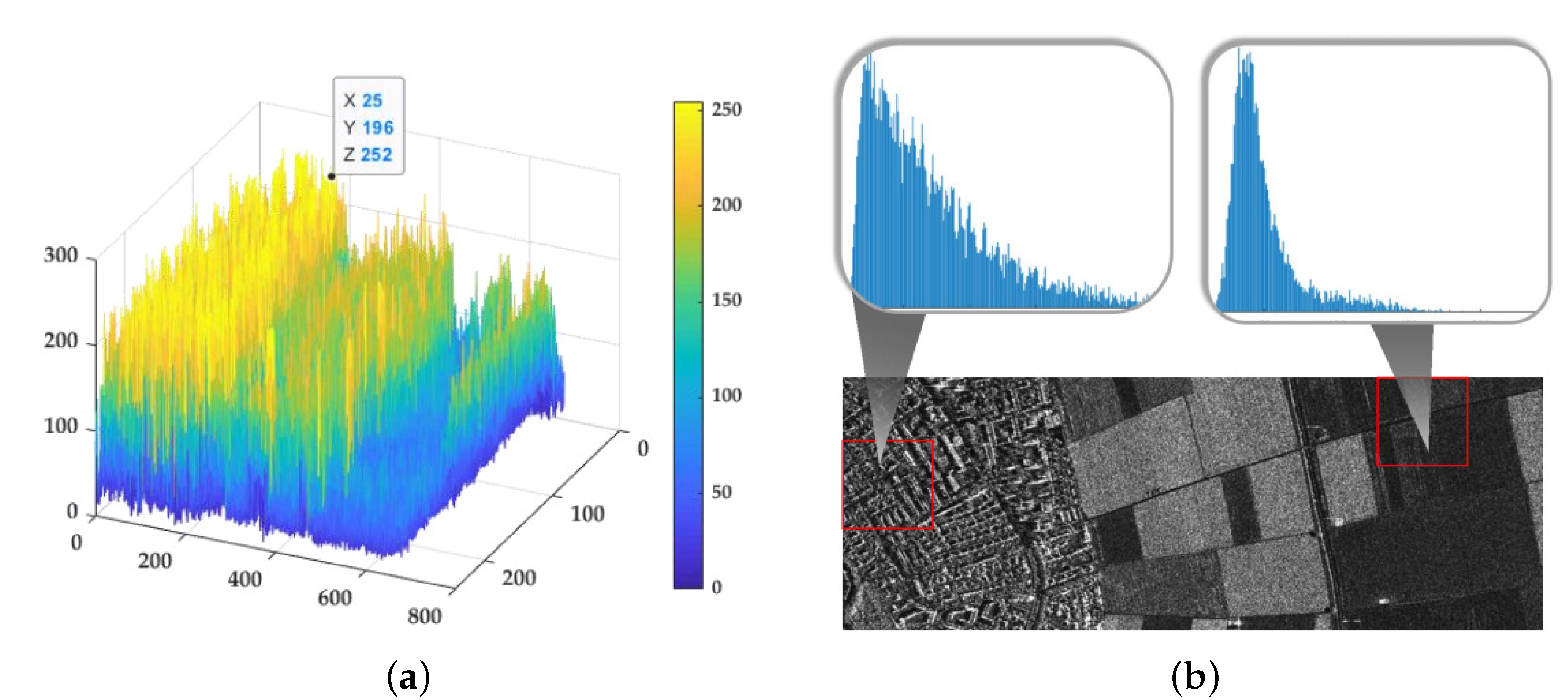
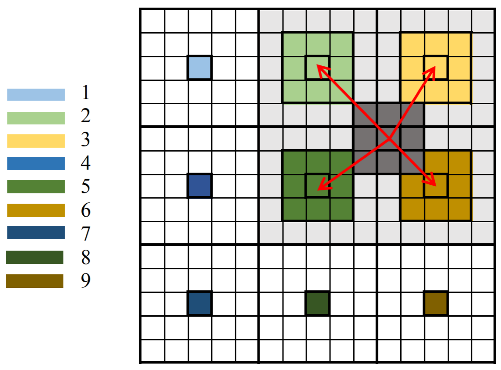
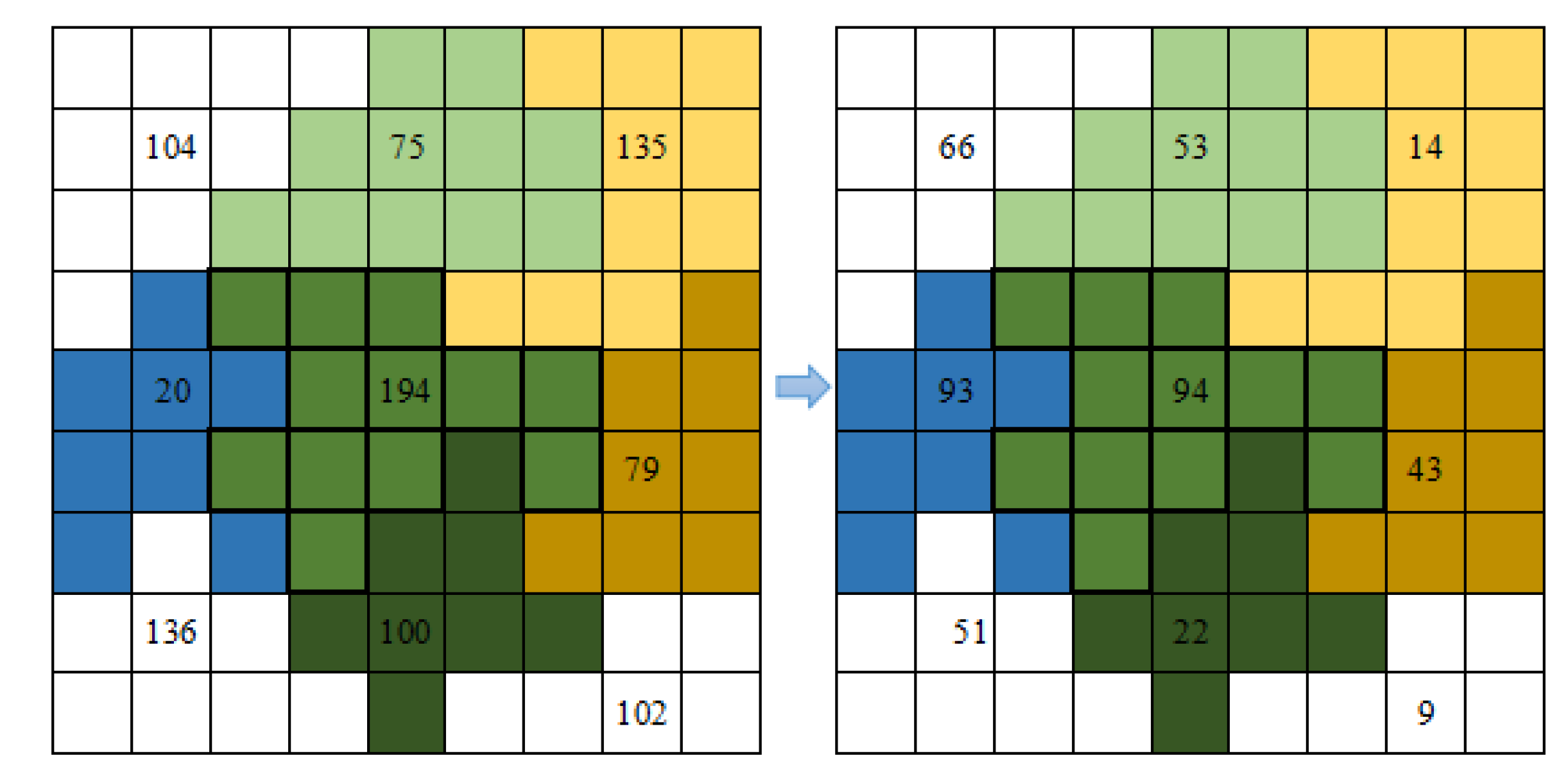
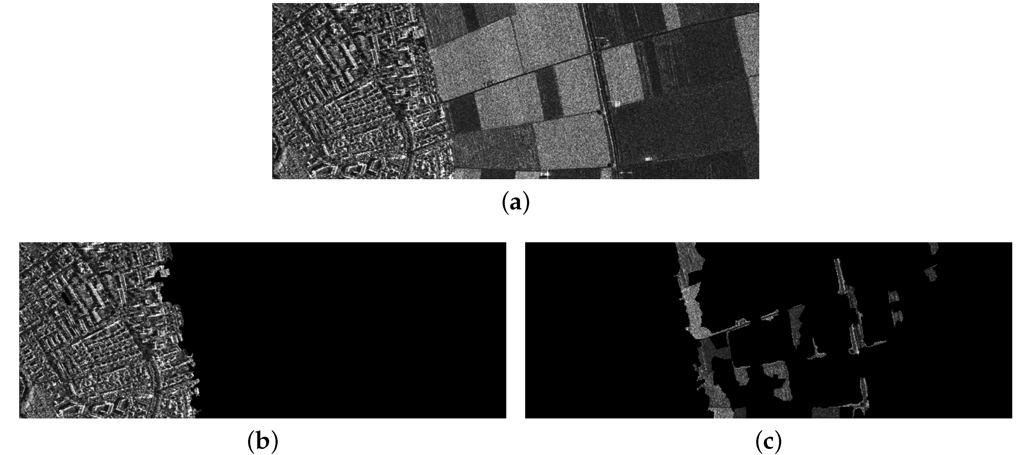
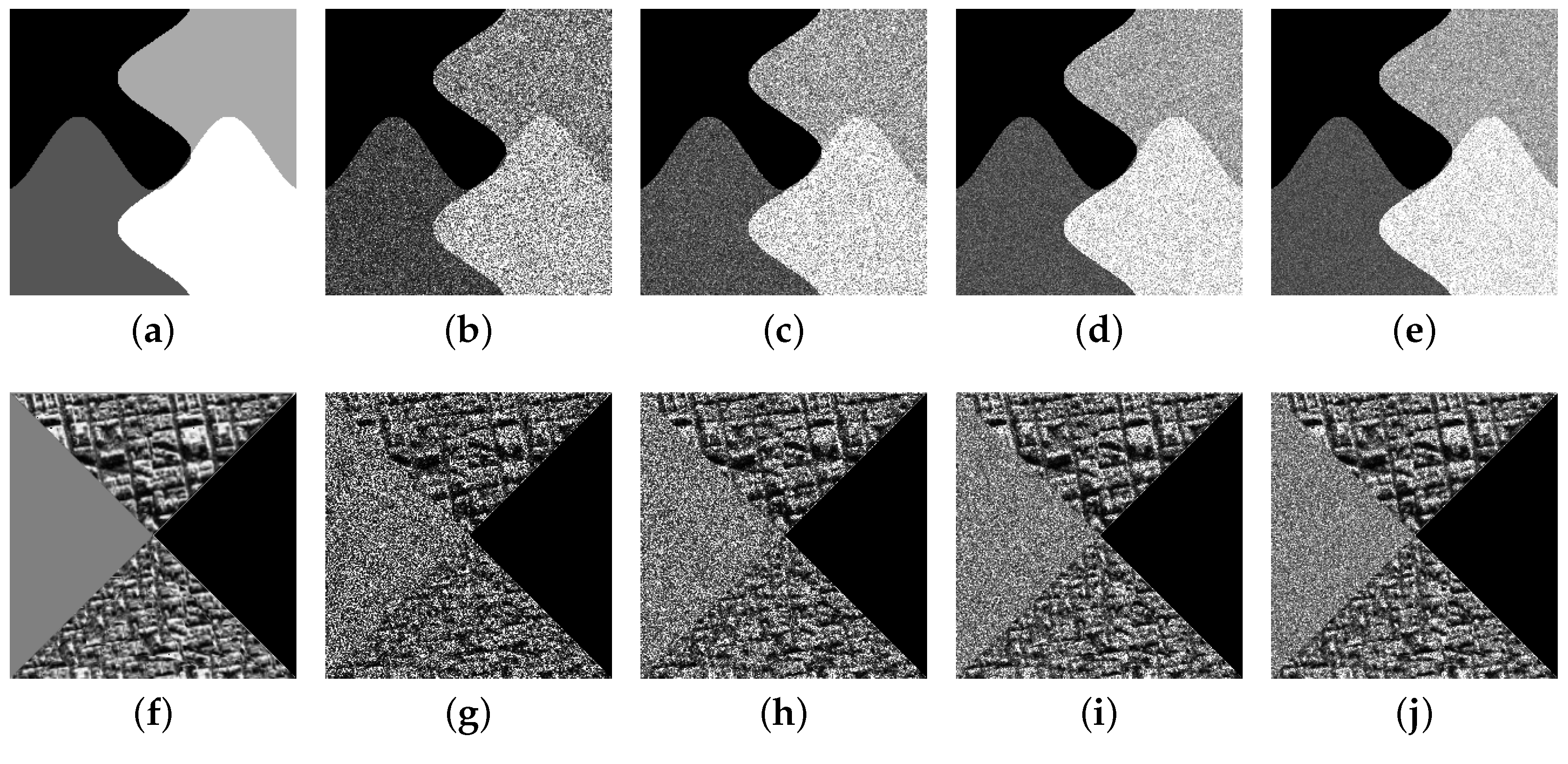
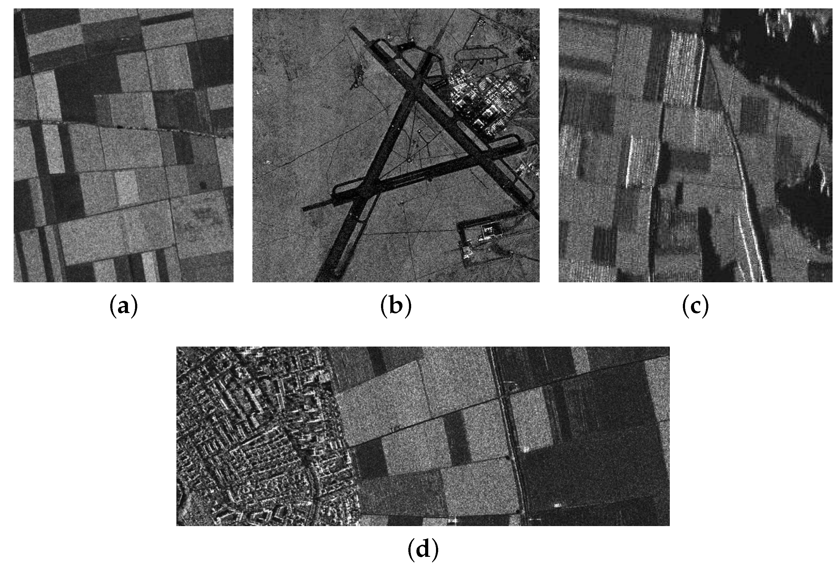
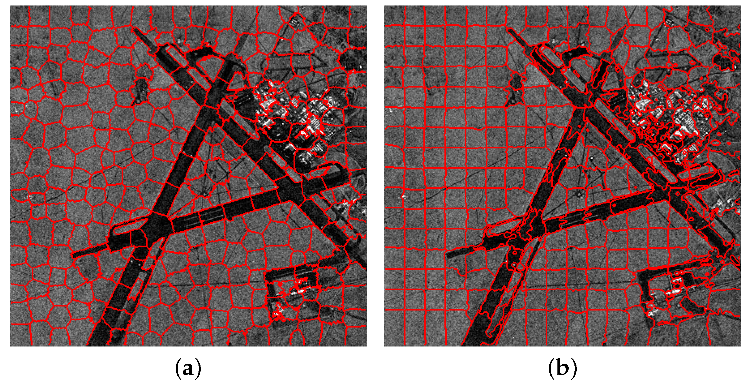
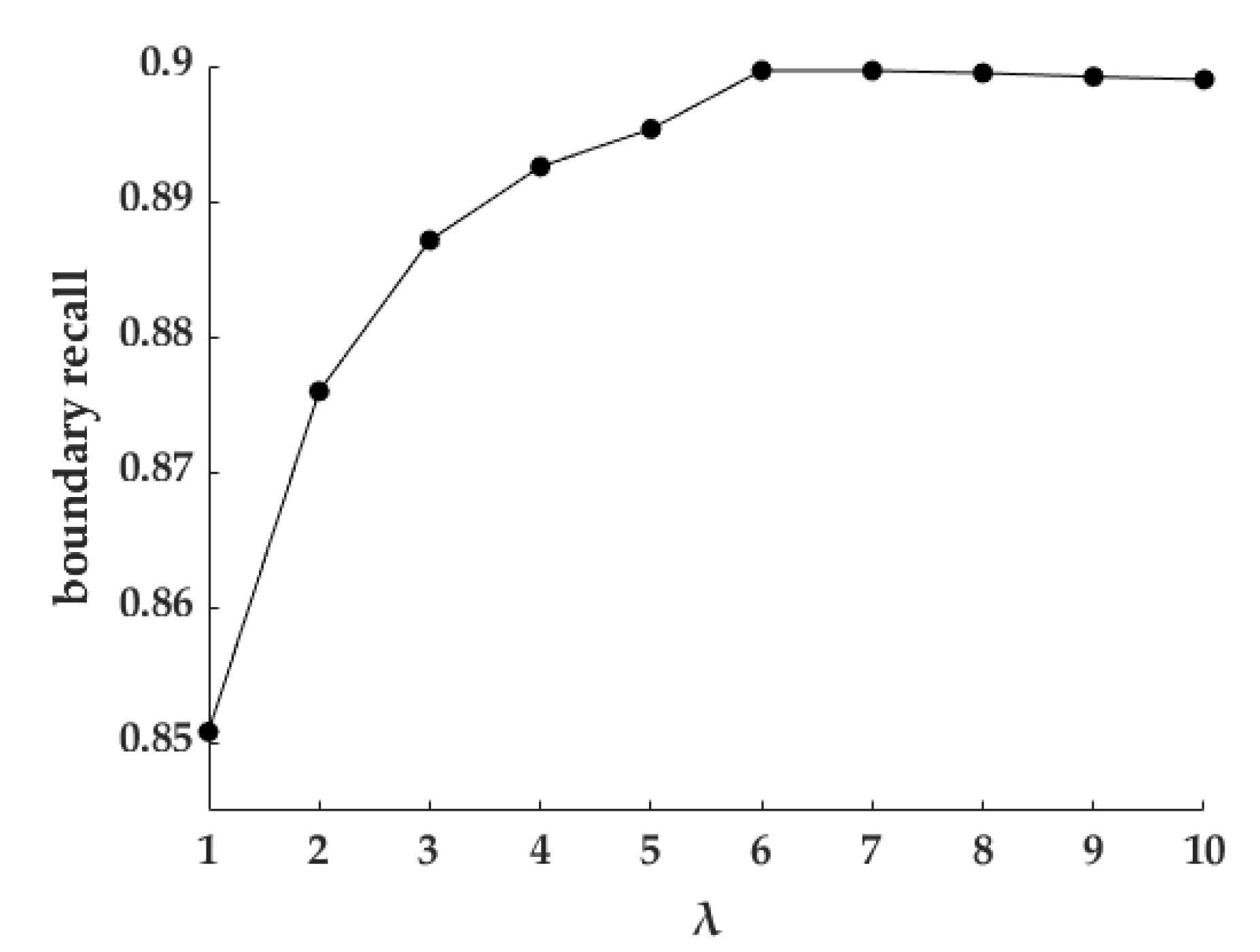
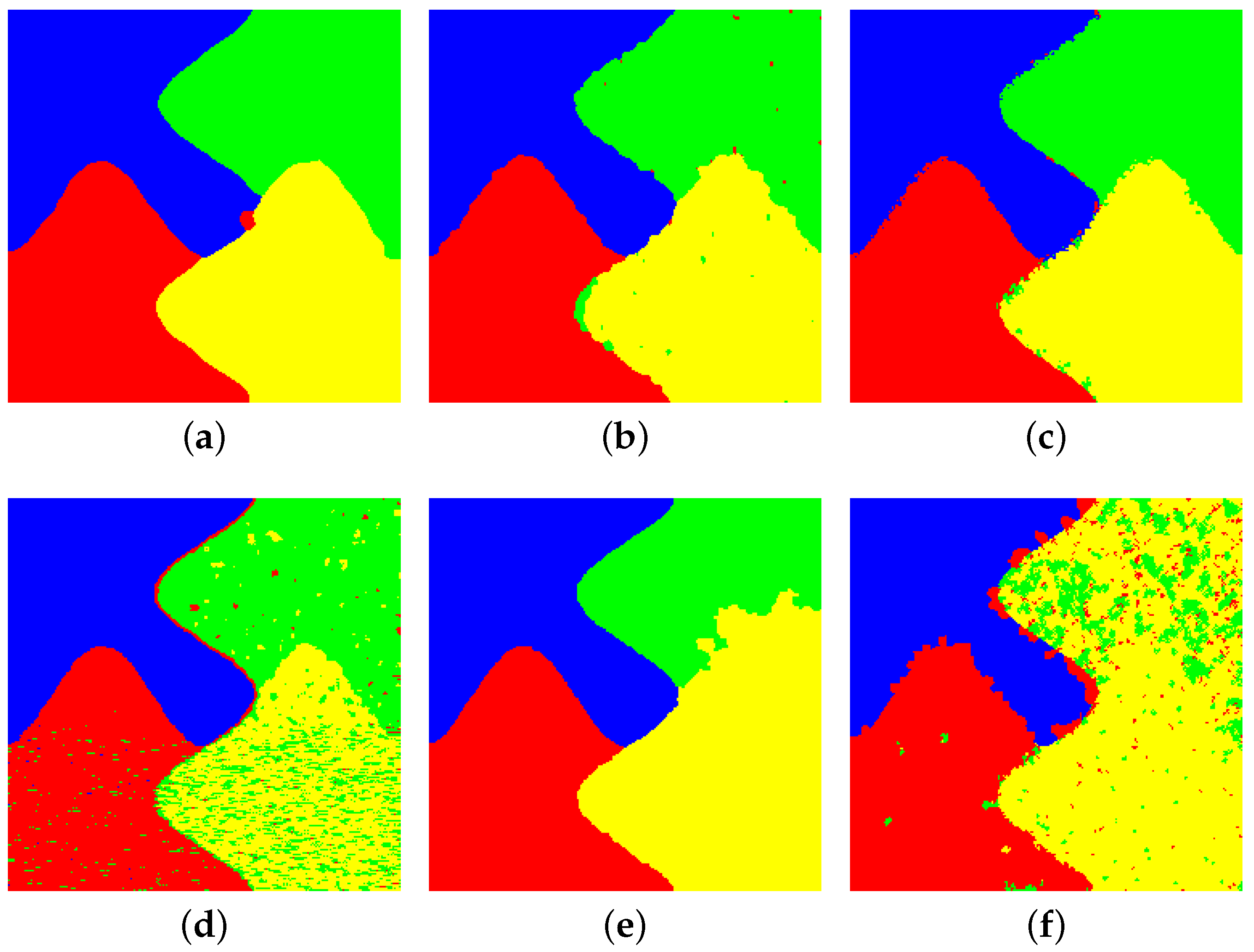
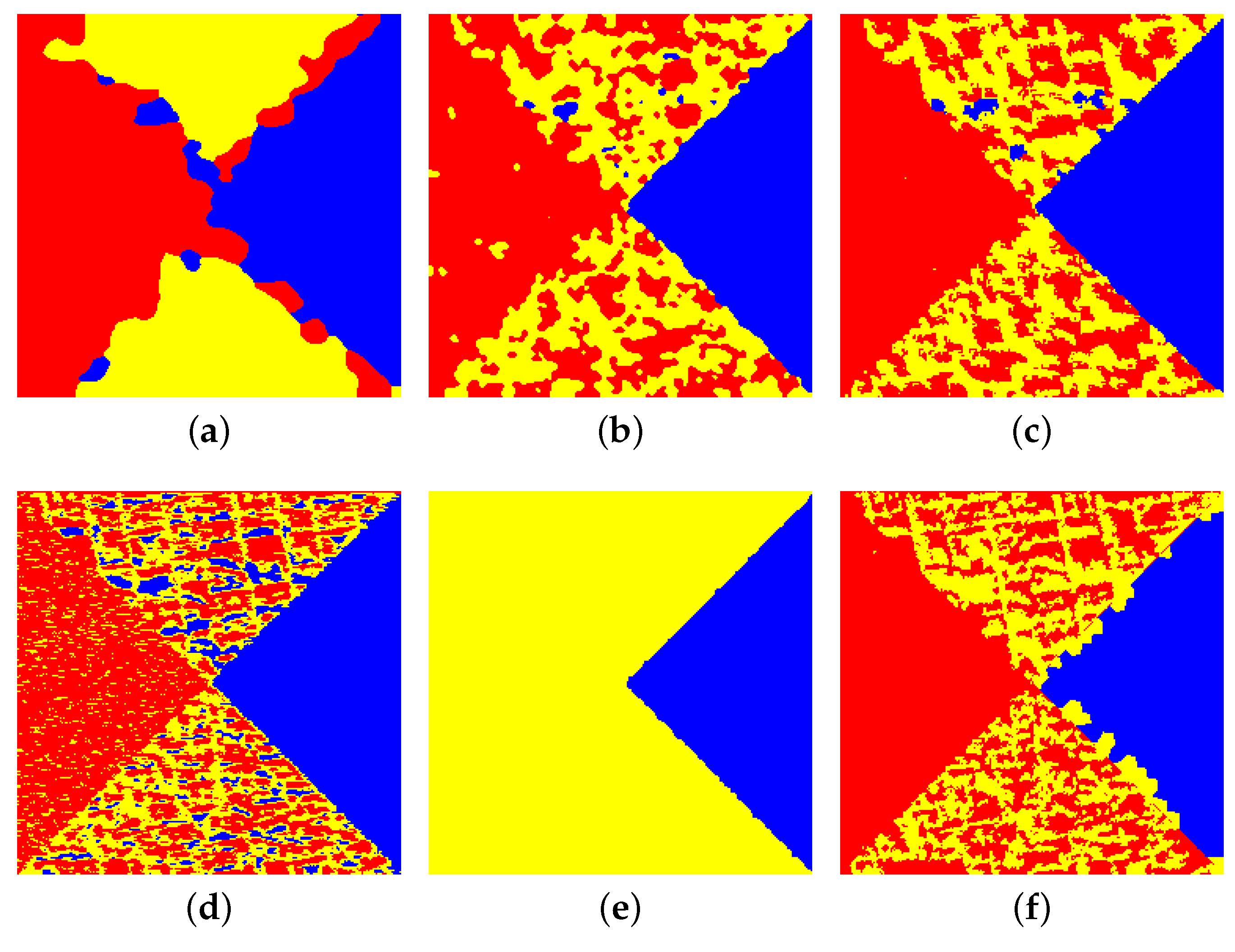
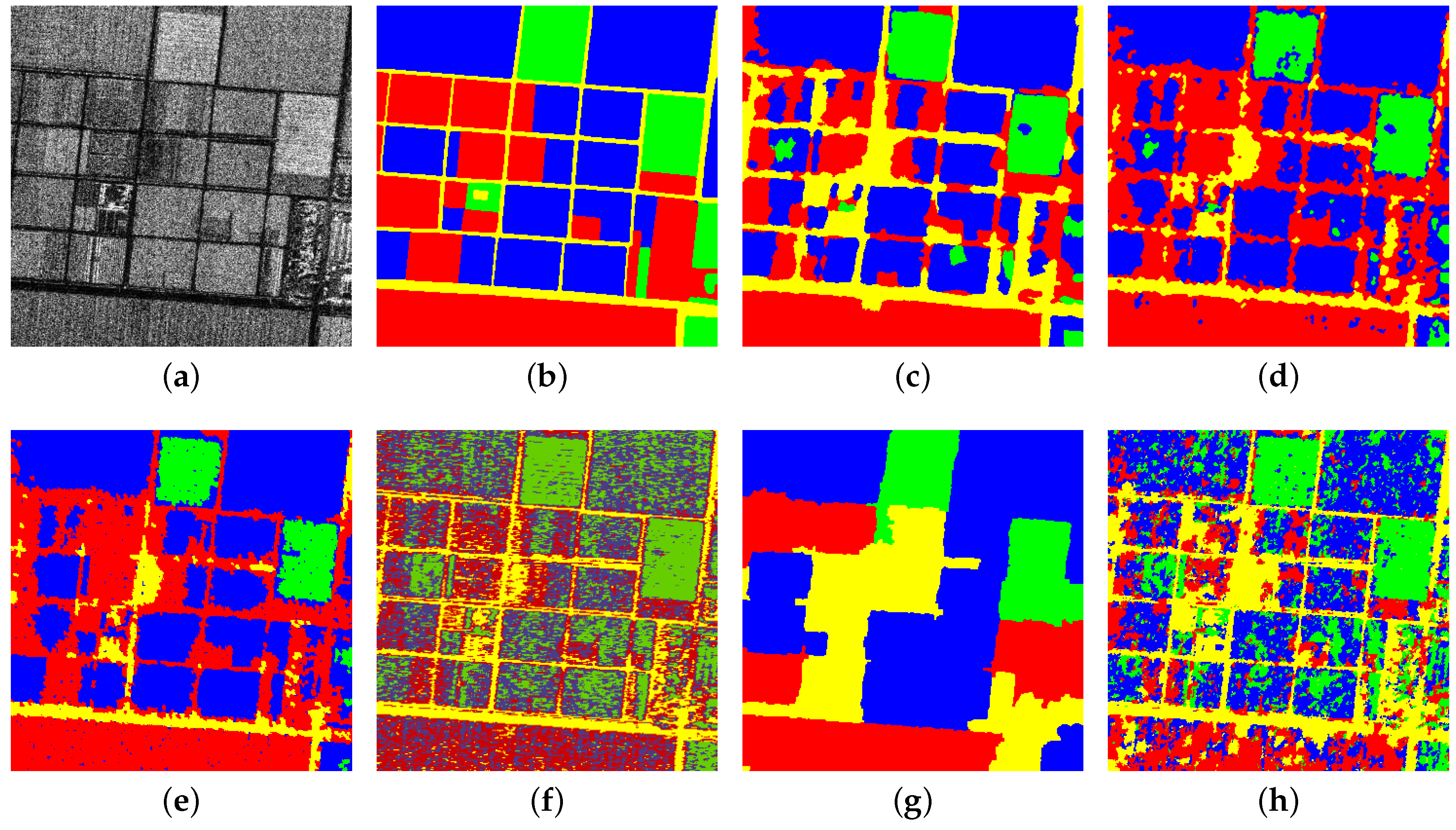
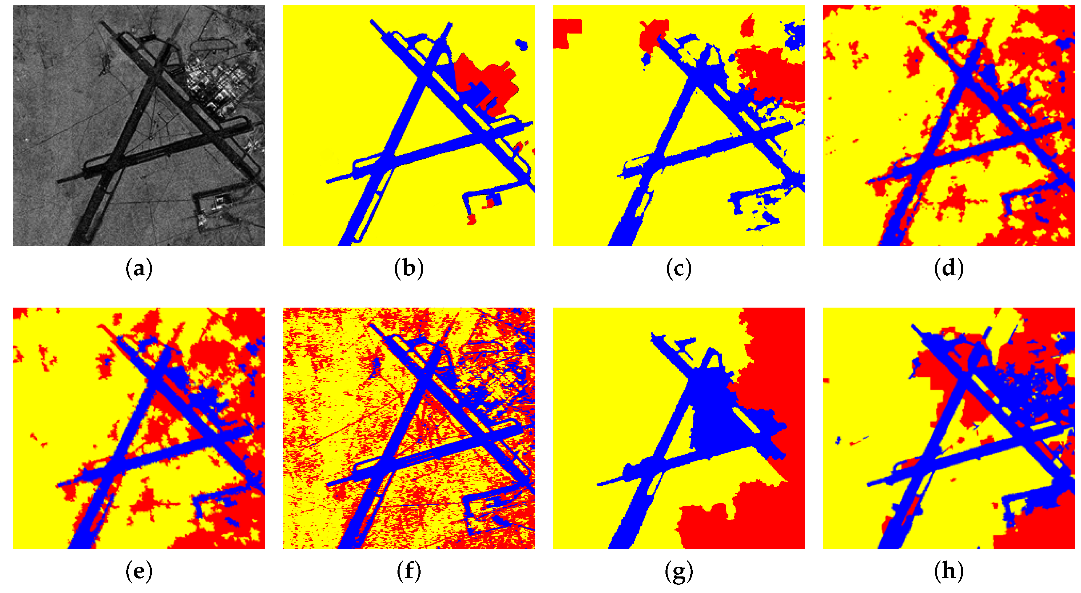
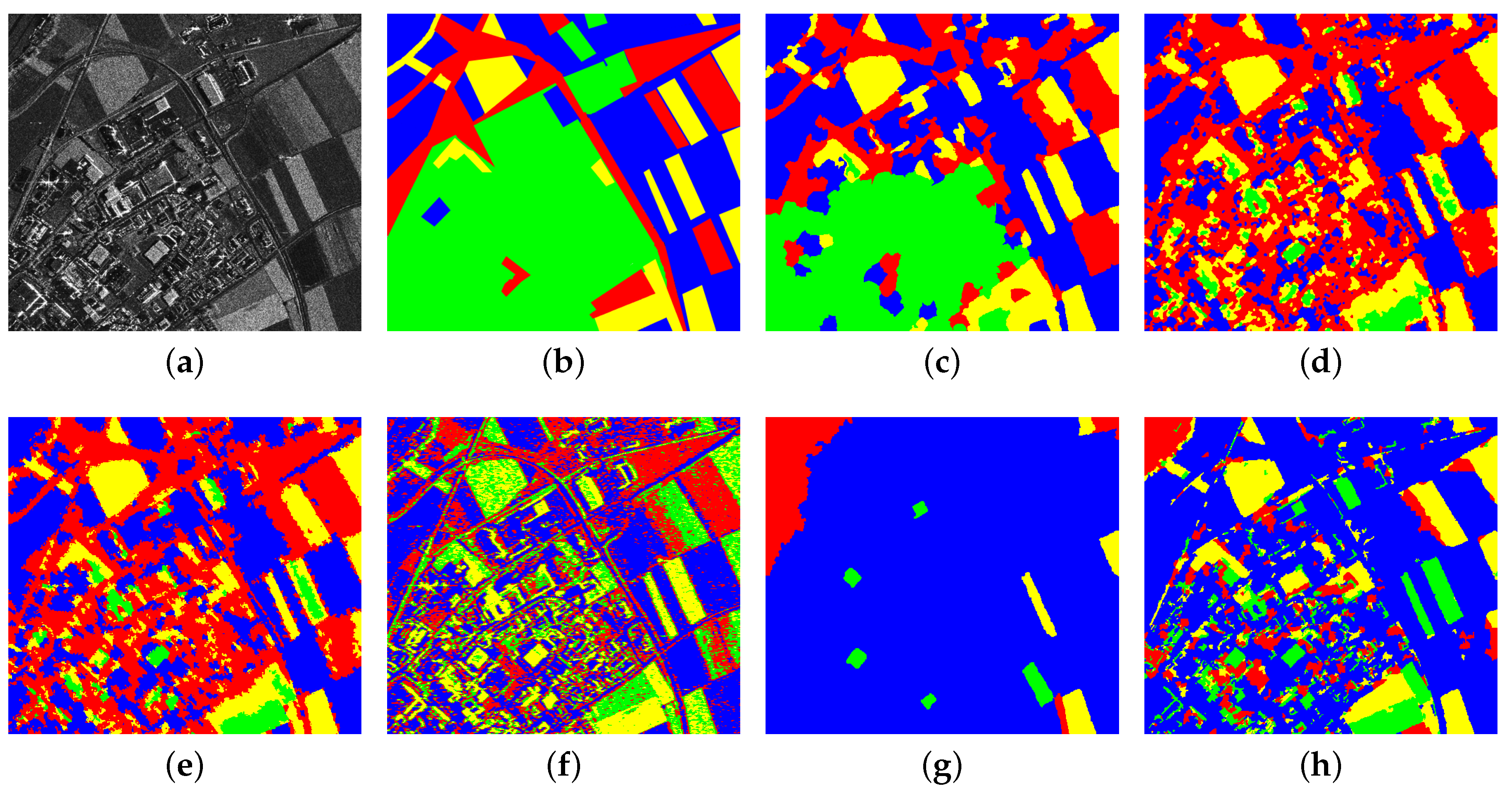
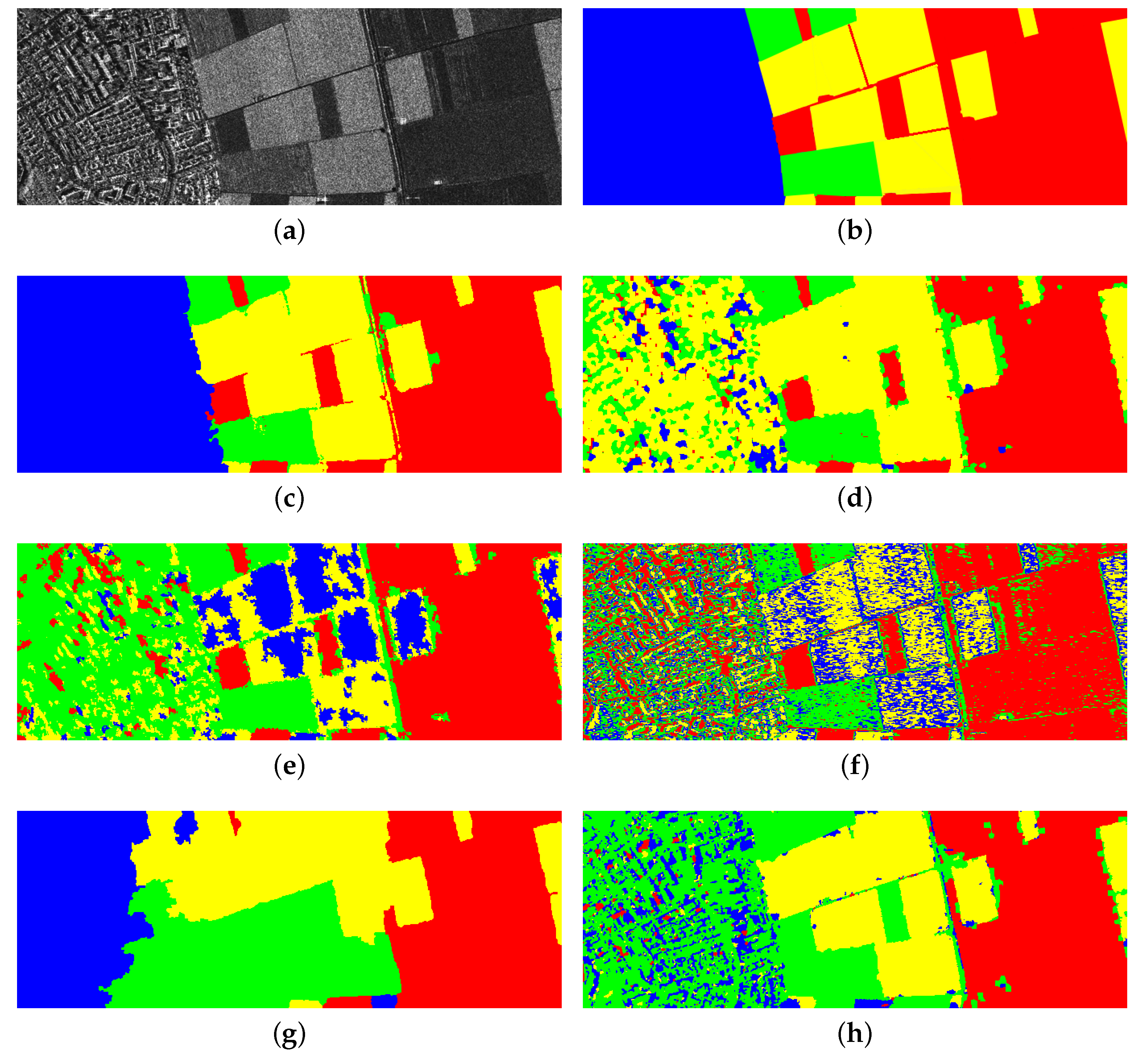
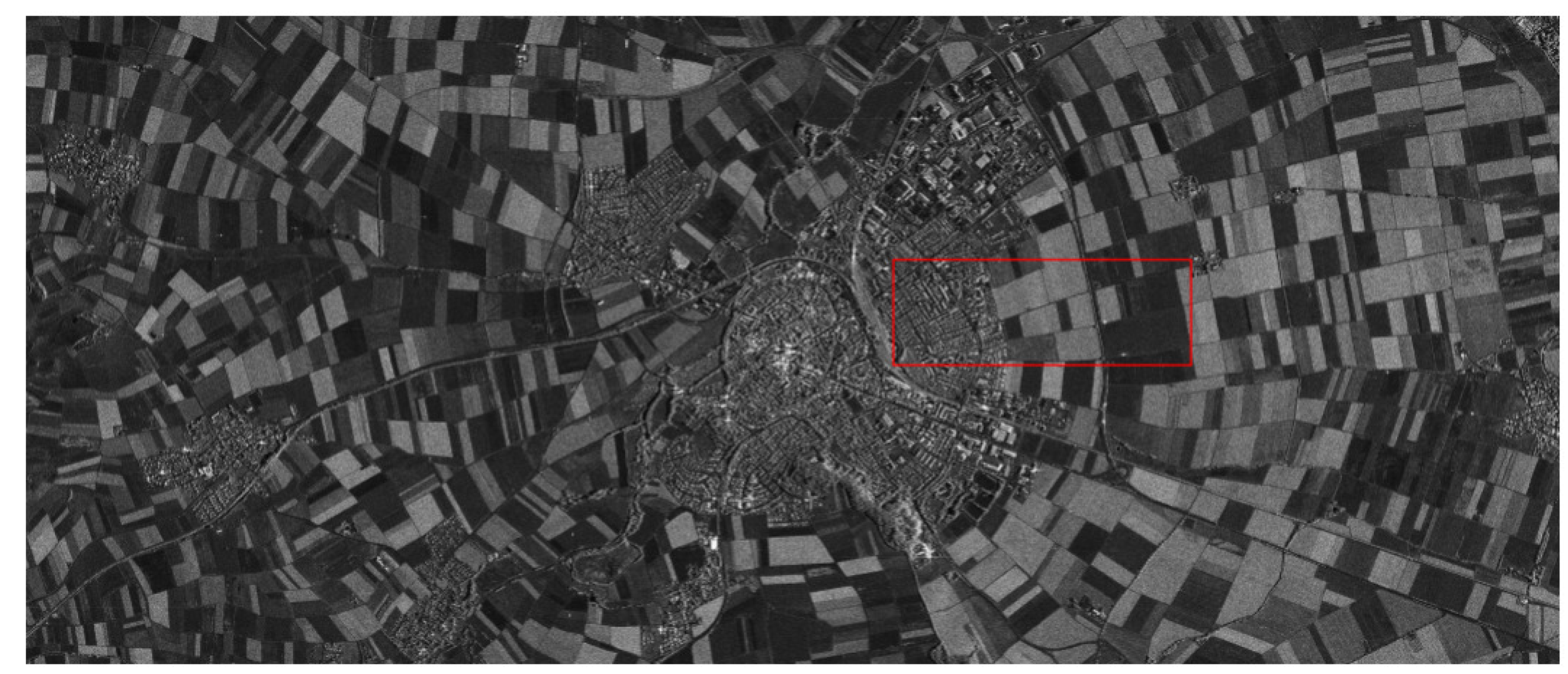
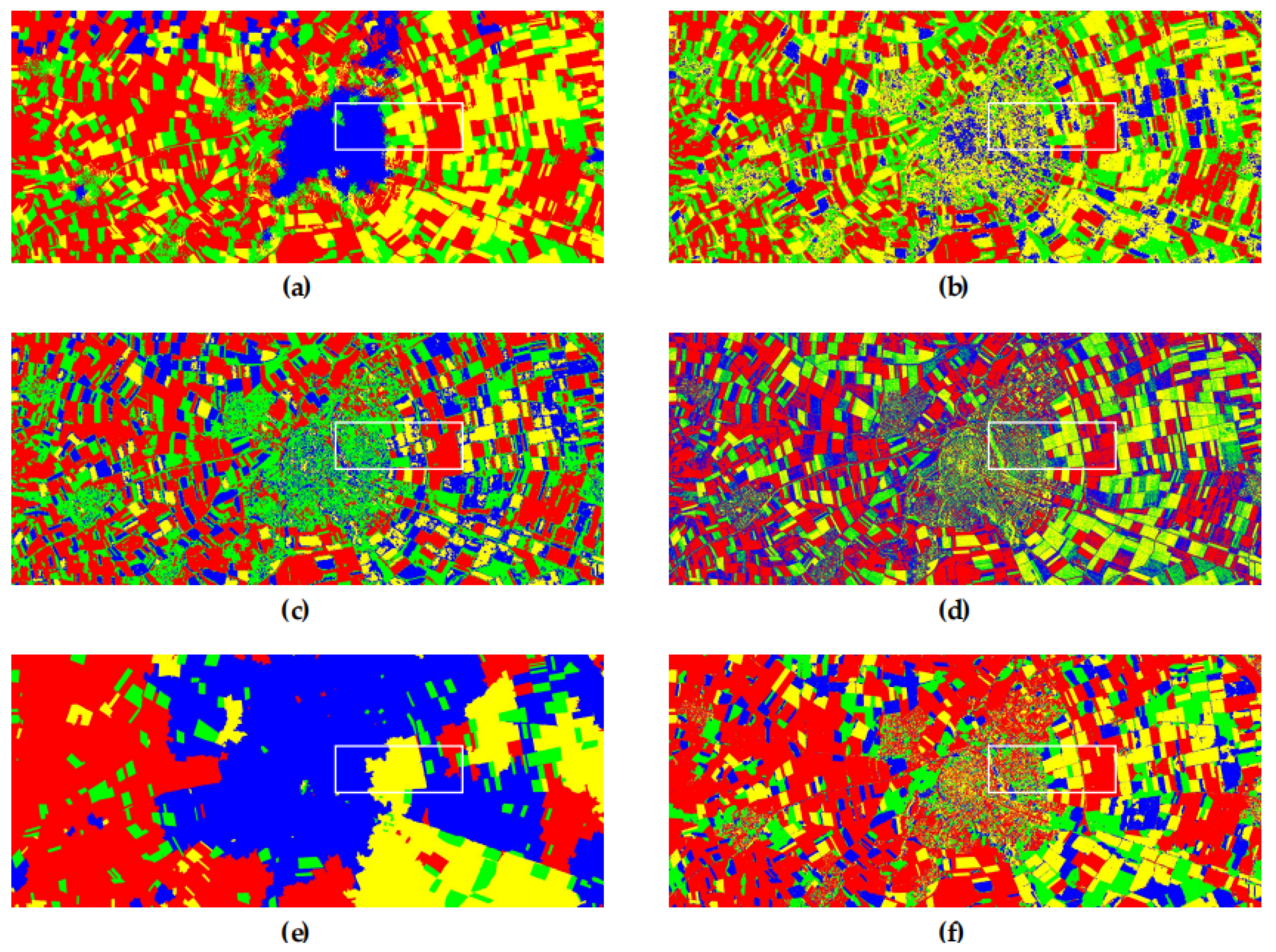
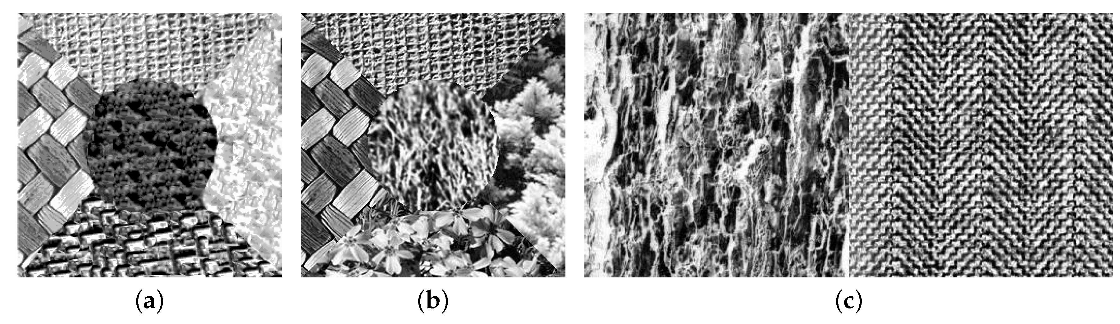
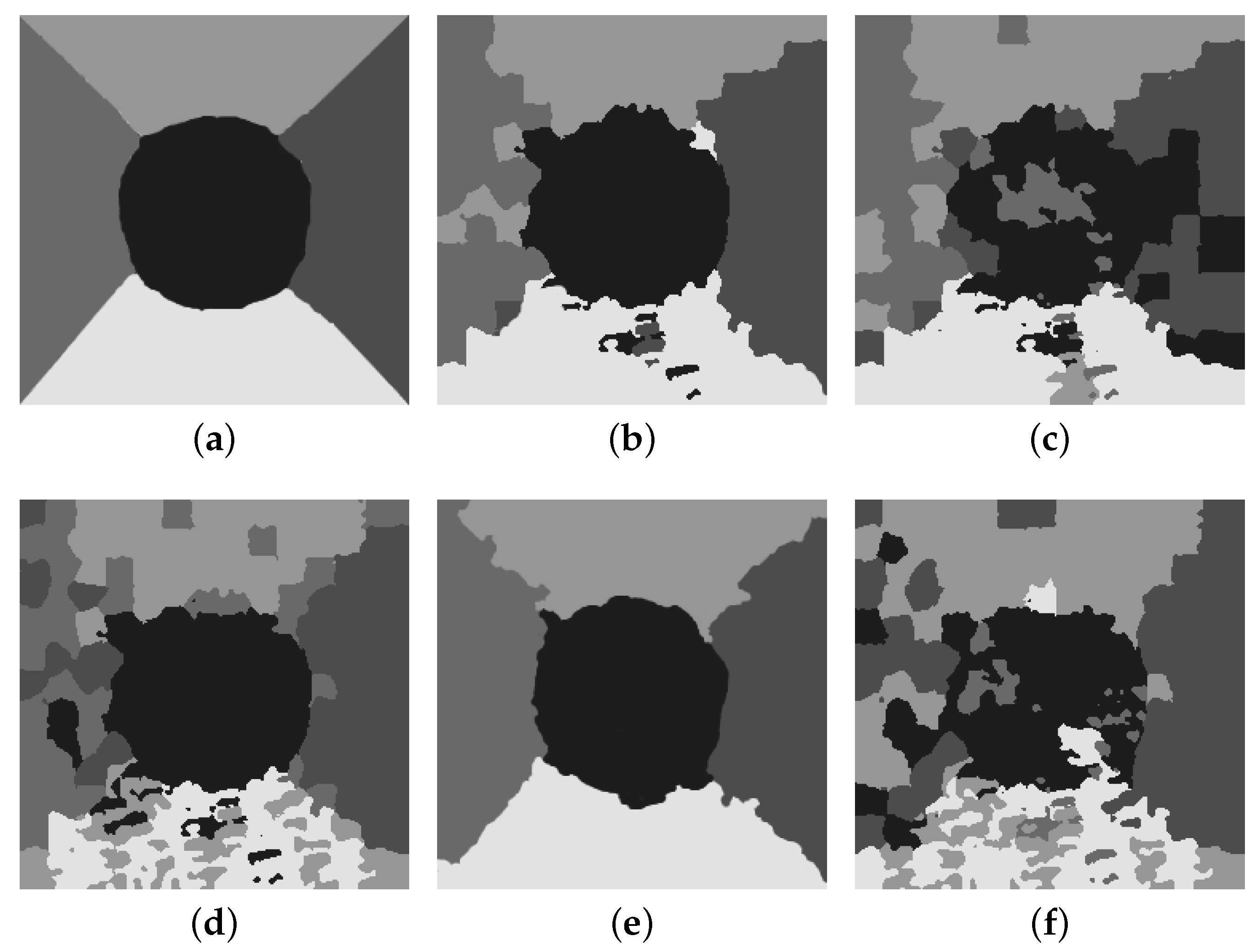
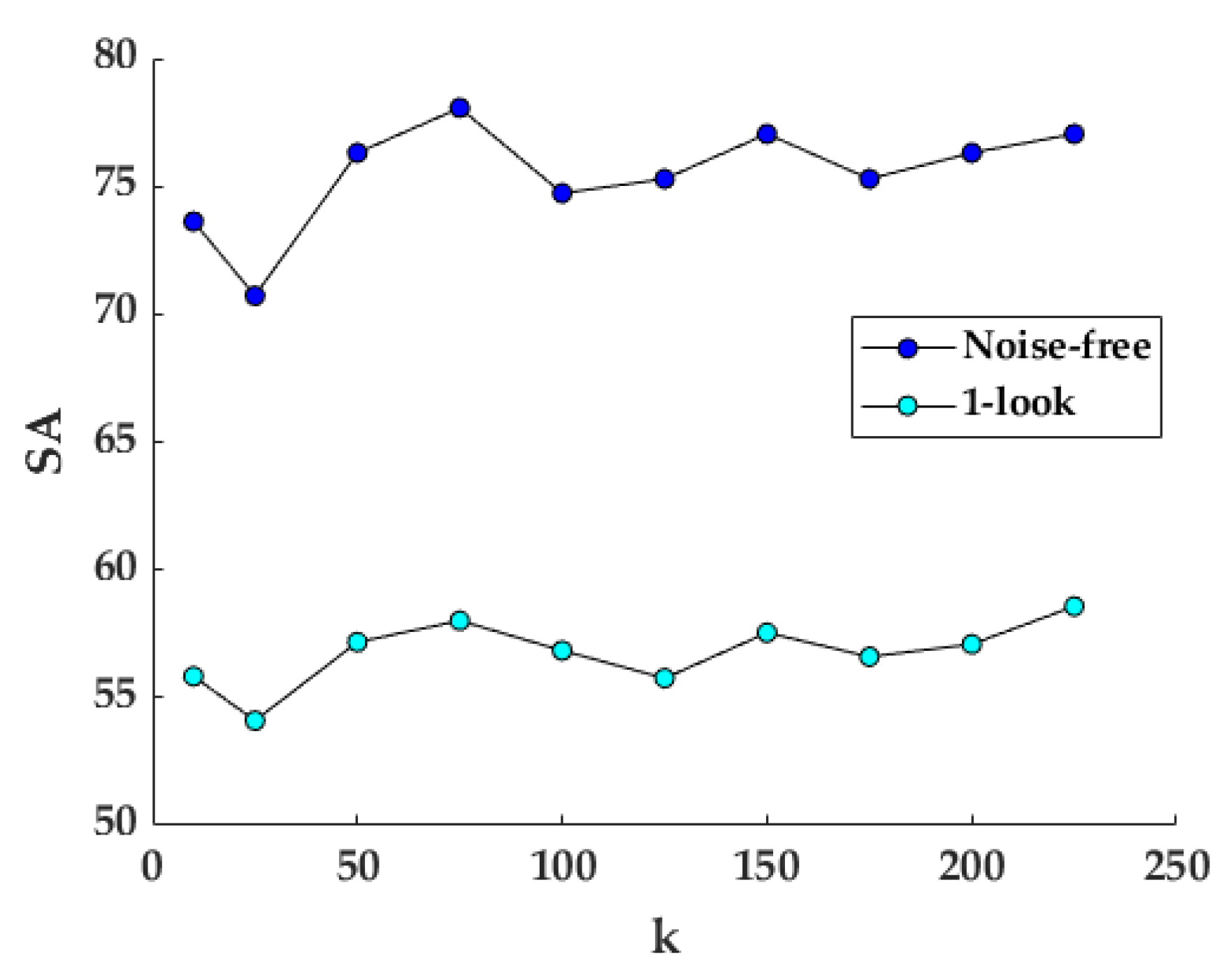
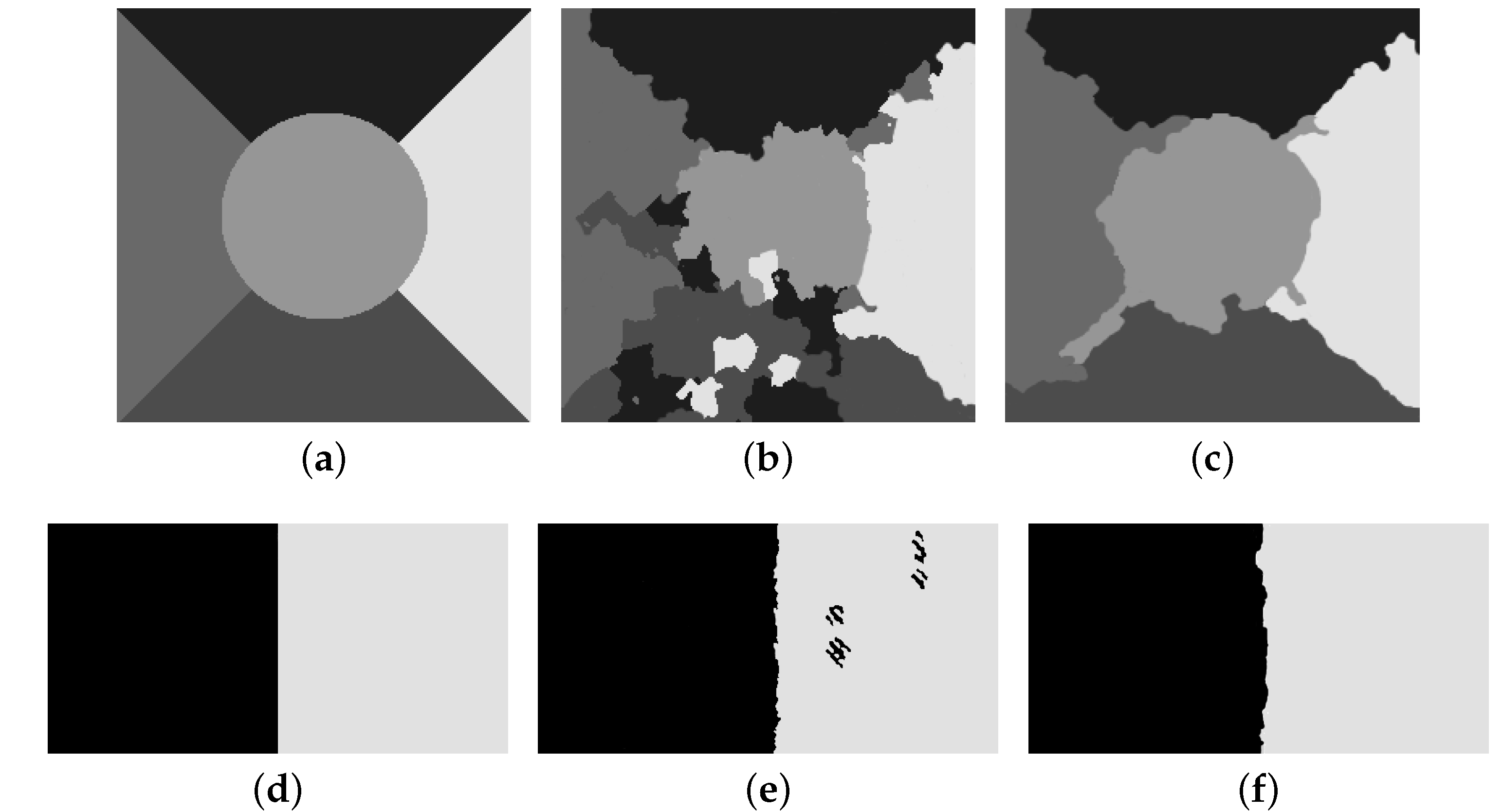
Table 1.
The information of real SAR images.
| Name | Landform | Location | Sensor | Modalities | Polarization |
|---|---|---|---|---|---|
| Maricopa (Figure 8a) | Crops, water | Maricopa | Airborne SAR | StripMap | - |
| Chinalake (Figure 8b) | Buildings, farms, run way | California | UAVSAR | StripMap | - |
| Terracut (Figure 8c) | Crops, buildings | Swabian Jura | TerraSAR | High resolution spotlight | HH |
| Ries (Figure 8d) | Crops, buildings | Swabian Jura | TerraSAR | High resolution spotlight | HH |
Table 2.
Experimental results on SI1 simulated images (%).
| Algorithms | 1-look | 2-look | 4-look | 6-look |
|---|---|---|---|---|
| CKS_FCM [14] | 91.74 | 95.96 | 98.00 | 98.69 |
| FKP_FCM [16] | 98.21 | 98.60 | 98.80 | 99.22 |
| THFCM [43] | 97.25 | 98.49 | 98.81 | 98.90 |
| SFFCM [44] | 93.99 | 94.64 | 99.42 | 99.45 |
| FWCRF [45] | 79.33 | 93.61 | 92.64 | 94.87 |
| TKSFCM | 98.66 | 99.02 | 99.16 | 99.57 |
Table 3.
Experimental results on SI2 simulated images (%).
| Algorithms | 1-look | 2-look | 4-look | 6-look |
|---|---|---|---|---|
| CKS_FCM [14] | 63.36 | 64.32 | 65.95 | 68.50 |
| FKP_FCM [16] | 74.71 | 75.22 | 75.57 | 75.85 |
| THFCM [43] | 74.44 | 75.21 | 74.79 | 75.18 |
| SFFCM [44] | 72.35 | 72.56 | 72.81 | 72.92 |
| FWCRF [45] | 46.22 | 61.14 | 68.30 | 71.68 |
| TKSFCM | 68.82 | 76.84 | 79.63 | 81.15 |
Table 4.
Experimental results on real SAR images (%).
| Algorithms | Maricopa | Chinalake | Terracut | Ries | ||||
|---|---|---|---|---|---|---|---|---|
| SA | F1 | SA | F1 | SA | F1 | SA | F1 | |
| CKS_FCM [14] | 62.49 | 62.99 | 48.05 | 45.04 | 41.39 | 42.77 | 55.05 | 52.15 |
| FKP_FCM [16] | 72.49 | 61.03 | 72.15 | 68.30 | 41.63 | 42.22 | 61.48 | 56.34 |
| THFCM [43] | 79.57 | 78.58 | 71.99 | 68.59 | 42.18 | 43.10 | 48.21 | 44.26 |
| SFFCM [44] | 37.24 | 23.44 | 66.46 | 61.04 | 25.76 | 18.89 | 68.91 | 64.28 |
| FWCRf [45] | 45.01 | 53.54 | 56.20 | 54.71 | 38.49 | 35.54 | 64.21 | 62.27 |
| TKSFCM | 80.91 | 77.69 | 72.58 | 70.93 | 67.64 | 67.60 | 94.27 | 93.56 |
Table 5.
Edge segmentation results (%) of the Maricopa image.
| Algorithms | F1-Score | |||
|---|---|---|---|---|
| CKS_FCM [14] | 55.44 | 58.13 | 50.87 | 67.81 |
| FKP_FCM [16] | 68.30 | 49.20 | 54.93 | 44.55 |
| THFCM [43] | 68.59 | 43.17 | 56.65 | 34.88 |
| SFFCM [44] | 61.04 | 26.60 | 20.81 | 36.88 |
| FWCRF [45] | 54.71 | 51.69 | 38.44 | 78.88 |
| TKSFCM | 70.93 | 55.33 | 43.54 | 75.90 |
Table 6.
Time consumption of algorithms at Terra image.
| Algorithms | CKS_FCM [14] | FKP_FCM [16] | THFCM [43] | SFFCM [44] | FWCRF [45] | TKSFCM |
|---|---|---|---|---|---|---|
| Time | 5 h | 1.7 h | 785 s | 159 s | 873 s | 158 s |
Table 7.
Experimental results on SI3 simulated images (%).
| Algorithms | 1-look | 2-look | 4-look | 6-look | Noise-Free | Noise-Free Minus 1-look |
|---|---|---|---|---|---|---|
| LBP [48] | 41.33 | 51.42 | 55.83 | 58.54 | 73.05 | 31.72 |
| GLCM-h | 40.73 | 46.12 | 49.01 | 53.29 | 72.62 | 31.29 |
| WVN [49] | 60.57 | 64.97 | 69.25 | 79.18 | 92.05 | 33.48 |
| MNN [9] | 44.18 | 46.85 | 49.62 | 59.65 | 72.32 | 28.14 |
| TKSFCM | 62.27 | 67.35 | 71.88 | 77.14 | 87.69 | 25.42 |
© 2020 by the authors. Licensee MDPI, Basel, Switzerland. This article is an open access article distributed under the terms and conditions of the Creative Commons Attribution (CC BY) license (http://creativecommons.org/licenses/by/4.0/).
Share and Cite
MDPI and ACS Style
Shang, R.; Peng, P.; Shang, F.; Jiao, L.; Shen, Y.; Stolkin, R. Semantic Segmentation for SAR Image Based on Texture Complexity Analysis and Key Superpixels. Remote Sens. 2020, 12, 2141. https://doi.org/10.3390/rs12132141
AMA Style
Shang R, Peng P, Shang F, Jiao L, Shen Y, Stolkin R. Semantic Segmentation for SAR Image Based on Texture Complexity Analysis and Key Superpixels. Remote Sensing. 2020; 12(13):2141. https://doi.org/10.3390/rs12132141
Chicago/Turabian StyleShang, Ronghua, Pei Peng, Fanhua Shang, Licheng Jiao, Yifei Shen, and Rustam Stolkin. 2020. "Semantic Segmentation for SAR Image Based on Texture Complexity Analysis and Key Superpixels" Remote Sensing 12, no. 13: 2141. https://doi.org/10.3390/rs12132141
Note that from the first issue of 2016, this journal uses article numbers instead of page numbers. See further details here.