Modeling and Validation of the Cool Summer Microclimate Formed by Passive Cooling Elements in a Semi-Outdoor Building Space

1
Department of Architecture and Building Engineering, Tokyo Institute of Technology, 4259 Nagatsuta-cho, Midori-ku, Yokohama, Kanagawa 226-8502, Japan
2
Misawa Homes Institute of Research and Development, 1-1-19, Takaidonishi, Suginami-ku, Tokyo 168-0071, Japan
*
Author to whom correspondence should be addressed.
Sustainability 2020, 12(13), 5360; https://doi.org/10.3390/su12135360
Submission received: 27 May 2020
/
Revised: 29 June 2020
/
Accepted: 30 June 2020
/
Published: 2 July 2020
Abstract
:Previous measurements (Del Rio et al. 2019) have confirmed the formation of cool summer microclimates through a combination of passive cooling elements (i.e., evaporative cooling louver, vegetation, and sunscreen) in semi-outdoor building spaces in Japan. Computational fluid dynamics (CFD) simulation is useful to understand the contribution of each element to semi-outdoor and indoor microclimates with natural ventilation, and to determine their effective combination. To date, there have not been sufficient studies on the modeling and validation for the CFD simulation of microclimates by such elements. This study demonstrates the modeling method using literature-based values and field measurements. It also demonstrates model validity by comparing the obtained results with field measurements. The results show that CFD simulation with detailed modeling of these elements can replicate vertical temperature distributions at four different positions across the semi-outdoor space and indoor space. The maximum difference in air temperature between the measurements and simulation results was 0.7–1 °C. The sensitivities of each passive cooling element on the microclimates formed in both spaces were confirmed. The watered louver condition and shorter louver–window distance were most effective in cooling both spaces. These results indicate that the modeling method could be effectively applied to assess cool microclimates and formulate a passive cooling design.
1. Introduction
Building microclimates have a strong influence on the effectiveness of natural ventilation [1,2,3,4,5]. In the hot humid summer climate of Tokyo, a combination of factors such as reduced green spaces and increasingly compact house design in urban and suburban areas has made it difficult to maintain a comfortable indoor environment using only passive cooling methods such as natural ventilation and solar shading. Moreover, alternating natural and artificial ground covers have a reduced capacity to retain water, attenuating the cooling effect of evaporation from the ground [6]. As a result, building users tend to use air conditioners instead of natural ventilation to maintain a comfortable indoor thermal environment [7]. However, the continuous use of air conditioners increases energy consumption [7], and anthropogenic heat negatively impacts the outdoor thermal environment. This highlights the importance of the design of sustainable and comfortable urban spaces and buildings [8].
The use of passive cooling methods [9,10] in cities and residential areas is an adaptive measure for severe thermal environments. The planting of trees and green cover is one of the most effective ways to improve the urban thermal environment [9,10]. In reality, it is difficult to achieve an objective cooling effect due to the limited amount of green spaces in compact urban areas. As such, alternative solutions that combine multiple passive cooling methods are required to improve the microclimate of compact urban spaces. The development of practical passive cooling methods has been studied extensively in Japan [4,11,12,13,14]. Direct evaporative cooling is the simplest and oldest form of air conditioning [10]; these systems are dependent on climatic conditions. Although they are expected to be more effective in hot and dry climates, studies [15,16] have shown that they can also function in hot and humid climates. The use of evaporative cooling is a widely used passive cooling method in traditional Japanese vernacular houses [17]. The summer season in Japan is characterized by hot and humid weather with abundant rainfall; however, the relative humidity decreases to approximately 50% during the daytime on sunny days. Therefore, evaporative cooling has the potential to improve the microclimate during the hot daytime hours in Japan. Hirayama et al. [12] developed an evaporative cooling louver that lowers air temperature by a maximum of approximately 3.0 °C within the vicinity of the louver. The louver is a stand-alone aluminum louver system coated with hydrophilic resin, porous particles, and a photocatalyst (TiO2) that disperses water over the entire surface using only a small amount of water. The louver is sufficiently wet with the continuous drip of water from the top of the louver, which then evaporates, cooling the air that flows easily through the slats. The louver provides (1) shade against direct solar radiation, (2) radiation cooling, (3) ventilation cooling with cooled airflow, and (4) privacy near the window. The louver also has an independent foundation (350x350 mm), offering practical applications for its installation in limited outdoor spaces. Even though the louver improves the microclimate within its vicinity, its actual performance inside buildings has not yet been evaluated. Therefore, more information on the cooling effect of the louver, either alone or in combination with other passive cooling methods, is required to provide design recommendations for generating cool microclimates inside buildings.
This study analyzed the generation of a cool microclimate using passive cooling elements (PCEs) in a semi-outdoor space of a residence in one of Japan’s hottest cities—Kumagaya City. The PCEs investigated in this study include the evaporative cooling louver, surrounding vegetation (trees and flower pots), and sunscreens, evaluated using computational fluid dynamics (CFD). Previous measurements [14] have confirmed the formation of cool summer microclimates by combined PCEs in the semi-outdoor space. Computational fluid dynamics (CFD) simulation was useful to compute the contribution and sensitivity of each element on the semi-outdoor and indoor microclimate through natural ventilation, and determine their effective combination. Compared to field measurements conducted at a limited number of points, CFD simulations can provide detailed information on any variable in the entire computational domain (cited by [18]). Once validated, numerical simulations have the advantage of performing comparative analyses based on different scenarios and designs with limited time and cost. However, there has been insufficient modeling and validation of CFD simulation of microclimates formed by PCEs. This study demonstrates the modeling method using literature-based values and field measurements, and proves its validity by comparing it with field measurement results and implementing sensitivity analysis.
2. Literature Review and State of Art
There has been considerable research focusing on urban microclimate modeling and its validation. Microclimates formed by surrounding buildings [19,20], vegetation [21,22], and cool materials [23] have been simulated using numerical models in urban spaces; this enables the assessment of their effects on human thermal comfort [24]. Most microclimate simulations target a specific height around 1–2 m from the ground and discuss the two-dimensional (2D) horizontal distribution of these microclimates. Model validation is only conducted for limited points at a fixed height.
Numerical simulations have been also applied to assess the thermal and energy performance of buildings, including the effects of envelope materials (e.g., wall materials, phase change materials) [25,26,27]. There has also been intensive research into numerical simulations to evaluate the effects of outdoor microclimates on the indoor environment as passive cooling techniques [28]. This includes evaluation of the effects of the outdoor radiation environment on the solar heat gain of buildings [29,30], the outdoor wind environment on the natural ventilation of buildings [2,3,5], the outdoor microclimate on building thermal performance [31,32,33] and energy demands [34,35,36,37,38,39,40], and outdoor overheating, including urban heat islands, on the energy demand of buildings [41,42]. In particular, vegetation models have been applied to numerical simulations to evaluate solar shading [43,44,45,46], wind break [47], and overall cooling effects [48,49] derived from vegetation on the indoor thermal environment. The effects of cool pavements and materials on building energy use and thermal environment have also been evaluated [50,51]. However, there has been limited discussion on the effects of cool microclimates for a spatial scale less than 1 m, with the detailed vertical distribution formed by vegetation and cool materials. Furthermore, the combined effect of multiple elements (e.g., vegetation and cool materials) has received less attention [4,14]. This is primarily due to the complexity of calculating two semi-independent spaces (outdoor and indoor) simultaneously, whilst considering the physical phenomena at the surface and in the vicinity of space components.
Field measurements in a previous study [14] have shown that the spatial scale of the cool microclimate formed by PCEs was less than 1 m, having a characteristic vertical temperature gradient from the ground (i.e., accumulation of cooled air near the ground) in a semi-outdoor building space. It was suggested that a part of the cool microclimate was induced into the indoor space with natural ventilation through window openings near the space. This measurement could not identify if the characteristic microclimates were formed by the individual effect of PCEs or their combined effect. Identifying primary contributors to the cool microclimate and determining the extent to which they affect the indoor microclimate are important research tasks.
3. Materials and Methods
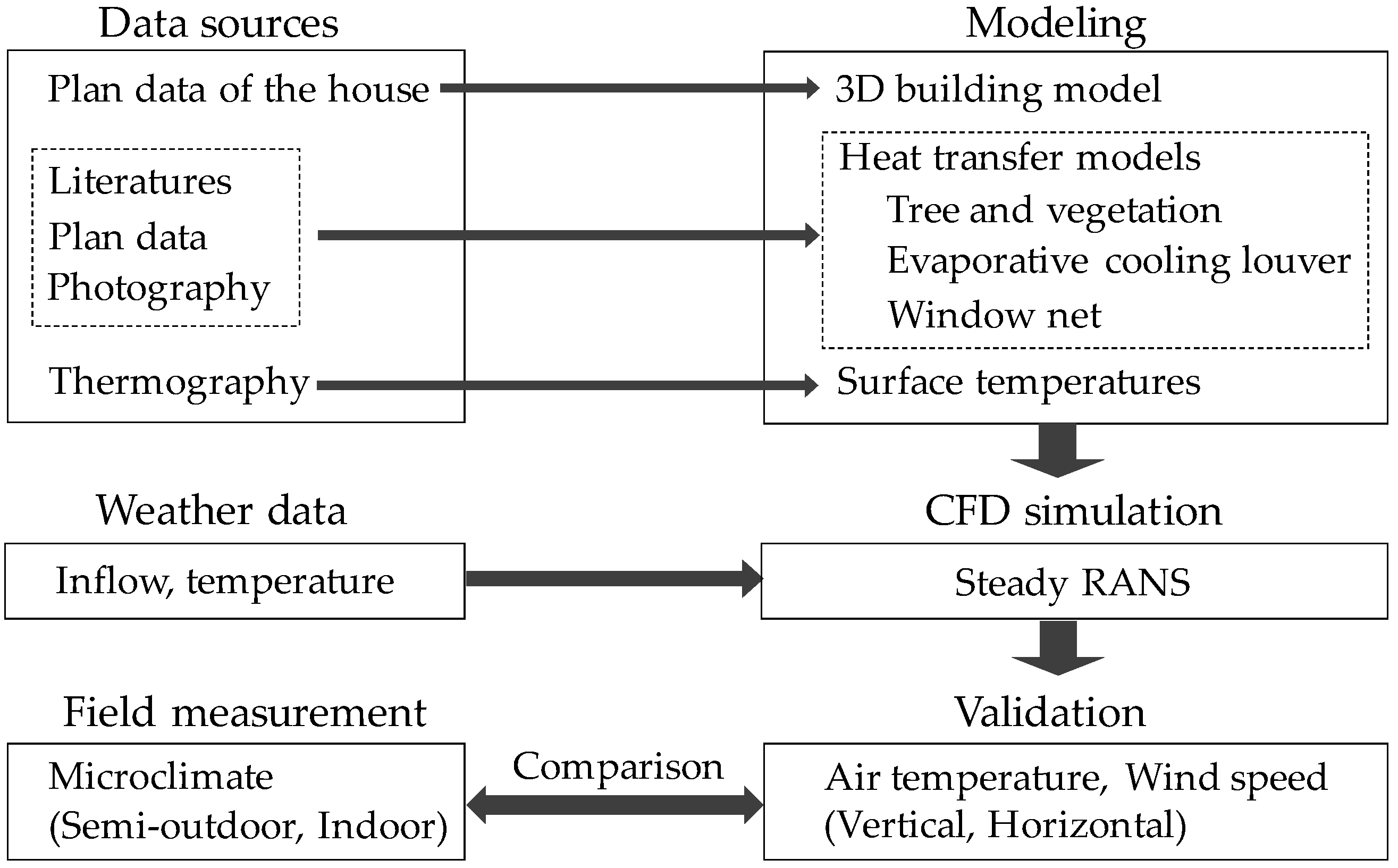
3.1. Method Outline
A CFD model was built using previous field measurement data and introducing heat transfer models of individual PCEs from the literature. The simulation focuses on the flow field, with careful calculation of heat transfer from objects. Field measurement data were used to determine the initial condition and surface temperature of the building materials and ground cover. Moreover, measured microclimate data were used to validate the CFD model by evaluating the synthetic effect of the multiple introduced heat transfer models. A flow chart of the research method is shown in Figure 1. First, a previous field experiment of semi-outdoor and indoor microclimates for a house with multiple PCEs in a semi-outdoor space was described. Second, the modeling details of the PCEs in the semi-outdoor space were explained in relation to the CFD simulation. Third, the results of the CFD simulation were validated using the field experiment results. Finally, a sensitivity analysis of individual and combined effects on PCEs was conducted using the validated CFD simulation.
3.2. Field Measurement
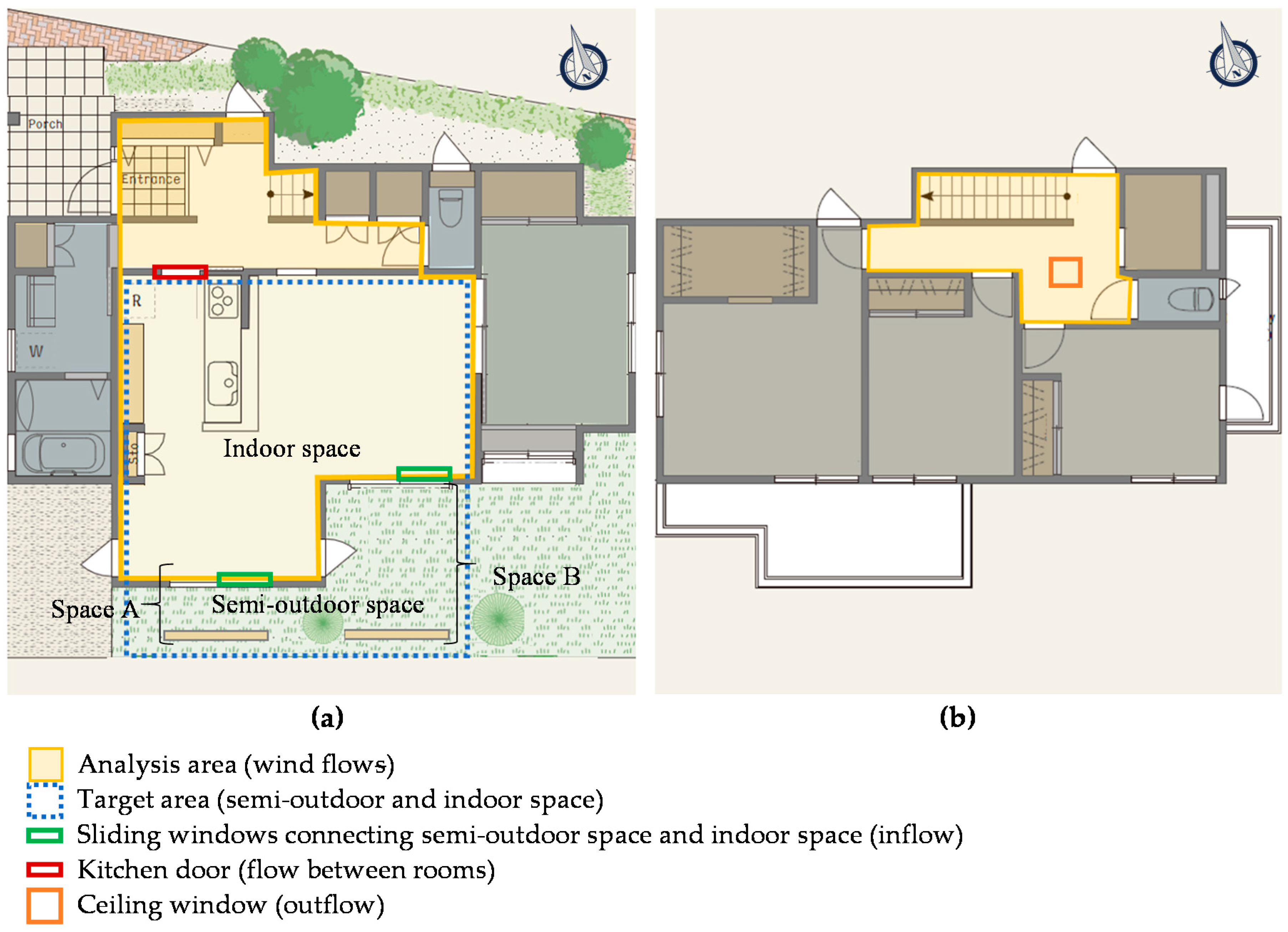
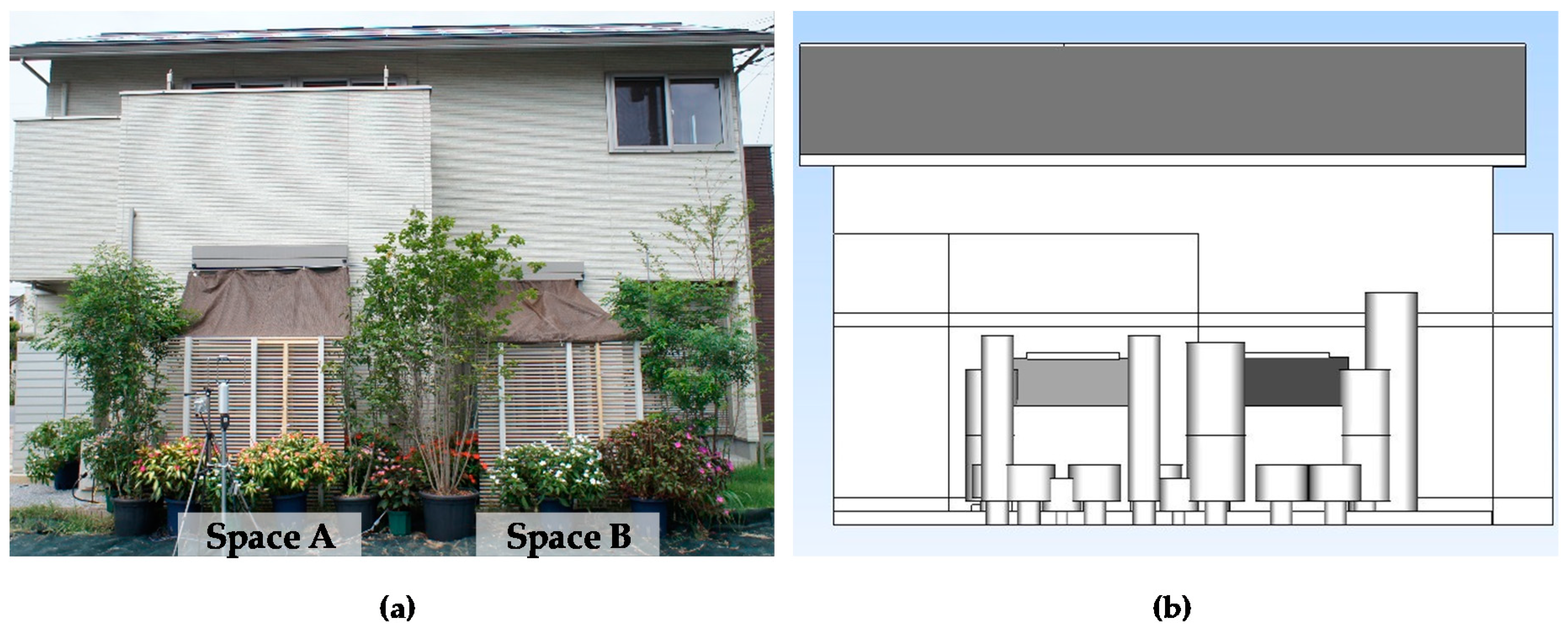
The field experiment was conducted in a two-story passive house located in a residential area (N36°8′50.6′′, E139°23′19.1′′) of Kumagaya City on September 12 and 17, 2016. This city has a humid subtropical climate (Cfa in the Köppen climate classification [52]) and one of the hottest summers in Japan [53]. The study was conducted during September (transition season), as the conditions were more appropriate for using evaporative cooling to extend the use of natural ventilation (after the hottest season). Recent weather data for the city (2007–2017) indicate that evaporative cooling has a cooling potential of 4.6–8.9 °C due to the water pressure deficit of air and wet surface during summer. To achieve the evaporative cooling effect, PCEs, comprised of an evaporative cooling louver [12], surrounding vegetation, and sunscreens attached from the top of the louver to the top of the window were installed in the outdoor space of the house. This space was connected to the common indoor space (kitchen, living room, and dining room) through two sliding windows, creating two semi-outdoor spaces: Spaces A and B, as shown in Figure 2 and Figure 3. The distance between the louver and window (L–W) for Space A was 1 m and for Space B was 2.8 m. The water supply during the experiment was 1.8 L/(m2h) for each evaporative cooling louver’s vertical plane. The supplied water temperature was 25 °C on average.
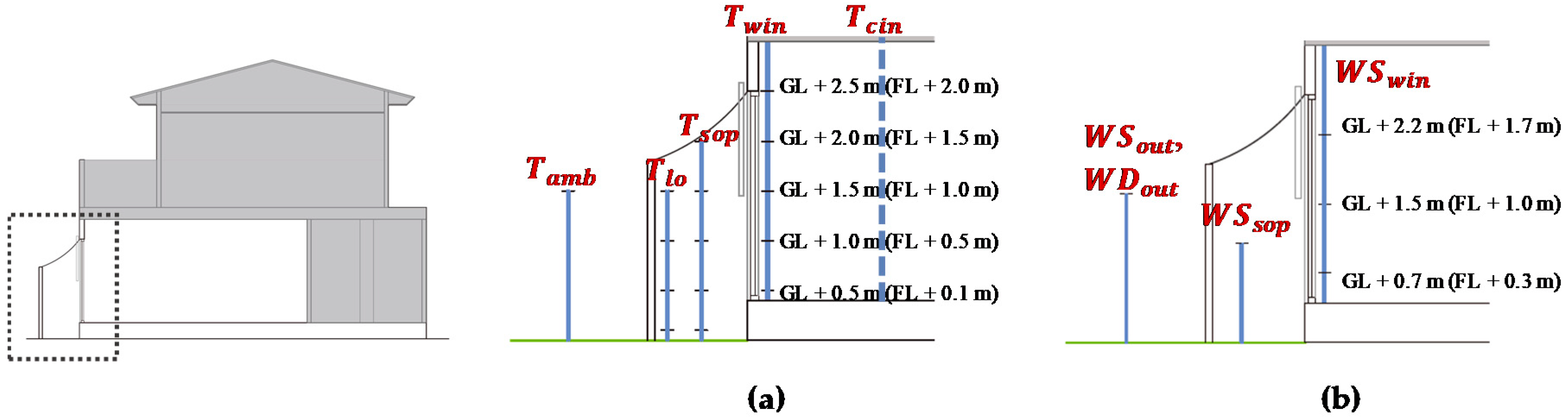
Measurement points for recording the vertical air temperature distribution were installed in the semi-outdoor space (back of the louver (Tlo)), center of the semi-outdoor space (Tsop), indoor space (inside the window (Twin)), and in the center of the indoor space (Tcin) at different heights above the ground (GL) (0.1–2.5 m) in Spaces A and B, as shown in Figure 4. In addition, ambient temperature (Tamb), solar radiation, and wind speed conditions, including outdoor wind speed and direction (WSout, WDout) and indoor wind speed and direction (WSwin, WDwin), were also recorded. Wind conditions in the semi-outdoor space were recorded only for Space A (WSsop, WDsop). The measurement equipment used and their accuracy are shown in Table 1.
The cooling effect of the PCEs was evaluated in a previous experimental study and cool air accumulation was confirmed mainly in Space A [14]. Among the several cases reported in the field measurements [14], the average data of one case (25 min) on September 12, 2016 were used to validate the CFD simulation in this study. This experimental case was selected as the PCEs and the ventilation settings with windows fully open were set to maximize the cooling effect with natural ventilation. Figure 2 shows the floor plan of the case study with the experimental settings of the selected case as follows: (1) the analysis area where air flows inside the house; (2) the openings for inflow (sliding windows), flow between rooms (kitchen door), and outflow (ceiling window); (3) the target area, comprised of the semi-outdoor spaces (Spaces A and B) and the indoor space. The air passing across the rooms and the kitchen door would flow out through the ceiling window located on the stair hall (Figure 2b). These conditions were used to validate the numerical simulation (Figure 3b).
3.3. CFD Simulations
A numerical CFD technique was selected to conduct the simulations. The commercial software scSTREAM (MSC software, Tokyo, Japan) was used to solve the steady Reynolds-averaged Navier–Stokes (RANS) equations to evaluate the average flow and temperature fields during the target evaluation time.
3.3.1. Computational Geometry, Domain, and Grid
Table 2 lists the calculation conditions used for the simulation. The size of the computational domain (calculation area) shown in Figure 5 was based on the best practice guidelines for CFD set by Franke et al. [54], Tominaga et al. [55], and Blocken [56]. This includes a distance of 5H from the building to the top and sides of the computational domain, and a distance of 15H between the building and the outlet boundary downstream of the building [57]. The resulting dimensions of the domain are shown in Table 2. To predict the flow field around a building with acceptable accuracy, a fine grid arrangement is required to resolve the flow near the corners, with a stretching ratio of the adjacent grid of 1.3 or less [55]. A relationship also exists between the size of the mesh and convergence. As the building model is complex and there are some materials with a large aspect ratio, a 100 mm mesh was used, as shown in Table 2. The computational domain was also discretized by a hexahedral mesh containing approximately 12 million elements, with an expansion ratio of 1.1.
3.3.2. Boundary Conditions
- Setting the inflow and outflow conditions.
Simulated isolated building conditions were comparable to those obtained by experiments at the site because when the field experiment was conducted, there was no building facing the semi-outdoor space and windward windows within a 20 m distance; thus, there was no obstruction of air flow. Therefore, in the CFD simulation, we set appropriate inflow boundary conditions to match the wind conditions measured in both spaces (i.e., WSout and WSwin) during the field experiment. As a result, a velocity of 1 m/s (maximum WSout recorded during the experiment) was set at a height of 1.5 m. Wind direction was set at 197° (SSW), the average of the maximum and minimum WDout recorded in the selected experimental case. The average recorded relative humidity was 56%. The standard k–ε model was used for turbulence, where the turbulent kinetic energy and dissipation were set to 0.173 m2/s2 and 0.0069 m2/s3, respectively. The remaining settings are listed in Table 2.
- Setting wall boundary conditions.
For the ground boundary, the log law condition was applied to the flow fields. For the top boundary of the computational domain, a symmetry boundary condition (slip wall) was used.
- Setting thermal boundary conditions.
The surface temperature (Ts) of the building elements was based on thermal imagery captured by an infrared camera (Thermo GEAR G100, Nippon Avionics Co., Ltd., Tokyo, Japan) during the experiment. The heat transfer coefficients used for the outdoor and indoor geometry were 11.6 and 9.5 W/m2k, respectively [58], including the effect of solar radiation.
3.3.3. Solver Settings
The three-dimensional (3D) steady RANS equations were solved with a standard k-model. Second-order upwind discretization schemes were used for the momentum and turbulence equations. The Quadratic Upstream Interpolation for Convective Kinematics (QUICK) scheme was used for convection terms. The convergence criterion for all variables was 1 × 10⁻⁵. We confirmed this criterion was sufficient for convergence in this study, based on the calculation time.
3.3.4. Detailed Modeling
- Modeling of vegetation.
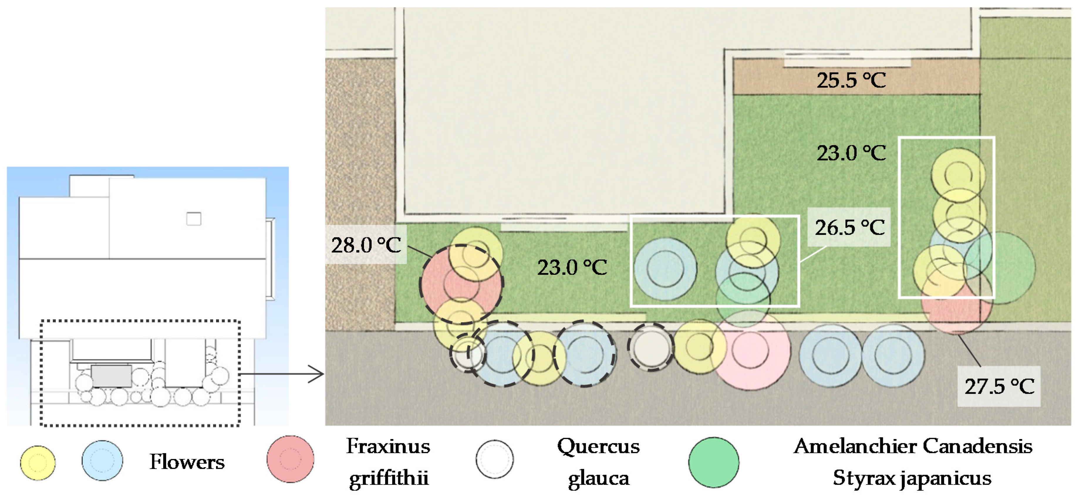
Vegetation consisted of plants (trees and flower pots) and ground covers in the semi-outdoor spaces. Plants were modeled with the same sizes and locations as the experiment using a cylindrical shape, as shown in Table 3 and Figure 6. The leaf area density (LAD) and drag coefficient (Cd) (Table 3) were estimated by observing the foliage density of each plant type using photos taken during the experiment. Accordingly, different LAD and Cd were assigned to each foliage density; these included high-density type 1 (HD1), high-density type 2 (HD2), low-density type 1 (LD1), high-density type 3 (HD3), and low-density type 2 (LD2). The values used for the LAD and Cd of plants were based on the resistance [59] and turbulence model B by Mochida (2008) [60] (see Table 4). For ground cover inside the semi-outdoor space (HD3 and LD2), as Ts was significantly lower than that of plants (refer to Figure 6), the LAD and Cd were estimated to achieve a higher cooling effect than the plants due to the watered soil. A previous study [61] showed that the average porosity for one, two and three trees was 0.91, 0.69, and 0.42, respectively. When porosity had reduced, more flow was forced around the plant. Moreover, the fitting equation of permeability in turbulent flow has greater accuracy when the vegetation porosity ranges from 0.9 to 1.0 [62]. For HD and LD types, porosities of 0.90 and 0.99, respectively, were assigned. The average surface temperature, shown in Figure 6, was derived from thermal imagery captured during the experiment. As observed, the Ts of the plants was 28.0 °C with direct solar radiation (dashed black), 27.5 °C when semi-shaded, and 26.5 °C when shaded (inside white square) during the evaluation time. The Ts of ground cover was 23.0 °C inside the semi-outdoor space and 25.5 °C near the window in Space B. A model constant of 1.8 was selected because it can accurately reproduce the velocity deficit effect downwind of the trees and has been shown produce good correspondence between calculations and measurements [60]. The convective heat transfer coefficient (CHTC) of plants was based on Asawa et al. [63] and was estimated by the following equation:
where [m/s] is the inflow fixed velocity for the entire crown. The CHTC were double the value given by the Jürges relation formula [63]. The CHTC of ground cover were derived from Hagishima et al. [64] and are shown in Table 3. A constant moisture flux of 0.1 g/m2s was set for vegetation with high foliage density; this applied to HD1, HD2, and HD3.
- Modeling of porous media: evaporative cooling louver and window net.
The evaporative cooling louver has a complex geometry with an acute angle toward the windward direction, considered to result in less drag with a higher evaporative cooling effect [12]. To save calculation load and time with appropriate drag and cooling effects, the evaporative cooling louver was modeled as a porous media anisotropic model containing a solid and fluid as an alternative to generating fine mesh elements. Figure 7 shows that the length and height of the louver was 1.8 m, and louver thickness was set to 0.1 m to match mesh size. Similarly, the window net was modeled as porous media, with length and height based on one panel of the sliding window (0.70×2.10 m), and a thickness of 0.1 m. Table 5 presents the inputs of the porous media (louver and window net), which include the CHTC, surface area ratio (surface area/volume mesh), porosity (volume ratio/volume mesh), fixed temperature, cross-sectional area ratio (area/area mesh), and pressure loss. For the CHTC of the louver, the heat transfer model of the louver developed by Hirayama et al. [65] was employed. The CHTC [W/m2k] of the louver was based on the following equation:
where is the inflow fixed velocity [m/s].
As presented in Table 5, a fixed surface temperature of 23.5 °C (watered) was assigned to the louver, and no heat generation was assigned to the window net to avoid affecting the surrounding air temperature. For surface area ratio, porosity, and cross-sectional area ratio, the data of one mesh were inputted, as shown in Figure 7. Therefore, the front view (Y axis) and side view (X axis) of one mesh was used to calculate the surface area, volume ratio, and cross-sectional area ratio. For the louver, the surface area used to calculate the ratio was obtained by multiplying the circumference of one slat (0.153 m) by the number of slats in one mesh (2.5 slats) and the thickness of the mesh (0.1 m). The volume ratio of one mesh used to calculate porosity was obtained by multiplying the volume of one slat by the number of slats in one mesh and the thickness of one mesh. Similarly, the same data were calculated for the window net by assuming an area of one hole of the net of 1.2 mm2 and a wire thickness of 0.2 mm. These results are summarized in Table 5. The pressure loss variations of the louver and window net are shown in Table 6. The pressure loss of the louver was obtained from the analysis model of Hirayama et al. [65], and the window net was estimated from the model in Minoru et al. [66], which used a similar net size (i.e., net4). A moisture of 1.177 g/s was set for the louver based on the evaporation rate of the louver [12] at the time of the field experiment. The porous media use the following equations for momentum (3), energy for fluid media (4) and solid media (5):
Momentum equation for porous media:
Energy equation for fluid media:
Energy equation for solid media:
where is the mean velocity in the i direction [m/s]; is the mean velocity for the j direction [m/s]; is the stress tensor [Pa]; is the gravitational acceleration in the i direction [m/s2]; is the pressure loss in the i direction per unit length [Pa/m] is the porosity of porous media [-] is the fluid density [kg/m3] is the solid density [kg/m3]; is the specific heat of fluid at constant pressure [J/(kg K)] is the specific heat of solid [J/(kg K)] is the heat conductivity of fluid [W/m] is the heat conductivity of solid [W/m]; is the fluid temperature [K]; is the solid temperature [K] is the heat generation in fluid per unit volume [W/m3] is the heat generation in solid per unit volume [W/m3] is the tensor of area ratio [-]; is the surface area ratio (contact ratio between the fluid and solid per unit volume) [m2/m3]; is the convective heat transfer coefficient [W/(m2 K)].
3.4. Simulation Cases
Table 7 shows the simulation cases for all conditions used for validation and sensitivity analysis. To ensure controlled conditions, only one variable was changed at a time. As previously mentioned, this study mainly focused on replicating and analyzing the formation of cool air in a semi-outdoor space. Thus, the settings in the semi-outdoor space were altered, whereas the settings in the indoor space were kept constant. For the validation case S-0, the settings in the semi-outdoor space reproduce the field experiment case. As such, case S-0 was used as the base case for sensitivity analysis to analyze the cooling effects of the PCEs under various conditions, including louver watering conditions and the number of PCEs. The effect of louver watering conditions is represented by cases S-0–S-2. The effect of the number of PCEs on the formation of cool air is represented by cases S-3–S-5. Only the sunscreen remained installed in the semi-outdoor space to maintain the initial thermal boundary conditions for the building elements and ground cover. To simulate different watering louver conditions, the louver Ts was modified. For the watered louver condition, based on previous research [14], the Ts of the watered louver was approximately 4 °C lower than Tamb; thus, 23.5 °C was applied. Moreover, when the louver was wet, Ts was approximately 2 °C lower than Tamb; 25.5 °C was applied. For the dry louver, Ts was set to 29 °C as the solar radiation during the experiment was relatively low.
4. Results
4.1. Validation
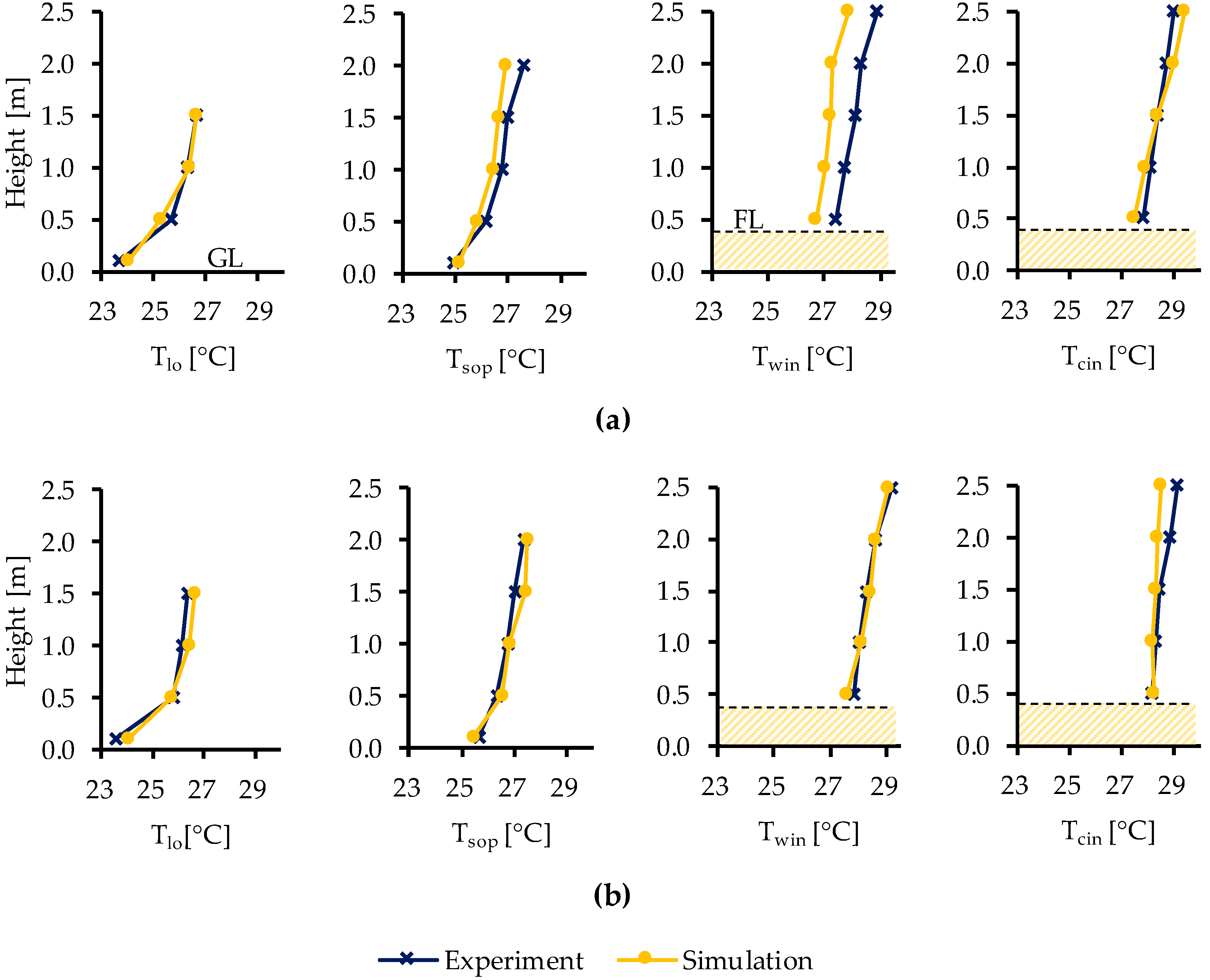
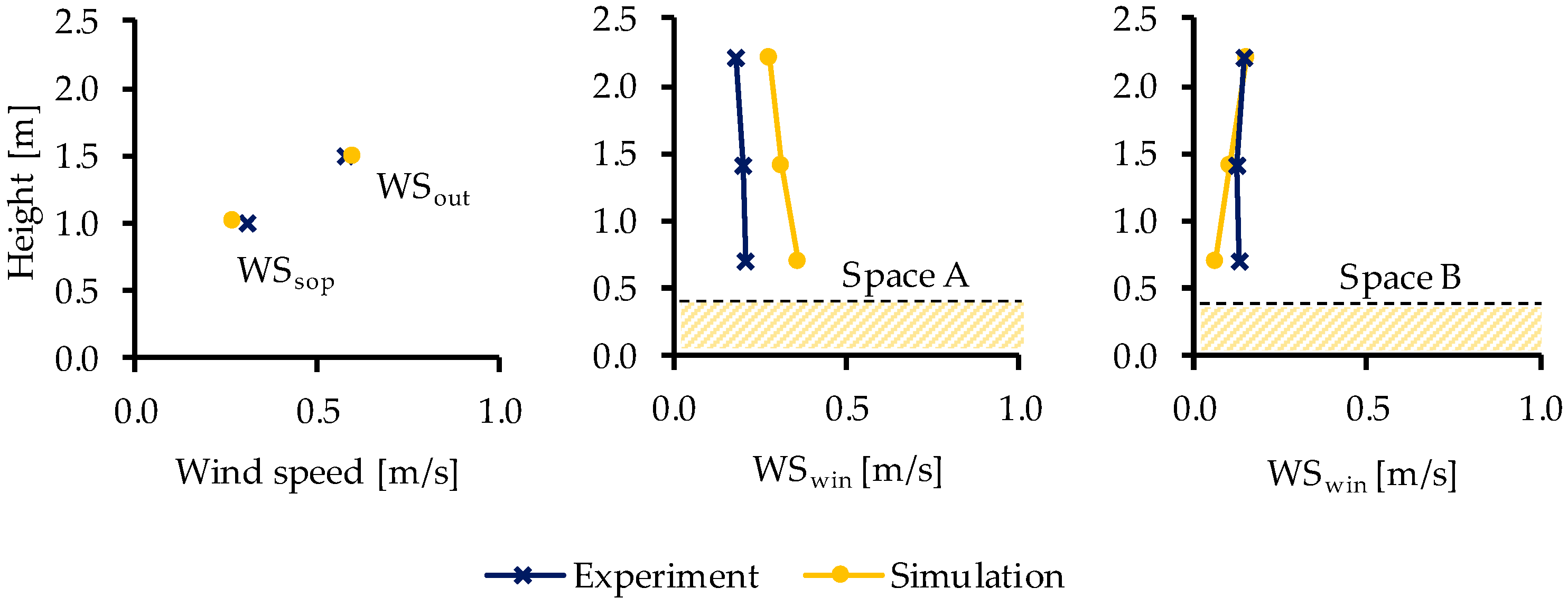
Figure 8 presents the vertical temperature distribution for each measurement point for the semi-outdoor and indoor spaces between the experiment and simulation (case S-0). Table 8 shows the correlation and deviation between the experiment and simulation at each measurement point. Figure 9 compares the wind speed for the outdoor, semi-outdoor, and indoor spaces between the experiment and simulation. According to the vertical temperature distribution in Figure 8, cool air formation occurs near the ground in the semi-outdoor spaces (Spaces A and B) in the experiment and simulation, indicating that the cooling effects of the PCEs were replicated in the simulation. In general, the results for Spaces A and B show good correlation between the experiment and simulation (Table 8). The coefficient of determination (R2) for all points was between 0.93 and 0.99, and the root mean square error (RMSE) was between 0.2 and 0.5 except for Twin, demonstrating that the model accurately predicts the data. However, for the point Twin at Space A, the RMSE was close to 0.9. This is because the model overpredicts the wind speed through the window (WSwin). The WSwin was approximately 0.2 m/s (Figure 9), higher than that recorded during the experiment. It was assumed that this causes Twin to be slightly cooler, as more cool air flows through the window, resulting in a maximum air temperature difference of 0.7–1.0 °C for GL+0.5 m to GL+2.5 m (Figure 8a). Despite this, good correlation was observed for Tcin (air temperature in the center of the indoor space/representative indoor air temperature) in Spaces A and B, indicating that the model accurately predicts indoor air temperature. Overall, the vertical air temperature distribution showed a consistent trend between the experiment and simulation, demonstrating that the model can effectively predict conditions observed during the experiment.
4.2. Sensitivity Analysis
4.2.1. Watering Conditions of the Evaporative Cooling Louver
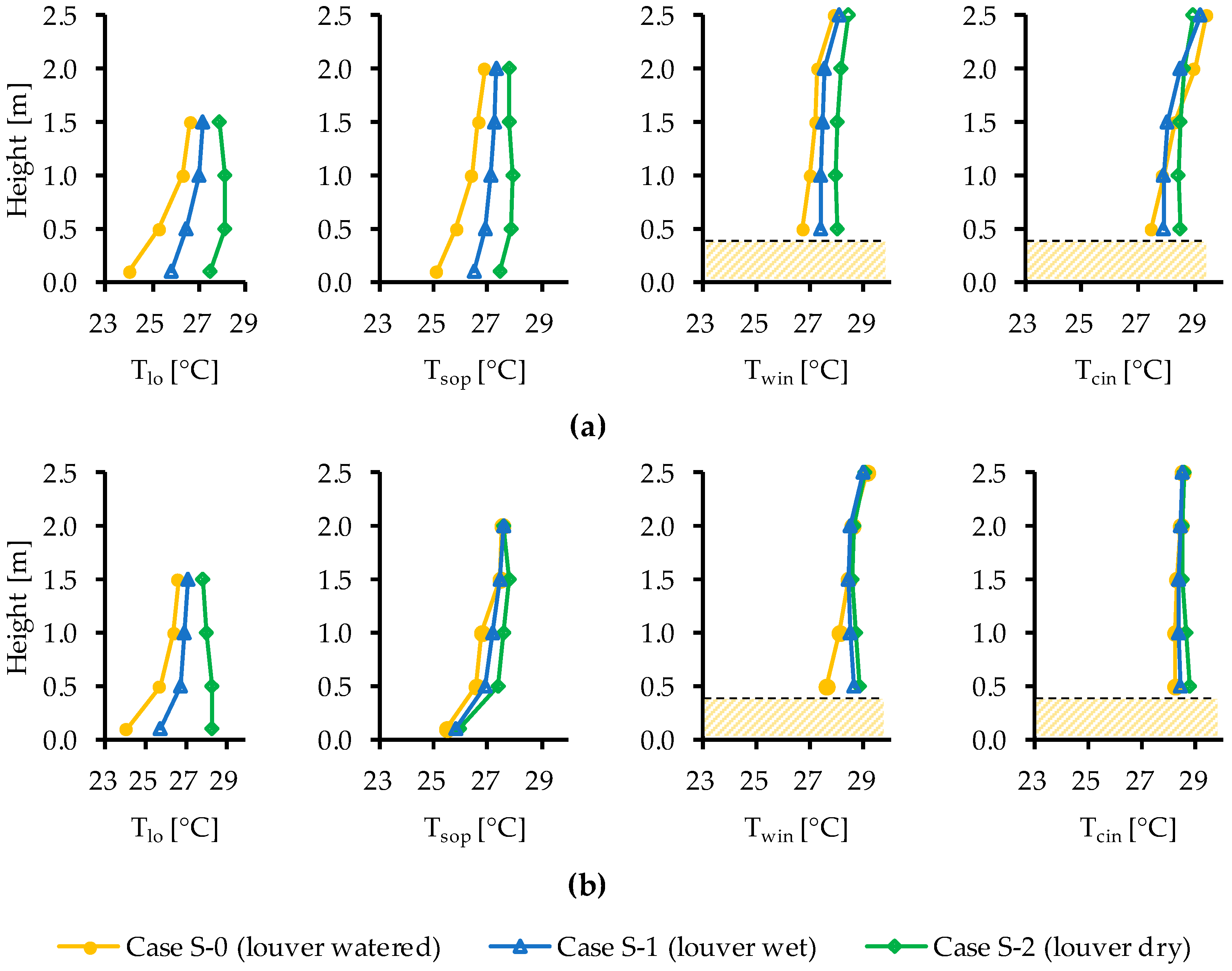
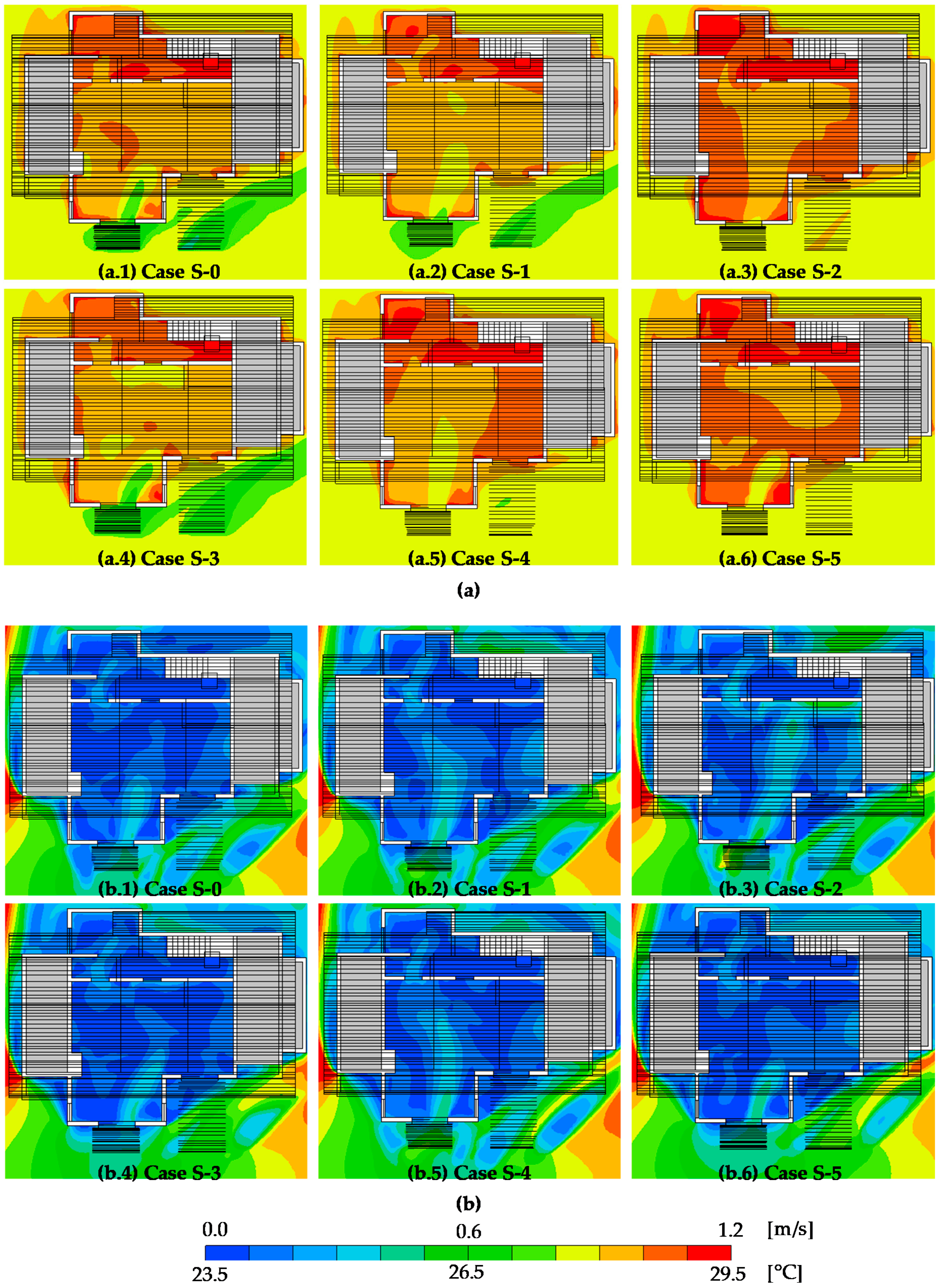
Figure 10 shows the sensitivity analysis results for the formation of cool air in the semi-outdoor space and the subsequent cooling effect in the indoor space for different louver watering conditions. Figure 11 shows the air temperature and wind speed contours for each case at the measurement point GL+1.5 m, that is, 1.5 m above the outdoor ground or 1.0 m above the indoor floor level. Figure 12 shows the air temperature and wind speed contours at GL+1.5 m for each simulated case. In Figure 10, the results show that when the louver watering condition is applied and its Ts is close to the wet-bulb temperature, the validation case S-0 can effectively predict the formation of cool air in the semi-outdoor space compared to other cases. Moreover, the results for cases S-1 and S-2 show that when the watering stops and the Ts of the louver is increased, the evaporative cooling effect of the louver, shown in Tlo, significantly reduces. In case S-1, when the louver is wet, the cooling effect of Tlo from GL+0.1 m to GL+1.5 m is reduced by approximately 1.8–0.6 °C for Space A, and 1.7–0.5 °C for Space B, compared to the initial case S-0. Moreover, when the louver is dry in case S-2, the cooling effect at Tlo from GL+0.1 m to GL+1.5 m is further reduced by approximately 3.4–1.3 °C for Space A and 4.3–1.2 °C m for Space B. For Tsop (measurement point at the center of the semi-outdoor space), the reduction in cooling effect differed greatly between Spaces A and B because of the louver–window (L–W) distance. The L–W distance was 1 m for Space A and 2.8 m for Space B. Thus, for Space A in case S-1, the cooling effect at Tsop had reduced by approximately 1.3–0.4 °C from GL+0.1 m to GL+2.0 m. In contrast, for Space B in case S-1, the cooling effect at Tsop had only reduced by approximately 0.35–0.1 °C from GL+0.1 m to GL+2.0 m. This demonstrates that the cooling effect reduces with increasing distance from the evaporative cooling louver. This means shorter L–W distance is preferable when the evaporative cooling louver is used to form cool air in a semi-outdoor space. This is confirmed when observing the air temperature contours at GL+1.5 m in Figure 12a.1,a.2, where the formation and cooling effect (watered and wet louver) is better for Space A than Space B. In Space B, the combination of factors such as the L–W distance, amount of vegetation, and wind direction (Figure 12b.1,b.2), directly affects the accumulation of cool air in the semi-outdoor space and the cool air does not reach the window–indoor space. With a larger L–W distance, the generation of cool air in the semi-outdoor space and the flow of cool air into the indoor space is more difficult than with a shorter L–W distance in Space A. Based on Figure 10, for case S-2, the cooling effect of Tsop from GL+0.1 m to GL+2.0 m had reduced by 2.3–0.9 °C for Space A and 0.5–0.4 °C for Space B. When the louver was dry (case S-2), there was no cool air produced in the semi-outdoor space (Figure 12a.3); thus, Tlo and Tsop at point GL+1.5 m are similar to the ambient temperature. Furthermore, Figure 10 (point Tcin) and Figure 12a.1,a.4 show that the cool air accumulated in semi-outdoor Space A could not effectively cool the entire indoor space with the current indoor variables (window-opening conditions, indoor door opening, and leeward openings; see Figure 2). This is clearly seen by comparing cases S-0, S-1, and S-2, where no significant difference was observed in Tcin. Despite there being a difference for Twin in Space A, in reality, this point could be properly reproduced, as described in the previous section. Thus, only points Tlo, Tsop, and Tcin were appropriate for a comparative analysis.
4.2.2. Amount of Passive Cooling Material in the Semi-Outdoor Space
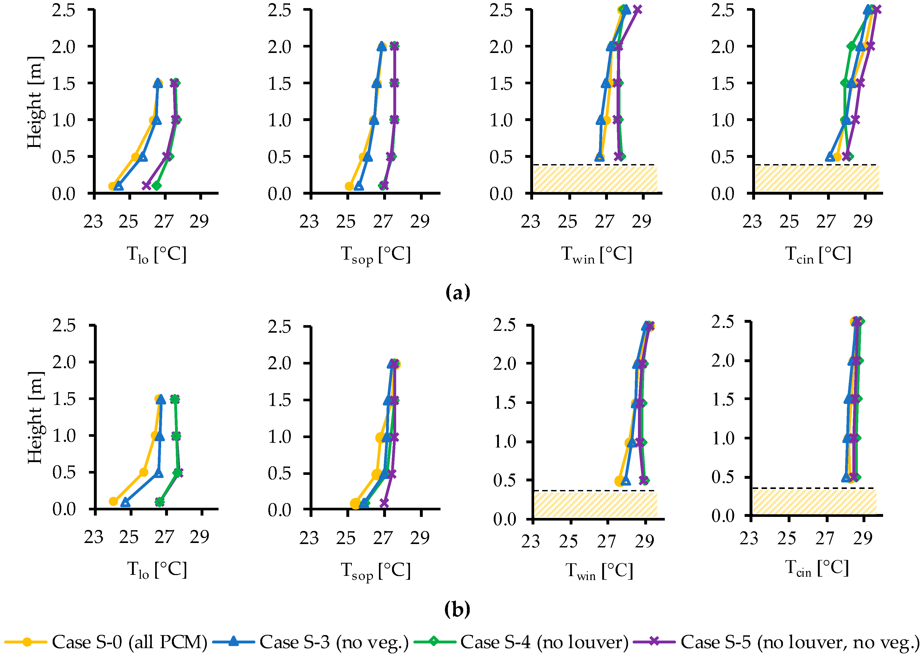
This section analyzes the individual effect of each PCE. As shown in Table 7, all PCEs were applied to case S-0; case S-3 had no vegetation, case S-4 had no louver, and case S-5 had no louver and no vegetation. The vertical air temperature distribution in these cases is presented in Figure 11. For cases S-0 and S-3, the shorter L–W distance in Space A and use of the evaporative cooling louver resulted in a higher cooling effect (Tlo) and better formation of cool air (Tsop). When the vegetation was removed in case S-3, the air temperature at Tlo in Space A only increased by approximately 0.3–0.1 °C for GL+0.1 m to GL+1.0 m. This is in contrast to when the louver was removed in cases S-4 and S-5, where air temperature at Tlo increased by 2.5–1.0 °C and 1.9–0.9 °C for GL+0.1 m to GL+1.5 m, respectively. In contrast, for Space B, the lack of vegetation in case S-3 resulted in a further increase at Tlo of approximately 0.7–0.1 °C for GL+0.1 m to GL+1.5 m; twice the cooling effect lost in Space A at all points. This suggests that the use of surrounding vegetation is more beneficial for obtaining a higher cooling effect and generating more cool air at a larger L–W distance than at a shorter L–W distance in Space A. This is more explicitly shown in Space B for cases S-4 and S-5, where air temperature at case S-4 (only vegetation) Tsop increases by 0.5–0.1 °C for GL+0.1 m to GL+1.5 m, in contrast to case S-5, where air temperature in Tsop increases by 1.5–0.1 °C.
4.2.3. Cooling the indoor space
For cases with wet and watered louvers, the generation and flow of cool air is evident in Space A (Figure 12a.1,a.2,a.4). In contrast, the cool air formed by the louver does not reach the window in Space B, mostly due to the large L–W distance and wind; this clearly contributes to the dissipation of cool air through the side. Regarding the presence of vegetation, a comparison of cases S-3 (Figure 12a.4) and S-0 (Figure 12a.1) shows that the cool air generated in the semi-outdoor space easily dissipates when vegetation was removed in Spaces A and B. A comparison of cases S-0 and S-3 (in Figure 12a.1,a.4,b.1,b.4) shows that the wind speed through the window was higher in the latter case due to the lack of vegetation, allowing more cool air to flow through the window and further cooling the indoor space. Thus, although vegetation enhances the cooling effect near the louver, it may prevent cool air from dissipating into the indoor space. This suggests that vegetation is not necessary for a shorter L–W distance. For cases S-0 and S-4 (Figure 12a.1,a.5,b.1,b.5), vegetation had different effects on wind speed and flow of air because the combination of the vegetation and the louver significantly reduced the wind speed in case S-0. This was unlike case S-4 without the louver, where only vegetation resulted in a higher wind speed through the window. Generally, the use of solar shading (sunscreen) alone (case S-5) results in the worst-case scenario.
As seen in the indoor space, a better cooling effect was observed when using the watered louver (cases S-0 and S-3). In addition, a comparison between Spaces A and B shows that a shorter L–W distance is more beneficial for cooling the indoor space than a longer L–W distance, where controlling the wind direction and inducing cool air is more difficult. The results for all cases demonstrate that the ventilation strategies employed during the experiment (Figure 2) restrict indoor flow due to a lack of leeward openings; this meant the effective induction of cool air was restricted. In general, the results show that the louver is effective for indoor cooling if a combination of proper installation (shorter L–W distance) and indoor ventilation strategies are applied.
5. Discussion
The validation results of the CFD simulation with detailed modeling of PCEs show that this model can effectively predict the cooling effect of PCEs for a semi-outdoor space. The maximum difference in air temperature between the experiment and simulation was obtained at Twin (0.7–1 °C) in Space A. This difference was considered acceptable for CFD simulations, considering the model simplification and assumptions (i.e., average steady-state flow calculations in the CFD, limited boundary conditions, imperfect agreement with experimental conditions), and considering the following points. Previous studies that compared experimental and simulated air temperatures in outdoor spaces with cool materials and vegetations reported a mean absolute error of 1.34 °C on average, 3.67 °C as a maximum, and 0.27 °C as a minimum [23]. The reported R2 was 0.92 on average, 0.99 as a maximum, and 0.66 as a minimum. In our study, the R2 was between 0.93 and 0.99 for all measurement points. Therefore, our results show better accuracy than those previously reported in the literature. In terms of human thermal comfort for passive cooling, the sensitivity of human skin to temperature differences is approximately 1 °C [67]. Regarding the temperature experiments in the outdoor spaces used for validation, measurement errors of approximately 0.7 °C are inevitable [4]. Therefore, the simulation and modeling are considered to have appropriate accuracy for discussing the cooling effects of PCEs.
For sensitivity analysis, a similar reduction in temperature was observed between the louver watering conditions of cases S-0 (watered louver) and S-2 (dry louver) in Space A in a previous study [14]. Here, the Tlo had reduced by approximately 2.8–1.2 °C from GL+0.1 m to GL+1.5 m after the louver was watered, and had reduced by 3.4–1.3 °C in the simulation. This confirms that the cooling effect of the louver watering conditions was successfully reproduced with this model.
In terms of the effect of the L–W distance, Del Rio et al. (2019) [14] indicated that cool air generated by the louver in Space B could potentially dissipate through the side prior to reaching the window. The simulation results in Figure 12 support this hypothesis as the wind speed contours in Figure 12 show that air passing through the louver with relatively high wind speed did not flow toward the window and instead, flowed toward the corner of the wall. Therefore, to obtain a higher cooling effect (cool breeze) in the indoor space, the louver should be installed close to the window and kept watered, and vegetation should not be used (i.e., case S-3 in Space A). The louver and vegetation also showed more positive effects when implemented alone than in combination. In general, the results indicate that the evaporative cooling louver has a higher cooling effect than vegetation. In addition, the Twin and WSwin results (case S-0) reveal that cool air was induced indoors when the wind speed through the window was greater than 0.2 m/s, similar to the conclusions of a previous study [14].
This study conducted validation and sensitivity analysis of CFD simulations related to the formation of cool air in semi-outdoor spaces using PCEs. Although the indoor space variables were not investigated in detail, the validated model was able to replicate the representative indoor air temperature (Tcin), and therefore, the effect of ventilation parameters employed in the field experiment (Figure 2). This suggests that future studies investigating the indoor space variables such as window type, porosity of the building, size of indoor space, and location of furniture, would provide useful insights for the design of cross ventilation between openings and indoor spaces to optimize the flow of cool air indoors. Greater cooling was obtained in the semi-outdoor space by using the evaporative cooling louver and a sunscreen. This combination has the potential to reduce indoor temperatures with appropriate ventilation. Future research should investigate these variables to determine the most optimal method to enhance the natural ventilation potential of a residence, transferring cool air indoors from semi-outdoor spaces.
6. Conclusions
This study demonstrates a modeling method and presents validated results for cool microclimates using PCEs in the semi-outdoor space of a passive house located in one of Japan’s hottest cities. The PCEs used consisted of an evaporative cooling louver [12], surrounding vegetation, and a sunscreen. The results showed good correlation between the experiment and simulation for Spaces A and B. The R2 for all points was between 0.93 and 0.99, and the RMSE was between 0.2 and 0.5 except for the window position (Twin), demonstrating that the model accurately predicts the air temperature. The maximum temperature difference was observed at Twin; however, the difference was within 1 °C. These results show that the modeling method and parameters applied in the CFD simulation were able to reproduce the vertical air temperature distributions in semi-outdoor and indoor spaces observed during a previous field experiment [14].
A sensitivity analysis was conducted for the variables in the semi-outdoor spaces, and the individual and combined effects of the PCEs were confirmed. The louver model with porous media was able to reproduce the cooling effect between different louver watering conditions (watered, wet, and dry). Similar air temperature reductions were obtained between dry and watered louver conditions in the simulation and experiment (approximately 1–3 °C). In addition, the effect of different louver–window (L–W) distances on the generation of cool air in the semi-outdoor space was similar between the simulation and experiment. A shorter L–W distance was found to be the most effective, as the louver was closer to the window, enabling cool air to be more easily generated by the watered louver. At a greater L–W distance, cool air dissipated through the sides prior to reaching the window. The sensitivity analysis also showed that vegetation was not necessary with a shorter L–W distance.
This study confirms that the evaporative cooling louver can generate cool microclimates inside buildings under certain conditions, i.e., when it is watered; placed near the target area; faces a predominant wind direction; used in daytime when relative humidity is about 50–70%; during transition seasons (after hottest season), to aid mixed mode ventilation. In addition, to cool the indoor space with adequate natural ventilation, techniques such as cross and/or stack ventilation avoiding single sided ventilation are applied. Moreover, this study demonstrated that CFD simulations with the detailed PCE parameters can be effectively used to evaluate the cooling effects of PCEs on the microclimate. As the main focus of this study was on the semi-outdoor space, indoor variables should be studied in the future to determine better ventilation strategies for improving the flow of cool air into indoor spaces. In addition, an evaluation of residents’ thermal comfort is also necessary. This study encourages the implementation of passive cooling methods in microclimate design to help mitigate uncomfortable urban thermal environments and ensure the health and quality of life for present and future generations.
Author Contributions
Conceptualization, M.A.D.R., T.A., and Y.H.; Data curation, M.A.D.R.; Formal analysis, M.A.D.R.; Investigation, M.A.D.R., Y.H.; Methodology, M.A.D.R., T.A., and Y.H.; Project administration, T.A.; Resources, T.A.; Supervision, T.A.; Validation, M.A.D.R.; Visualization, M.A.D.R.; Writing—original draft, M.A.D.R.; Writing—review and editing, M.A.D.R., T.A., and Y.H. All authors have read and agreed to the published version of the manuscript.
Funding
This research received no external funding.
Conflicts of Interest
The authors declare no conflict of interest.
Nomenclature
| Ambient temperature [°C] | |
| Outdoor wind speed [m/s] | |
| Outdoor wind direction [°] | |
| Air temperature at the back of the louver [°C] | |
| Air temperature at the center of the semi-outdoor space [°C] | |
| Wind speed at the semi-outdoor space [m/s] | |
| Air temperature inside the window [°C] | |
| Air temperature at the center of the indoor space [°C] | |
| Wind speed inside the window [m/s] | |
| Surface temperature [°C] | |
| Inflow fixed velocity [m/s] | |
| Extra term added in the momentum equation | |
| Extra term added in the transport equation of | |
| Extra term added in the transport equation of | |
| Fraction of the area covered with plants | |
| Leaf area density (LAD) | |
| Drag coefficient | |
| Turbulence energy | |
| Energy dissipation rate | |
| Model constant | |
| Mean velocity for i direction [m/s] | |
| Mean velocity for j direction [m/s] | |
| Stress tensor [Pa] | |
| Gravitational acceleration for i direction [m/s2] | |
| Pressure loss for i direction per unit length [Pa/m] | |
| Porosity of porous media [-] | |
| Fluid density [kg/m3] | |
| Solid density [kg/m3] | |
| Specific heat of fluid at constant pressure [J/(kg K)] | |
| Specific heat of solid [J/(kg K)] | |
| Heat conductivity of fluid [W/m] | |
| Heat conductivity of solid [W/m] | |
| Fluid temperature [K] | |
| Solid temperature [K] | |
| Heat generation in fluid per unit volume [W/m3] | |
| Heat generation in solid per unit volume [W/m3] | |
| Tensor of area ratio [-] | |
| Surface area ratio (contact ratio between fluid and solid per unit volume) [m2/m3] | |
| Convective heat transfer coefficient [W/(m2 K)] |
References
- Iyendo, T.O.; Akingbaso, E.Y.; Alibaba, H.Z.; Özdeniz, M.B. A relative study of microclimate responsive design approaches to buildings in cypriot settlements. A/Z ITU J. Fac. Arch. 2016, 13, 69–81. [Google Scholar] [CrossRef]
- Drach, P.R.C.; Karam-Filho, J. Increasing ventilation by passive strategies: Analysis of indoor air circulation changes through the utilization of microclimate elements. Appl. Math. 2014, 5, 442–452. [Google Scholar] [CrossRef] [Green Version]
- Yi, C.Y.; Peng, C. Microclimate Change outdoor and indoor coupled simulation for passive building adaptation design. Procedia Comput. Sci. 2014, 32, 691–698. [Google Scholar] [CrossRef] [Green Version]
- Lee, T.C.; Asawa, T.; Kawai, H.; Sato, R.; Hirayama, Y.; Ohta, I. Multipoint measurement method for air temperature in outdoor spaces and application to microclimate and passive cooling studies for a house. Build. Env. 2017, 114, 267–280. [Google Scholar] [CrossRef]
- Elwy, I.; Ibrahim, Y.; Fahmy, M.; Mahdy, M. Outdoor microclimatic validation for hybrid simulation workflow in hot arid climates against ENVI-Met and field measurements. Energy Procedia 2018, 153, 29–34. [Google Scholar] [CrossRef]
- McGrane, S.J. Impacts of urbanisation on hydrological and water quality dynamics, and urban water management: A review. Hydrol. Sci. J. 2016, 61, 2295–2311. [Google Scholar] [CrossRef]
- Zhang, B.; Gao, J.; Yang, Y. The cooling effect of urban green spaces as a contribution to energy-saving and emission-reduction: A case study in Beijing, China. Build. Env. 2014, 76, 37–43. [Google Scholar] [CrossRef]
- Toparlar, Y.; Blocken, B.; Vos, P.; Van Heijst, G.J.F.; Janssen, W.D.; van Hooff, T.; Montazeri, H.; Timmermans, H.J.P. CFD simulation and validation of urban microclimate: A case study for Bergpolder Zuid, Rotterdam. Build. Env. 2015, 83, 79–90. [Google Scholar] [CrossRef] [Green Version]
- Santamouris, M.; Asimakopoulos, D. Passive Cooling of Buildings; James & James, Science Publishers Ltd.: London, UK, 1996. [Google Scholar] [CrossRef]
- Santamouris, M.; Kolokotsa, D. Passive cooling dissipation techniques for buildings and other structures: The state of the art. Energy Build. 2013, 57, 74–94. [Google Scholar] [CrossRef]
- He, J.; Hoyano, A. Experimental study of practical applications of a passive evaporative cooling wall with high water soaking-up ability. Build. Env. 2011, 46, 98–108. [Google Scholar] [CrossRef]
- Hirayama, Y.; Ohta, M.I.; Hoyano, A.; Asawa, T. Thermal performance of a passive cooling louver system to form cool microclimate in urban residential outdoor spaces. In Proceedings of the 30th International PLEA Conference, CEPT University, Ahmedabad, Inida, 16–18 December 2014. [Google Scholar]
- Hirayama, Y.; Asawa, T.; Sato, R.; Ohta, I.; Sumi, N. Study on design method for cool spot formation in a semi-outdoor space by combining various passive cooling techniques. J. Env. Eng. 2018, 83, 193–203. [Google Scholar] [CrossRef] [Green Version]
- Del Rio, M.A.; Asawa, T.; Hirayama, Y.; Sato, R.; Ohta, I. Evaluation of passive cooling methods to improve microclimate for natural ventilation of a house during summer. Build. Env. 2019, 149, 275–287. [Google Scholar] [CrossRef]
- Maerefat, M.; Haghighi, A.P. Natural cooling of stand-alone houses using solar chimney and evaporative cooling cavity. Renew. Energy 2010, 35, 2040–2052. [Google Scholar] [CrossRef]
- Wong, N.H.; Chong, A.Z.M. Performance evaluation of misting fans in hot and humid climate. Build. Env. 2010, 45, 2666–2678. [Google Scholar] [CrossRef]
- Urano, Y.; Watanabe, T.; Hayashi, T.; Uchiyama, A. Study on thermal environment of traditional vernacular houses in Northern Kyushu. J. Arch. Plan. Env. Eng. AIJ 1987, 371, 27–37. [Google Scholar] [CrossRef] [Green Version]
- Toparlar, Y.; Blocken, B.; Maiheu, B.; van Heijst, G.J.F. A review on the CFD analysis of urban microclimate. Renew. Sustain. Energy Rev. 2017, 80, 1613–1640. [Google Scholar] [CrossRef]
- Crank, P.J.; Sailor, D.J.; Ban-Weiss, G.; Taleghani, M. Evaluating the ENVI-met microscale model for suitability in analysis of targeted urban heat mitigation strategies. Urban Clim. 2018, 26, 188–197. [Google Scholar] [CrossRef]
- Forouzandeh, A. Numerical modeling validation for the microclimate thermal condition of semi-closed courtyard spaces between buildings. Sustain. Cities Soc. 2018, 36, 327–345. [Google Scholar] [CrossRef]
- Égerházi, L.A.; Kovács, A.; Unger, J. Application of microclimate modelling and onsite survey in planning practice related to an urban micro-environment. Adv. Meteorol. 2013, 2013. [Google Scholar] [CrossRef]
- Liu, Z.; Zheng, S.; Zhao, L. Evaluation of the ENVI-met Vegetation model of four common tree species in a subtropical hot-humid area. Atmosphere 2018, 9, 198. [Google Scholar] [CrossRef] [Green Version]
- Tsoka, S.; Tsikaloudaki, A.; Theodosiou, T. Analyzing the ENVI-met microclimate model’s performance and assessing cool materials and urban vegetation applications—A review. Sustain. Cities Soc. 2018, 43, 55–76. [Google Scholar] [CrossRef]
- Chatzinikolaou, E.; Chalkias, C.; Dimopoulou, E. Urban microclimate improvement using ENVI-met climate model. Int. Arch. Photogramm. Remote Sens. Spat. Inf. Sci. 2018, XLII-4, 69–76. [Google Scholar] [CrossRef] [Green Version]
- Baglivo, C.; Congedo, P.M. Design method of high performance precast external walls for warm climate by multi-objective optimization analysis. Energy 2015, 90, 1645–1661. [Google Scholar] [CrossRef]
- Congedo, P.M.; Baglivo, C.; Centonze, G. Walls comparative evaluation for the thermal performance improvement of low-rise residential buildings in warm mediterranean climate. J. Build. Eng. 2020, 28, 101059. [Google Scholar] [CrossRef]
- Saffari, M.; de Gracia, A.; Ushak, S.; Cabeza, L.F. Passive cooling of buildings with phase change materials using whole-building energy simulation tools: A review. Renew. Sustain. Energy Rev. 2017, 80, 1239–1255. [Google Scholar] [CrossRef] [Green Version]
- Bhamare, D.K.; Rathod, M.K.; Banerjee, J. Passive cooling techniques for building and their applicability in different climatic zones—The state of art. Energy Build. 2019, 198, 467–490. [Google Scholar] [CrossRef]
- He, J.; Hoyano, A.; Asawa, T. A Numerical simulation tool for predicting the impact of outdoor thermal environment on building energy performance. Appl. Energy 2009, 86, 1596–1605. [Google Scholar] [CrossRef]
- Allegrini, J.; Dorer, V.; Carmeliet, J. Impact of radiation exchange between buildings in urban street canyons on space cooling demands of buildings. Energy Build. 2016, 127, 1074–1084. [Google Scholar] [CrossRef]
- de La Flor, F.S.; Dominguez, S.A. Modelling microclimate in urban environments and assessing its influence on the performance of surrounding buildings. Energy Build. 2004, 36, 403–413. [Google Scholar] [CrossRef]
- Shirzadi, M.; Naghashzadegan, M.; Mirzaei, P.A. Developing a framework for improvement of building thermal performance modeling under urban microclimate interactions. Sustain. Cities Soc. 2019, 44, 27–39. [Google Scholar] [CrossRef]
- Merlier, L.; Frayssinet, L.; Johannes, K.; Kuznik, F. On the impact of local microclimate on building performance simulation. Part I: Prediction of building external conditions. In Building Simulation; Springer Nature: Heidelberg, Germany, 2019; Volume 12, pp. 735–746. [Google Scholar]
- Yang, X.; Zhao, L.; Bruse, M.; Meng, Q. An integrated simulation method for building energy performance assessment in urban environments. Energy Build. 2012, 54, 243–251. [Google Scholar] [CrossRef]
- Liao, F.C.; Cheng, M.J.; Hwang, R.L. Influence of urban microclimate on air-conditioning energy needs and indoor thermal comfort in houses. Adv. Meteorol. 2015, 2015. [Google Scholar] [CrossRef]
- Gros, A.; Bozonnet, E.; Inard, C.; Musy, M. Simulation tools to assess microclimate and building energy—A case study on the design of a new district. Energy Build. 2016, 114, 112–122. [Google Scholar] [CrossRef]
- Gobakis, K.; Kolokotsa, D. Coupling building energy simulation software with microclimatic simulation for the evaluation of the impact of urban outdoor conditions on the energy consumption and indoor environmental quality. Energy Build. 2017, 157, 101–115. [Google Scholar] [CrossRef]
- Toparlar, Y.; Blocken, B.; Maiheu, B.; van Heijst, G.J.F. Impact of urban microclimate on summertime building cooling demand: A parametric analysis for Antwerp, Belgium. Appl. Energy 2018, 228, 852–872. [Google Scholar] [CrossRef]
- Dorer, V.; Allegrini, J.; Orehounig, K.; Moonen, P.; Upadhyay, G.; Kämpf, J.; Carmeliet, J. Modelling the urban microclimate and its impact on the energy demand of buildings and building clusters. Proc. BS 2013, 2013, 3483–3489. [Google Scholar]
- Natanian, J.; Maiullari, D.; Yezioro, A.; Auer, T. Synergetic urban microclimate and energy simulation parametric workflow. In Journal of Physics: Conference Series, Proceedings of the CISBAT 2019, EPFL in Lausanne, Switzerland, 4–6 September 2019; IOP Publishing Ltd.: Bristol, UK, 2019; Volume 1343, pp. 1–6. [Google Scholar]
- Magli, S.; Lodi, C.; Lombroso, L.; Muscio, A.; Teggi, S. Analysis of the urban heat island effects on building energy consumption. Int. J. Energy Env. Eng. 2015, 6, 91–99. [Google Scholar] [CrossRef] [Green Version]
- Salvati, A.; Roura, H.C.; Cecere, C. Assessing the urban heat island and its energy impact on residential buildings in mediterranean climate: Barcelona case study. Energy Build. 2017, 146, 38–54. [Google Scholar] [CrossRef] [Green Version]
- Simpson, J.R. Improved estimates of tree-shade effects on residential energy use. Energy Build. 2002, 34, 1067–1076. [Google Scholar] [CrossRef]
- Hes, D.; Dawkins, A.; Jensen, C.; Aye, L. A modelling method to assess the effect of tree shading for building performance simulation. In Proceedings of the Building Simulation 2011: 12th Conference of International Building Performance Simulation Association, Sydney, Australia, 14–16 November 2011; pp. 161–168. [Google Scholar]
- Calcerano, F.; Martinelli, L. Numerical optimisation through dynamic simulation of the position of trees around a stand-alone building to reduce cooling energy consumption. Energy Build. 2016, 112, 234–243. [Google Scholar] [CrossRef]
- Morakinyo, T.E.; Dahanayake, K.K.C.; Adegun, O.B.; Balogun, A.A. Modelling the effect of tree-shading on summer indoor and outdoor thermal condition of two similar buildings in a Nigerian university. Energy Build. 2016, 130, 721–732. [Google Scholar] [CrossRef]
- Hong, B.; Qin, H.; Jiang, R.; Xu, M.; Niu, J. How outdoor trees affect indoor particulate matter dispersion: CFD simulations in a naturally ventilated auditorium. Int. J. Env. Res. Public Health 2018, 15, 2862. [Google Scholar] [CrossRef] [PubMed] [Green Version]
- Mochida, A.; Yoshino, H.; Miyauchi, S.; Mitamura, T. Total analysis of cooling effects of cross-ventilation affected by microclimate around a building. Sol. Energy 2006, 80, 371–382. [Google Scholar] [CrossRef]
- Morille, B.; Musy, M.; Malys, L. Preliminary study of the impact of urban greenery types on energy consumption of building at a district scale: Academic study on a canyon street in Nantes (France) weather conditions. Energy Build. 2016, 114, 275–282. [Google Scholar] [CrossRef]
- Gros, A.; Bozonnet, E.; Inard, C. Cool materials impact at district scale—Coupling building energy and microclimate models. Sustain. Cities Soc. 2014, 13, 254–266. [Google Scholar] [CrossRef]
- Tsoka, S.; Tsikaloudaki, K.; Theodosiou, T. Coupling a building energy simulation tool with a microclimate model to assess the impact of cool pavements on the building’s energy performance application in a dense residential area. Sustainability 2019, 11, 2519. [Google Scholar] [CrossRef] [Green Version]
- Chen, D.; Chen, H.W. Using the Köppen classification to quantify climate variation and change: An example for 1901–2010. Env. Dev. 2013, 6, 69–79. [Google Scholar] [CrossRef]
- Kumagaya Meteorological Office. Japan—On the Heat in Saitama Prefecture. 2018. Available online: http://www.jma-net.go.jp/kumagaya/kikou/heat_data.html (accessed on 6 March 2018).
- Franke, J.; Baklanov, A. Best Practice Guideline for the CFD Simulation of Flows in the Urban Environment: COST Action 732 Quality Assurance and Improvement of Microscale Meteorological Models; Meteorological Inst.: Hamburg, Germany, 2007. [Google Scholar]
- Tominaga, Y.; Mochida, A.; Yoshie, R.; Kataoka, H.; Nozu, T.; Yoshikawa, M.; Shirasawa, T. AIJ guidelines for practical applications of CFD to pedestrian wind environment around buildings. J. Wind Eng. Ind. Aerodyn. 2008, 96, 1749–1761. [Google Scholar] [CrossRef]
- Blocken, B. Computational fluid dynamics for urban physics: Importance, scales, possibilities, limitations and ten tips and tricks towards accurate and reliable simulations. Build. Env. 2015, 91, 219–245. [Google Scholar] [CrossRef] [Green Version]
- van Hooff, T.; Blocken, B.; Tominaga, Y. On the accuracy of CFD simulations of cross-ventilation flows for a generic isolated building: Comparison of RANS, LES and experiments. Build. Env. 2017, 114, 148–165. [Google Scholar] [CrossRef]
- Yoshida, S. Study on effect of greening on outdoor thermal environment using three dimensional plant canopy model. J. Arch. Plan. Env. Eng. AIJ 2000, 536, 87–94. [Google Scholar]
- Kamiyama, K. Wind tunnel experiments on drag coefficient of trees with the leaf area density as a reference area. J. Env. Eng. 2004, 578, 71–77. [Google Scholar] [CrossRef] [Green Version]
- Mochida, A.; Tabata, Y.; Iwata, T.; Yoshino, H. Examining tree canopy models for CFD prediction of wind environment at pedestrian level. J. Wind Eng. Ind. Aerodyn. 2008, 96, 1667–1677. [Google Scholar] [CrossRef]
- Bitog, J.P.; Lee, I.B.; Hwang, H.S.; Shin, M.H.; Hong, S.W.; Seo, I.H.; Mostafa, E.; Pang, Z. A wind tunnel study on aerodynamic porosity and windbreak drag. For. Sci. Technol. 2011, 7, 8–16. [Google Scholar] [CrossRef]
- Zhao, M.; Fan, Z. Hydrodynamic characteristics of submerged vegetation flow with non-constant vertical porosity. PLoS ONE 2017, 12, e0176712. [Google Scholar] [CrossRef]
- Asawa, T.; Fujiwara, K.; Hoyano, A.; Shimizu, K. Convective heat transfer coefficient of crown of Zelkova Serrata. J. Env. Eng. 2016, 81, 235–245. [Google Scholar] [CrossRef] [Green Version]
- Hagishima, A.; Tanimoto, J. Field measurements for estimating the convective heat transfer coefficient at building surfaces. Build. Env. 2003, 38, 873–881. [Google Scholar] [CrossRef]
- Hirayama, Y.; Asawa, T.; Hoyano, A. Development of heat transfer model of a passive cooling louver for microclimate simulation. In Proceedings of the Grand Renewable Energy 2018, Pacifico Yokohama, Japan, 17–22 June 2018; p. 105. [Google Scholar]
- Minoru, N.; Shintarou, T.; Koumei, A.; Fumiaki, N. Decision method of pressure loss coefficient of windbreak nets for CFD. Proc. Natl. Symp. Wind Eng. 2014, 23, 445. [Google Scholar] [CrossRef]
- Tamura, T. A review of studies on regional differences of thermal and humidity sensitivity on human skin surface. Jpn. J. Sens. Eval. 2007, 11, 81–88. [Google Scholar]
Figure 1.
Flow chart of research method.

Figure 2.
Floor plan of the case study: (a) first floor and (b) second floor.

Figure 3.
Passive cooling materials in semi-outdoor spaces: (a) the field experiment and (b) the simulation.
Figure 3.
Passive cooling materials in semi-outdoor spaces: (a) the field experiment and (b) the simulation.

Figure 4.
Measurement points (e.g., for Space A) for (a) air temperature and (b) wind speed and direction. GL is ground level. FL is floor level.
Figure 4.
Measurement points (e.g., for Space A) for (a) air temperature and (b) wind speed and direction. GL is ground level. FL is floor level.

Figure 5.
(a) Computational domain and flow boundaries; (b) building model and cell division.

Figure 6.
Location and surface temperature of vegetation in Spaces A and B.

Figure 7.
Model inputs for porous media (surface area ratio, porosity, and cross-sectional area ratio) for (a) the louver model; (b) the window net model. Left to right: photo, dimensions; front view (Y axis); side view (X axis).
Figure 7.
Model inputs for porous media (surface area ratio, porosity, and cross-sectional area ratio) for (a) the louver model; (b) the window net model. Left to right: photo, dimensions; front view (Y axis); side view (X axis).

Figure 8.
Comparison of vertical air temperature distribution between the experiment and simulation case S-0 in semi-outdoor and indoor spaces in (a) Space A and (b) Space B.
Figure 8.
Comparison of vertical air temperature distribution between the experiment and simulation case S-0 in semi-outdoor and indoor spaces in (a) Space A and (b) Space B.

Figure 9.
Comparison of wind speed in the outdoor (WSout), semi-outdoor (WSsop), and indoor spaces (WSwin) between the experiment and simulation case S-0.
Figure 9.
Comparison of wind speed in the outdoor (WSout), semi-outdoor (WSsop), and indoor spaces (WSwin) between the experiment and simulation case S-0.

Figure 10.
Comparison of vertical air temperature distribution in semi-outdoor and indoor spaces between watered, wet, and dry louvers for (a) Space A; (b) Space B.
Figure 10.
Comparison of vertical air temperature distribution in semi-outdoor and indoor spaces between watered, wet, and dry louvers for (a) Space A; (b) Space B.

Figure 11.
Comparison of vertical air temperature distribution in semi-outdoor and indoor spaces for different amounts of PCEs in (a) Space A; (b) Space B.
Figure 11.
Comparison of vertical air temperature distribution in semi-outdoor and indoor spaces for different amounts of PCEs in (a) Space A; (b) Space B.

Figure 12.
(a) Air temperature and (b) wind speed contours at GL+1.5 m for each simulated case.


Table 1.
Measurement equipment.
| Measured Parameter | Equipment | Accuracy |
|---|---|---|
| Horizontal solar radiation | Thermopile pyranometer | ±5% |
| Representative ambient temperature | T-type 0.1-mm thermocouple inside ventilated tube | 0.1 °C |
| Air temperature | T-type 0.1-mm thermocouple (with shield) | 0.1 °C |
| Representative relative humidity | Resistance change-type humidity sensor (Model: CHS-MSS, TDK Corporation, Japan) | ±3% (<90% RH) ±5% (>90% RH) |
| Wind velocity and direction | 3-axis ultrasonic anemometer (Model: CYG-81000, R.M. Young Company, USA) | ±2° ±0.1 m/s |
| Wind velocity and direction | Ultrasonic wind sensor (Model: WMT52, Vaisala Corporation, Finland) | ±5° ±0.3 m/s |
| Thermograph | Infrared camera (Model: Thermo GEAR G100, Nippon Avionics Co.,Ltd., Japan) | ±2 °C |
| Data | Data logger (Model: LR5400, Hioki E.E. Corporation, Japan) |
Table 2.
Computational settings.
| Calculation area | 133.9 m (x) × 123.9 m (y) × 43.2 m (z) |
| Expansion ratio | 1.1 |
| Mesh size | 0.1 m × 0.1 m × 0.1 m |
| Number of elements | 12,723,092 |
| Turbulence model | Standard k-model |
| Inflow boundary | Fixed velocity X component: 0.29 m/s Y component: 0.95 m/s Z component: 0 m/s |
| Outflow boundary | Natural outflow |
| Wall boundary | Upper boundary: Free slip |
| Ground boundary: No slip | |
| Scheme for convection terms | QUICK |
| Convergence criteria | 1 × 10⁻⁵ for all variables |
| Cycles | 1000 |
Table 3.
Size of vegetation and plant canopy settings.
| Type of Vegetation | Plant Parameters | Density | Cd | LAD [m2/m3] | CHTC [W/m2k] | Porosity |
|---|---|---|---|---|---|---|
| Potted flowers | ||||||
 |  Ø: 0.60–0.70 m Height: 0.50–0.55 m | HD1 | 0.50 | 5.34 | 25.1 | 0.90 |
| Potted trees: Fraxinus griffithii and Quercus glauca | ||||||
 |  Ø: 0.80–0.90 m Height: 2.00–2.40 m | HD2 | 0.59 | 5.59 | 25.1 | 0.90 |
| LD1 | 0.63 | 3.61 | 25.1 | 0.99 | ||
 |  Ø: 0.40–0.50 m Height: 2.30–2.50 m | LD1 | 0.63 | 3.61 | 25.1 | 0.99 |
| Existing trees: Amelanchier canadensis, Styrax japanicus | ||||||
 |  Ø: 0.60–0.80 m Height: 2.00–3.50 m | LD1 | 0.63 | 3.61 | 25.1 | 0.99 |
| Ground cover: Semi-outdoor space | ||||||
 | HD3 | 0.80 | 0.70 | 20 | 0.90 | |
 | LD2 | 0.50 | 5.0 | 20 | 0.99 | |
HD1—high-density type 1; HD2—high-density type 2; HD3—high-density type 3; LD1—low-density type 1; LD2—low-density type 2. Model constant Cp1—1.8.
Table 4.
Model B: Resistance (drag) and turbulence from planted area.
| Type | Model Constant | |||
|---|---|---|---|---|
| Model B |
Table 5.
Model inputs for the porous media: anisotropic model.
| Porous Media | CHTC [W/m2k] | Surface Area Ratio [m2/m3] | Porosity | Fixed Temperature [°C] | Cross-Sectional Area Ratio | Pressure Loss [Pa] | |
|---|---|---|---|---|---|---|---|
| Front | Side | ||||||
| Louver | 38.39 (2) | 39.2 | 0.79 | 23.5 | 0.66 | 0.21 | Table 6 |
| Window net | 11.6 | 2.60 | 0.99 | No heat generation | 0.26 | 0.002 | Table 6 |
Table 6.
Model inputs for the porous media: pressure loss variation.
| Evaporative Cooling Louver [63] | Window Net [64] | ||
|---|---|---|---|
| Wind speed [m/s] | Pressure loss variation [Pa] | Wind speed [m/s] | Pressure loss variation [Pa] |
| 0.00 | 0.00 | 0.00 | 0.00 |
| 0.25 | 0.20 | 0.75 | 2.50 |
| 1.00 | 3.11 | 1.90 | 8.00 |
| 4.00 | 38.77 | 2.90 | 16.00 |
| 4.00 | 25.00 | ||
Table 7.
Simulation cases.
| Simulation Cases | PCEs in the Semi-Outdoor Space | Louver Watering | Louver Ts [°C] | Vegetation Watering | |
|---|---|---|---|---|---|
| Validation | case S-0 | louver, vegetation 1, sunscreen | watered | 23.5 | watered |
| Sensitivity analysis | case S-1 | louver, vegetation sunscreen | wet | 25.5 | watered |
| case S-2 | louver, vegetation, sunscreen | dry | 29.0 | watered | |
| case S-3 | louver, sunscreen | watered | 23.5 | - | |
| case S-4 | vegetation, sunscreen | - | watered | ||
| case S-5 | sunscreen | - | - | ||
1 Vegetation: Potted flowers and trees. The ground cover was watered at all times. The vegetation Ts is shown in Figure 6.
Table 8.
Correlation and deviation between the experiment and simulation for case S-0.
| Space A | Space B | |||||
|---|---|---|---|---|---|---|
| Point | RMSE | MSE | R2 | RMSE | MSE | R2 |
| Tlo | 0.27 | 0.07 | 0.95 | 0.32 | 0.10 | 0.97 |
| Tsop | 0.40 | 0.16 | 0.98 | 0.25 | 0.06 | 0.96 |
| Twin | 0.89 | 0.79 | 0.97 | 0.14 | 0.02 | 0.93 |
| Tcin | 0.29 | 0.09 | 0.99 | 0.35 | 0.12 | 0.94 |
R2, coefficient of determination; RMSE, root mean square error; MSE, mean squared error.
© 2020 by the authors. Licensee MDPI, Basel, Switzerland. This article is an open access article distributed under the terms and conditions of the Creative Commons Attribution (CC BY) license (http://creativecommons.org/licenses/by/4.0/).
Share and Cite
MDPI and ACS Style
Del Rio, M.A.; Asawa, T.; Hirayama, Y. Modeling and Validation of the Cool Summer Microclimate Formed by Passive Cooling Elements in a Semi-Outdoor Building Space. Sustainability 2020, 12, 5360. https://doi.org/10.3390/su12135360
AMA Style
Del Rio MA, Asawa T, Hirayama Y. Modeling and Validation of the Cool Summer Microclimate Formed by Passive Cooling Elements in a Semi-Outdoor Building Space. Sustainability. 2020; 12(13):5360. https://doi.org/10.3390/su12135360
Chicago/Turabian StyleDel Rio, Maria Alejandra, Takashi Asawa, and Yukari Hirayama. 2020. "Modeling and Validation of the Cool Summer Microclimate Formed by Passive Cooling Elements in a Semi-Outdoor Building Space" Sustainability 12, no. 13: 5360. https://doi.org/10.3390/su12135360
Note that from the first issue of 2016, this journal uses article numbers instead of page numbers. See further details here.