Genetic-Algorithm-Optimized Sequential Model for Water Temperature Prediction
by
 ,
,
Stephen Stajkowski
1, 
Deepak Kumar
2,
Pijush Samui
2,
Hossein Bonakdari
3 and 
Bahram Gharabaghi
1,*
1
School of Engineering, University of Guelph, Guelph, ON NIG 2W1, Canada
2
Department of Civil Engineering, National Institute of Technology Patna, Patna 800001, India
3
Department of Soils and Agri-Food Engineering, Laval University, Québec, QC G1V0A6, Canada
*
Author to whom correspondence should be addressed.
Sustainability 2020, 12(13), 5374; https://doi.org/10.3390/su12135374
Submission received: 14 May 2020
/
Revised: 27 June 2020
/
Accepted: 30 June 2020
/
Published: 2 July 2020
(This article belongs to the Special Issue Advance in Time Series Modelling for Water Resources Management)
Abstract
:Advances in establishing real-time river water quality monitoring networks combined with novel artificial intelligence techniques for more accurate forecasting is at the forefront of urban water management. The preservation and improvement of the quality of our impaired urban streams are at the core of the global challenge of ensuring water sustainability. This work adopted a genetic-algorithm (GA)-optimized long short-term memory (LSTM) technique to predict river water temperature (WT) as a key indicator of the health state of the aquatic habitat, where its modeling is crucial for effective urban water quality management. To our knowledge, this is the first attempt to adopt a GA-LSTM to predict the WT in urban rivers. In recent research trends, large volumes of real-time water quality data, including water temperature, conductivity, pH, and turbidity, are constantly being collected. Specifically, in the field of water quality management, this provides countless opportunities for understanding water quality impairment and forecasting, and to develop models for aquatic habitat assessment purposes. The main objective of this research was to develop a reliable and simple urban river water temperature forecasting tool using advanced machine learning methods that can be used in conjunction with a real-time network of water quality monitoring stations for proactive water quality management. We proposed a hybrid time series regression model for WT forecasting. This hybrid approach was applied to solve problems regarding the time window size and architectural factors (number of units) of the LSTM network. We have chosen an hourly water temperature record collected over 5 years as the input. Furthermore, to check its robustness, a recurrent neural network (RNN) was also tested as a benchmark model and the performances were compared. The experimental results revealed that the hybrid model of the GA-LSTM network outperformed the RNN and the basic problem of determining the optimal time window and number of units of the memory cell was solved. This research concluded that the GA-LSTM can be used as an advanced deep learning technique for time series analysis.
1. Introduction
The impact of urbanization on urban streams has been well established, with the term urban stream syndrome (USS) commonly used to describe the detrimental effects of high urbanization on the aquatic health of streams. The symptoms of USS include a complex web of changes, including decreases in biodiversity; a flashier flow response; increased erosion; and changes to the geomorphology, chemistry, and nutrient cycles [1,2,3,4]. The levels of urbanization that can cause stream impairment are relatively low, with effects significant at 10–12% imperviousness [5,6]. The reduction of habitat quality in urban streams in the Greater Toronto Area has been observed, with a dramatic loss of species in the most developed areas [7].
Temperature is an important factor in the impairment of aquatic habitat suitability within urban streams [8,9,10]. Increased temperatures can impact streams in multiple ways, such as by increasing chemical and biological processes, which in turn reduces dissolved oxygen and causes stress in the aquatic organisms [11,12]. Fish species in cold-water streams are particularly vulnerable to rapid and chronic temperature increases since it increases their susceptibility to diseases and parasites, reduces reproductive success, and retards the growth of juveniles [13,14,15]. Members of the Salmonidae family, such as brook trout (Salvelinus fontinalis) and brown trout (Salmo trutta), require low temperatures to survive. Brook trout, which is common in Southern Ontario, has a chronic temperature limit of 19 °C and a critical thermal maximum (CTMax) of 29 °C [16]. One species of fish is listed under the Endangered Species Act 2007 in Ontario, namely, the redside dace (Clinostomus elongates). The redside dace is a small fish in the minnow family that inhabits cool- and cold-water streams with a target water temperature of less than 24 °C [17]. The ability to forecast stream temperature is therefore crucial to the protection of cold- and cool-water habitats from anthropogenic heat sources.
Stream temperature models can be grouped into three main categories: statistically based, deterministic, and empirical [18]. The statistical models rely on a regression analysis of separate variables to develop a mathematical relationship. The simplest method is a linear regression between air temperature and water temperature. This method has been shown to produce errors within 0.5–3 °C for daily temperature (depending on the location) due to the over-reliance on seasonal correlations, which occur at a much larger temporal scale [19,20,21,22]. These statistical methods are prone to errors when the temperature is influenced by non-climatic factors, such as groundwater inputs, changes in riparian vegetation, and stormwater discharge. The timescales for these models are in the order of days; therefore, they are not accurate for predicting temperature on a finer scale (such as a rapid temperature increase as a result of a stormwater pond discharge [23]).
The second category is composed of deterministic thermal models, which rely on mathematical formulations of the heat balance in the stream by considering solar radiation, evaporation, groundwater, vegetation cover, and runoff [24,25,26,27,28,29,30]. The last category consists of empirical-based methods, which are also known as “soft computing” methods. These methods include artificial neural networks (ANNs), gene expression programming (GEP), and hybrid models that combine both deterministic or regression-based methods and stochastic processes. These models perform well in locations where it is difficult to determine the physical processes of the stream systems [14,31,32,33,34,35].
Machine learning is frequently used to model the complex non-linear relationships in natural systems, including soil moisture, soil temperature, and stream habitat assessments [36,37,38,39]. Both ANN and GEP models have been developed to model the impact of anthropogenic heat sources, such as stormwater management ponds and impervious surfaces, on the receiving stream temperature [40,41,42,43].
This study adopted a novel hybrid deep learning sequential approach to forecast river water temperature (WT) one hour ahead. We have used a WT database to test the novel genetic-algorithm-optimized long short-term memory (GA-LSTM) and compared it with a benchmark recurrent neural network (RNN) sequential model. An LSTM model is a variant of an RNN with a gating mechanism. An LSTM model consists of several parameters, such as the number of hidden layers, number of epochs, batch size, learning rate, number of units, and window size (previous time steps). Training the sequential model heavily depends on the skill and experience of the modeler.
The most difficult problems occur during the selection of the optimal window size and number of units. Many researchers have investigated these two parameters based on trial and error to obtain the highest r2 value between the observed and forecasted values or the lowest root mean square error RMSE. Bedi and Toshniwal have used LSTM models to forecast electricity demand by considering an input window size of 16 with different units of an LSTM cell [44]. Zhang et al. randomly selected the window size and number of units for forecasting sea surface temperature [45].
Most recently, Kumar et al. investigated an LSTM model with different combinations of window size and the number of units of memory cells to provide better model performances [46]. From the above critical appraisal, the largest difficulty arises due to the selection of the window size and the number of units. Therefore, this research investigated this problem through a genetic search. In this search, we applied a genetic algorithm to find the optimal window size and number of units based on the lowest RMSE, and the best window size and number of units were fed into an LSTM model to train the dataset. To our knowledge, this paper presents the first time a GA-LSTM framework has been applied to river temperature data at the hourly timescale.
2. Theoretical Background of the Model
2.1. Recurrent Neural Network (RNN)
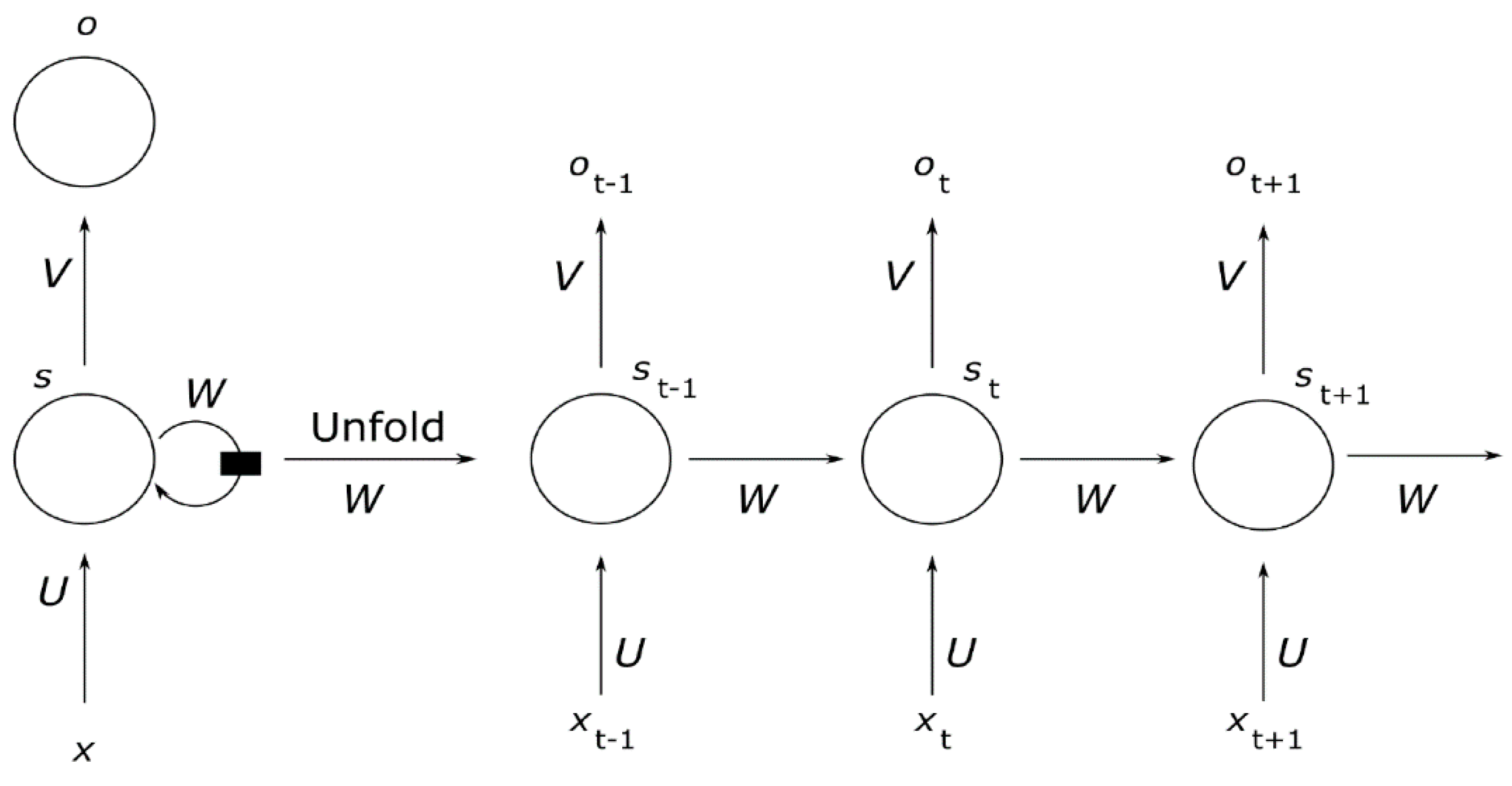
An RNN model is an extension of a feedforward neural network (FFN), which consists of edges that span the adjacent time steps to denote time in the model. The basic difference between an FFN and an RNN is that an RNN does not have cycles among the conventional edges, where this is replaced by adjacent time steps that are recurrent edges. These recurrent edges form cycles that are self-connected by nodes across time. An RNN is a sequential model that consists of memory cells, which act as a hidden state. These memory cells iterate the sequential elements in a loop and maintain its state in vector form, which is known as the state vector [47]. Figure 1 represents the workflow of an RNN model. The current hidden state () is a function of previous hidden state () and the current input (). The value of the current hidden state can be calculated using Equation (1):
where and represents the hidden state values at the current timestep () and the previous timestep (), and the current timestep input value is denoted as . Through a looping mechanism, the output value is fed back into the hidden state to calculate subsequent time steps. Furthermore, an RNN model consists of three hidden nodes having a weight matrix (U, V, W), as shown in Figure 1. The temporal dynamics of an RNN model can be calculated using Equation (2):
The recurrence equation (Equation (2)) filters the weighted sum of inputs and states using a non-mapping activation function. The output value of each time step () contains information about the previous time step and the current time step in a 2D tensor, which is carried forward to the next subsequent time step to form recurrent edges.
In Equation (2), and denote the activation functions at the inputs and output, respectively. The selection of these activation functions depends upon the problem statement. The interested reader can find more details about this model in Lipton et al. [48].
2.2. Long Short-Term Memory (LSTM)
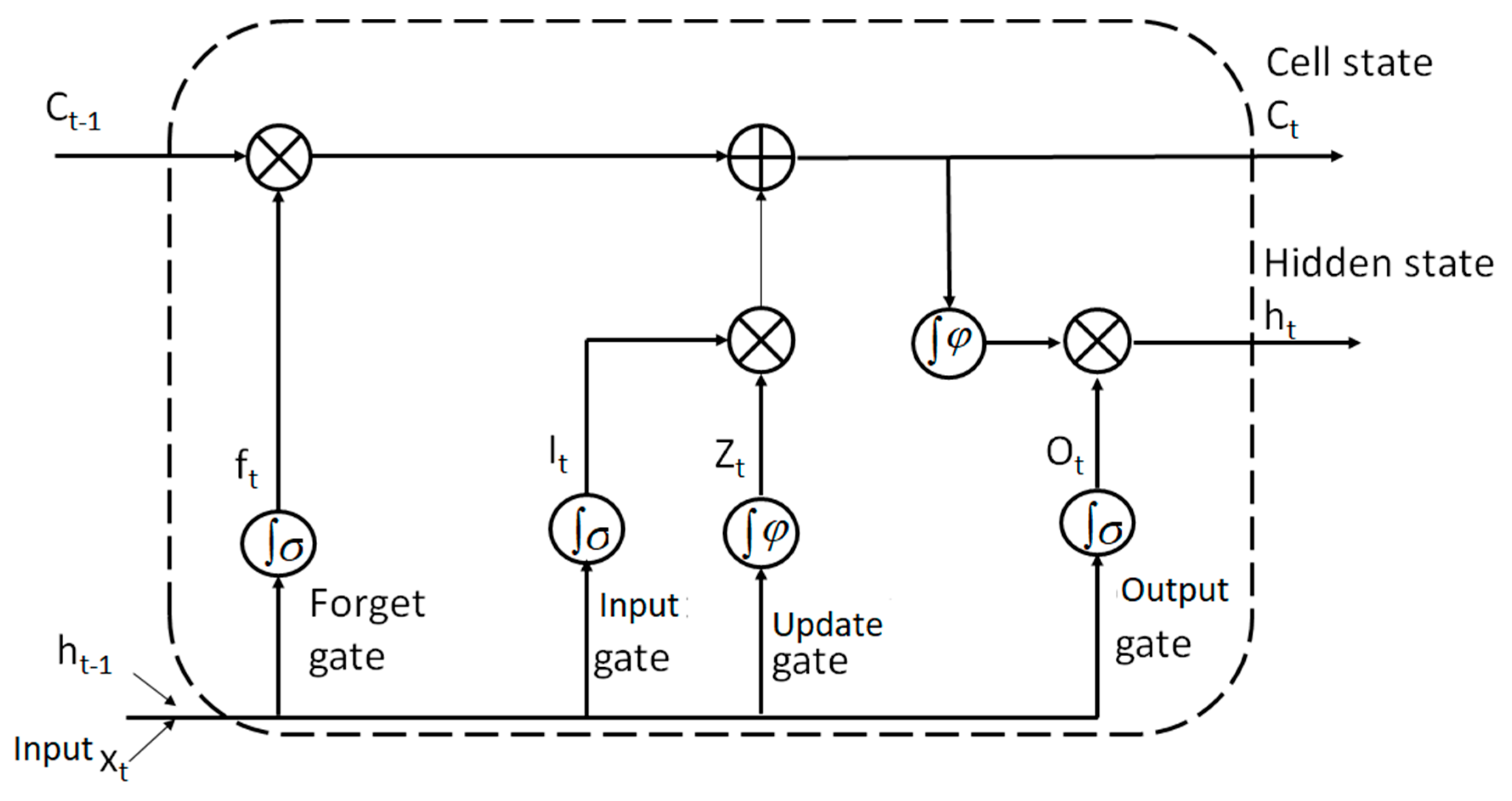
An LSTM is a variant of an RNN architecture proposed by Hochreiter and Schmidhuber that was developed to model sequences and long-term dependencies more precisely than an RNN [49]. The gating mechanism enables an LSTM model to regulate information across the network to overcome the problem of exploding and vanishing gradients [50]. The architecture of a single LSTM block is shown in Figure 2.
The memory block of an LSTM model consists of four units: input gate, forget gate, carry state, and output gate, which regulate the temporal relationship of the previous time series values by remembering or forgetting. The input gate () and forget gate () regulate how much information passes through the current cell and how much information is to be forgotten from the previous memory (), the carry state () modulates the writing of new information to the next memory cell (), and the output gate () decides how much information will pass to the next cell from the current cell. The workflow and gating mechanism of this process is presented in Equation (3):
where c, f, i, and o denote the carry state and the forget, input, and output gates, respectively.
The hidden state (g) present in the memory cell is assessed by the current input () and the previous hidden state (). The forget gate replaces the previous memory with the new input, whereas the hidden state () is considered after the multiplication of and . More details can be found in Bandara et al. [51].
2.3. Genetic Algorithm (GA)
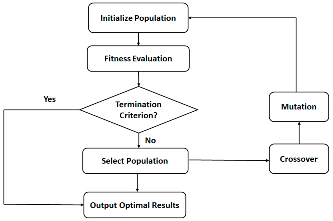
A GA is a natural-evolution-inspired stochastic optimization technique, which is one of the most commonly applied metaheuristic algorithms [52]. A GA process includes evolutionary principles, such as crossover and mutations of chromosomes. Each chromosome behaves as an individual solution to the target problem, which is articulated in a binary string form. The initial population of chromosomes is generated randomly, and the one that gives a better solution to an assigned target is chosen to reproduce [53].
The whole process of optimization is divided into six stages: initialization, fitness calculation, termination via a condition check, selection, crossover, and mutation. Figure 3 denotes the detailed process of a GA. During the process of fitness estimation, only the chromosomes displaying an excellent performance are preserved for further reproduction. This selection and reproduction process is iterated several times to obtain a high probability of superior chromosomes. In the next step, the superior chromosomes generate offspring by interchanging string parts and gene combinations during the crossover process, which results in a new solution. In the mutation process, one of the chromosomes is selected to change a randomly selected bit through arbitrary swapping. The fitness of the generated solution is estimated and checked against the termination criteria. When the termination criteria have been satisfied, the GA process terminates.
2.4. Genetic Algorithm Long Short-Term Memory (GA-LSTM)
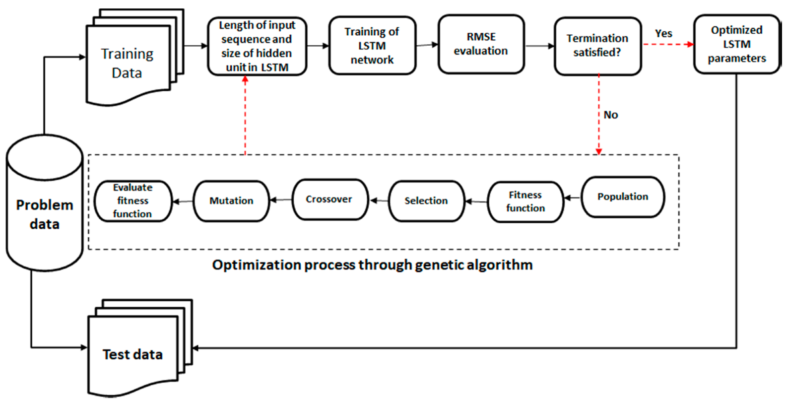
This section describes the hybrid approach of an LSTM sequential model integrated with a GA to find the customized window size and number of units (memory cell) in an LSTM model for water temperature time-series predictions. Since the performance of sequential models (i.e., LSTM) relies on past information from the training phase, the selection of an appropriate or optimized time window plays a vital role in obtaining a more accurate model. For example, if the window is small, there is a chance of important information being neglected, and on the other hand, if the window time is large, the model will overfit during the learning process. Figure 4 shows the flow diagram of the GA-LSTM model used in this study. The learning process consisted of two stages. The first stage was used to design the appropriate network parameters for the LSTM model. To keep the architecture simple, we adopted a single hidden layer, and the optimum number of memory cell units was searched for by the GA. The hyperbolic tangent function was used as an activation function at the inputs and hidden nodes to scale the inputs between −1 and 1, and a linear output function was used as the activation. Furthermore, to adjust the initialized random weight of the network, a gradient-based Adam optimizer was used [54].
In the second stage, to obtain the optimal window size and network parameters, an evolutionary GA was used. The population of chromosomes with a possible solution was initialized with random values. The generated chromosomes were encoded in binary bits, which represented the size of the window and the number of memory cells. The solution of the model was evaluated based on the pre-defined fitness function (RMSE) and strings with a higher performance were retained for reproduction. If the termination criteria were satisfied, the near-optimal solution was calculated by the model. The performance of the model was dependent upon the population size, crossover rate, and mutation rate. In this research, the population size, crossover rate, and mutation rate were selected to be 4, 0.7, and 0.15, respectively. Furthermore, for the stopping condition, the total number of generations was selected to be 10. Pseudo-code of the GA-LSTM is shown in Algorithm 1.
| Algorithm 1: GA-optimized LSTM |
|
3. Research Data and Methods
3.1. Description of the Data Used
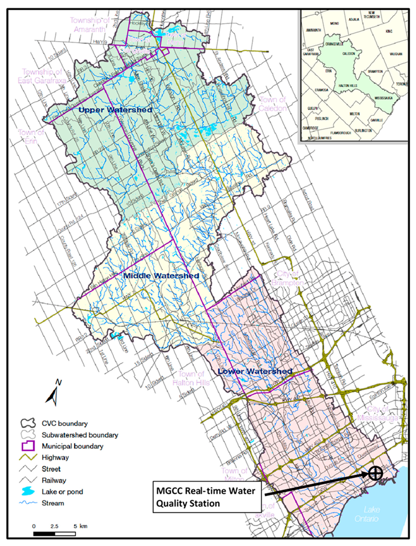
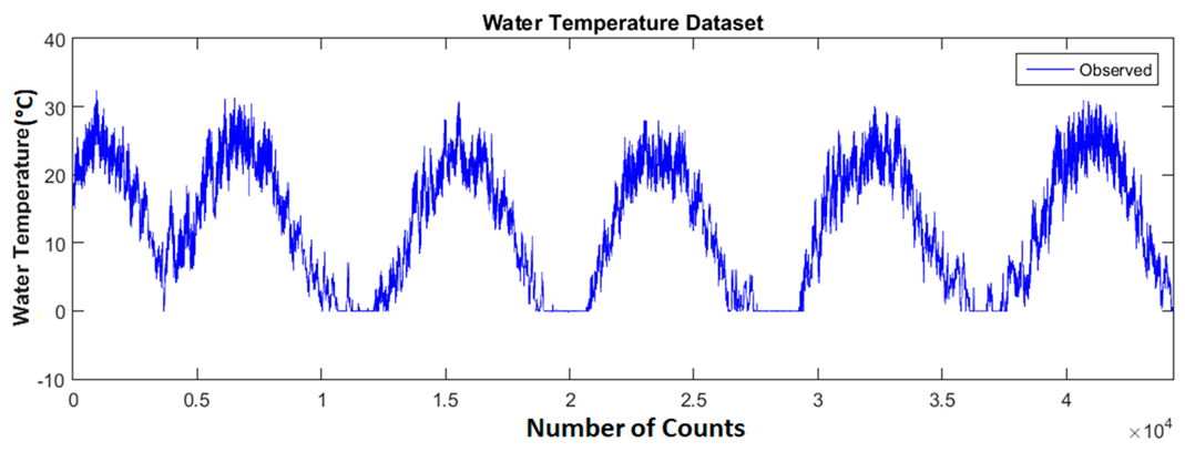
The Credit Valley Conservation Authority (CVC) operates a network of real-time water quality monitoring stations within the Credit River watershed. Temperature data from the Mississauga Golf and Country Club (MGCC) station located in Mississauga, Ontario (43°33′17.2″ N, 79°37′12.9″ W), was chosen for this study (Figure 5). This station is located on the lower Credit River, approximately 3.5 km upstream from Lake Ontario. The Credit River watershed has an area of 1000 square kilometers with land use comprising 31% urban, 34% agriculture and open space, and 35% natural areas [55]. At this point, the Credit River has a mean discharge of 8.1 m3/s according to the Water Survey of Canada station 02HB002 (Credit River at Erindale), which was operational from 1945 to 1993. The water quality was monitored using a Hydrolab DS5X multiparameter sonde. The temperature sensor in the sonde was a variable resistance thermistor with an accuracy of ±0.1 °C and a resolution of 0.01 °C. Sensor data was polled every 15 min and transferred via the intelligent SODATM telemetry platform to a central database. The water temperature sensor was housed within a perforated pipe mounted to a bridge pier. The Credit River is 2 to 3 m deep in winter months at this station. The depth of the sonde was positioned such that the sonde was submerged during low flows. Over the winter, this would normally be below any potential ice cover if it had occurred. This watershed is heavily urbanized and large amounts of road salt are used on roads and parking lots for winter de-icing operations. High chloride concentrations prevent the formation of ice in urban streams. The CVC data quality and validation procedures removed periods where the data was not reliable. The Hydrolab sonde was exchanged monthly for calibration and quality assurance/quality control (QA/QC) validation of the data. Figure 6 shows the time series of the water temperatures.
3.2. Model Development, Performance Assessment, and Forecast Quality Metrics
This section describes the model development of the GA-LSTM and RNN models. To achieve the stated objectives, fully connected RNN and LSTM models were developed for the water temperature modeling using the raw data. The model proposed here was an ensemble of time delay sequential modeling. The RNN and GA-LSTM models were built in TensorFlow using “Keras: The Python Deep Learning library” [57,58]. Since this study formulated the water temperature prediction as a sequence prediction, we adopted the historical data to predict the future temperature.
The investigation also focused on determining how long the historical data (previous time steps) could be used to predict future temperatures. The architecture of the LSTM model consisted of the number of LSTM layers (lr), a fully connected layer (lfc), and the number of hidden units (units_r), which determined the complete structure of the LSTM of the network. Considering all the above aspects, we first designed the simplest layered LSTM model. We fixed lr and lfc to be 1, while units_r was determined through optimization. Once the structure was determined, there were still unknown model parameters that were required to train the model, i.e., the learning rate, batch size, optimizer, and activation function. The determination of these control parameters heavily depends upon the skill and experience of researchers. The conventional optimization method uses stochastic gradient descent (SGD), which is a batch version of the gradient descent that helps to speed up the convergence of the network during the learning process.
Kingma and Ba have developed the Adam optimizer, which adds an adaptive learning rate parameter for the training of large-scale neural networks, where it was found that Adam is more robust than SGD [54]. We used the Adam optimizer with a default learning rate of 0.001 in all our experiments, with a batch size of 10. We chose the ReLu activation function, which has been the subject of some recent attention and has shown significant improvement in terms of performance [59]. The optimal window size and units_r were selected based on the root mean square error of the validation set, which was used as the fitness function for the GA. Setting the GA consisted of a binary representation of a solution of length 10, which was randomly initialized using the Bernoulli distribution [60].
The final setting for the GA was population size = 4, number of generations = 2, and gene length = 10, which was used to obtain the best window and units_r by considering five-fold cross-validation. The elitism technique was utilized to obtain the best solution from the population pool, which was then passed on to the next generation; further iterations of this process took place until the termination criteria were satisfied. The division of the data into training and testing sets varies with the problem of interest. Many researchers in the past have used different divisions: Kurup and Dudani adopted 63% of the available data used for training [61], Boadu used 80% of the available data for training [62], Coulibaly and Baldwin used 90% of the data for training [63], and Pal used 69% of the available data for training [64]. In this study, the entire dataset was divided into a training set (first 90% of the whole, where 20% was taken for validation) and a testing set (last 10% of the whole data set).
In general, the performance of the model was assessed using the minimum prediction error criteria. To evaluate the performance of the developed model, two types of forecasting quality metrics were selected since both correlation and variance affect a model’s performance. Type 1 errors account for the accuracy of the mean and the closeness of the forecasted time series to the target time series, while type 2 errors account for the closeness of the forecasted mean to the mean of the target values. Therefore, we used the coefficient of determination (r2), mean absolute error (MAE), root mean square error (RMSE), ratio of the RMSE to the standard deviation (RSR), modified Nash–Sutcliffe efficiency coefficient (mNSE), modified index of agreement (md), and Kling–Gupta efficiency (KGE) as fitness indices to evaluate the models’ performances (Equations (4)–(9)):
where is the ith hourly water temperature estimated using the models, is the ith observed hourly water temperature, is the average of the estimated hourly water temperature, is the average of the observed hourly water temperature, is the number of observations, and is the standard deviation of the observed hourly water temperature.
The Kling–Gupta efficiency is calculated as follows:
where is the Pearson product-moment correlation coefficient; and , , and are the scaling factors used for re-scaling the criteria space before computing the Euclidean distance. The factor represents the bias ( and represents the variability between the estimated and observed values (.
4. Results and Discussion
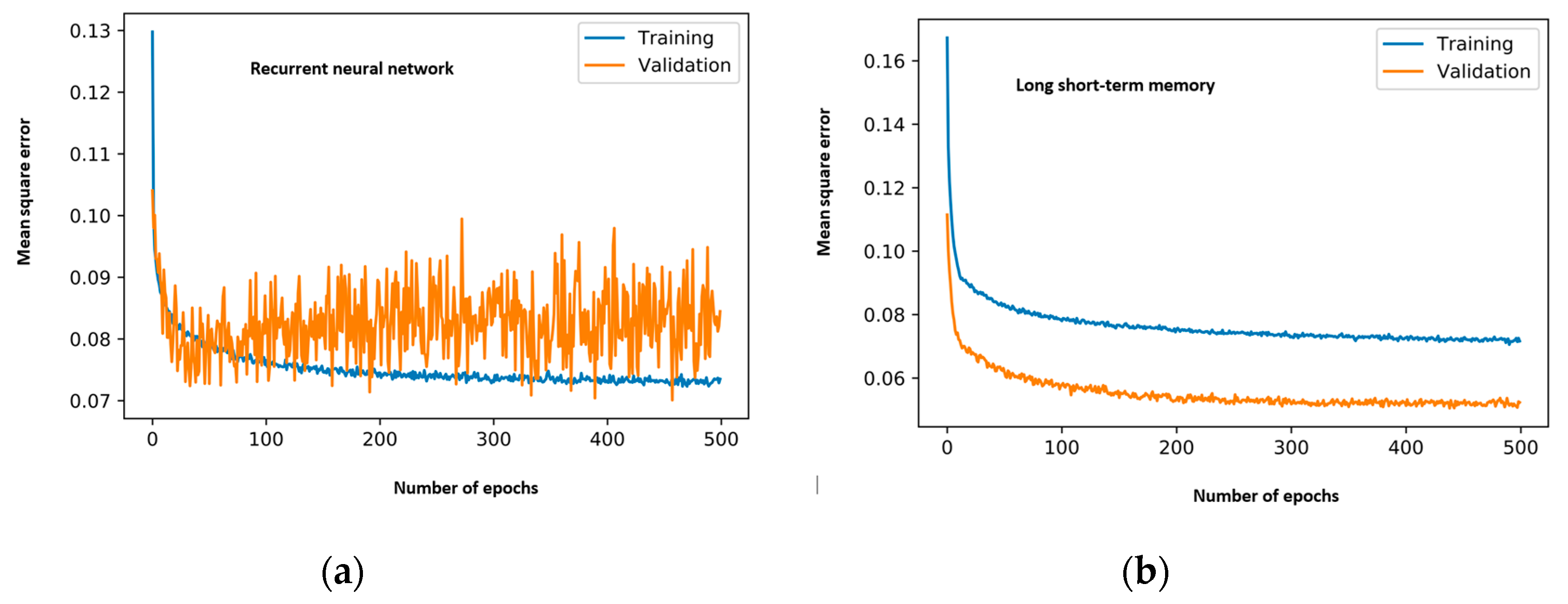
Table 1 shows the optimal window size and the number of units of the memory cell searched by the GA based on the lowest RMSE. The best window size (34) and number of units (9) were used to train the model. In addition, we trained the RNN models with a similar model architecture to compare their performances. Figure 7 shows the plot of the mean square error for the models during the training and validation period.
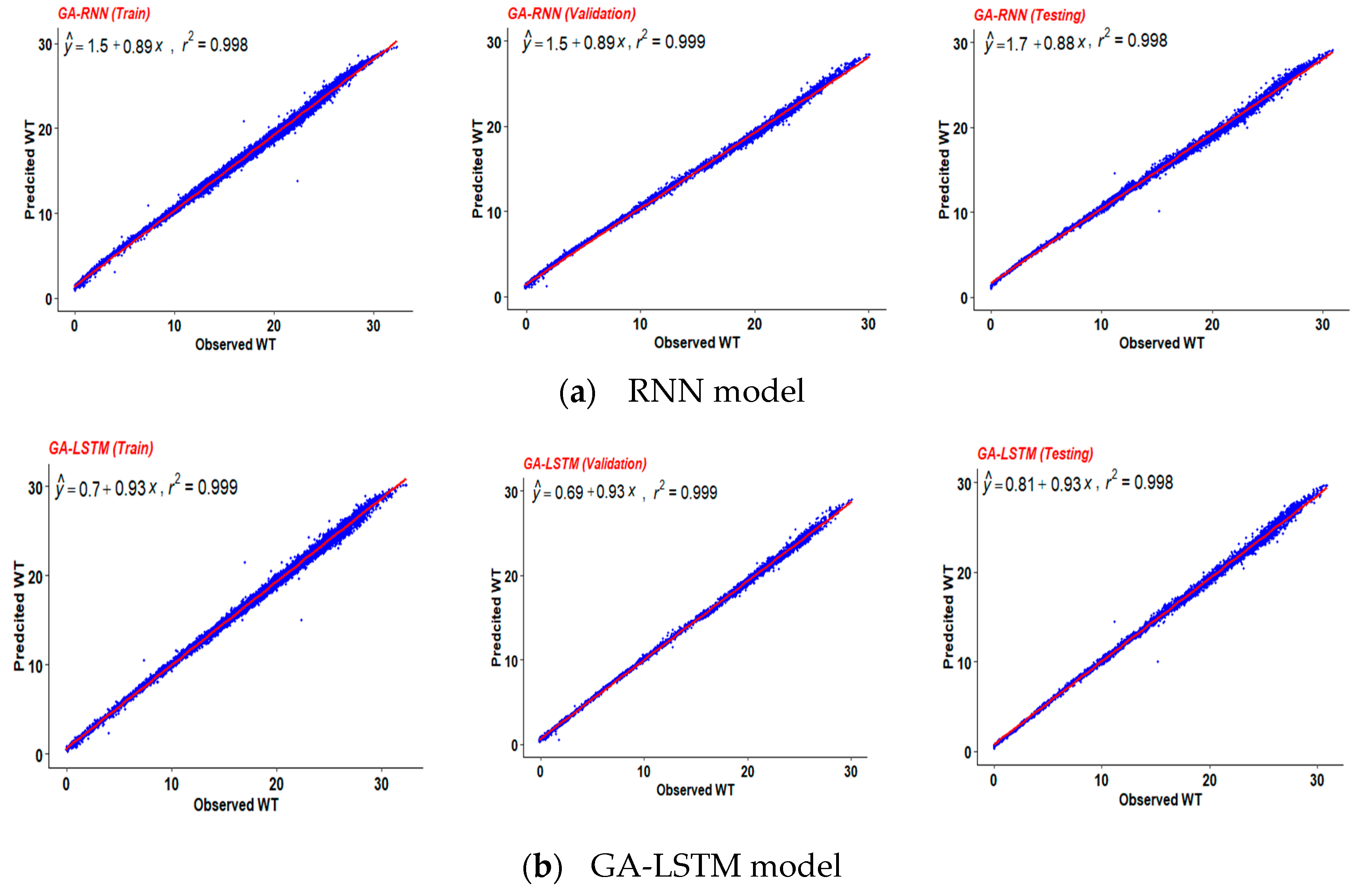
From the analysis, it was evident that the models were well trained as the model performance did not improve as the number of epochs increased. Moreover, the mean square error for the RNN model had inherent noise while converging during the validation period. From this finding, we could conclude that the LSTM model had a better gradient flow for longer time steps than the RNN model and had an improved performance for long-term dependency tasks. The performance of both models was tested by considering the forecast quality metrics (Table 2). As mentioned above, two types of errors were evaluated for both models. Slightly higher coefficients of determination were recorded for the GA-LSTM (r2 = 0.999) than the RNN (r2 = 0.998) during the training period, whereas during validation and testing, both the models showed similar performances.
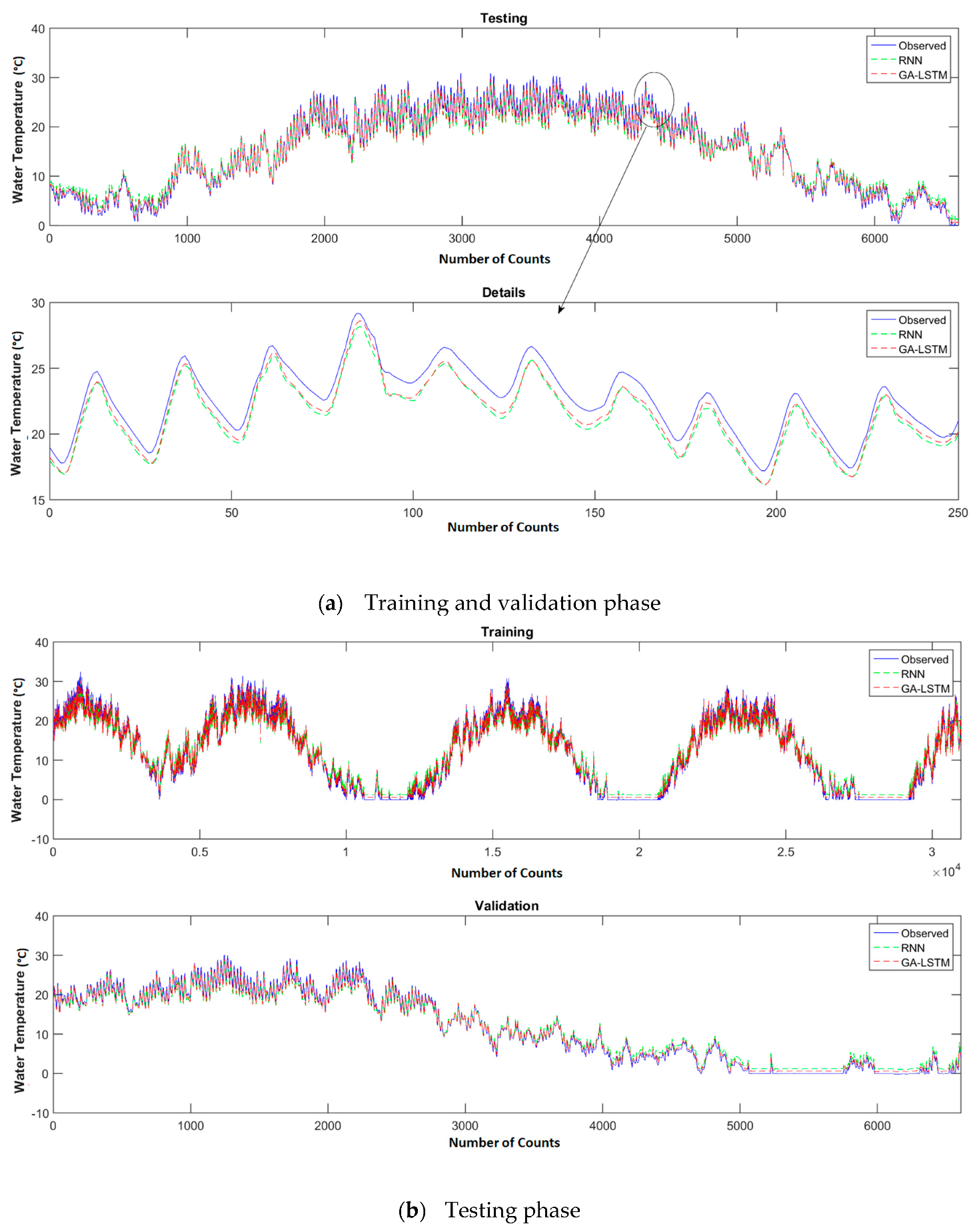
A scatter plot was drawn for better visualization for both the models for the three phases (Figure 8a,b). Furthermore, the performance of other metrics clearly created a distinction between the two models; in terms of RMSE, smaller values were found for the GA-LSTM compared to the RNN in all three phases. In general, the lower the error, the better the model, where the GA-LSTM model showed a smaller error (RMSE = 0.755, RSR = 0.093) than the RNN (RMSE = 1.07, RSR = 0.131) during the testing phase. In addition, the KGE was also calculated to assess the relative importance of the three components (correlation, bias, and variability), while also providing a decomposition of NSE and MSE, which comes under the type 2 error category [65]. Based on these fitness metrics, the GA-LSTM model outperformed the RNN model during all three phases (Table 2). The superior performance of the GA-LSTM model was supported by the modified index of agreement (md), which also showed the highest values. Figure 9a shows that both models were well trained during the training and validation periods and the GA-LSTM model was very capable of forecasting the diurnal temperature peaks. In Figure 8b, it can be easily seen that the GA-LSTM model was good enough for the prediction of water temperature.
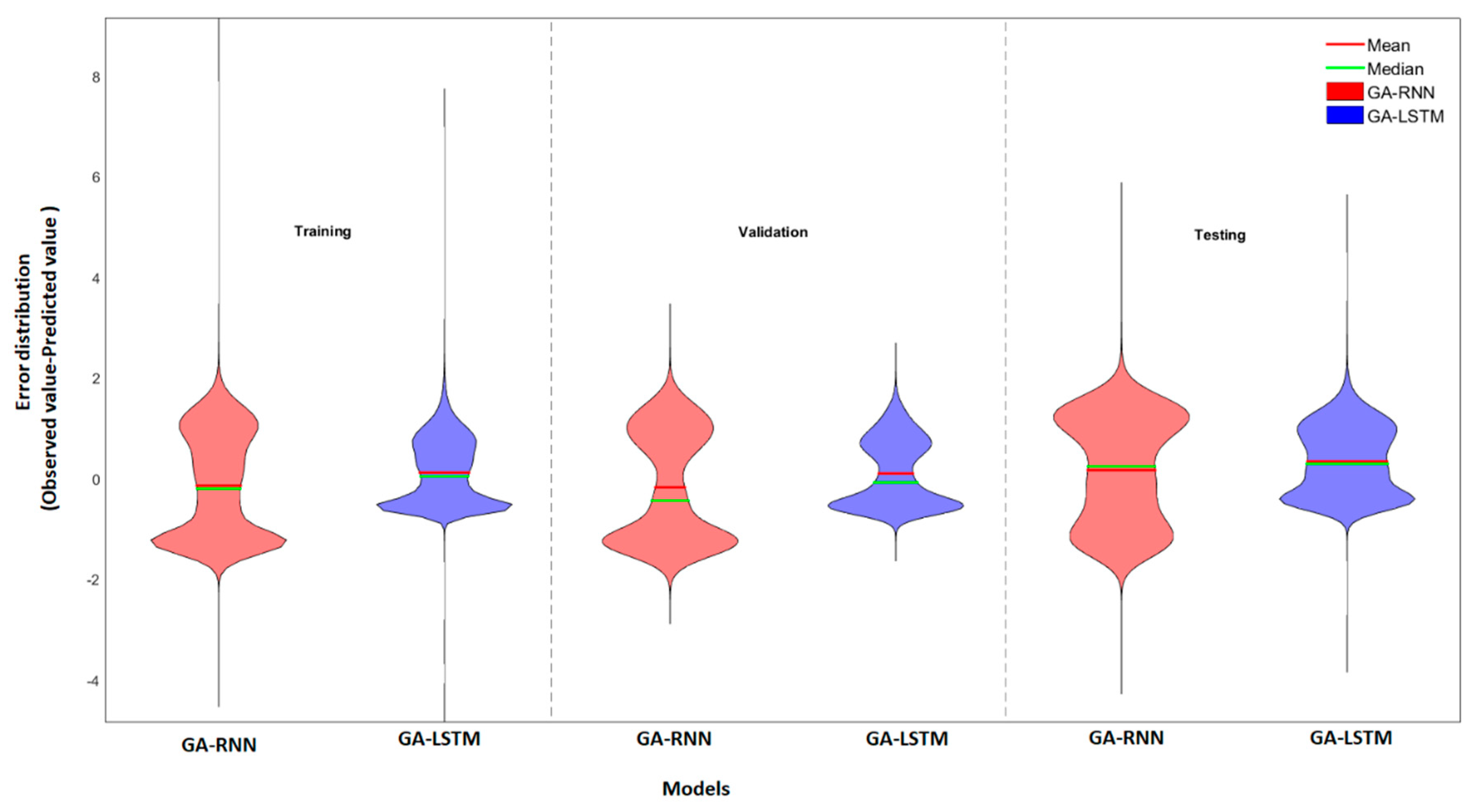
A violin plot is used to visualize the distribution of the error and the probability density produced by models [66]. Its summary statistics show the mean/median and interquartile ranges with a full distribution of the error produced. Figure 10 shows that the RNN model had more outliers and its distribution of error occurred more in the lower quantile range, which was in contrast to the GA-LSTM, where the errors were approximately equally distributed in the upper and lower quantiles. Therefore, it can be concluded that the GA-LSTM model performed better and the selection of the optimal window and number of units by the genetic search was validated. This research finding concluded that GA-LSTM can be used as a better option compared with an RNN and even an LSTM.
5. Concluding Remarks
This study addressed the applicability of a genetic algorithm integrated with an LSTM model (GA-LSTM) to forecast river water temperatures and to solve the long-standing problem of determining the optimal number of memory units and the window size. The LSTM network used in this study was composed of a single layer with nine memory units that utilized 34 previous time steps to forecast a one-step-ahead value. To validate the effectiveness of this approach, a benchmark model (RNN) with the same input configuration was tested as a comparative study. To further test the robustness, different forecast quality metrics were tested. The overall result demonstrated that a GA-LSTM approach can be an effective method for time series analysis and can capture all the features during learning.
This study suggests that a GA-LSTM can help in designing the architecture of an LSTM and its variants for the detection of temporal patterns in data. Future research in this regard can include other tuning parameters of an LSTM model for prediction performance that depends upon other hyperparameters. Further testing and setting of control parameters of the GA, such as the crossover and mutation parameters, can also be improved to enhance model performance.
The application of these deep learning techniques is encouraged since such models present the possibility of exploiting the benefit of understanding the temporal relationships and sequential nature of time series, which in turn helps in achieving higher accuracies.
This research focused on the use of hybrid and series decomposition techniques to improve forecasting accuracy. The proposed GA-LSTM framework achieved a significant forecasting accuracy in comparison with a benchmark RNN model when applied to the water temperature dataset. From the analysis of the results, it was evident that the GA-LSTM model can be a good replacement without compromising accuracy.
The development of real-time water quality monitoring networks for predicting and detecting toxic spills and other adverse events is a potential application for the use of the GA-LSTM framework proposed in this paper [67,68,69,70]. As more urban watercourses become instrumented, fast and effective forecasting tools will be required to predict and respond to adverse water quality events.
Author Contributions
Conceptualization, S.S. and B.G.; methodology, S.S. and D.K.; software, D.K.; validation, S.S., H.B., P.S., and D.K.; formal analysis, S.S. and P.S.; resources, S.S. and B.G.; data curation, S.S.; writing—original draft preparation, S.S. and D.K.; writing—review and editing, S.S., B.G., and H.B.; visualization, S.S. and D.K.; supervision, B.G. and H.B.; funding acquisition, B.G. All authors have read and agreed to the published version of the manuscript.
Funding
This research was funded by the Natural Sciences and Engineering Research Council of Canada (NSERC) Discovery Grant (#400675) and was in partnership with an Ontario Ministry of Transportation Grant (#050235).
Acknowledgments
The river temperature data was generously provided by the Credit Valley Conservation Authority.
Conflicts of Interest
The authors declare no conflict of interest.
References
- Booth, D.B.; Jackson, C.R. Urbanization of aquatic systems: Degradation thresholds, stormwater detection, and the limits of mitigation. J. Am. Water Resour. Assoc. 1997, 33, 1077–1090. [Google Scholar] [CrossRef]
- Walsh, C.J.; Roy, A.H.; Feminella, J.W.; Cottingham, P.D.; Groffman, P.M.; Morgan, R.P. The urban stream syndrome: Current knowledge and the search for a cure. J. N. Am. Benthol. Soc. 2005, 24, 706–723. [Google Scholar] [CrossRef]
- Grimm, N.B.; Faeth, S.H.; Golubiewski, N.E.; Redman, C.L.; Wu, J.; Bai, X.; Briggs, J.M. Global Change and the Ecology of Cities. Science 2008, 319, 756–760. [Google Scholar] [CrossRef] [Green Version]
- Booth, D.B.; Roy, A.H.; Smith, B.; Capps, K.A. Global perspectives on the urban stream syndrome. Freshw. Sci. 2016, 35, 412–420. [Google Scholar] [CrossRef] [Green Version]
- Klein, R.D. Urbanization and stream quality impairment. J. Am. Water Resour. Assoc. 1979, 15, 948–963. [Google Scholar] [CrossRef]
- Wang, L.; Lyons, J.; Kanehl, P. Impacts of Urban Land Cover on Trout Streams in Wisconsin and Minnesota. Trans. Am. Fish. Soc. 2003, 132, 825–839. [Google Scholar] [CrossRef]
- Wallace, A.M.; Croft-White, M.V.; Moryk, J. Are Toronto’s streams sick? A look at the fish and benthic invertebrate communities in the Toronto region in relation to the urban stream syndrome. Environ. Monit. Assess. 2013, 185, 7857–7875. [Google Scholar] [CrossRef] [PubMed]
- Poole, G.C.; Berman, C.H. An Ecological Perspective on In-Stream Temperature: Natural Heat Dynamics and Mechanisms of Human-Caused Thermal Degradation. Environ. Manag. 2001, 27, 787–802. [Google Scholar] [CrossRef]
- Hester, E.T.; Doyle, M.W. Human Impacts to River Temperature and Their Effects on Biological Processes: A Quantitative Synthesis1. JAWRA J. Am. Water Resour. Assoc. 2011, 47, 571–587. [Google Scholar] [CrossRef]
- Somers, K.A.; Bernhardt, E.S.; Grace, J.B.; Hassett, B.A.; Sudduth, E.B.; Wang, S.; Urban, D.L. Streams in the urban heat island: Spatial and temporal variability in temperature. Freshw. Sci. 2013, 32, 309–326. [Google Scholar] [CrossRef] [Green Version]
- Sahoo, G.B.; Schladow, S.G.; Reuter, J.E. Forecasting stream water temperature using regression analysis, artificial neural network, and chaotic non-linear dynamic models. J. Hydrol. 2009, 378, 325–342. [Google Scholar] [CrossRef]
- Bernhardt, E.S.; Heffernan, J.B.; Grimm, N.B.; Stanley, E.H.; Harvey, J.W.; Arroita, M.; Appling, A.P.; Cohen, M.J.; McDowell, W.H.; Hall, R.O.; et al. The metabolic regimes of flowing waters. Limnol. Oceanogr. 2018, 63, S99–S118. [Google Scholar] [CrossRef] [Green Version]
- Rossi, L.; Hari, R.E. Screening procedure to assess the impact of urban stormwater temperature to populations of brown trout in receiving water. Integr. Environ. Assess. Manag. 2007, 3, 383–392. [Google Scholar] [CrossRef] [PubMed]
- Armour, C.L. Guidance for Evaluating and Recommending Temperature Regimes to Protect Fish; US Department of the Interior, Fish and Wildlife Service: Bailey’s Crossroads, VA, USA, 1991; Volume 90.
- Steedman, R.J. Occurrence and Environmental Correlates of Black Spot Disease in Stream Fishes near Toronto, Ontario. Trans. Am. Fish. Soc. 1991, 120, 494–499. [Google Scholar] [CrossRef]
- Hasnain, S.S.; Minns, C.K.; Shuter, B.J.; Temperature, K.E.; Fishes, F. Key Ecological Temperature Metrics for Canadian Freshwater Fishes; Ontario Forest Research Institute: Sault Ste. Marie, ON, Canada, 2010. [Google Scholar]
- COSEWIC. COSEWIC Assessment and Update Status Report Clinostomus Elongatus in Canada; Committee on the Status of Endangered Wildlife in Canada: Ottawa, ON, Canada, 2007. [Google Scholar]
- Benyahya, L.; Caissie, D.; St-Hilaire, A.; Ouarda, T.B.M.J.; Bobée, B. A Review of Statistical Water Temperature Models. Can. Water Resour. J. 2007, 32, 179–192. [Google Scholar] [CrossRef] [Green Version]
- Stefan, H.G.; Preud’homme, E.B. Stream temperature estimation from air temperature. J. Am. Water Resour. Assoc. 1993, 29, 27–45. [Google Scholar] [CrossRef]
- Johnson, S.L. Stream temperature: Scaling of observations and issues for modelling. Hydrol. Process. 2003, 17, 497–499. [Google Scholar] [CrossRef]
- Arismendi, I.; Safeeq, M.; Dunham, J.B.; Johnson, S.L. Can air temperature be used to project influences of climate change on stream temperature? Environ. Res. Lett. 2014, 9, 084015. [Google Scholar] [CrossRef]
- Leach, J.A.; Moore, R.D. Empirical Stream Thermal Sensitivities May Underestimate Stream Temperature Response to Climate Warming. Water Resour. Res. 2019, 55, 5453–5467. [Google Scholar] [CrossRef]
- Somers, K.A.; Bernhardt, E.S.; McGlynn, B.L.; Urban, D.L. Downstream Dissipation of Storm Flow Heat Pulses: A Case Study and its Landscape-Level Implications. JAWRA J. Am. Water Resour. Assoc. 2016, 52, 281–297. [Google Scholar] [CrossRef]
- Bartholow, J.M. Stream Temperature Investigations: Field and Analytic Methods; Instream Flow Information Paper No. 13; US Department of the Interior, Fish and Wildlife Service: Bailey’s Crossroads, VA, USA, 1989.
- Caisse, D. The thermal regime of rivers: A review. Freshw. Biol. 2006, 51, 1389–1406. [Google Scholar] [CrossRef]
- Janke, B.D.; Herb, W.R.; Mohseni, O.; Stefan, H.G. Application of a Runoff Temperature Model (HTSim) to a Residential Development in Plymouth, MN; St. Anthony Falls Laboratory: Minneapolis, MN, USA, 2007. [Google Scholar]
- Webb, B.W.; Hannah, D.M.; Moore, R.D.; Brown, L.E.; Nobilis, F. Recent advances in stream and river temperature research. Hydrol. Process. 2008, 22, 902–918. [Google Scholar] [CrossRef]
- Wool, T.; Ambrose, R.; Martin, J. WASP8 Temperature Model Theory and User’s Guide; US EPA: Washington, DC, USA, 2008.
- Dugdale, S.J.; Hannah, D.M.; Malcolm, I.A. River temperature modelling: A review of process-based approaches and future directions. Earth Sci. Rev. 2017, 175, 97–113. [Google Scholar] [CrossRef]
- Cole, T.M.; Wells, S.A. CE-QUAL-W2: A Two-Dimensional, Laterally Averaged, Hydrodynamic and Water Quality Model, Version 4.2; U.S. Army Corps of Engineers: Washington, DC, USA, 2019.
- Chenard, J.-F.; Caissie, D. Stream temperature modelling using artificial neural networks: Application on Catamaran Brook, New Brunswick, Canada. Hydrol. Process. 2008, 22, 3361–3372. [Google Scholar] [CrossRef]
- Liu, W.C.; Chen, W.B. Prediction of water temperature in a subtropical subalpine lake using an artificial neural network and three-dimensional circulation models. Comput. Geosci. 2012, 45, 13–25. [Google Scholar] [CrossRef]
- Piotrowski, A.P.; Napiorkowski, M.J.; Napiorkowski, J.J.; Osuch, M. Comparing various artificial neural network types for water temperature prediction in rivers. J. Hydrol. 2015, 529, 302–315. [Google Scholar] [CrossRef]
- Liu, S.; Xu, L.; Li, D. Multi-scale prediction of water temperature using empirical mode decomposition with back-propagation neural networks. Comput. Electr. Eng. 2016, 49, 1–8. [Google Scholar] [CrossRef]
- Piccolroaz, S.; Calamita, E.; Majone, B.; Gallice, A.; Siviglia, A.; Toffolon, M. Prediction of river water temperature: A comparison between a new family of hybrid models and statistical approaches. Hydrol. Process. 2016, 30, 3901–3917. [Google Scholar] [CrossRef]
- Ebtehaj, I.; Bonakdari, H.; Moradi, F.; Gharabaghi, B.; Khozani, Z.S. An integrated framework of Extreme Learning Machines for predicting scour at pile groups in clear water condition. Coast. Eng. 2018, 135, 1–15. [Google Scholar] [CrossRef]
- Gazendam, E.; Gharabaghi, B.; Ackerman, J.D.; Whiteley, H. Integrative neural networks models for stream assessment in restoration projects. J. Hydrol. 2016, 536, 339–350. [Google Scholar] [CrossRef]
- Ghorbani, M.A.; Shamshirband, S.; Zare Haghi, D.; Azani, A.; Bonakdari, H.; Ebtehaj, I. Application of firefly algorithm-based support vector machines for prediction of field capacity and permanent wilting point. Soil Tillage Res. 2017, 172, 32–38. [Google Scholar] [CrossRef]
- Bonakdari, H.; Moeeni, H.; Ebtehaj, I.; Zeynoddin, M.; Mahoammadian, A.; Gharabaghi, B. New insights into soil temperature time series modeling: Linear or nonlinear? Theor. Appl. Clim. 2019, 135, 1157–1177. [Google Scholar] [CrossRef]
- Sabouri, F.; Gharabaghi, B.; Perera, N.; McBean, E. Evaluation of the Thermal Impact of Stormwater Management Ponds. J. Water Manag. Model. 2013, 246–258. [Google Scholar] [CrossRef] [Green Version]
- Sabouri, F.; Gharabaghi, B.; McBean, E.; Tu, C. Thermal Investigation of Stromwater Management Ponds. J. Water Manag. Model. 2016. [Google Scholar] [CrossRef] [Green Version]
- Sabouri, F.; Gharabaghi, B.; Sattar, A.M.A.; Thompson, A.M. Event-based stormwater management pond runoff temperature model. J. Hydrol. 2016, 540, 306–316. [Google Scholar] [CrossRef]
- Sattar, A.M.A.; Gharabaghi, B.; Sabouri, F.; Thompson, A.M. Urban stormwater thermal gene expression models for protection of sensitive receiving streams. Hydrol. Process. 2017, 31, 2330–2348. [Google Scholar] [CrossRef]
- Bedi, J.; Toshniwal, D. Empirical Mode Decomposition Based Deep Learning for Electricity Demand Forecasting. IEEE Access 2018, 6, 49144–49156. [Google Scholar] [CrossRef]
- Zhang, Q.; Wang, H.; Dong, J.; Zhong, G.; Sun, X. Prediction of Sea Surface Temperature Using Long Short-Term Memory. IEEE Geosci. Remote Sens. Lett. 2017, 14, 1745–1749. [Google Scholar] [CrossRef] [Green Version]
- Kumar, D.; Singh, A.; Samui, P.; Jha, R.K. Forecasting monthly precipitation using sequential modelling. Hydrol. Sci. J. 2019, 64, 690–700. [Google Scholar] [CrossRef]
- LeCun, Y.; Bengio, Y.; Hinton, G. Deep learning. Nature 2015, 521, 436–444. [Google Scholar] [CrossRef]
- Lipton, Z.C.; Berkowitz, J.; Elkan, C. A Critical Review of Recurrent Neural Networks for Sequence Learning. arXiv 2015, arXiv:1506.00019. [Google Scholar]
- Hochreiter, S.; Schmidhuber, J. Long Short-Term Memory. Neural Comput. 1997, 9, 1735–1780. [Google Scholar] [CrossRef] [PubMed]
- Chandar, S.; Sankar, C.; Vorontsov, E.; Kahou, S.E.; Bengio, Y. Towards Non-Saturating Recurrent Units for Modelling Long-Term Dependencies. In Proceedings of the AAAI Conference on Artificial Intelligence, Honolulu, HI, USA, 22 January 2019. [Google Scholar] [CrossRef]
- Bandara, K.; Bergmeir, C.; Smyl, S. Forecasting across time series databases using recurrent neural networks on groups of similar series: A clustering approach. Expert Syst. Appl. 2020, 140, 112896. [Google Scholar] [CrossRef] [Green Version]
- Holland, J.H. Adaptation in Natural and Artificial Systems: An Introductory Analysis with Applications to Biology, Control, and Artificial Intelligence; MIT Press: Cambridge, MA, USA, 1992. [Google Scholar]
- Armano, G.; Marchesi, M.; Murru, A. A hybrid genetic-neural architecture for stock indexes forecasting. Inf. Sci. 2005, 170, 3–33. [Google Scholar] [CrossRef]
- Diederik, K.; Ba, J.L. ADAM: A Method for Stochastic Optimization. AIP Conf. Proc. 2014, 1631, 58–62. [Google Scholar] [CrossRef]
- Credit Valley Conservation (CVC). Integrated Watershed Monitoring Program Biennial Report 2016 and 2017; CVC: Mississauga, ON, Canada, 2019. [Google Scholar]
- Credit Valley Conservation (CVC). Watershed Monitoring: Real-Time Water Quality. Available online: http://www.creditvalleyca.ca/watershed-science/watershed-monitoring/real-time-water-quality/ (accessed on 6 April 2017).
- Abadi, M.; Agarwal, A.; Barham, P.; Brevdo, E.; Chen, Z.; Citro, C.; Corrado, G.S.; Davis, A.; Dean, J.; Devin, M.; et al. TensorFlow: Large-Scale Machine Learning on Heterogeneous Distributed Systems. arXiv 2016, arXiv:1603.04467. [Google Scholar]
- Chollet, F. Keras: The Python Deep Learning Library. 2015. Available online: https://keras.io/ (accessed on 5 June 2019).
- Talathi, S.S.; Vartak, A. Improving performance of recurrent neural network with relu nonlinearity. arXiv 2015, arXiv:1511.03771. [Google Scholar]
- Bodenhofer, U. Genetic Algorithms: Theory and Applications, 2nd ed.; Johannes Kepler Universit: Linz, Austria, 2001. [Google Scholar]
- Kurup, P.U.; Dudani, N.K. Neural Networks for Profiling Stress History of Clays from PCPT Data. J. Geotech. Geoenviron. Eng. 2002, 128, 569–579. [Google Scholar] [CrossRef]
- Boadu, F.K. Rock Properties and Seismic Attenuation: Neural Network Analysis. Pure Appl. Geophys. 1997, 149, 507–524. [Google Scholar] [CrossRef]
- Coulibaly, P.; Baldwin, C.K. Nonstationary hydrological time series forecasting using nonlinear dynamic methods. J. Hydrol. 2005, 307, 164–174. [Google Scholar] [CrossRef]
- Pal, M. Support vector machines-based modelling of seismic liquefaction potential. Int. J. Numer. Anal. Methods Geomech. 2006, 30, 983–996. [Google Scholar] [CrossRef]
- Gupta, H.V.; Kling, H.; Yilmaz, K.K.; Martinez, G.F. Decomposition of the mean squared error and NSE performance criteria: Implications for improving hydrological modelling. J. Hydrol. 2009, 377, 80–91. [Google Scholar] [CrossRef] [Green Version]
- Hintze, J.L.; Nelson, R.D. Violin Plots: A Box Plot-Density Trace Synergism. Am. Stat. 1998, 52, 181–184. [Google Scholar] [CrossRef]
- Glasgow, H.B.; Burkholder, J.M.; Reed, R.E.; Lewitus, A.J.; Kleinman, J.E. Real-time remote monitoring of water quality: A review of current applications, and advancements in sensor, telemetry, and computing technologies. J. Exp. Mar. Biol. Ecol. 2004, 300, 409–448. [Google Scholar] [CrossRef]
- Wang, Z.; Song, H.; Watkins, D.W.; Ong, K.G.; Xue, P.; Yang, Q.; Shi, X. Cyber-physical systems for water sustainability: Challenges and opportunities. IEEE Commun. Mag. 2015, 53, 216–222. [Google Scholar] [CrossRef] [Green Version]
- Fijani, E.; Barzegar, R.; Deo, R.; Tziritis, E.; Skordas, K. Design and implementation of a hybrid model based on two-layer decomposition method coupled with extreme learning machines to support real-time environmental monitoring of water quality parameters. Sci. Total Environ. 2019, 648, 839–853. [Google Scholar] [CrossRef]
- Meyer, A.M.; Klein, C.; Fünfrocken, E.; Kautenburger, R.; Beck, H.P. Real-time monitoring of water quality to identify pollution pathways in small and middle scale rivers. Sci. Total Environ. 2019, 651, 2323–2333. [Google Scholar] [CrossRef]
Figure 1.
Unfolded recurrent neural network (RNN) in time [41].
Figure 1.
Unfolded recurrent neural network (RNN) in time [41].

Figure 2.
Basic architecture of a single long short-term memory (LSTM) block.

Figure 3.
Basic architecture of a genetic algorithm (GA).

Figure 4.
Flow diagram of the GA-LSTM model.

Figure 5.
Location of the Mississauga Golf and Country Club (MGCC) real-time water quality station within the Credit River watershed [56].
Figure 5.
Location of the Mississauga Golf and Country Club (MGCC) real-time water quality station within the Credit River watershed [56].

Figure 6.
Line plot displaying the water temperature time series.

Figure 7.
The performance of the (a) RNN and (b) LSTM models during training and validation.

Figure 8.
Scatter plot displaying the performances of the RNN and GA-LSTM models; the unit used for water temperature (WT) is degrees Celsius.
Figure 8.
Scatter plot displaying the performances of the RNN and GA-LSTM models; the unit used for water temperature (WT) is degrees Celsius.

Figure 9.
Water temperature predictions during the (a) training and validation and (b) testing phases.
Figure 9.
Water temperature predictions during the (a) training and validation and (b) testing phases.

Figure 10.
Water temperature prediction during training and validation.


Table 1.
Selection of optimal window and number of units by GA.
| Cross-Validation | Window Size | No. of Units | MAE |
|---|---|---|---|
| 1 | 28 | 2 | 0.07218 |
| 2 | 14 | 8 | 0.05517 |
| 3 | 44 | 3 | 0.05312 |
| 4 | 42 | 2 | 0.06185 |
| 5 | 34 | 9 | 0.04136 |
MAE: Mean absolute error.
Table 2.
Model performance in terms of different forecast quality metrics.
| Quality Metric | Training | Validation | Testing | |||
|---|---|---|---|---|---|---|
| RNN | GA-LSTM | RNN | GA-LSTM | RNN | GA-LSTM | |
| RMSE (type 1) | 1.049 | 0.654 | 1.097 | 0.467 | 1.07 | 0.755 |
| RSR | 0.118 | 0.073 | 0.119 | 0.072 | 0.131 | 0.093 |
| mNSE | 0.881 | 0.929 | 0.878 | 0.93 | 0.867 | 0.913 |
| md (type 1) | 0.937 | 0.963 | 0.935 | 0.964 | 0.929 | 0.955 |
| r2 | 0.998 | 0.999 | 0.999 | 0.999 | 0.998 | 0.998 |
| KGE (Type 2) | 0.889 | 0.933 | 0.887 | 0.932 | 0.878 | 0.923 |
RMSE: Root mean square error, RSR: Ratio of the RMSE to the standard deviation, mNSE: Modified Nash–Sutcliffe efficiency coefficient, md: Modified index of agreement, and KGE: Kling–Gupta efficiency.
© 2020 by the authors. Licensee MDPI, Basel, Switzerland. This article is an open access article distributed under the terms and conditions of the Creative Commons Attribution (CC BY) license (http://creativecommons.org/licenses/by/4.0/).
Share and Cite
MDPI and ACS Style
Stajkowski, S.; Kumar, D.; Samui, P.; Bonakdari, H.; Gharabaghi, B. Genetic-Algorithm-Optimized Sequential Model for Water Temperature Prediction. Sustainability 2020, 12, 5374. https://doi.org/10.3390/su12135374
AMA Style
Stajkowski S, Kumar D, Samui P, Bonakdari H, Gharabaghi B. Genetic-Algorithm-Optimized Sequential Model for Water Temperature Prediction. Sustainability. 2020; 12(13):5374. https://doi.org/10.3390/su12135374
Chicago/Turabian StyleStajkowski, Stephen, Deepak Kumar, Pijush Samui, Hossein Bonakdari, and Bahram Gharabaghi. 2020. "Genetic-Algorithm-Optimized Sequential Model for Water Temperature Prediction" Sustainability 12, no. 13: 5374. https://doi.org/10.3390/su12135374
Note that from the first issue of 2016, this journal uses article numbers instead of page numbers. See further details here.