
Abstract
The rate-dependent effect of viscoelasticity plays a critical role in the hardening mechanisms of impact-hardening polymers (IHP) when forcefully impacted. In this study, we used dynamic mechanical analysis (DMA) to characterize the rate-dependent viscoelasticity of an IHP under oscillatory shear. We found that the storage modulus increased by three orders of magnitude within the experimental range when the oscillatory frequency varied from 0.1 to 100 rad/s. To further understand the real strain rate effect of IHP, we introduced the Havriliak-Negami (H–N) model to predict the dynamic viscoelastic behaviors of the IHP for a wider frequency range (from zero to infinity) than that applied in the DMA experiments. Based on the H–N model results, we defined a parameter to describe the rate-dependent effect of the IHP, which was not dependent on the frequency range and reflected the intrinsic material properties of IHP. We used the time-temperature superposition principle (TTSP), which extended the experimental range from 0.1 rad s−1 down to 0.005 rad s−1, to verify the accuracy of the rate-dependent viscoelasticity predicted by the H–N model. Finally, we outlined the influence of temperature on the dynamic viscoelastic behaviors of IHP and discussed the phase transition mechanism induced by temperature and the oscillatory frequency. The results presented here not only provide a method (i.e., by combining experimental results with the H–N model results) to characterize the real rate-dependent viscoelasticity of IHP but are also valuable to further our understanding of the impact-hardening mechanisms of IHP.
Export citation and abstract BibTeX RIS

Original content from this work may be used under the terms of the Creative Commons Attribution 4.0 licence. Any further distribution of this work must maintain attribution to the author(s) and the title of the work, journal citation and DOI.
1. Introduction
Impact-hardening polymers (IHPs) are smart materials with viscoelasticity that is very sensitive to the applied loading rate [1–3]—famous commercial examples include Silly Putty® and D3O®. The characteristic relaxation time for a specific IHP is fixed, IHPs behave like an elastic solid when the Deborah number is large (i.e., a short loading time), or like a viscous liquid when the Deborah number is small (i.e., a long loading time) [4]. Most of the loading energy applied to IHPs is absorbed during the stimuli-responsive stage, and thus, they are considered good potential candidate for impact protection [5]. Unlike IHPs' counterparts, shear-thickening liquids [6], leakage is not an issue for IHPs. This advantage extends IHPs' potential applications to include electromechanical sensors [7, 8], lithium anode protection [9], surgery on tympanic cavities [10], and to delay the flow of instabilities in the extrusion of polymers [11], among other uses. However, the underlying impact-hardening mechanisms remain poorly understood and should be explored further to improve the potential of IHPs to provide better impact protection.
Rate-dependent viscoelasticity plays a critical role in the impact-hardening mechanism of IHPs. By quantitatively characterizing the strain rate-dependent viscoelasticity of IHPs, we can determine why IHPs provide better impact protection than conventional polymers, and how IHPs produce a stronger rate-dependent effect. Due to the amorphous state of IHPs, defining their viscoelastic properties over a wide range of strain rates can be challenging when they are under uniaxial compressive or tensile loading. The plasticine-like state of IHPs makes their assembly difficult; for instance, assembling IHPs into columned samples with a large length-to-diameter ratio or dumbbell shapes. Lai et al measured the stress-strain curves of IHPs under different loading speeds across a low strain-rate range (<10−1 s−1) and observed an obvious rate-dependent effect [12]. The drop-hammer test has been widely used to investigate the mechanical behaviors of IHPs within a medium strain-rate range (10−1 s−1 ∼ 102 s−1), the experimental results of which indicate that the strain rate influences the viscoelasticity of IHPs [13, 14]. For higher strain rates (102 s−1 ∼ 104 s−1), the impact-hardening phenomenon can still be observed by using the split Hopkinson pressure bar (SHPB) [15, 16]. However, the viscoelastic properties of IHPs for different strain-rate ranges obtained by the abovementioned methods are difficult to compared, primarily because of the different sample sizes and measurement principles employed in each method. Thus, obtaining comparable viscoelastic data for IHPs across a wide range of strain rates (from quasi-static to medium strain rate to high strain rate) would be very valuable.
Dynamic mechanical analysis (DMA) is a useful technique to investigate the viscoelastic response of an amorphous polymer or complex fluid [17–20]. The rate-dependent viscoelasticity can be equivalently expressed by frequency-dependent dynamic viscoelastic parameters (i.e., storage modulus, loss modulus, and loss factor) determined by DMA in a linear viscoelastic range [21]. The equivalent range of strain rate can be extended from a low strain-rate to a medium strain-rate (10−4 s−1∼100 s−1) by DMA. Thus, DMA can be used to measure the viscoelasticity across a wider range of strain-rate range than other techniques, such as a single device under uniaxial loading mode. Therefore, frequency-dependent dynamic mechanical properties are widely used to evaluate the rate-dependent effect of amorphous polymers [22–24].
To the best of our knowledge, few studies have explored whether the viscoelasticity of IHPs is sensitive to the strain rate beyond the experimental frequency range. Indeed, experimental data alone cannot adequately reveal the rate-dependent effect because the rate-dependency of viscoelasticity of IHPs beyond the experimental range is unknown. To this end, here we introduce a suitable theoretical model to predict the rate-dependent viscoelasticity of IHPs beyond the experimental range. We also explore the influence of temperature on the frequency-dependent dynamic mechanical properties of IHPs [25–27]. We use the time-temperature superposition principle (TTSP) to extend the experimental range to verify the accuracy of the proposed theoretical model. To thoroughly understand the rate-dependent viscoelastic behaviors of IHPs, we study the frequency-dependent dynamic mechanical properties of an IHP (ESA) under oscillatory shear within a linear viscoelastic range. We also discuss the effect of temperature on the dynamic viscoelastic properties. Finally, we propose a new parameter to evaluate the rate-dependent effect of IHPs by combining our results with the results provided by the Havriliak-Negami (H–N) model.
2. Experimental
2.1. Materials
The IHP used in this study, called ESA (figure 1(c)), was provided by Shenzhen Innovation Advanced Materials Co. Ltd, Shenzhen, China. The components of ESA are similar to those of Silly Putty produced by Dow Corning Corporation, which is a type of boric acid-modified polydimethylsiloxane (PDMS). The strain rate effect of ESA is closely related to the pre-existing B–O bonds in ESA. In this study, we primarily focus on a quantitative description of the real rate-dependent viscoelasticity of ESA, the microscopic mechanism is not discussed in detail.

Figure 1. The parallel-plate rheometer (a), schematic of oscillatory shear (b), and the photo of ESA (c).
Download figure:
Standard image High-resolution image2.2. Characterization
We used a parallel-plate rheometer (TA instrument, discovery HR-2) to carry out DMA (figure 1(a)). As shown in figure 1(b), oscillatory shear can be carried out directly using a discovery HR-2 rheometer on a sample of ESA with a geometry of Φ25 mm × 1 mm. The range of oscillatory angular frequency was 10−1 rad s∼102 rad/s, and the temperature was controlled between 20 °C and 200 °C. By implementing a large amplitude oscillatory shear (LAOS), we could determine the linear viscoelastic (LVE) range [28]. We then chose a suitable loading condition to ensure the measurements outlined below were implemented within the LVE range. The shape of the Lissajous curves within each cyclical loading period was monitored in situ using a discovery HR-2 rheometer to evaluate the linear viscoelasticity, thus providing an assistant method. The different loading conditions are shown in the captions of the related figures.
Differential scanning calorimetry was performed using a DSC 8500 (PerkinElmer Inc., USA) with a heating rate of 15 °C min−1 in a nitrogen environment. The temperature range for DSC was set to −50 °C∼200 °C. A TGA 8000 (PerkinElmer Inc., USA) was used to perform thermogravimetric analysis. The heating rate was 15 °C min−1 from 30 °C to 200 °C, and the nitrogen flow was set at 20 ml min−1.
3. Results and discussion
3.1. Determination of LVE range
Within the LVE range, the dynamic viscoelastic moduli, i.e., the storage modulus and the loss modulus, fully describe the viscoelastic response of soft material or complex fluids and are endowed with specific physical meanings [28]. When a sinusoidal strain is applied, the response stress of a linear viscoelastic material is also sinusoidal, with the same oscillatory frequency and a phase shift. In other words, the dynamic viscoelastic moduli are independent of oscillatory strain amplitude within the LVE range [29], which is a valuable criterion to determine the LVE range of viscoelastic materials [30–32]. In this work, we discuss the linear viscoelasticity of ESA and its frequency and temperature dependence. To begin, we determined the LVE range of ESA using large amplitude oscillatory shear (LAOS) method.
As shown in figure 2, if we use the range of strain amplitude to describe the LVE range, we find that ESA is always linear viscoelastic within the selected strain amplitude range (0.08%∼10%), and no Payne effect is observed. However, note that the deformation is related to the position of the sample for the mode of oscillatory shear. When the strain at the edge of the sample reaches the critical value of linear viscoelasticity, the other part of the sample is still within the LVE range, although the dynamic viscoelastic moduli of ESA are mainly independent of the strain amplitude [33]. Therefore, we apply a small strain amplitude of 0.2% under oscillatory shear and monitor the shape of Lissajous curves to ensure ESA falls within the LVE range.

Figure 2. The large amplitude oscillatory shear of ESA at room temperature (the results at other temperatures are similar, not shown). The dynamic viscoelastic moduli under oscillatory shear are represented by G' and G''. Loading conditions: angular frequency is set to 10 rad/s; oscillatory strain amplitude ranges from 0.08% to 10%.
Download figure:
Standard image High-resolution image3.2. Rate-dependent effect at different temperatures
When the loading frequency increases to a critical value, the Lissajous curve distorts because of the inertial effect, depending on the strain amplitude as well [29]. We do not observe a the distortion of the Lissajous curves under the loading conditions shown in figure 3, indicating that the loading frequency does not induce nonlinear behavior here. Figure 3 indicates that the dynamic viscoelastic properties (i.e., storage modulus, loss modulus, and loss factor) of ESA are very sensitive to oscillatory frequency under oscillatory shear at different temperatures. As previously mentioned, the oscillatory frequency can be equivalently expressed as the strain rate. Yi et al described an equivalent relationship as  where
where  is the equivalent strain rate, γ is the shear strain, and ω is the angular frequency [21]. Thus, we can conclude that the viscoelasticity of ESA is strain rate-dependent according to the results shown in figure 3. Below, we describe how to characterize the rate-dependence of ESA quantitatively.

Figure 3. The angular frequency-dependent storage modulus (a), loss modulus (b), loss factor (c), and Wicket plot (d) of ESA under oscillatory shear at different temperatures. The solid lines shown in figure 3(d) are fitted results using the H–N model. Loading conditions: oscillatory strain amplitude is set to 0.2%; angular frequency ranges from 0.1 rad/s to 100 rad/s.
Download figure:
Standard image High-resolution imageCalculating the relative increment of storage modulus within the experimental range is the most widely used quantitative method to characterize the frequency-dependent effect, which can be achieved experimentally (usually 0.1 Hz∼100 Hz under oscillatory shear) [13, 22]. We extract the storage modulus at 0.1 rad/s and 100 rad/s from figure 3(a). As shown in figure 4(a), G'100 is larger than G'0.1 at different temperatures because the storage modulus monotonically increases with frequency. Therefore, the relative increment of storage modulus, i.e., G'100/G'0.1, can be defined to describe the frequency-dependent effect (or rate-dependent effect) of ESA within the experimental range. Figure 4(b) shows that G'100/G'0.1 varies between 1.31 × 10³ and 1.77 × 10⁴ within the temperature range of 20 °C∼160 °C. However, limited by the experimental technique, the frequency range is still too narrow to fully describe the rate-dependent effect of the IHPs. This is especially true when the frequency-sensitive storage modulus does not fall within the measurable frequency range of commercial devices (most frequency-dependent storage moduli of viscoelastic polymers present an 'S' shape, i.e., the frequency-sensitive storage modulus falls within a narrow frequency range). Furthermore, the relative increment of storage modulus cannot reflect the real rate-dependent effect.

Figure 4. G' (a) and the relative increment of G' (b) of ESA at different temperatures. G'0.1 and G'100 present the storage modulus at the angular frequency of 0.1 rad/s and 100 rad/s, respectively. G0 and G+∞ present the modulus at the angular frequency trending to zero and infinity, respectively. The solid points in figure 4(a) are experimental results and the hollow points in figure 4(a) mean calculating results.
Download figure:
Standard image High-resolution imageTo solve this problem, we introduce the Havriliak-Negami (H–N) model to describe the frequency-dependent dynamic viscoelastic behaviors of ESA for a wider frequency range than our experimental frequency range. The H–N model is a powerful theoretical tool to analyze viscoelastic damping materials [34–37]. This model connects the modulus between the low-and high-frequency range (theoretically from zero to infinity) and greatly extends the achievable experimental frequency range, thus allowing to capture the rate-dependent effect fully. Furthermore, the dynamic mechanical properties of viscoelastic materials can be accurately described within wide ranges of temperature and frequency by introducing four temperature-independent parameters and one temperature-dependent parameter. The parameters in the H–N model are relatively straightforward compared to other phenomenological models such as the generalized Maxwell model and the fractional derivative model. The H–N model can be expressed as follows:


There are five parameters (G0, G+∞, α, β and τ) in the H–N model. G0 and G+∞ represent the moduli limits at the frequency trending to zero and infinity, respectively. Therefore, G+∞/G0 can be used to evaluate the rate-dependent effect of the IHPs quantitatively. G+∞/G0 can be considered as the theoretical limit of rate-dependent viscoelasticity, which reflects the intrinsic material properties. To begin, we choose a set of trial values of τ, α, β, G0 and G+∞, and set τ as 1. Because 0 < α, β ≤ 1, we set α = β = 0.5. According to the physical meaning, we set the initial values of G0 and G+∞ as the storage moduli at the frequency of 0.1 rad/s and 100 rad/s, respectively. Then, we use the multi-parameter optimization function (we choose the constrained nonlinear minimization solver) in the optimization toolbox of Matlab® software to fit the parameters based on the experimental data shown in figure 3 [38]. The error function we use here is defined as:

where tanδcal and tanδexp are the loss factor calculated from equation (4) and the corresponding experimental data, respectively. The parameters (G0, G+∞, α, β and τ) in the H–N model can be quickly converged to achieve the optimal values for the condition mentioned above.
The relationship between the loss factor and storage modulus on a logarithmic scale is referred to as a Wicket plot, which is a useful tool to analyze dynamic viscoelastic data [35]. Figure 3(d) shows that the H–N model fits the related experimental results well. We also compare the experimental and calculated results of the storage modulus at angular frequencies of 0.1 rad/s and 100 rad/s, as shown in figure 5. The calculated results are also consistent with the experimental results, which implies that the results calculated by the H–N model are credible for the given experimental conditions. However, predictive ability of the H–N model beyond the experimental range still needs to be verified. As figure 3(d) shows, the Wicket plots, which is similar with Van Gurp-Palmen and Cole-Cole plots, can prove that ESA is a simple heat flow material and indicate that the time-temperature superposition principle (TTSP) can be used to extend the experimental data to a wider frequency range (Wicket plots are almost superimposed at different temperatures). If the H–N model can predict the experimental data within the extended frequency range, we can further evaluate the reliability of G∞/G0.

Figure 5. G' of ESA at different temperatures. The black points are experimental results, and the red curves are calculated results.
Download figure:
Standard image High-resolution imageWe choose 20 °C as the reference temperature and assume that the density of ESA does not change at different temperatures. Then, the relationship of time-temperature transition [39]

can be simplified to:

where aT is a shift factor (the ratio of the relaxation time at T and T0), and ρ0 and ρT represent the density of ESA at temperature T0 and T, respectively.
We choose the experimental data from figure 3(a) that ranges from 20 °C to 120 °C to perform the time-temperature superposition, as shown in figure 6. Figure 5 shows that G' at 140 °C and 160 °C does not decrease monotonously with temperature, and does do not contribute to the extension of the frequency range by TTSP. The temperature-dependent shift factor (aT, the inset of figure 6) follows the Arrhenius equation well [37]. We calculate the activation energy of ESA to be 27.4299 kJ mol−1. Figure 6 shows that the master curve (G'-frequency curve) by TTSP extends the lower angular frequency of the experimental data at 20 °C from 0.1 rad/s to 0.005 rad/s. The H–N model calculated based on the experimental data at 20 °C is acceptable to predict the data within the extended experimental range (0.005 rad/s∼0.1 rad/s) considering the errors from experiment and TTSP. Based on the data shown in figure 6, we calculate three different relative increments of storage moduli at 20 °C: G'100/G'0.1 = 1.31 × 10³; G'100/G'0.005 = 3.19 × 10⁴; G+∞/G0 = 2.32 × 10⁵. This illustrates that the relative increment of storage modulus is relevant within the frequency range (i.e., not an intrinsic material property). Furthermore, we calculate G+∞/G0 at different temperatures using the H–N model (figure 4). The range of modulus (i.e., G0 ∼ G+∞) calculated by the H–N model is much wider than that obtained from the experiment (figure 4(a)). We find that each theoretical limit of the rate-dependent viscoelasticity (G+∞/G0) is larger than the experimental rate-dependent viscoelasticity (G'100/G'0.1): at least 27 times larger (at 80 °C). Therefore, G+∞/G0 is more reasonable to characterize the rate-dependent viscoelasticity of ESA. For example, the modulus of ESA can theoretically change from 1.03 Pa (G0) to 3.94 × 10⁷ Pa (G+∞) at 160 °C, indicating that ESA can switch between extremely soft and extremely hard under different loading rates. This characteristic reveals why ESA can be considered an impact-hardening polymer, which is quite beneficial for some applications such as impact protection [9] and highly sensitive electromechanical sensors [8], etc.

Figure 6. The master curve by TTSP and the H–N model of frequency-dependent storage modulus based on the experimental data ranging from 20 °C to 120 °C. The inset is the horizontal shift factor at different temperatures. The reference temperature is 20 °C.
Download figure:
Standard image High-resolution image3.3. Temperature-dependent effect at different oscillatory frequencies
Temperature greatly influences polymer properties, including IHPs [4]. In section 3.2, we concentrated on the frequency-dependent dynamic viscoelastic behaviors of ESA at different temperatures. Here we analyze the influence of temperature on the dynamic viscoelastic behaviors of ESA. Within the linear viscoelastic range, the storage modulus of IHPs represents the ability to store energy, and the loss modulus represents the ability to dissipate energy [29]. The intersection of the frequency-dependent curves of the storage modulus and loss modulus is defined as the point of the phase transition between a solid-like and liquid-like state [33]. Thus, the material is solid-like when the storage modulus is larger than the loss modulus (i.e., tanδ < 1), and the material is liquid-like when the loss modulus is larger than the storage modulus. The phase transition points (the critical angular frequency at the intersection of the storage modulus and loss modulus, or when tanδ = 1) of ESA can be found under oscillatory shear at different temperatures and plotted as a temperature-dependent phase diagram, as shown in figure 7.
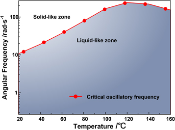
Figure 7. Phase diagram of ESA under oscillatory shear at different temperatures. Loading conditions: oscillatory strain amplitude is set to 0.2%; angular frequency ranges from 0.1 rad/s to 200 rad/s.
Download figure:
Standard image High-resolution imageAs shown in figure 7, as the temperature increases, the critical frequency (the solid red dots in figure 7) of the phase transition increases gradually up to 120 °C and then decreases slightly. At higher temperatures, the polymer chains are more active and more energy is dissipated at the same frequency. On the other hand, ESA is frequency-sensitive (figure 3), the polymer chains are restricted at a higher frequency, and more energy is stored at the same temperature. In other words, temperature and frequency play opposite roles in the dynamic viscoelastic properties of ESA, which is consistent with the experimental data (figure 7). This phase diagram is valuable for engineering applications for choosing suitable or desired loading conditions. For example, if the loading conditions (in this case, we mean the oscillatory frequency and temperature) fall into the liquid-like zone (blue zone) of figure 7, the ESA dissipates more input energy. If more input energy is need to be stored, the loading conditions should be maintained within the solid-like zone (white zone).
We measured the temperature-dependent dynamic viscoelastic properties of ESA at a fixed oscillatory frequency. As shown in figure 8, G' decreases initially with increasing temperature but then clearly increases when the temperature exceeds 140 °C. The largest reduction of G' induced by temperature (in the range of 20 °C∼140 °C) is 104.58, indicating that adjusting the temperature is another method to change the modulus of ESA. The change of modulus induced by temperature is equivalent to the rate-dependent viscoelasticity according to the time-temperature superposition principle (TTSP).

Figure 8. The storage modulus, loss modulus and loss factor of ESA under oscillatory shear at different temperatures. Loading condition: oscillatory strain amplitude is set to 0.2%, angular frequency is set to 10 rad/s.
Download figure:
Standard image High-resolution imageThe temperature-dependent tanδ is calculated based on the relationship of tanδ = G''/G [29]. When the temperature is higher than 24 °C, ESA behaves in a liquid-like state (tanδ > 1), as shown in figure 8. Furthermore, we observe an distinct peak in the tanδ-temperature curve of ESA under oscillatory shear at around 130 °C. Correspondingly, G' and G'' increase when the temperature exceeds to 130 °C and decrease when the temperature is less than 130 °C. No endothermic or exothermic peak is observed in the DSC measurements (figure 9(a)) within the temperature range of −50∼200 °C, indicating that ESA is non-crystalline; thus, TTSP can feasibly be performed. The TG measurements (figure 9(b)) indicate that no degradation takes place in the tested region. Moreover, the results shown in figure 8 are reproducible for the same sample, indicating that the peak is not caused by an irreversible chemical reaction and that the reversible strain rate-hardening behavior is primarily due to reversible breaking and recombining of B-O dative bonds [23]. The storage modulus decreases with increasing temperature because the molecules of the polymer move more easily under high temperatures. When the temperature exceeds a critical value (130 °C in this instance), the configuration of the molecular chains changes and the configuration entropy also increases. A higher configuration entropy induces polymers with a higher elastic modulus [40]. When the temperature exceeds 130 °C, the increment in elastic modulus induced by the configuration entropy exceeds the reduction in elastic modulus induced by temperature; thus we observe an increase of storage modulus and a corresponding decrease of tanδ.

Figure 9. DSC (a) and TGA (b) plots of ESA.
Download figure:
Standard image High-resolution image
4. Conclusions
Dynamic mechanical analysis (DMA) under oscillatory shear is a useful experimental method to study the rate-dependent effect of IHPs. However, due to limitation in current experimental equipment, the rate-dependent viscoelasticity cannot be fully reflected experimentally. To address this issue, we defined a characterization parameter (G+∞/G0) based on Havriliak-Negami (H–N) model, which does not depend on the frequency range. Furthermore, we explored the influence of temperature on the rate-dependent effect and verified the accuracy of the H–N model using the time-temperature superposition principle (TTSP). We concluded that G+∞/G0 provides a better description of the intrinsic viscoelastic properties of ESA than the increment of storage modulus within a specific frequency range. Our method provides an index to quantitatively evaluate the rate-dependent effect of an impact-hardening polymer (in this case, ESA) and is also suitable for any soft viscoelastic material. However, it is need to note that the modulus at very low frequency (i.e. G0) is obtained by extrapolation approach and is very difficult to be verified by experiment. If we choose the same optimization conditions, the comparison of G+∞/G0 for different samples is still valuable. To establish the true constitutive relation of IHPs is the ultimate solution to quantitatively describe the real strain rate-dependent effect. But before this, our method is helpful for deep understanding of the impact hardening mechanism.
We found that except for the viscoelasticity, the phase transition points (i.e., the critical angular frequency at which the storage modulus is equal to the loss modulus, or when tanδ = 1) are also closely related to the oscillatory frequency and temperature. Moreover, we observed that oscillatory frequency and temperature play opposing roles in the phase transition, i.e., the ESA changes from a liquid-like (tanδ > 1) state to a solid-like (tanδ < 1) state at high oscillatory frequency but lower temperatures. We believe that the rate-dependent viscoelasticity model and the phase diagram will be valuable for engineers when choosing the suitable loading conditions for vibration attenuation or impact resistance of newly designed devices.
Acknowledgments
This work was supported by funding from King Abdullah University of Science and Technology (KAUST), and the National Natural Science Foundation of China (Grant Nos. 11502256, 11902309, 11602242). We thank Luyao Yan and Xueyong Liu from Shenzhen Innovation Advanced Materials Co. Ltd for their kind support for the ESA sample and beneficial discussions.