Combined Generative Adversarial Network and Fuzzy C-Means Clustering for Multi-Class Voice Disorder Detection with an Imbalanced Dataset

Abstract

The world has witnessed the success of artificial intelligence deployment for smart healthcare applications. Various studies have suggested that the prevalence of voice disorders in the general population is greater than 10%. An automatic diagnosis for voice disorders via machine learning algorithms is desired to reduce the cost and time needed for examination by doctors and speech-language pathologists. In this paper, a conditional generative adversarial network (CGAN) and improved fuzzy c-means clustering (IFCM) algorithm called CGAN-IFCM is proposed for the multi-class voice disorder detection of three common types of voice disorders. Existing benchmark datasets for voice disorders, the Saarbruecken Voice Database (SVD) and the Voice ICar fEDerico II Database (VOICED), use imbalanced classes. A generative adversarial network offers synthetic data to reduce bias in the detection model. Improved fuzzy c-means clustering considers the relationship between adjacent data points in the fuzzy membership function. To explain the necessity of CGAN and IFCM, a comparison is made between the algorithm with CGAN and that without CGAN. Moreover, the performance is compared between IFCM and traditional fuzzy c-means clustering. Lastly, the proposed CGAN-IFCM outperforms existing models in its true negative rate and true positive rate by 9.9–12.9% and 9.1–44.8%, respectively.

1. Introduction and Literature Review

Voices are crucial for human beings. We communicate with others and express our emotions and ideas through our voices. Throughout our entire lives, we may witness those that have voice disorders, which include abnormalities in quality, tone, volume, and pitch. Voice professionals, whose jobs are strongly related to vocal load and/or voice quality, are highly influenced by voice disorders [1]. Examples include (i) teachers, who require a high vocal load and a medium quality; (ii) television presenters, who require a medium vocal load and a high quality; and (iii) actors, who require a high standard in both vocal load and quality. A healthy voice that fulfills one’s professional needs is important to ensure the best performance.

Various epidemiological studies have suggested a high prevalence of voice disorders. In [2], a prevalence rate of 21% was observed in a sample size of about 4800 people. Another study [3] was conducted in Sweden, in which 16.9% of 114,538 people had voice disorders. Attention was likewise drawn to primary and secondary education teachers in Finland: 54% of 1198 teachers in Finland were found to suffer from voice disorders [4]. Voice disorder sufferers are expected to consult Otorhinolaryngologists and speech therapists for diagnosis and medical treatment to support their rapid recovery. However, research has shown that only a small percentage of total sufferers seek professional advice. Only 5.9% (78 participants) sought professional advice when they suffered from voice disorders [5]. Another survey [6] showed that 22.5% (56 teachers) consulted medical advice to solve their voice disorders. Many of the subjects claimed that they did not recognize they were suffering from voice disorders. Indeed, confirming a voice disorder requires medical knowledge.

Due to the high prevalence and low consultation rate of the population with voice disorders, it is desirable to have an automatic voice disorder detection algorithm with voice inputs that can give an instant diagnosis of a voice disorder, as well as its type. Such algorithms could be integrated into mobile health applications, as demonstrated in related works [7,8].

In Section 1.1, the performance of existing works on voice disorder detection is summarized. The limitations of existing works are explained in Section 1.2, which forms the rationale of the proposed work in addressing these limitations. This is followed by the key contributions of this paper in Section 1.3.

1.1. Literature Review

In recent years, various machine learning algorithms have been proposed and evaluated for the detection of voice disorders. It is worth noting that some previous works [9,10,11] tested their algorithms using the Massachusetts Eye and Ear Infirmary voice and speech lab (MEEI) database, which are not discussed in this paper because the MEEI database is commercialized and not publicly available. Further, it is inconsistent and features varying recording conditions for pathological and healthy subjects.

Instead, this paper focuses on two publicly available databases: the Saarbruechen Voice Database (SVD) [12,13,14,15,16] and Voice ICar fEDerico II (VOICED) [16,17,18]. The following is a summary of existing approaches applied to the SVD. A hybrid support vector machine (SVM) and Gaussian mixture models (GMM) were proposed and evaluated in [12]. This method achieved an accuracy, sensitivity, and specificity of 0.965, 0.94, and 0.99, respectively. Six methods, including a sequential minimum optimization (SMO)-based SVM, decision tree, Bayesian classification, logistic model tree, k-nearest neighbor, and entropy-based method, were evaluated in [13]. The SMO based SVM yielded the best performance in accuracy (0.858), sensitivity (0.876), and specificity (0.839). Guedes et al. [14] proposed two approaches, long short-term memory (LSTM) and convolutional neural network (CNN), for differentiation between healthy and dysphonic candidates, healthy and laryngitic candidates, and healthy and paralyzed candidates. The achieved precision values were 0.66, 0.67, and 0.78, respectively. SVM was applied with zero frequency filtering and quasi-closed phase glottal inverse filtering methods for the detection of voice disorders in [15]. Based on the performance evaluation, the applied method achieved an accuracy, sensitivity, and specificity of 0.76, 0.72, and 0.78, respectively. A threshold-based detection method with a newly defined dysphonia detection index was proposed in [16]. The accuracy, sensitivity, and specificity were 0.798, 0.706, and 0.902, respectively.

The work in [16] also applied VOICED, showing degraded performance in the accuracy, sensitivity, and specificity (of 0.5, 0.458, and 0.643, respectively). Researchers adopted K nearest neighbor (KNN) as a model for the detection of voice disorders [17]. This method achieved an accuracy of 0.933 and outperformed the other algorithms (random forest (0.874) and extra trees (0.863)). In [18], boosted tree, SVM, decision tree, naïve based classifier, and KNN were evaluated; the pairs of sensitivity and specificity were (0.829, 0.862), (0.79, 0.279), (0.779,0.844), (0.857,0.644), and (0.774,0.334), respectively. As the VOICED database was published in 2018 (compared with SVR, which was published in 1997), the research publications that consider the VOICED dataset are fewer than those using SVR.

1.2. Research Gaps and Motivation

Existing works have applied various algorithms for voice disorder detection [12,13,14,15,16,17,18]. However, further research and exploration are necessary to address the following limitations in existing works.

• Some existing works [12,16,17] did not apply cross-validation during their performance evaluation of the algorithms. The first concern is that one may pick up a biased training dataset to train the detection model, which takes advantages of this bias by yielding high accuracy. Secondly, not all the data were evaluated, which may affect the fine tuning of the model and the robustness of its applicability in real-world scenarios.
• There is room for improvement in the accuracy, sensitivity, and specificity of voice disorder detection models [13,14,15,16,18]. Particularly in smart healthcare applications, the performance of the machine learning model has high expectations, as such applications are related to the health status of humans.
• Current works [12,13,14,15,16,17,18] have formulated the voice disorder detection problem as binary detection that only outputs a healthy or pathological result. It is desirable for machine learning algorithms to suggest the actual type of voice disorder to minimize screening time by medical professions.
• Current works [12,13,14,15,16,17,18] have not considered the issues of imbalanced datasets in both SVR and VOICED. This may alter the gap between the sensitivity and specificity of the detection model.

To solve these limitations, this paper adopts the following measures.

• A 10-fold cross validation is adopted for the performance evaluation of the voice disorder detection algorithm.
• The proposed algorithm incorporates a generative adversarial network and fuzzy c-means clustering to improve the performance of the detection model.
• Voice disorder classification is formulated as a multi-class detection problem, thereby allowing the actual type of voice disorder to be suggested.
• A generative adversarial network is proposed to generate new training data, which will reduce the influence of imbalanced datasets and improve the performance of the voice disorder detection model.

1.3. Research Contributions

The contributions of this paper are as follows.

• A conditional generative adversarial network (CGAN) and improved fuzzy c-means clustering (IFCM) algorithm named CGAN-IFCM is proposed to enable the multi-class detection of voice disorders.
• CGAN offers dual benefits, not only reducing the influence of imbalanced datasets but also generating new training data to improve the performance of the voice disorder detection model. In this way, the gap between sensitivity and specificity in the detection model can be reduced. The results indicate that the proposed CGAN-IFCM outperforms stand-alone IFCM by 10–12.6% and 5.8–16.2% for the true negative rate (TNR) and true positive rate (TPR), respectively.
• IFCM addresses the limitations of existing fuzzy c-means clustering (FCM). IFCM increases performance by introducing interactions between adjacent data points in the fuzzy membership function. The data point and its neighboring data points in feature space will have a high probability to be grouped into the same cluster. The results reveal that the proposed CGAN-IFCM improves the TNR and TPR by 7.3–9% and 3.1–12%, respectively.
• Compared with existing works, the proposed CGAN-IFCM improves the TNR and TPR by 9.9–43.5% and 9.1–44.8%, respectively.

2. Materials and Methods

In Section 2, the two publicly available databases (SVD and VOICED) for voice disorder detection are outlined, followed by the proposed CGAN-IFCM algorithm that will be applied to each of the databases.

2.1. Voice Disorders Databases

2.1.1. Saarbruechen Voice Database (SVD)

The SVD was collected in collaboration with the Department of Phoniatrics and Ear, Nose, and Throat (ENT) at the Caritas clinic of St. Theresia in Saarbrücken [19,20]. The data contain recordings of sustained phonations of the vowels, as well as the sentence “Good morning, how are you?” in German. The database includes 869 healthy candidates and 1356 candidates with voice disorders. This can be formulated as a binary detection problem.

For the multi-class detection problem in voice disorders, there are 71 types of pathologies among 1356 candidates. Since most types of pathologies have a small sample size and are aligned with the types of pathologies in VOICED, the multi-class detection problem is formulated as 213 with hyperkinetic dysphonia, 16 with hypokinetic dysphonia, 140 with reflux laryngitis, and 869 healthy.

2.1.2. Voice ICar fEDerico II (VOICED)

VOICED was collected at the faculty of Phoniatrics and Videolaryngoscopy at the Hospital University of Naples Federico II and at the medical room at the Institute of High Performance Computing and Networking [21]. The recordings contain voice signals of the vowel /a/ sustained for five seconds in a quiet room to minimize background noise. Further, VOICED contains information on other attributes, such as smoking status, alcohol consumption, hydration, eating habits, voice handicap index, and reflux symptom index. The database contains 58 healthy candidates and 150 candidates with voice disorders. Thus, the binary detection problem can be formulated.

On the other hand, the multi-class detection problem can be formulated by dividing the voice disorder group into 70 with hyperkinetic dysphonia, 41 with hypokinetic dysphonia, and 39 with reflux laryngitis.

Table 1. Key information on the databases Saarbruecken Voice Database (SVD) and Voice ICar fEDerico II Database (VOICED).

Database	Signal Characteristics	Information Included	Binary Detection Model	Multi-Class Detection Model
SVD [19,20]	16-bit resolution at 50 kHz	Gender, age, and clinical diagnosis	869 healthy candidates and 1356 candidates with voice disorders	869 healthy candidates, 213 with hyperkinetic dysphonia, 16 with hypokinetic dysphonia, and 140 with reflux laryngitis
VOICED [21]	32-bit resolution at 8 kHz	Gender, age, clinical diagnosis, smoking status, alcohol consumption, hydration, eating habits, voice handicap index, and reflux symptom index	58 healthy candidates and 150 candidates with voice disorders	58 healthy candidates, 70 with hyperkinetic dysphonia, 41 with hypokinetic dysphonia, and 39 with reflux laryngitis

summarizes the key information on SVD and VOICED, including the signal characteristics, the information included, and the classes of the binary detection model and multi-class detection model. Both have imbalanced datasets, so CGAN will be applied in this study to generate more training samples for classes with smaller sample sizes.

2.2. Design of the Voice Disorder Detection Model using CGAN-IFCM

In this section, the methodology of CGAN-IFCM is presented. Firstly, this section explains the reasons for using CGAN instead of other types of GAN, along with the details of CGAN. This is followed by the rationale behind the selection of IFCM instead of a traditional FCM as a voice disorder detection model.

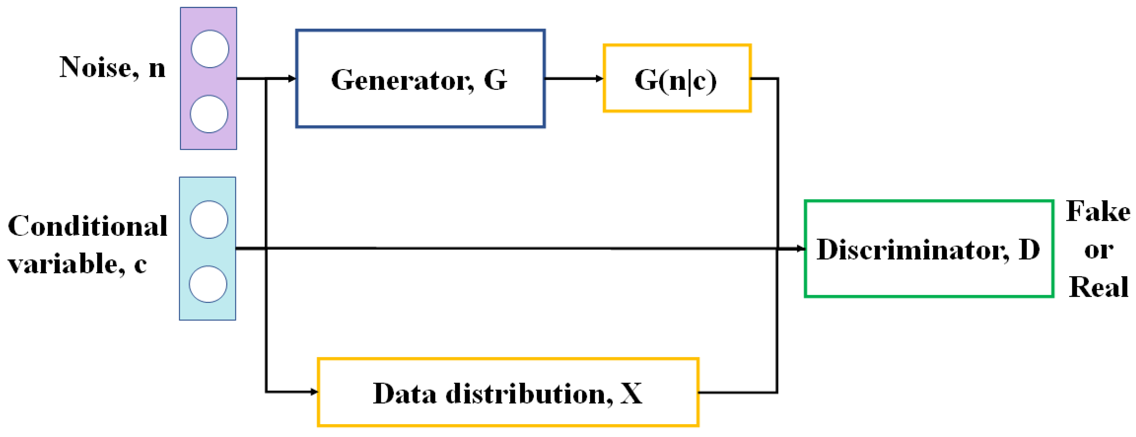
2.2.1. Generation of Additional Training Data Using CGAN

Imbalanced classes were observed in the databases SVD and VOICED. This imbalance causes a significant deviation between the sensitivity and specificity of the voice disorder detection model, particularly in VOICED [16,17,18]. The goal is to increase the number of training samples to balance the classes. A recent state-of-the-art article presented the development and progress of the evolution of GAN [22]. The basic GAN proposal has a key limitation: its noise vector does not have restrictions and may lead to fatal theoretical issues. As a result, different kinds of solutions have been proposed. The following relevant articles have received a large number of citations: auxiliary classifier GAN (ACGAN) [23], CGAN [24], and information maximizing GAN (InfoGAN) [25]. In this paper, CGAN is selected to increase the number of training samples for classes with fewer samples. The first reason is that various types of information (the information included in Table 1) are included in SVD and VOICED. This information is conditional information that fits well with the theory of CGAN. Further, conditional information is introduced in both the generator and discriminator to reduce the aforesaid fatal theoretical issue. Conditional generation is then introduced, in which CGAN is restricted to generate new data for the class of the largest sample size. Therefore, in the binary detection model, the class of candidates with voice disorders is restricted in both SVD and VOICED. For the multi-class detection model, the class of healthy candidates and the class of candidates with hyperkinetic dysphonia are restricted in SVD and VOICED, respectively. To avoid the excessive generation of training data, there is another restriction that involves limiting the number of generated samples of a class to, at most, the original sample size quantity of the corresponding class.

Figure 1 shows the system workflow of CGAN. Given noise vector n and conditional variable c, generator G captures data distribution x, and discriminator D determines whether a sample was from the original dataset or generated dataset. Both G and D are conditioned. Basically, n and c serve as the inputs of G, G serves as the input of G(n|c), and c serves as the input of x. To train a discriminator, D(x; θ_d) gives a single scalar representing the probability that x came from the training data instead of p_data(x). To train the generator distribution p_data(x) using data distribution x, the generator constructs a mapping function from Gaussian noise distribution p_n(n) to the data space as G(n;θ_g). The training of D and G occurs at the same time, where parameters θ_d for D are adjusted to minimize logD(x|c), and parameters θ_g for G are adjusted to minimize log(1 − D(G(n|c))) for the conditional variable c. Mathematically, the objective function is expressed as follows:

$$\underset{G}{\min }\underset{D}{\max }V\left(D,G\right)=E_{x\sim p_{data}\left(x\right)}\left[\log \left(D\left(x|c\right)\right)\right]+E_{x\sim p_n\left(n\right)}\left[\log \left(1-D\left(G\left(n|c\right)\right)\right)\right]$$

(1)

where V(D,G) is the value function.

2.2.2. Voice Disorder Detection Model Using IFCM

As shown in Table 1, the voice disorder detection model can be formulated as a binary detection problem and a multi-class (4-class) detection problem. We selected a multi-class detection model for the illustration in this subsection because it represents the expected application through which the voice disorder detection model could diagnose actual types of voice disorders.

To design the feature vector, there are two typical approaches: (i) follow clinical and expert guidelines; and (ii) if the first approach is not available, a thorough investigation of the proper features should be carried out. For the voice disorder detection problem, we follow the first approach because there is a clinical acoustic analysis technique available for the formal assessment of voice disorders [26,27]. Four voice quality-based parameters are chosen. These qualities are harmonic to the noise ratio (HNR), shimmer, jitter, and fundamental frequency (f₀). Since the estimations of these parameters are a standard approach, and feature extraction is not the focus of this paper, we follow de Krom’s algorithm to measure HRN [28], jitter (as the cycle-to-cycle variation of fundamental frequency) [29], shimmer (as the peak-to-peak amplitude variation in decibels) [29], and f₀ (as the maximal of autocorrelation function) [30].

In the implementation and performance evaluation, we adopt k-fold cross-validation, with k = 10 as the typical order [31,32]. We define N_i as the total number of samples in class 1, where N₁, N₂, N₃, and N₄ correspond to healthy candidates, those with hyperkinetic dysphonia, those with hypokinetic dysphonia, and those with reflux laryngitis, respectively. The feature vector is X_p = {HRN_p, jitter_p, shimmer_p, f_0,p} for p = [1, 0.9(N₁ + N₂ + N₃ + N₄)], where 0.9(N₁ + N₂ + N₃ + N₄) is equivalent to 90% of the training dataset.

In general, the FCM problem is defined to minimize the objective function [33]. Intuitively, in each cluster, the data points should be close to the cluster center. Therefore, the objective is defined as a minimization of the intra-cluster variance, which is equivalent to a maximization of intra-cluster similarities. The less the variance, the greater the similarities among the data points. For example, a variance of zero results in maximal similarity:

$$F_{FCM}={\displaystyle \sum _{p=1}^{\left(0.9\right)\left(N_1+N_2+N_3+N_4\right)}\sum _{c=1}^{N_c}}{u}_{pc}^m{\left|\left|X_p-v_c\right|\right|}^2,1\le m\le \infty$$

(2)

$$\mathrm{s}.\mathrm{t}.{\sum }_{c=1}^{N_c}{u}_{pc}=1$$

(3)

where N_c is the optimally designed total number of clusters using the multiobjective genetic algorithm (MOGA), u_pc is the degree of membership of X_p in the cth cluster, v_c is the cluster center of the cth cluster, and m controls the fuzziness of the resulting partition. The value m = 2 is common and is selected according to [33].

Taking the partial derivative, we have two iterative solutions, v_c and u_pc, given by

$$v_c=\frac{{\sum }_{p=1}^{\left(0.9\right)\left(N_1+N_2+N_3+N_4\right)}{u}_{pc}^m·X_p}{{\sum }_{p=1}^{\left(0.9\right)\left(N_1+N_2+N_3+N_4\right)}{u}_{pc}^m}$$

(4)

$$u_{pc}=\frac{{\sum }_{p=1}^{N_c}{\left|\left|X_p-v_p\right|\right|}^{\frac{2}{m-1}}}{|\left|X_p-v_c\right|{|}^{\frac{2}{m-1}}}.$$

(5)

Nonetheless, the existing FCM algorithm [33] does not include the relationship between X_p and its neighbor X_p, which limits its performance in clustering problems. Feature vector X_p is indeed strongly correlated (sharing similar characteristic) to its neighbor X_p due to the nature of characteristics in the feature space. These X_p values have a high probability to be grouped into the same cluster. As a result, the rationale of the proposed work is to introduce the interaction between X_p and its neighbor X_p into the fuzzy membership function.

A new degree of membership is proposed as follows:

$$u_{neighbor,pc}=\frac{C_{pc}·{\sum }_{p=1}^{N_c}{\left|\left|X_p-v_p\right|\right|}^{\frac{2}{m-1}}}{|\left|X_p-v_c\right|{|}^{\frac{2}{m-1}}}$$

(6)

$$C_{pc}=\frac{{\sum }_{j\in SN\left(X_p\right)}{u}_{jc}}{N_n}$$

(7)

where C_pc is a conditional variable related to the level of participation of X_p in the cth cluster, SN(X_p) is the square neighborhood centered at X_p, and N_c is the number of feature vectors in the neighborhood.

The joined degree of membership between u_pc and u_neighbor,pc is defined as follows:

$$u_{VDC,pc}=\frac{{(u_{neighbor,pc})}^{{\omega }_n}{(u_{pc})}^{{\omega }_0}}{{\sum }_{q=1}^{N_n}\left(u_{neighbor,pq}\right)\left(u_{pq}\right)}$$

(8)

$$v_{VDC,c}=\frac{{\sum }_{p=1}^{\left(0.9\right)\left(N_1+N_2+N_3+N_4\right)}{u}_{VDC,pc}^m·X_p}{{\sum }_{p=1}^{\left(0.9\right)\left(N_1+N_2+N_3+N_4\right)}{u}_{VDC,pc}^m}$$

(9)

where ${\omega }_n$ and ${\omega }_0$ are the control weighting factors of the importance between u_neighbor,pc and u_pc. These are optimally designed via MOGA, which benefits the convergence of the model training. There are numerous combinations of ${\omega }_n$ and ${\omega }_0$ which may yield different $u_{VDC,pc}$ and $v_{VDC,c}$ values. Searching for the optimal ${\omega }_n$ and ${\omega }_0$ requires considerable computing power. Alternatively, a tradeoff is sought between the convergence of model training and computing power while maintaining favorable performance.

The multiobjective optimization problem consists of four objectives, given by

$$\{\begin{array}{cc}MAX& F_1=C{H}_{index}\\ \begin{array}{c}MIN\\ \begin{array}{c}MAX\\ MAX\end{array}\end{array}& \begin{array}{c}{F}_2=\left|\left|U_{VDC}{}^{\left(b+1\right)}-U_{VDC}{}^{\left(b\right)}\right|\right|\\ \begin{array}{c}{F}_3=Specificity=TNR\\ F_4=Sensitivity=TPR\end{array}\end{array}\end{array}$$

(10)

where CH_index is the Calinski–Harabasz (CH) index, which is important to determine the number of clusters [34]. CH_index evaluates the cluster validity based on the sum of the square between the cluster and the sum of the square within the cluster. Varying the number of clusters N_c yields distinct values of CH_index: The higher the CH_index is, the better the solution. In addition, U_VDC = (u_VDC,pc)_{(N1+N2+N3+N4)∗(Nc)} is the fuzzy membership matrix, TNR is the true negative rate (equivalent to specificity), and TPR is the true positive rate (equivalent to sensitivity) of the voice disorder detection model. CH_index, TNR, and TPR are given by

$$C{H}_{index}=\frac{S{S}_{BC}/\left(N_c-1\right)}{S{S}_{WC}\left(\left(0.9\right)\left(N_1+N_2+N_3+N_4\right)-N_c\right)}$$

(11)

$$Specificity=TNR=\frac{TN}{TN+FP}$$

(12)

$$Sensitivity=TPR=\frac{TP}{TP+FN}$$

(13)

where SS_BC is the sum of the square between clusters, N_c is the number of clusters, SS_WC is the sum of the square within the cluster. The larger the SS_BC is, the higher the degree of dispersion between the clusters becomes. The smaller the SS_WC is, the closer the relationship in the cluster. In addition, TN is the true negative, FP is the false positive, TP is the true positive, and FN is the false negative of the testing samples.

The proposed MOGA-IFCM algorithm is then applied to solve the multiobjective optimization problem in Equation (10) [35,36]. Generally, solving a multiobjective optimization problem has an overall run time complexity of O(GMN²), where G, M, and N are the number of generations, number of objectives, and population size, respectively. We adopted a hyper-grid scheme [37,38] to reduce the time complexity. The calculation of individual sharing functions is restricted only to individuals in neighboring cells. Each cell contains a few individuals. The overall time complexity is thus reduced to O(GMN).

Evolutionary algorithms (for instance, the genetic algorithm) tend to converge to a single solution as the diversity of the population diminishes [39]. This phenomenon is called genetic drift. The technique for maintaining a stable sub-population of diverse individuals according to the distance between individuals is called the niching technique. An individual’s niche count is defined as the sum of the sharing function sf (i.e., ${\sum }_{j=1}^{n}sf\left(d\left(i,j\right)\right)$), whose values lies between itself and every individual in the population. We can define sf as a function of distance d(i,j) between the two population elements, as follows [40,41]:

$$sf\left(d\right)=\{\begin{array}{cc}1-{\left(\frac{d\left(i,j\right)}{{\sigma }_{dis}}\right)}^{\alpha }& ifd<{\sigma }_{dis}\\ 0& otherwise\end{array}$$

(14)

where ${\sigma }_{dis}$ is the threshold for dissimilarity, and $\alpha =1$ is a constant for regulating the shape of the sharing function.

The optimal tradeoff solutions are thus found. Pseudo code of the algorithm can be found in Algorithm 1.

Algorithm 1$TrainSVC({\left\{X_p\right\}}_{train},b)$

Input: {Xp}train, m = 2

Output: Model

1. Generation count g = 1;

2. Initialize population;

3. Evaluate the individuals with the fitness functions (F1, F2, F3, and F4);

4. Rank the fitness values of individuals based on step 3;

5. Calculate the Niche count;

while generations <= max_generation do

6. Select two parents from the population;

7. Create offspring using Roulette wheel selection (RWS), crossover, and mutation;

8. Train a MOGA-based IFCM model for each individual;

9. Evaluate the offspring with the fitness functions (F1, F2, F3, and F4);

10. Rank the offspring by their fitness values according to step 9

11. Calculate the Niche count;

12. Decide the new population based on the offspring;

13. g = g + 1;

End while

Model←Pareto solutions

3. Analysis and Results of CGAN-IFCM

The effectiveness of the proposed CGAN-IFCM is analyzed in four parts: (i) the performance of the proposed CGAN-IFCM; (ii) the necessity of using CGAN by comparing the performance of the detection models using CGAN-IFCM and IFCM; (iii) the necessity of using IFCM by comparing the performance of the detection models using CGAN-IFCM and CGAN-FCM; (iv) comparing CGAN-IFCM with two typical data generation methods (synthetic minority oversampling technique (SMOTE) and cost-sensitive learning (CSL)); (v) comparing the performance between CGAN-IFCM and existing methods. As previously noted, 10-fold cross-validation was adopted for performance evaluation, for which the value of 10 has been widely adopted in the literature [31,32].

3.1. Performance Evaluation of CGAN-IFCM

As shown in Table 1, there are four cases of formulations: (i) the binary detection model using the SVD database; (ii) the binary detection model using the VOICED database; (iii) the multi-class detection model using the SVD database; (iv) the multi-class detection model using the VOICED database. Section 3.1 will present and analyze the results of CGAN-IFCM in all these cases.

3.1.1. Binary Detection Model using CGAN-IFCM

Consider that the proposed CGAN-IFCM, the number of clusters N_c, and conditioning variables ${\omega }_n$ and ${\omega }_0$ highly influence the joined degree of membership $u_{VDC,pc}$ and cluster center $v_{VDC,c}$ and thus correlate to the performance (TNR and TPR) of the detection model.

The evaluation is first performed on the binary detection model using CGAN-IFCM with the SVD database.

Table 2. Performance evaluation of the binary detection model using CGAN-improved fuzzy c-means clustering (IFCM) with varying N_c, ${\omega }_n$, and ${\omega }_0$ values using the SVD database. (a) Fixed ${\omega }_n=1.8$. (b) Fixed ${\omega }_n=1.9$. (c) Fixed ${\omega }_n=2.0$. (d) Fixed ${\omega }_n=2.1$. (e) Fixed ${\omega }_n=2.2$.

Control Weighting Factors		TNR (%)/TPR (%) with Varying ${\mathit{N}}_{\mathit{c}}$
${\mathit{\omega }}_{\mathit{n}}$	${\mathit{\omega }}_{\mathbf{0}}$	3	4	5	6	7	8	9	10
2	2	90.9/90.2	93.6/95.2	91.3/93.6	88.2/89.3	85.3/86.3	82.6/83.3	77.7/78.8	74.3/73.8
	2.1	87.8/88.5	89.7/90.2	87.3/88.2	85.4/87.0	82.9/82.1	80.1/80.8	75.6/74.5	72.3/71.7
	2.2	86.1/85.8	87.7/86.9	86.8/85.0	84.2/84.5	81.3/81.5	78.8/78.0	74.1/73.2	70.8/71.8
	2.3	84.9/84.6	85.8/86.1	84.2/83.5	83.3/82.7	80.8/81.2	77.1/77.3	73.8/72.5	69.8/70.2
	2.4	82.5/82.1	83.9/84.1	83.1/82.7	82.4/81.8	80.4/79.7	75.5/76.3	71.8/73.1	68.6/69.1
2.1	2	91.6/91.8	94.3/95.1	92.8/92.1	89.7/90.6	86.8/85.6	84.2/84.8	78.3/79.6	74.3/73.8
	2.1	90.3/91.2	93.7/92.8	92.0/91.7	90.1/89.2	86.3/85.7	83.5/82.9	77.3/77.8	73.6/73.1
	2.2	89.1/89.4	91.6/92.0	90.7/91.1	89.5/88.8	85.3/84.6	82.4/82.1	76.5/76.9	72.1/72.9
	2.3	87.6/87.0	90.2/90.5	88.9/87.7	87.4/85.8	84.7/84.0	81.8/81.1	75.9/75.2	71.4/72.0
	2.4	85.8/85.1	88.4/88.9	86.5/86.1	85.4/85.1	84.1/84.5	80.6/80.0	73.6/73.5	72.1/71.2
2.2	2	91.9/92.3	94.6/95.4	93.2/92.3	89.9/91.0	87.5/85.9	84.6/85.2	78.7/78.2	74.8/74.2
	2.1	90.6/91.4	94.1/93.2	92.4/92.2	90.5/89.6	86.7/86.2	84.0/83.3	77.7/78.1	73.9/73.3
	2.2	89.6/89.9	91.8/92.3	91.0/91.3	89.8/88.9	85.7/84.9	82.8/82.4	76.9/77.2	72.4/73.5
	2.3	87.8/87.3	90.4/90.6	89.2/87.9	87.8/87.5	85.2/84.5	82.4/81.3	76.3/75.5	71.7/72.3
	2.4	86.0/85.5	88.8/89.2	86.8/86.3	85.8/86.3	84.6/84.8	80.9/80.3	74.0/73.9	72.5/71.4
2.3	2	91.2/92.3	94.3/95.3	93.1/91.9	89.8/90.6	86.9/85.7	84.6/84.6	77.6/77.2	73.0/73.5
	2.1	90.1/90.4	93.8/92.9	91.3/91.6	90.0/89.1	85.8/85.3	83.3/82.9	77.3/77.1	72.8/72.3
	2.2	87.8/88.2	90.2/91.1	90.3/89.9	88.7/88.1	84.9/84.1	82.2/81.8	76.4/76.8	71.1/70.9
	2.3	86.5/87.1	88.9/89.5	89.6/88.8	87.4/87.0	84.2/83.6	81.2/80.5	75.6/76.1	70.9/70.3
	2.4	85.4/86.3	87.5/88.2	88.2/87.3	86.8/86.2	83.6/82.8	80.3/79.7	74.2/74.5	69.5/69.8
2.4	2	90.4/91.8	93.1/94.2	92.5/91.3	88.6/89.5	86.1/84.9	83.5/83.9	76.9/76.3	72.1/72.3
	2.1	89.2/89.1	92.8/92.4	90.7/91.1	89.2/88.4	85.2/84.7	82.7/82.2	76.7/76.2	72.0/71.5
	2.2	87.5/87.9	89.7/90.8	89.6/89.2	88.2/87.4	84.4/82.6	81.7/81.1	75.8/76.0	70.4/70.1
	2.3	85.8/86.3	88.1/88.9	89.0/88.1	86.9/86.3	83.8/83.2	80.4/79.8	75.1/75.7	70.2/69.9
	2.4	84.9/85.8	87.1/87.8	87.5/86.8	86.2/85.8	83.1/82.5	80.0/79.5	73.7/74.1	69.2/69.5

summarizes the TNR and TPR of the selected scenarios with $N_c=\left[3,10\right]$, ${\omega }_n,{\omega }_0=\left[2,2.4\right]$, with step size of 1 and 0.1, respectively. Key observations can be drawn from this process:

• (${\omega }_n=2$): The membership $u_{VDC,pc}$ is more dominated by ${\omega }_0=2$. Therefore, ${\omega }_0$ increases as the TNR and TPR decrease.
• (${\omega }_n=\left[2.1,2.4\right]$): The highest TNR and TPR are obtained at ${\omega }_0=2$. This can be explained by the case that if ${\omega }_n>{\omega }_0$. Recall that X_p and its neighbor X_p share similar characteristics and tend to group under the same $v_{VDC,c}$. However, when ${\omega }_n\le {\omega }_0$, both TNR and TPR decrease.
• The performance of CGAN-IFCM is better when $N_c=\left[3,5\right]$ compared to $N_c=\left[6,10\right]$ and deteriorates significantly when $N_c>5$, as some clusters could be redundant and lead to errors in voice disorder detection.

As a result, the voice disorder detection model achieves higher accuracy when ${\omega }_n>{\omega }_0$, which reveals the effectiveness and necessity of the membership function u_neighbor,pc and weighting factor ${\omega }_n$. On the other hand, when ${\omega }_n\le {\omega }_o$, $u_{VDC,pc}$ tends to be dominated by ${\omega }_0$, which is close to the performance of existing FCM algorithms.

Next, we focus on the binary detection model with the VOICED database. Similarly,

Table 3. Performance evaluation of the binary detection model using CGAN-IFCM with varying N_c, ${\omega }_n$, and ${\omega }_0$ values with the VOICED database. (a) Fixed ${\omega }_n=1.8$. (b) Fixed ${\omega }_n=1.9$. (c) Fixed ${\omega }_n=2.0$. (d) Fixed ${\omega }_n=2.1$. (e) Fixed ${\omega }_n=2.2$.

Control Weighting Factors		TNR (%)/TPR (%) with Varying ${\mathit{N}}_{\mathit{c}}$
${\mathit{\omega }}_{\mathit{n}}$	${\mathit{\omega }}_{\mathbf{0}}$	3	4	5	6	7	8	9	10
2	2	83.7/87.9	88.3/92.1	87.5/90.8	84.6/87.9	81.6/84.7	79.8/82.3	73.7/77.3	70.2/73.0
	2.1	82.1/86.0	86.8/89.6	85.9/88.8	83.7/86.9	79.7/82.4	77.5/80.0	73.5/75.9	69.8/72.1
	2.2	81.3/85.2	85.1/87.5	83.1/85.5	82.1/85.6	78.9/81.9	76.4/78.9	71.5/74.2	68.6/71.5
	2.3	80.2/84.8	83.3/86.6	81.8/84.2	81.0/83.9	77.5/81.4	74.9/77.8	70.6/73.2	67.3/70.8
	2.4	79.7/83.5	82.1/85.3	80.2/83.5	80.3/82.6	76.9/80.3	73.8/77.2	69.7/72.4	66.8/70.1
2.1	2	87.0/90.4	90.9/93.6	89.7/92.3	86.3/90.8	83.2/86.5	81.4/84.5	76.6/80.3	71.5/74.9
	2.1	86.2/89.7	89.6/92.2	88.3/91.5	85.6/89.3	81.8/85.5	80.1/83.5	75.8/78.5	70.1/73.8
	2.2	85.5/88.8	88.7/91.5	87.4/90.9	84.9/88.5	80.4/84.8	80.0/83.1	74.2/77.4	68.8/72.8
	2.3	84.7/87.3	87.4/90.9	85.3/88.6	83.8/87.4	79.6/83.8	78.7/82.0	73.3/76.8	67.9/71.7
	2.4	82.8/85.7	85.3/89.2	84.2/87.2	82.7/86.3	78.6/82.9	77.3/80.5	71.0/74.2	67.3/71.1
2.2	2	88.2/91.4	91.1/93.8	89.9/92.5	86.7/91.6	84.0/87.4	82.1/86.1	77.6/80.3	72.6/75.6
	2.1	87.2/90.6	90.2/93.1	89.3/92.1	86.9/90.3	83.0/86.6	81.7/84.0	75.1/79.2	71.5/74.2
	2.2	86.1/89.4	89.2/92.0	88.1/91.5	85.6/89.4	82.4/85.3	81.4/83.7	74.5/78.6	69.3/73.3
	2.3	85.2/88.1	88.2/91.3	85.7/88.7	84.9/88.1	81.8/84.7	80.1/83.2	73.6/76.3	68.9/72.1
	2.4	83.1/86.7	86.4/90.6	83.8/87.9	82.8/87.2	80.6/83.5	78.7/81.9	72.3/75.6	68.6/71.8
2.3	2	89.2/92.3	91.5/94.3	90.6/93.4	87.8/92.0	85.3/88.6	82.5/86.8	78.0/81.6	72.9/76.3
	2.1	87.8/90.9	88.6/93.6	88.5/92.5	87.4/90.5	83.6/87.7	81.9/84.6	75.5/79.8	72.1/74.7
	2.2	86.6/90.1	88.4/91.5	88.2/90.3	86.5/89.8	83.4/86.3	81.6/82.5	74.9/79.3	70.2/72.5
	2.3	85.5/88.5	88.4/91.1	86.3/89.4	85.7/88.4	82.5/85.8	80.2/83.1	74.2/76.8	69.6/72.0
	2.4	84.1/87.3	87.1/90.9	85.5/88.8	84.5/87.8	81.1/84.3	79.8/80.5	73.2/76.2	69.1/71.2
2.4	2	87.1/90.4	88.5/92.3	86.7/89.9	85.2/88.0	83.8/86.6	81.8/85.3	76.5/79.8	72.5/75.8
	2.1	85.8/88.5	87.4/90.7	86.2/89.3	84.6/87.1	83.0/85.9	79.7/83.8	75.3/78.9	71.7/74.9
	2.2	85.0/87.5	86.5/89.2	85.3/88.5	84.1/87.0	82.2/85.3	78.5/82.9	74.3/77.0	70.4/73.6
	2.3	84.2/87.2	85.5/88.6	84.7/87.5	83.6/86.6	81.7/84.3	79.8/80.3	73.7/76.3	69.7/72.4
	2.4	83.4/86.5	84.7/87.3	83.7/86.6	82.7/85.5	82.0/83.7	76.3/79.3	72.4/75.6	68.5/70.7

summarizes the TNR and TPR of the selected scenarios with $N_c=\left[3,10\right]$ and ${\omega }_n,{\omega }_0=\left[2,2.4\right],$ with step sizes of 1 and 0.1, respectively. Besides following the same observations shown in Table 2, there are two extra observations.

• The detection model is dominated by a class of candidates with voice disorders because the number of samples of voice disorders remains larger than the number of samples of healthy candidates after the adoption of CGAN. In other words, as shown in Table 3, there is a notable gap (on average, 3.94% versus 0.79%, as shown in Table 2) between TNR and TPR, where TPR is higher than TNR.
• The overall accuracy of the binary detection model with the VOICED database is less than that of the SVD database. This could be explained in two ways: the imbalanced dataset in SVD and the number of samples in SVD, which is 10 times that in VOICED.

3.1.2. Multi-Class Detection Model using CGAN-IFCM

For the construction of the multi-class detection model, the problem is extended to determining the exact type of voice disorders from among four possibilities: healthy, hyperkinetic dysphonia, hypokinetic dysphonia, and reflux laryngitis. First, the SVD database is considered.

Table 4. Performance evaluation of the multi-class detection model using CGAN-IFCM while varying N_c, ${\omega }_n$, and ${\omega }_0$ with the SVD database. (a) Fixed ${\omega }_n=1.8$. (b) Fixed ${\omega }_n=1.9$. (c) Fixed ${\omega }_n=2.0$. (d) Fixed ${\omega }_n=2.1$. (e) Fixed ${\omega }_n=2.2$.

Control Weighting Factors		TNR (%)/TPR (%) with Varying ${\mathit{N}}_{\mathit{c}}$
${\mathit{\omega }}_{\mathit{n}}$	${\mathit{\omega }}_{\mathbf{0}}$	3	4	5	6	7	8	9	10
2	2	83.2/79.6	84.3/80.0	85.6/80.8	86.1/81.9	90.3/86.3	89.2/85.1	86.0/83.6	83.8/79.5
	2.1	82.2/78.7	83.0/79.1	83.5/79.6	84.4/80.3	87.8/84.6	87.0/83.8	85.4/82.5	81.2/77.7
	2.2	81.2/77.0	82.0/77.9	82.6/78.7	83.4/79.8	85.7/83.6	83.6/81.4	83.8/80.2	80.1/76.8
	2.3	79.8/75.9	80.6/76.8	81.6/77.9	82.2/78.4	84.8/81.8	82.1/80.1	82.3/79.4	79.7/75.3
	2.4	78.9/75.5	80.0/75.7	80.3/76.5	81.3/77.5	83.7/80.6	81.7/78.6	81.1/78.5	78.3/74.3
2.1	2	85.4/80.3	86.2/81.2	87.0/82.3	88.2/84.6	91.2/86.8	89.9/85.5	88.3/84.9	86.1/82.6
	2.1	84.2/79.5	85.4/80.6	86.3/81.4	87.4/83.2	90.3/85.6	89.5/84.7	87.6/83.1	85.3/81.3
	2.2	83.6/78.7	84.3/80.0	85.2/80.3	86.3/82.3	89.5/84.2	88.6/83.6	87.1/82.3	84.4/80.5
	2.3	82.5/77.7	83.2/79.1	84.1/79.7	85.3/81.6	88.8/83.1	87.5/82.6	86.3/81.2	83.2/79.8
	2.4	81.3/76.9	82.4/78.1	83.4/78.7	84.5/80.9	86.3/82.0	84.9/81.3	84.1/80.5	82.3/79.1
2.2	2	86.1/81.8	87.2/82.5	88.2/84.0	89.3/85.6	91.6/87.6	90.3/86.4	88.9/85.3	87.6/84.1
	2.1	85.2/80.5	86.0/81.3	87.1/83.5	88.0/84.2	90.3/86.3	89.6/85.0	87.8/84.1	86.4/83.7
	2.2	84.3/79.6	85.3/80.7	86.3/82.0	87.2/83.6	89.6/85.5	88.8/84.3	86.3/83.2	85.6/82.7
	2.3	83.4/78.7	84.6/79.9	85.6/80.9	86.4/82.8	89.1/84.6	88.5/83.8	85.5/82.6	84.8/81.2
	2.4	81.5/77.9	82.6/79.2	83.3/80.0	83.8/81.8	87.5/83.8	86.8/82.6	85.0/81.3	83.6/80.8
2.3	2	87.6/82.1	88.5/83.4	89.4/85.3	90.6/85.9	92.1/88.5	90.4/86.9	89.7/86.2	88.8/85.3
	2.1	86.3/81.3	87.6/82.8	88.5/84.5	88.8/84.8	91.2/87.3	90.0/85.8	88.7/85.1	87.2/84.6
	2.2	85.4/80.1	86.2/81.3	87.3/83.6	86.3/84.1	90.2/86.6	89.3/85.3	87.2/84.1	86.6/83.5
	2.3	84.6/79.6	85.8/80.5	86.2/81.3	85.3/83.6	89.7/85.3	89.0/84.2	86.0/83.5	85.2/82.6
	2.4	82.5/79.3	83.1/80.5	83.8/81.5	84.3/82.5	88.8/84.3	87.8/83.6	86.3/82.6	83.9/81.2
2.4	2	84.5/80.0	85.8/81.3	87.1/82.6	88.4/83.5	90.2/86.1	87.3/84.8	85.1/83.7	83.6/82.4
	2.1	83.8/79.1	85.0/81.2	86.0/81.4	87.1/82.3	89.6/85.2	86.6/83.1	84.0/82.5	82.3/81.5
	2.2	82.4/78.0	83.5/79.5	84.2/80.3	85.1/81.6	88.2/84.5	85.8/82.2	82.6/81.7	81.0/80.4
	2.3	81.3/77.2	82.4/78.7	83.5/79.6	84.7/80.8	86.8/83.2	84.9/81.6	81.1/80.8	80.1/79.8
	2.4	80.4/76.3	81.5/77.5	82.0/78.5	83.2/79.4	85.6/81.3	83.6/80.3	80.2/78.1	79.6/76.7

presents the TNR and TPR of selected scenarios with $N_c=\left[3,10\right]$, ${\omega }_n,{\omega }_0=\left[2,2.4\right]$, and a step size of 1 and 0.1, respectively. In addition to the first two points stated in Table 2, there are three other observations.

• The performance of CGAN-IFCM is better when $N_c=\left[6,8\right]$ compared to $N_c=\left[3,5\right]$ and $N_c=\left[9,10\right]$. It achieves lower performance when $N_c<6$ and $N_c>8$ as either an insufficient number of clusters or redundant clusters are considered.
• The detection model is dominated by the class of healthy candidates because the number of samples of healthy candidates is far greater than the number of samples of candidates with hyperkinetic dysphonia, hypokinetic dysphonia, or reflux laryngitis after the adoption of CGAN. In Table 4, there difference between TNR and TPR (where TNR is higher than TPR) is further increased (on average, by 4.56% versus 3.94%, as shown in Table 3) between TNR and TPR, where TPR is higher than TNR.
• The overall accuracy of the multi-class detection model is lower than that of the binary-class detection model. Basically, the multi-class detection model is a more complicated problem compared to the binary classifier. Further, the issue of an imbalanced dataset is especially significant given the small sample size of patients with hypokinetic dysphonia (2% of the samples of healthy candidates).

Next, the multi-class detection model is implemented using the VOICED database.

Table 5. Performance evaluation of the multi-class detection model using CGAN-IFCM under varying N_c, ${\omega }_n$, and ${\omega }_0$ values with the VOICED database. (a) Fixed ${\omega }_n=1.8$. (b) Fixed ${\omega }_n=1.9$. (c) Fixed ${\omega }_n=2.0$. (d) Fixed ${\omega }_n=2.1$. (e) Fixed ${\omega }_n=2.2$.

Control Weighting Factors		TNR (%)/TPR (%) with Varying ${\mathit{N}}_{\mathit{c}}$
${\mathit{\omega }}_{\mathit{n}}$	${\mathit{\omega }}_{\mathbf{0}}$	3	4	5	6	7	8	9	10
2	2	81.5/82.1	83.0/82.6	83.4/82.7	84.9/85.3	87.6/87.0	86.2/86.7	84.3/83.1	82.6/81.8
	2.1	80.3/81.4	82.3/81.8	83.0/82.3	83.5/84.1	85.9/86.2	84.5/85.9	83.6/82.1	82.0/80.4
	2.2	79.5/78.7	80.7/80.3	81.5/82.1	82.7/83.5	84.6/84.0	83.2/82.7	83.1/82.6	81.3/79.3
	2.3	77.6/78.0	78.6/78.5	80.2/80.7	81.6/82.3	83.3/82.4	82.5/81.8	81.7/80.7	80.5/78.6
	2.4	77.0/76.8	78.1/77.3	79.6/78.5	80.7/81.2	82.4/81.8	81.2/80.7	80.3/79.6	79.2/77.7
2.1	2	82.5/82.8	84.0/83.1	85.1/84.0	86.3/85.8	88.5/88.0	87.2/86.8	85.8/85.2	83.1/83.3
	2.1	81.4/81.6	83.2/82.2	84.0/83.5	85.7/84.8	86.9/87.1	85.9/86.3	84.5/84.8	82.6/82.2
	2.2	80.8/80.3	82.1/81.6	83.2/82.6	84.0/83.9	85.3/86.0	84.1/85.0	83.6/83.9	82.1/81.5
	2.3	79.3/78.9	81.0/80.4	82.3/81.5	83.6/82.9	84.6/83.9	83.9/83.3	82.1/82.6	81.1/80.5
	2.4	78.1/77.5	79.6/79.0	81.1/80.8	82.3/81.6	83.5/82.6	82.5/82.4	81.0/81.4	80.6/79.6
2.2	2	84.2/83.7	85.3/84.4	86.7/85.9	87.5/86.7	88.7/88.8	87.5/87.1	86.4/86.0	84.9/85.1
	2.1	82.8/82.2	84.5/83.7	85.8/84.9	86.8/85.3	87.6/88.0	87.2/87.2	85.6/85.4	83.8/84.5
	2.2	81.1/80.9	83.2/81.8	84.8/83.5	85.7/84.7	86.3/87.2	86.3/85.9	84.5/84.7	83.1/84.0
	2.3	80.3/80.1	82.5/81.1	83.6/82.8	84.4/83.5	85.7/86.1	84.6/84.3	83.6/83.3	82.3/82.6
	2.4	79.3/78.7	81.2/80.6	82.6/82.1	83.4/82.6	84.8/85.3	83.9/83.5	83.1/82.7	81.6/81.5
2.3	2	85.4/84.9	86.8/85.3	87.8/86.5	88.2/87.8	89.2/89.9	88.1/88.4	87.3/87.6	86.5/85.8
	2.1	84.1/83.7	85.2/84.6	87.0/86.2	87.5/87.2	88.5/88.8	87.4/87.0	86.2/86.3	85.0/84.5
	2.2	83.2/82.6	84.5/83.4	86.1/85.7	87.1/86.5	87.9/88.2	86.1/86.5	85.5/85.2	84.1/83.8
	2.3	82.5/81.4	83.7/82.8	84.6/85.0	85.6/85.2	86.5/87.1	85.3/86.1	84.8/84.1	83.6/82.0
	2.4	81.3/80.5	82.6/81.8	83.5/83.6	84.9/84.4	85.6/86.0	84.5/85.0	83.6/83.9	82.5/81.1
2.4	2	83.2/82.6	84.3/83.7	85.8/84.3	86.5/85.4	87.8/87.2	86.4/85.3	84.3/83.2	83.1/82.5
	2.1	82.5/82.0	83.6/82.8	84.5/83.7	85.8/85.0	86.5/86.1	85.3/84.4	83.1/82.9	82.0/81.3
	2.2	81.2/81.5	82.7/82.3	83.6/82.9	84.6/84.1	85.8/84.5	84.5/83.2	83.7/82.6	81.4/80.8
	2.3	80.4/81.0	81.8/81.5	82.7/82.3	83.9/83.4	85.2/83.6	83.5/82.7	82.5/81.9	80.5/79.3
	2.4	79.6/80.1	80.3/80.8	81.5/81.3	82.6/82.8	84.9/83.3	82.8/81.9	81.7/80.5	79.3/78.5

presents the TNR and TPR of the selected scenarios with $N_c=\left[3,10\right]$, ${\omega }_n,{\omega }_0=\left[2,2.4\right]$, and a step size of 1 and 0.1, respectively. In addition to the first two points stated in Table 2, there are two other observations.

• The performance of CGAN-IFCM is better when $N_c=\left[6,8\right]$ compared to $N_c=\left[3,5\right]$ and $N_c=\left[9,10\right]$. It achieves lower performance when $N_c<6$ and $N_c>8$, as either an insufficient number of clusters or redundant clusters are considered.
• The multi-class detection model is formulated using an equal sample size in each class after the adoption of CGAN. The difference between TNR and TPR is not significant, and there is no bias in TNR, which is either always higher than TPR, or TPR is always higher than TNR.

3.2. Comparison Between CGAN-IFCM and IFCM

IFCM includes the relationship between X_p and its neighbor X_p, which enhances the performance of the traditional FCM. As noted, CGAN generates new training data that not only lower the effect of imbalanced classes in SVD and VOICED but also enhance the performance of the detection model.

Table 6. Performance comparison between CGAN-IFCM and IFCM.

Cases	IFCM TNR (%)/TPR (%)	Proposed CGAN-IFCM TNR (%)/TPR (%)	Percentage Improvement by Proposed Work
Binary detection model with SVD	85.9/89.8	94.7/95.6	10.2/6.5
Binary detection model with VOICED	83.3/89.2	91.6/94.4	10.0/5.8
Multi-class detection model with SVD	81.9/76.5	92.2/88.9	12.6/16.2
Multi-class detection model with VOICED	80.7/79.2	89.4/90.1	10.8/13.8

summarizes the performance of four cases of the detection models using CGAN-IFCM and IFCM. The results reveal that CGAN-IFCM lowers the difference between TNR and TPR by 58.4% (an average of four cases, 2.09% versus 5.02%). Further, the proposed CGAN-IFCM outperforms stand-alone IFCM by 10–12.6% and 5.8–16.2% in the TNR and TPR, respectively. This demonstrates the dual benefits of CGAN, which (i) reduces the effect of the imbalanced class (and thus lowers the difference between TNR and TPR) and (ii) generates more data to enhance detection performance.

3.3. Comparison Between CGAN-IFCM and CGAN-FCM

To demonstrate the effectiveness of IFCM, performance of detection models using CGAN-IFCM and CGAN-FCM are compared and summarized in

Table 7. Performance comparison between CGAN-IFCM and CGAN-FCM.

Cases	CGAN-FCM TNR (%)/TPR (%)	Proposed CGAN-IFCM TNR (%)/TPR (%)	Percentage Improvement by Proposed Work
Binary detection model with SVD	87.8/91.3	94.7/95.6	7.9/4.7
Binary detection model with VOICED	85.3/91.6	91.6/94.4	7.4/3.1
Multi-class detection model with SVD	84.6/79.4	92.2/88.9	9.0/12.0
Multi-class detection model with VOICED	83.3/81.6	89.4/90.1	7.3/10.4

. The proposed CGAN-IFCM improves the TNR and TPR by 7.3–9% and 3.1–12%, respectively. Therefore, combining the results in Table 6 and Table 7 shows that both CGAN and IFCM help improve the detection accuracy of voice disorder detection models.

3.4. Comparison Between CGAN, SMOTE, and CSL

To study the effectiveness of CGAN in addressing the issue of an imbalanced dataset, a comparison is made with two typical approaches: the synthetic minority oversampling technique (SMOTE) [42,43] and cost-sensitive learning (CSL) [44,45].

Table 8. Performance comparison between CGAN-IFCM, synthetic minority oversampling technique (SMOTE)-IFCM, and cost-sensitive learning (CSL)-IFCM.

Cases	CGAN-IFCM TNR (%)/TPR (%)	SMOTE-IFCM TNR (%)/TPR (%)	CSL-IFCM TNR (%)/TPR (%)	Percentage Improvement by Proposed Work
Binary detection model with SVD	94.7/95.6	90.1/91.6	89.2/90.3	(4.4–5.1)/(6–6.2)
Binary detection model with VOICED	91.6/94.4	87.2/90.1	86.5/89.2	(4.8–5)/(5.8–5.9)
Multi-class detection model with SVD	92.2/88.9	86.9/85.4	87.5/84.0	(4.1–6.1)/(5.4–5.8)
Multi-class detection model with VOICED	89.4/90.1	86.2/86.5	85.0/85.6	(3.7–4.2)/(5.2–5.3)

presents the performance of CGAN-IFCM, SMOTE-IFCM, and CSL-IFCM in binary and multi-class voice disorder detection. The results show that the proposed CGAN-IFCM model outperformed SMOTE-IFCM and CSL-IFCM by 4–6% in terms of the TNR and TPR. This result can be explained by the following factors: (i) the datasets SVD and VOICED contain conditional information that fits well with the theory of CGAN, and (ii) SMOTE does not consider the possibility of neighboring points that belong to other classes. This could potentially increase the overlapping of classes and introduce additional noise; (iii) CSL is, moreover, prone to overfitting.

3.5. Comparison Between CGAN-IFCM and Existing Works

This subsection discusses the performance of the proposed CGAN-IFCM compared to performance in existing works [12,13,14,15,16,17,18].

Table 9. Performance comparison between CGAN-IFCM and existing works on the binary detection model for voice disorder detection.

Work	Database	Methodology	Types of Cross-Validation	Performance
[12]	SVD (binary class)	SVM and GMM	No	TNR: 99%; TPR: 94%
[13]	SVD (binary class)	SMO and SVM	10-fold	TNR: 83.9%; TPR: 87.6%
[14]	SVD (binary class)	LSTM and CNN	10-fold	Precision of 66–78%
[15]	SVD (binary class)	SVM	20-fold	TNR: 78%; TPR: 72%
[16]	SVD (binary class)	Threshold-based detection	No	TNR: 90.2%; TPR: 70.6%
	VOICED (binary class)			TNR: 64.3%; TPR: 45.8%
[17]	VOICED (binary class)	KNN	No	Accuracy of 93.3%
		RF		Accuracy of 87.4%
[18]	VOICED (binary class)	Boosted tree	5-fold	TNR: 86.2%; TPR: 82.9%
Proposed CGAN-IFCM	SVD (binary class)	CGAN and IFCM	10-fold	TNR: 94.7%; TPR: 95.6%
	VOICED (binary class)			TNR: 91.6%; TPR: 94.4%

Conditional generative adversarial network (CGAN); convolutional neural network (CNN); random forest (RF); Gaussian mixture models (GMM); improved fuzzy c-means clustering (IFCM); K-nearest neighbor (KNN); long short-term memory (LSTM); Saarbruechen Voice Database (SVD); sequential minimum optimization (SMO); support vector machine (SVM); true negative rate (TNR); true positive rate (TPR); Voice ICar fEDerico II (VOICED).

presents the databases, methodologies, types of cross-validation, and performance under the scenario of the binary detection model for voice disorder detection. Existing works [12,16,17] did not apply cross-validation during their performance evaluations, and one can pick up a set of training data and testing data to obtain excellent performance. Therefore, the results in [12,16,17] are not comparable to those of the proposed CGAN-IFCM. In comparison with [13,14,15] using the SVD database, the proposed CGAN-IFCM improves the TNR and TPR by 12.9–43.5% and 9.1–44.8%, respectively. Further, compared to [18], using VOICED, CGAN-IFCM increases the TNR and TPR by 9.9% and 15.3%, respectively. Moreover, existing works [12,13,15,16,18] experienced the issue of imbalanced classes, featuring notable deviations between the TNR and TPR from 3.8% to 28.7%.

Notably, existing works [12,13,14,15,16,17,18] did not formulate the voice disorder detection problem as one of multi-class detection, thereby precluding a direct comparison. Thus, in this paper, we extend the formulation to the multi-class detection problem for detecting three common types of voice disorders: hyperkinetic dysphonia, hypokinetic dysphonia, and reflux laryngitis.

Table 10. Performance comparison between CGAN-IFCM and two typical algorithms (random forest and support vector machine) for a multi-class detection model of voice disorder detection.

Database	Methodology	Types of Cross-Validation	Performance
SVD	RF	10-fold	TNR: 80.2%; TPR: 74.8%
	SVM (radial basis kernel function)		TNR: 79.1%; TPR: 73.4%
	Proposed CGAN-IFCM		TNR: 92.2%; TPR: 88.9%
VOICED	RF	10-fold	TNR: 78.5%; TPR: 77.1%
	SVM (radial basis kernel function)		TNR: 76.9%; TPR: 75.4%
	Proposed CGAN-IFCM		TNR: 89.4%; TPR: 90.1%

summarizes the TNR and TPR of the proposed CGAN-IFCM with two typical algorithms: RF and SVM (radial basis kernel function). The same feature vector is utilized to ensure a fair comparison. CGAN-IFCM achieved a higher TNR and TPR compared to RF and SVM for three key reasons: (i) CGAN reduces the issue of imbalanced datasets; (ii) CGAN increases the amount of training data; (iii) IFCM includes the relationship between X_p and its neighbor X_p. Satisfactory performance (only a small deterioration of the TNR and TPN compared with the binary detection model) was achieved for CGAN-IFCM.

3.6. Comparison Between CGAN-IFCM with Other Approaches using Wilcoxon Signed-Rank Test

We conducted analysis on the performance of proposed CGAN-IFCM and various approaches in Section 3.1, Section 3.2, Section 3.3, Section 3.4 and Section 3.5. To determine if CGAN-IFCM statistically outperformed other approaches, adopting a t-test is not suitable because both TNR and TPR are bounded by 0% and 100% which does not follow normal distribution [46,47]. Non-parametric Wilcoxon signed-rank test [48,49] was chosen to confirm if CGAN-IFCM is statistically significant compared with other approaches. We assumed the significance level is 0.05. H₀ and H_a were denoted as null hypothesis and alternative hypothesis, respectively. Equivalent accuracy (EQA) was defined as the weighted sum of TNR and TPR of the model.

Table 11. Results of Wilcoxon signed-rank test on proposed CGAN-IFCM and various approaches.

Classification	Hypotheses	Results
Binary detection model	H0: EQAproposed = EQAIFCM  Ha: EQAproposed >EQAIFCM	Reject H0
Multi-class detection model	H0: EQAproposed = EQAIFCM  Ha: EQAproposed >EQAIFCM	Reject H0
Binary detection model	H0: EQAproposed = EQACGAN-FCM  Ha: EQAproposed >EQACGAN-FCM	Reject H0
Multi-class detection model	H0: EQAproposed = EQACGAN-FCM  Ha: EQAproposed >EQACGAN-FCM	Reject H0
Binary detection model	H0: EQAproposed = EQASMOTE-IFCM  Ha: EQAproposed > EQASMOTE-IFCM	Reject H0
Multi-class detection model	H0: EQAproposed = EQASMOTE-IFCM  Ha: EQAproposed > EQASMOTE-IFCM	Reject H0
Binary detection model	H0: EQAproposed = EQACSL-IFCM  Ha: EQAproposed > EQACSL-IFCM	Reject H0
Multi-class detection model	H0: EQAproposed = EQACSL-IFCM  Ha: EQAproposed > EQACSL-IFCM	Reject H0
Binary detection model	H0: EQAproposed = EQA[13]  Ha: EQAproposed > EQA[13]	Reject H0
Binary detection model	H0: EQAproposed = EQA[14]  Ha: EQAproposed > EQA[14]	Reject H0
Binary detection model	H0: EQAproposed = EQA[15]  Ha: EQAproposed > EQA[15]	Reject H0
Binary detection model	H0: EQAproposed = EQA[18]  Ha: EQAproposed > EQA[18]	Reject H0
Multi-class detection model	H0: EQAproposed = EQARF  Ha: EQAproposed > EQARF	Reject H0
Multi-class detection model	H0: EQAproposed = EQASVM-RBF  Ha: EQAproposed > EQASVM-RBF	Reject H0

summarizes the results of Wilcoxon signed-rank test. The subscript of EQA denotes the method of voice disorder detection model. Results reveal that the p-values of all cases are less than 0.05 so that the proposed CGAN-IFCM outperforms aforesaid approaches, presented in Section 3.1, Section 3.2, Section 3.3, Section 3.4 and Section 3.5.

4. Conclusions

In this paper, a conditional generative adversarial network (CGAN) and improved fuzzy c-means clustering (IFCM) algorithm named CGAN-IFCM were proposed. CGAN demonstrated its effectiveness in generating new training data to reduce the effect of the imbalanced class and thus the deviation between the true positive rate and true negative rate of the detection model. CGAN improved the TNR and TPR by 10–12.6% and 5.8–16.2%, respectively. IFCM addresses the limitation of the existing FCM, where the IFCM uses multi-class voice disorder detection for three common types of voice disorders. IFCM introduces the interaction between data (feature space) and its neighboring data into the fuzzy membership function. The results show that the IFCM improves the TNR and TPR by 7.3–9% and 3.1–12%, respectively. We also discussed the advantages of CGAN for managing an imbalanced dataset with conditional information. This model could increase performance by 4–6% compared to traditional SMOTE and CSL methods. In addition, the performance between the proposed CGAN-IFCM was compared with the results of existing works that demonstrated TNR and TPR enhancements of 12.9–43.5% and 9.1–44.8%, respectively.

Future research directions are suggested as follows: (i) merging databases SVD and VOICED to enlarge the number of samples in each class, thereby allowing data heterogeneity to be properly handled. (ii) Investigating the possibility of extending the multi-class detection model to incorporate more types of voice disorders. It is expected that the performance of detection model will be lowered when the number of classes (the complexity of the model) increases. Therefore, further studies on the aspects of feature extraction and model construction should be carried out.

References

- Vilkman, E. Voice problems at work: A challenge for occupational safety and health arrangement. Folia Phoniatrica et Logopaedica 2000, 52, 120–125. [Google Scholar] [CrossRef] [PubMed]
- Dodderi, T.; Philip, N.E.; Mutum, K. Prevalence of voice disorders in the Department of Speech Language Pathology of a tertiary care hospital of Mangaluru: A retrospective study of 11 years. Nitte Univ. J. Health Sci. 2018, 8, 12–16. [Google Scholar]
- Lyberg-Åhlander, V.; Rydell, R.; Fredlund, P.; Magnusson, C.; Wilén, S. Prevalence of voice disorders in the general population, based on the Stockholm public health cohort. J. Voice 2019, 33, 900–905. [Google Scholar] [CrossRef]
- Vertanen-Greis, H.; Löyttyniemi, E.; Uitti, J. Voice disorders are associated with stress among teachers: A cross-sectional study in Finland. J. Voice 2018, 34, 488.e1–488.e8. [Google Scholar] [CrossRef]
- Roy, N.; Merrill, R.M.; Gray, S.D.; Smith, E.M. Voice disorders in the general population: Prevalence, risk factors, and occupational impact. Laryngoscope 2005, 115, 1988–1995. [Google Scholar] [CrossRef] [PubMed]
- Leão, S.H.D.S.; Oates, J.M.; Purdy, S.C.; Scott, D.; Morton, R.P. Voice problems in New Zealand teachers: A national survey. J. Voice 2015, 29, 645-e1. [Google Scholar] [CrossRef]
- Muhammad, G.; Alhamid, M.F.; Alsulaiman, M.; Gupta, B. Edge computing with cloud for voice disorder assessment and treatment. IEEE Commun. Mag. 2018, 56, 60–65. [Google Scholar] [CrossRef]
- Alhussein, M.; Muhammad, G. Voice pathology detection using deep learning on mobile healthcare framework. IEEE Access 2018, 6, 41034–41041. [Google Scholar] [CrossRef]
- Amami, R.; Amami, R.; Eleraky, H.A. An Incremental System for Voice Pathology Detection Combining Possibilistic SVM and HMM. In Proceedings of the International Conference on Statistical Language and Speech Processing, Ljubljana, Slovenia, 14–16 October 2019; pp. 127–138. [Google Scholar]
- Fang, S.H.; Tsao, Y.; Hsiao, M.J.; Chen, J.Y.; Lai, Y.H.; Lin, F.C.; Wang, C.T. Detection of pathological voice using cepstrum vectors: A deep learning approach. J. Voice 2019, 33, 634–641. [Google Scholar] [CrossRef] [PubMed]
- Ali, Z.; Imran, M.; Alsulaiman, M.; Zia, T.; Shoaib, M. A zero-watermarking algorithm for privacy protection in biomedical signals. Future Gener. Comput. Syst 2018, 82, 290–303. [Google Scholar] [CrossRef] [Green Version]
- Amara, F.; Fezari, M.; Bourouba, H. An improved GMM-SVM system based on distance metric for voice pathology detection. Appl. Math 2016, 10, 1061–1070. [Google Scholar] [CrossRef]
- Verde, L.; De Pietro, G.; Sannino, G. Voice disorder identification by using machine learning techniques. IEEE Access 2018, 6, 16246–16255. [Google Scholar] [CrossRef]
- Guedes, V.; Teixeira, F.; Oliveira, A.; Fernandes, J.; Silva, L.; Junior, A.; Teixeira, J.P. Transfer Learning with AudioSet to Voice Pathologies Identification in Continuous Speech. Procedia Comput. Sci. 2019, 164, 662–669. [Google Scholar] [CrossRef]
- Kadiri, S.R.; Alku, P. Analysis and Detection of Pathological Voice using Glottal Source Features. IEEE J. Sel. Top. Signal Process. 2020, 14, 367–379. [Google Scholar] [CrossRef] [Green Version]
- Verde, L.; De Pietro, G.; Alrashoud, M.; Ghoneim, A.; Al-Mutib, K.N.; Sannino, G. Dysphonia Detection Index (DDI): A New Multi-Parametric Marker to Evaluate Voice Quality. IEEE Access 2019, 7, 55689–55697. [Google Scholar] [CrossRef]
- Chen, L.; Wang, C.; Chen, J.; Xiang, Z.; Hu, X. Voice Disorder Identification by using Hilbert-Huang Transform (HHT) and K Nearest Neighbor (KNN). J. Voice 2020. [Google Scholar] [CrossRef]
- Verde, L.; De Pietro, G.; Alrashoud, M.; Ghoneim, A.; Al-Mutib, K.N.; Sannino, G. Leveraging Artificial Intelligence to Improve Voice Disorder Identification Through the Use of a Reliable Mobile App. IEEE Access 2019, 7, 124048–124054. [Google Scholar] [CrossRef]
- Pützer, M.; Koreman, J. A German database of patterns of pathological vocal fold vibration. Phonus 1997, 3, 143–153. [Google Scholar]
- Saarbruecken Voice Database: Handbook. Available online: http://www.stimmdatenbank.coli.uni-saarland.de/help_en.php4 (accessed on 20 February 2020).
- Cesari, U.; De Pietro, G.; Marciano, E.; Niri, C.; Sannino, G.; Verde, L. A new database of healthy and pathological voices. Comput. Elect. Eng. 2018, 68, 310–321. [Google Scholar] [CrossRef]
- Pan, Z.; Yu, W.; Yi, X.; Khan, A.; Yuan, F.; Zheng, Y. Recent progress on generative adversarial networks (GANs): A survey. IEEE Access 2019, 7, 36322–36333. [Google Scholar] [CrossRef]
- Odena, A.; Olah, C.; Shlens, J. Conditional image synthesis with auxiliary classifier gans. In Proceedings of the 34th International Conference on Machine Learning, Sydney, Australia, 6–11 August 2017; pp. 2642–2651. [Google Scholar]
- Mirza, M.; Osindero, S. Conditional Generative Adversarial Nets. Available online: https://arxiv.org/abs/1411.1784 (accessed on 10 April 2020).
- Chen, X.; Duan, Y.; Houthooft, R.; Schulman, J.; Sutskever, I.; Abbeel, P. Infogan: Interpretable representation learning by information maximizing generative adversarial nets. In Proceedings of the Advances in Neural Information Processing Systems, Barcelona, Spain, 5–10 December 2016; pp. 2172–2180. [Google Scholar]
- Brockmann, M.; Drinnan, M.J.; Storck, C.; Carding, P.N. Reliable jitter and shimmer measurements in voice clinics: The relevance of vowel, gender, vocal intensity, and fundamental frequency effects in a typical clinical task. J. Voice 2011, 25, 44–53. [Google Scholar] [CrossRef] [PubMed]
- Lopes, L.W.; da Silva, J.D.; Simões, L.B.; da Silva Evangelista, D.; Silva, P.O.C.; Almeida, A.A.; de Lima-Silva, M.F.B. Relationship between acoustic measurements and self-evaluation in patients with voice disorders. J. Voice 2017, 31, 119.e1–119.e10. [Google Scholar] [CrossRef] [PubMed]
- Severin, F.; Bozkurt, B.; Dutoit, T. HNR extraction in voiced speech, oriented towards voice quality analysis. In Proceedings of the 2005 13th European Signal Processing Conference, Antalya, Turkey, 4–8 September 2005; pp. 1–4. [Google Scholar]
- Farrús, M.; Hernando, J.; Ejarque, P. Jitter and shimmer measurements for speaker recognition. In Proceedings of the Eighth Annual Conference of the International Speech Communication Association, Antwerp, Belgium, August 27–31 2007; pp. 778–781. [Google Scholar]
- Verde, L.; De Pietro, G.; Sannino, G. A methodology for voice classification based on the personalized fundamental frequency estimation. Biomed. Signal Process. Control 2018, 42, 134–144. [Google Scholar] [CrossRef]
- Grimm, K.J.; Mazza, G.L.; Davoudzadeh, P. Model selection in finite mixture models: A k-fold cross-validation approach. Struct. Equ. Model. 2017, 24, 246–256. [Google Scholar] [CrossRef]
- Varoquaux, G.; Raamana, P.R.; Engemann, D.A.; Hoyos-Idrobo, A.; Schwartz, Y.; Thirion, B. Assessing and tuning brain decoders: Cross-validation, caveats, and guidelines. NeuroImage 2017, 145, 166–179. [Google Scholar] [CrossRef] [Green Version]
- Bezdek, J.C. Pattern Recognition with Fuzzy Objective Function Algorithms; Kluwer Academic Publishers: Norwell, MA, USA, 1981. [Google Scholar]
- Maulik, U.; Bandyopadhyay, S. Performance evaluation of some clustering algorithms and validity indices. IEEE Trans. Pattern Anal. Mach. Intell. 2002, 24, 1650–1654. [Google Scholar] [CrossRef] [Green Version]
- Foneseca, C.M.; Flemming, P. Genetic algorithms for multi-objective optimization: Formulation, discussion, and generalization. In Proceedings of the 5th International Conference on Genetic Algorithms, Urbana-Champaign, Champaign, IL, USA, 17–21 July 1993; Morgan Kaufmann: San Francisco, CA, USA, 1993; pp. 416–423. [Google Scholar]
- Deb, K. Multi-Objective Optimization Using Evolutionary Algorithms; John Wiley & Sons, Inc.: New York, NY, USA, 2001. [Google Scholar]
- Jensen, M.T. Reducing the run-time complexity of multiobjective EAs: The NSGA-II and other algorithms. IEEE Trans. Evol. Comput. 2003, 7, 503–515. [Google Scholar] [CrossRef]
- Dutta, S.; Das, K.N. A survey on pareto-based eas to solve multi-objective optimization problems. In Soft Computing for Problem Solving; Bansal, J., Das, K., Nagar, A., Deep, K., Ojha, A., Eds.; Advances in Intelligent Systems and Computing; Springer: Singapore, 2019. [Google Scholar]
- Goldberg, D.; Richardson, J. Genetic Algorithms with Sharing for Multi-modal Function Optimization. In Proceedings of the International Conference on Genetic Algorithms, Cambridge, MA, USA, 28–31 July 1987; pp. 41–49. [Google Scholar]
- Mahfoud, S.W. Niching Methods for Genetic Algorithms. Ph.D. Thesis, University of Illinois at Urbana-Champaign, Urbana Champaign, IL, USA, 1995. [Google Scholar]
- Ji, J.Y.; Yu, W.J.; Zhong, J.; Zhang, J. Density-Enhanced Multiobjective Evolutionary Approach for Power Economic Dispatch Problems. IEEE Trans. Syst. Man Cybern. Syst. 2019. [Google Scholar] [CrossRef]
- Maldonado, S.; López, J.; Vairetti, C. An alternative SMOTE oversampling strategy for high-dimensional datasets. Appl. Soft Comput. 2019, 76, 380–389. [Google Scholar] [CrossRef]
- Sun, J.; Li, H.; Fujita, H.; Fu, B.; Ai, W. Class-imbalanced dynamic financial distress prediction based on Adaboost-SVM ensemble combined with SMOTE and time weighting. Inf. Fusion 2020, 54, 128–144. [Google Scholar] [CrossRef]
- Jia, X.; Li, W.; Shang, L. A multiphase cost-sensitive learning method based on the multiclass three-way decision-theoretic rough set model. Inf. Sci. 2019, 485, 248–262. [Google Scholar] [CrossRef]
- Feng, F.; Li, K.C.; Shen, J.; Zhou, Q.; Yang, X. Using cost-sensitive learning and feature selection algorithms to improve the performance of imbalanced classification. IEEE Access 2020, 8, 69979–69996. [Google Scholar] [CrossRef]
- Limpert, E.; Stahel, W.A. Problems with using the normal distribution–and ways to improve quality and efficiency of data analysis. PLoS ONE 2011, 6, e21403. [Google Scholar] [CrossRef] [PubMed] [Green Version]
- De Winter, J.C. Using the Student’s t-test with extremely small sample sizes. Pract. Assess. Res. Eval. 2013, 18, 10. [Google Scholar]
- Ngyen, K.A.; Chen, W.; Lin, B.S.; Seeboonruang, U. Using Machine Learning-Based Algorithms to Analyze Erosion Rates of a Watershed in Northern Taiwan. Sustainability 2020, 12, 2022. [Google Scholar] [CrossRef] [Green Version]
- Meek, G.E.; Ozgur, C.; Dunning, K. Comparison of the t vs. Wilcoxon signed-rank test for Likert scale data and small samples. J. Mod. Appl. Stat. Methods 2007, 6, 10. [Google Scholar] [CrossRef]