Post-Disaster Recovery Monitoring with Google Earth Engine


1
Department of Earth System Analysis (ESA), Faculty of Geo-Information Science and Earth Observation (ITC), University of Twente, AE 7500 Enschede, The Netherlands
2
Independent researcher, Karaj 68341-49411, Iran
*
Author to whom correspondence should be addressed.
Appl. Sci. 2020, 10(13), 4574; https://doi.org/10.3390/app10134574
Submission received: 7 June 2020
/
Revised: 25 June 2020
/
Accepted: 27 June 2020
/
Published: 1 July 2020
(This article belongs to the Special Issue Advances in Remote Sensing and GIS for Natural Hazards Assessment)
Abstract
:Post-disaster recovery is a complex process in terms of measuring its progress after a disaster and understanding its components and influencing factors. During this process, disaster planners and governments need reliable information to make decisions towards building the affected region back to normal (pre-disaster), or even improved, conditions. Hence, it is essential to use methods to understand the dynamics/variables of the post-disaster recovery process, and rapid and cost-effective data and tools to monitor the process. Google Earth Engine (GEE) provides free access to vast amounts of remote sensing (RS) data and a powerful computing environment in a cloud platform, making it an attractive tool to analyze earth surface data. In this study we assessed the suitability of GEE to analyze and track recovery. To do so, we employed GEE to assess the recovery process over a three-year period after Typhoon Haiyan, which struck Leyte island, in the Philippines, in 2013. We developed an approach to (i) generate cloud and shadow-free image composites from Landsat 7 and 8 satellite imagery and produce land cover classification data using the Random Forest method, and (ii) generate damage and recovery maps based on post-classification change analysis. The method produced land cover maps with accuracies >88%. We used the model to produce damage and three time-step recovery maps for 62 municipalities on Leyte island. The results showed that most of the municipalities had recovered after three years in terms of returning to the pre-disaster situation based on the selected land cover change analysis. However, more analysis (e.g., functional assessment) based on detailed data (e.g., land use maps) is needed to evaluate the more complex and subtle socio-economic aspects of the recovery. The study showed that GEE has good potential for monitoring the recovery process for extensive regions. However, the most important limitation is the lack of very-high-resolution RS data that are critical to assess the process in detail, in particular in complex urban environments.
1. Introduction
Natural disasters have devastating impacts on infrastructure, business sectors, and people in the affected region. Between 1998 and 2017, more than 5.7 billion people were affected by disasters, and more than one million people were killed by such events, while a total loss of USD 2.9 trillion was reported [1]. Recovery starts after the immediate post-disaster response phase, mainly search and rescue operations, have concluded. Post-disaster recovery is the process of reconstructing communities in all their aspects (e.g., physical, economic, social, and environmental) in order to return life, livelihoods, and the built environment to their pre-impact [2], or even better, states, as per the Sendai Framework [3]. Recovery can take years or even decades, and is the least studied phase of the disaster management cycle. Moreover, it has been considered as a proxy to evaluate resilience [4,5], with resilient communities recovering faster after a disaster. However, a recent study argued that this assumption may not be true in all cases, and there is a need for more studies to explore the relationship [6]. Accordingly, providing information about the status of the damage and the reconstruction and recovery process after a disaster is vital to support decision-makers and planners, but also to support post-event risk updating efforts.
Remote sensing (RS) data and techniques have been extensively used for different aspects of disaster risk management (DRM) [5], from quantification of social [7] and physical [8] vulnerabilities, to rapid damage assessments [9] using satellite [10], airborne [11], and Unmanned Aerial Vehicle (UAV) images [12], and numerous data analysis methods have been developed. Conversely, only recently have a small number of studies focused on the recovery phase [4,13]. Recently, RS data also started to be used for disaster recovery monitoring; however, most of these studies used RS for physical recovery assessment [5]. For instance, Brown et al. [14] developed an indicator-based methodology to monitor and evaluate post-disaster recovery based on high-resolution RS imagery, particularly IKONOS and QuickBird satellite images, in addition to field surveys and internet-based statistic data sets. They implemented image processing techniques for change detection (i.e., land cover changes) and building-based recovery/reconstruction analysis. They evaluated the potential of RS data for recovery assessment. In a different study, Burton et al. [2] used the repeat photography method to evaluate post-Katrina recovery in Mississippi. They took photographs every six months over a three-year period. Then, by assigning scores to each scene in terms of change and recovery, they generated a map for recovery assessment for the entire region. Night-time light satellite images have been also used for damage and recovery analysis, and it has been demonstrated that there is a close relationship between light intensity and economic activity [15]. However, the night-time light satellite images are only useful for urban area recovery assessments.
Brown et al. [16] developed a model to assess the damage and early recovery using RS data and ground survey tools after the 2008 Wenchuan earthquake in China. The recovery step of their study included buildings, accessibility, power, and water livelihoods assessments. In their study, only the Normalized Differential Vegetation Index (NDVI) computation was implemented automatically, and other information, such as building change detection and accessibility assessments, were generated manually. Costa Vieira and Kerle [17] studied urban recovery using geospatial data for the firework disaster in Enschede, the Netherlands, 2000. They mainly employed very high-resolution aerial images to extract information about the building morphology, such as building density, shape, and size, and concentration of road networks as proxies. In addition they proposed a proxy to measure the quality of housing based on the energy loss indicator of the buildings. Hoshi et al. [18] used ground survey information in combination with RS, employing visual interpretation and binary classification methods to monitor post-disaster urban recovery. Contreras et al. [19] integrated RS (high-resolution satellite/aerial imagery) and ground observations to assess the recovery process in the Italian city of L’Aquila after the 2009 earthquake. They showed that using RS data for recovery monitoring reduces the required ground fieldwork.
Recent studies have focused on the extraction of proxies for post-disaster recovery assessment by land cover and land use classification and change detection of very high-resolution images using advanced machine learning methods [20]. Sheykhmousa et al. [4] implemented a Support Vector Machine (SVM)-based method to produce land cover and land use classification maps for before, event/just after, and years after the disaster. They assessed the recovery processes by monitoring the changes in land cover and use maps. They also introduced the concept of positive and negative recoveries based on the observed change patterns. Furthermore, Kerle et al. [6] developed a conceptual framework for RS-based recovery monitoring and then integrated it with statistical economic analysis to assess the resilience-centered development interventions. They hypothesized that the speed of recovery is a proxy for resilience assessment; however, for some areas their results showed a negative relationship between image-derived speed of the recovery and resilience calculated based on household surveys. They employed the Extreme Gradient Boosting (XGBoost) method [21,22] to classify the very high-resolution images to extract RS-based proxies. They concluded that although RS can provide useful information in addition to socio-economic survey data, the high cost of very high-resolution images and the need for high computational processing power are the limitations of utilizing RS data. Moreover, deep learning, in particular convolutional neural networks (CNN), has become the state-of-the-art method in computer vision and RS data analysis, and has also been used for post-disaster damage and recovery assessments [9,23,24]. For instance, a new image-patch generation approach was developed to train a CNN-based network simultaneously with multi-temporal satellite images and assess recovery [25]. In addition, free OpenStreetMap building footprints were employed to automatically generate training data from very high-resolution satellite images for a pixel-level deep learning method for post-disaster building database updating [26]. The study showed that the proposed approach significantly decreased the manual work of training area collection, while maintaining the accuracy of the detected damaged, reconstructed, and newly constructed buildings at a high level. However, extensive computational power is needed to execute deep learning methods.
Most of the developed RS-based approaches in post-disaster damage and recovery assessments focus on the use of costly very high-resolution data that require extensive digital storage and computing capacity to make use of them. In recent years, freely available RS images made available through platforms such as Google Earth have attracted the attention of researchers to extract useful information [27,28]. In addition, cloud-based platforms such as Google Earth Engine (GEE) provide free RS data and computing power with a coding environment to develop and implement user-defined methods and process the data [29,30]. Freely available, low- to medium-resolution images by data providers (e.g., Copernicus) are mainly collected in these platforms. The potential of such systems has been studied for vegetation cover change analysis [31], land cover and land use classification [32,33], change detection/analysis [34,35], wetland map generation [36,37], rangeland and crop monitoring [38,39], and in the DRM domain for flood prevention and emergency response [40], drought assessment [41], and wildfire progress mapping [42]. However, they have not yet been studied to monitor the post-disaster recovery process. Furthermore, there is a need for higher spatial resolution images for detailed analysis (e.g., functional assessments), especially in urban areas.
The aim of this study was to test the suitability of GEE for a large-scale post-disaster recovery assessment. The big time series Landsat 7 and 8 data available on GEE were used to first generate image composites for the before, event/just after, and post-disaster times (i.e., three time-steps after the disaster) to obtain cloud-free images, by adapting the method developed by De Alban et al. [43]. Then, the Random Forest classifier available on the cloud computing platform was employed to classify the generated images and monitor the land cover changes during the recovery process. The entire Leyte island (with an area of ca. 7300 km2) in the Philippines was selected to test the developed approach, and municipality-based damage and recovery maps for the entire island were generated for the selected time epochs. Leyte region was hit by Super Typhoon Haiyan on 8 November 2013. As one of the strongest typhoons on record worldwide, it resulted in more than 6000 fatalities, and total damages were estimated at ca. USD 2.2 billion [44].
2. Materials and Methods
2.1. Case Study and Google Earth Engine Data
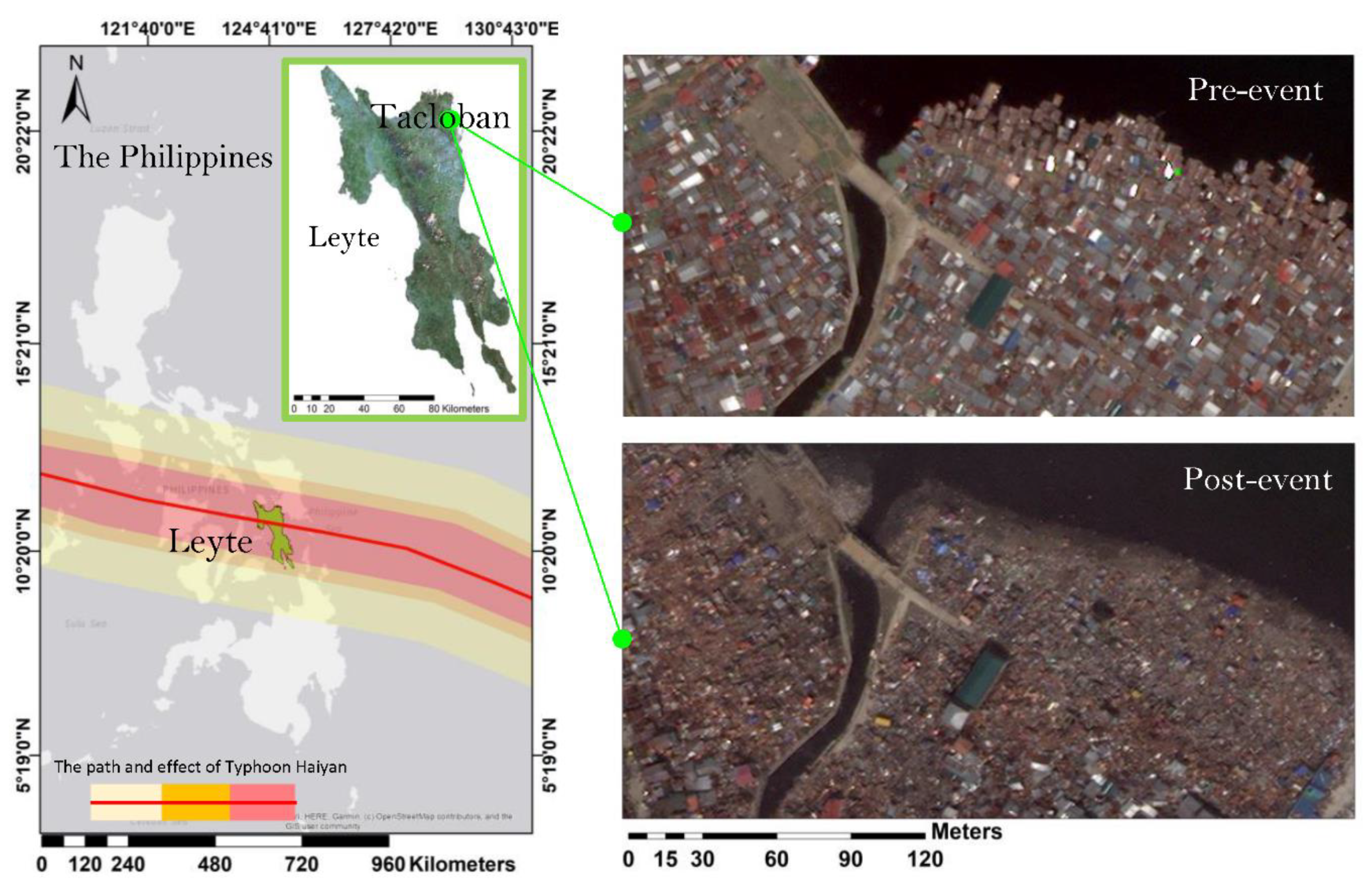
Leyte province, located in the Eastern Visayas, is the seventh largest island in the Philippines (Figure 1). With a population of approximately 250,000, Tacloban is the biggest city and the capital of Leyte, which in total houses ca. 1.7 million people. The region has a tropical climate with two slightly different rainfall patterns during a year. While most of Leyte island has an even annual rainfall distribution, some eastern parts have a pronounced maximum rainfall from November to January. Typhoon Haiyan (also known as Typhoon Yolanda in the region) passed over Leyte island close to Tacloban City on 8 November 2013. Tacloban was hit by the full force of the typhoon, which caused massive destruction in the city. A state of emergency was declared in Tacloban and the typhoon caused a storm surge of up to 5 m [44].
Since Leyte island is a tropical region and is covered by clouds most of the time, we first aimed at using Synthetic Aperture Radar (SAR) data. However, only Landsat images were available and found suitable for our study in the GEE data sets for the time of the disaster and recovery processes. Accordingly, atmospherically corrected surface reflectance Landsat 7 and 8 satellite images with 30 m spatial resolution were used to map the selected land cover types and implement the developed approach for post-disaster recovery assessment (Table 1). In total, 446 Landsat images were employed in this study. In particular the potential of big geospatial time-series data (i.e., Landsat 7 and 8 images) available on the cloud was used to generate the best-available-pixel image composites (explained in the methodology section) for the pre-disaster, event time, and post-disaster time steps over Leyte island to minimize/remove the cloud and shadow areas.
2.2. Reference Data and Land Cover Classes
We defined the land cover classes based on the local knowledge of the authors about the study area, and by considering the capacity/potential of the Landsat images (i.e., spatial and spectral resolutions) to identify different classes through field verification and visual interpretation of high-resolution satellite imagery acquired from various platforms (i.e., WorldView1-3, GeoEye 1, Pleiades) and images available from Google Earth Pro. We identified five land cover classes: forest/trees, built-up, crop land, water body, and other (i.e., non-tree vegetation, bare land, and debris/rubble) (Table 2), and the corresponding regions of interests (ROIs) were collected for training and testing of the classification method using the tools available within GEE.
2.3. Methods
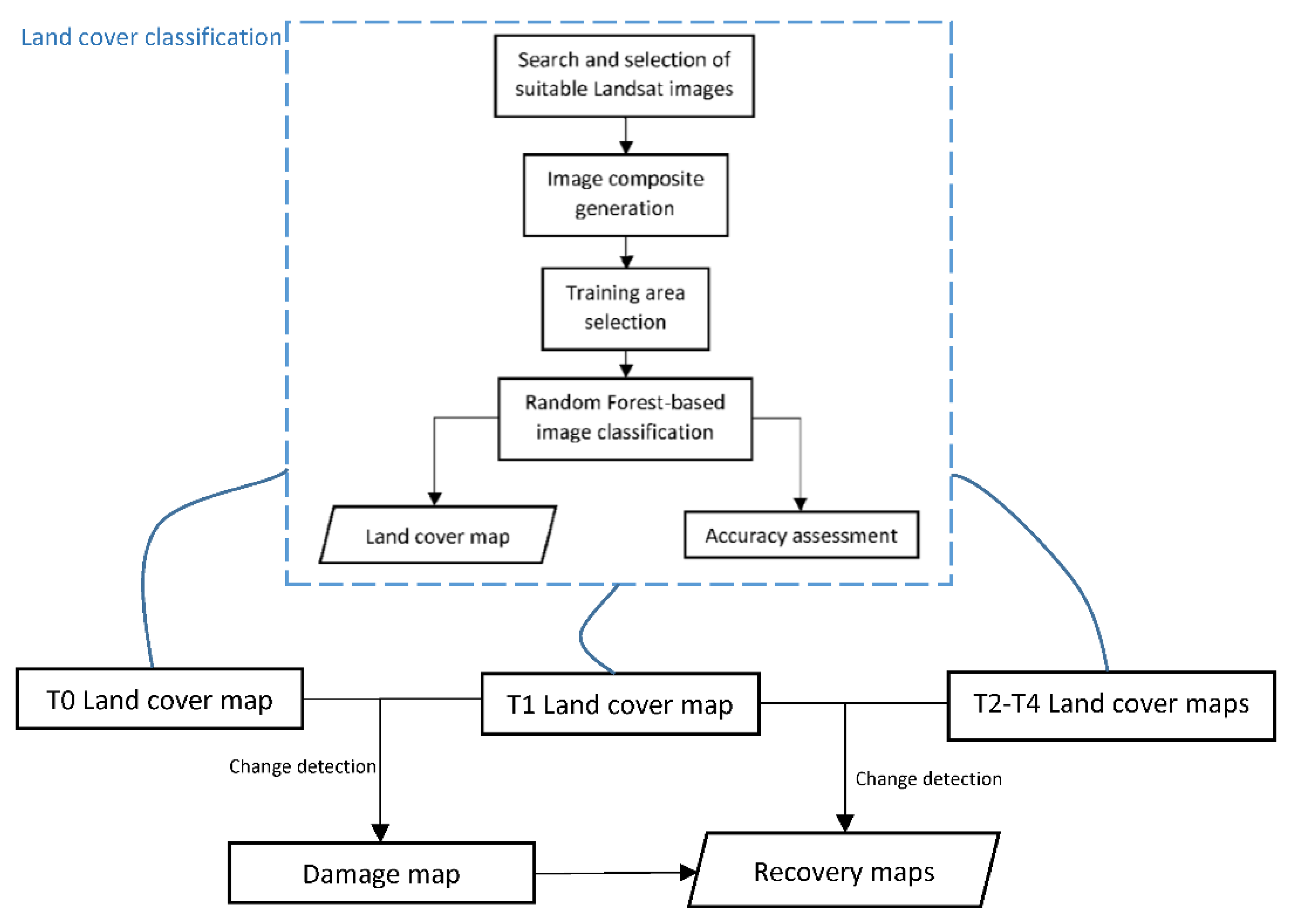
The developed approach for post-disaster recovery assessment has three main steps (Figure 2): (i) land cover classification of the pre-disaster, event time, and post-disaster images, (ii) change detection of pre-disaster and event time classified images to obtain the damage map, and (iii) change analysis of the post-disaster classified images and the damage map to obtain the recovery maps at T2–T4. Generating the land cover maps from the Landsat 7 and 8 satellite images with GEE consisted of three main stages: image composite generation, image classification, and accuracy assessment.
2.3.1. Image Composite Generation
We generated the best-available-pixel image composites for the T0–T4 time steps by extracting the best observations from several Landsat 7 and 8 images for our case study (Leyte island), using pixel-based image compositing within the GEE platform, and implemented using rule-based criteria such as dates of acquisition and exclusion of clouds and shadows [45,46,47,48]. To do so, we adapted a script within the GEE environment provided by De Alban et al. [43]. The generated Landsat image composites were exported for subsequent use in the image classification. The developed script needs user-defined inputs and parameters: the coordinates and extent of Leyte island, the number of years, starting and ending date range for the selected region (i.e., Leyte), the thresholds for cloud detection and masking (10% or less) and shadows (z-score = −1), and the image collection used, (i.e., Landsat 7 ETM+ and Landsat 8 OLI). Then the areas that were masked out in the previous step were filled by the median of the selected image pixels [43,49]. The scripts developed for this study are provided as supplementary materials in this paper.
In addition, we calculated five well-known indices from the Landsat composite images and added to the available Landsat bands to be used in the classification step as follows:
Normalized Difference Vegetation Index (NDVI; [50]) using Equation (1):
The Soil-Adjusted Total Vegetation Index (SATVI; [51]) using Equation (2):
Normalized Difference Tillage Index (NDTI; [56]) using Equation (5):
where Blue is the blue band, Red is the red band, NIR is the near-infrared band, SWIR1 is the shortwave infrared 1 band, and SWIR2 is the shortwave infrared 2 band of the Landsat image.
NDVI was shown to be a useful tool for distinguishing green vegetation areas from other land cover types; LSWI is for detecting water bodies and when combined with NDVI improves the performance of separating crop lands and forests [57]. SATVI, EVI, and NDTI have been shown to be effective tools for identifying forest and crop types from other land cover classes [43,58].
2.3.2. Image Classification
The final stacked/combined images for each time step consisted of seven Landsat bands (i.e., Blue, Green, Red, NIR, SWIR1, SWIR2, and TIR) and the computed indices (i.e., NDVI, EVI, SATVI, NDTI, and LSWI). The combined images were stored under the “Asset” tab of the GEE code editor platform to be later used for training and testing ROI selection/extraction.
We collected regions of interest (ROIs)/training areas from the images, using the tools within GEE in a way that each class had at least 40 polygons. These selections were based on field verifications and visual interpretations from high-resolution Google Earth Pro historical images and high-resolution satellite images acquired by different sensors (i.e., WorldView1-3, GeoEye1, Pleiades), and Landsat true- and false-color images to obtain final robust training and testing datasets. From the collected ROIs, 70% were randomly selected for training the classifier method and the rest were used for testing purposes. We used Random Forest, as an ensemble machine learning algorithm, to classify the images based on the collected training samples. Random Forest has been widely used in RS image processing for different applications [59], including land cover and land use classification [60,61], landslide detection [62], and hyperspectral image classification [63], due to providing efficient and accurate results. It is also one of the machine learning-based methods available and ready to use in GEE. This approach has also been used by other researchers and its ability to produce accurate classification results has been demonstrated [64,65,66,67]. In addition, Random Forest was selected as the best classifier among several advanced algorithms, including SVM and neural networks, for classifying hundreds of different real-world datasets [68].
Random Forest grows multiple decision trees on randomly selected training subsets. In addition, it takes the advantage of the bootstrapping approach to construct the decision trees from training samples and input variables at every node. The constructed numerous decision tress then go through the majority voting mechanism to obtain the final classification result. This strategy contributes to overcoming the limitations of single tree-based classifiers such as overfitting, and makes it less sensitive to noise. In the current study we executed Random Forest with 100 decision trees per class, a 0.5 fraction number to bag per tree, and 10 for the minimum size of a terminal node.
2.3.3. Accuracy Assessment
The overall user’s and producer’s accuracies were calculated for each time step classified maps (i.e., T0–T4) to assess the accuracy of the produced land cover classification results. A proportion of 30% of the collected ROIs for each class were selected using stratified random sampling for testing and computing the accuracy measures [51]. To do so, we adapted the code script used by De Alban et al. [43] and executed it within the GEE environment. Selecting the training and ground truth ROIs was challenging for some classes due to similarities between the land cover classes (e.g., crop land and vegetation classes). We tried to minimize the effect of these inaccuracies using different sources (e.g., very high-resolution satellite images) in selecting the ROIs. In addition, considering debris/rubble as the damaged area may cause inaccuracies, e.g., in the case of storm surge that may relocate/wash debris to other regions covering the intact built-up area [13].
2.3.4. Change Analysis
Final damage and recovery maps were generated based on the amount of change in the forest, built-up, and crop land classes. The changes were computed at the municipality level, and the damage map was generated by comparing the T0 and T1 land cover classification results; also, the recovery maps for each post-disaster time step (T2–T4) were computed by comparing the T1 and T2–T4 land cover classification results.
3. Results and Discussion
The proposed approach produced overall accuracies of 92.8%, 88.6%, 93.8%, 94.6%, and 89.0% for land cover classifications of the T0, T1, T2, T3, and T4 images, respectively (Table 3). In addition, Figure 3 shows the original true-color image composites and the results of the land cover classification for the T0–T4 time steps. Visual interpretation of the results and the high accuracy rates demonstrate the robustness of the approach and the Random Forest classifier for land cover classification for the defined classes in such a case study. However, the producer’s accuracy values of the built-up and the other (including non-tree vegetation, bare land, and debris) classes for T1 and T4 images were 76.5% and 75.4%, respectively, which shows the relatively high omission errors for those classes. Relocation of palm tree fronds by the typhoon made distinguishing trees, crop land, and other (including debris) classes more difficult for the event time, and resulted in the lowest overall accuracy of 88.6% for the T1 image classification. Furthermore, the generated composite images may still include cloud coverage. For example, the presence of clouds in the T4 image even after image composition generation resulted in some inaccuracies that produced the second-lowest overall accuracy of 89.0% among other images. The developed method produced accurate results in classifying built-up, water body, and forest/trees classes in most of the images.
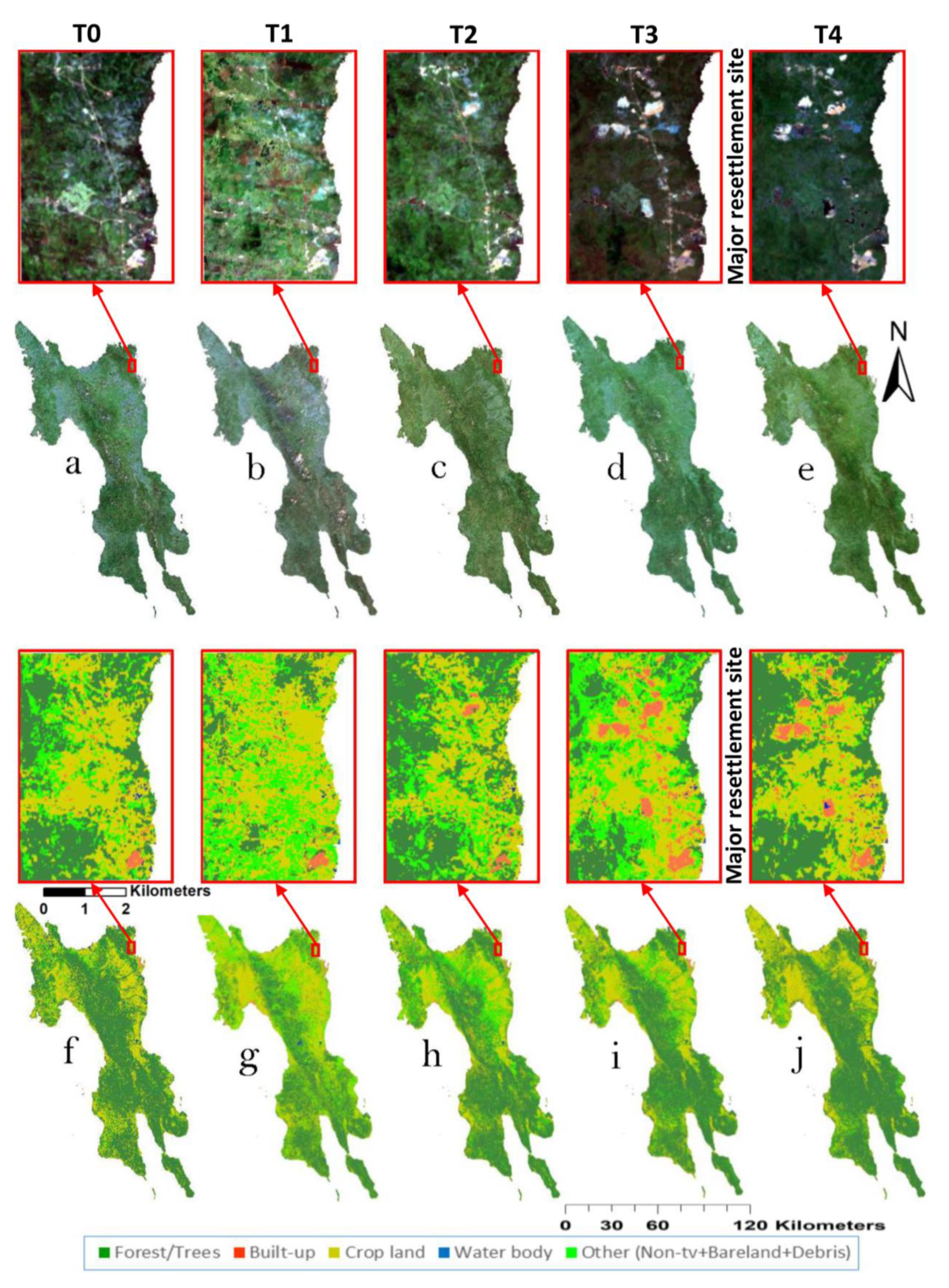
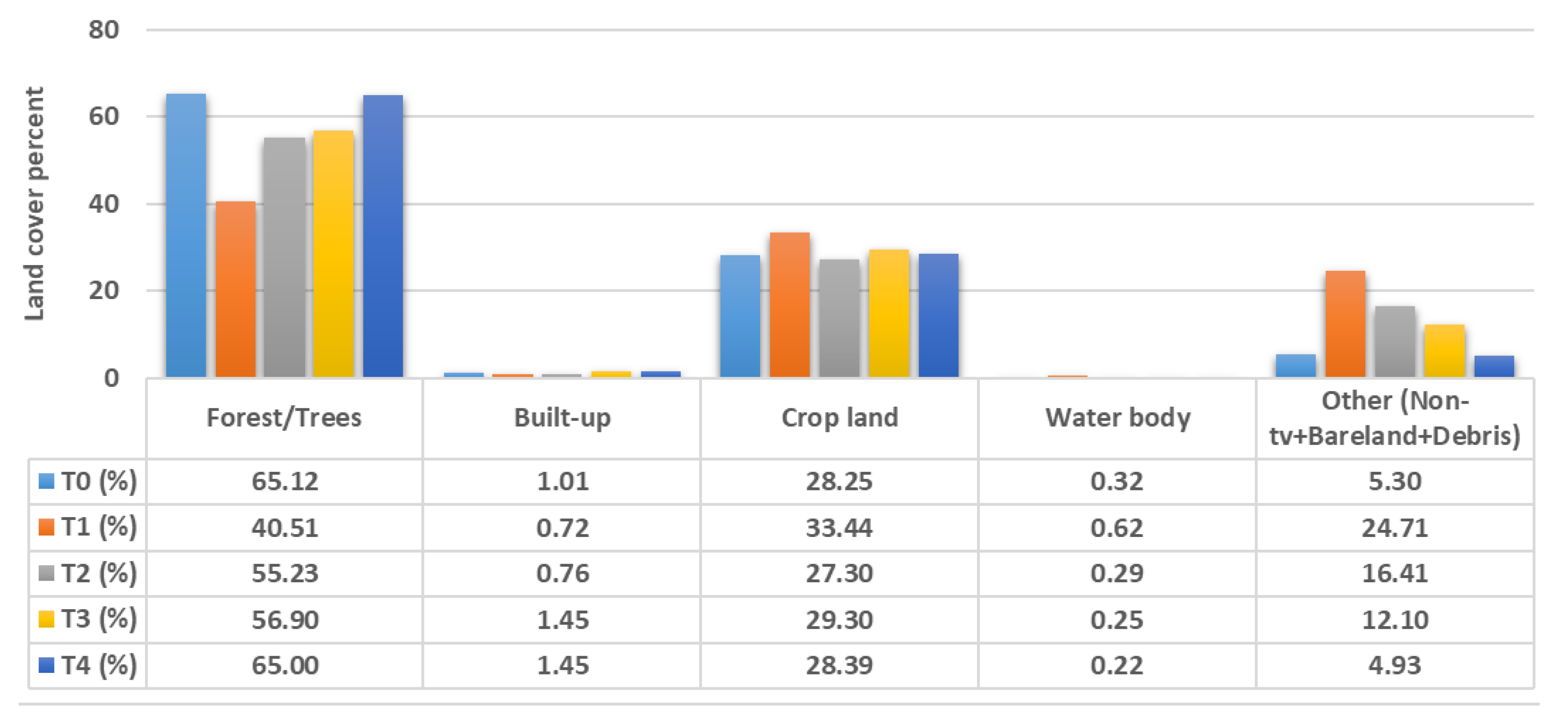
Figure 4 shows the land cover class change trends extracted from the T0 to T4 images. Typhoon Haiyan clearly had a significant impact on the forest/trees and built-up areas, reducing their coverage by about 40% and 30% from T0 to T1 images, respectively. The increase of the other class from T0 to T1 is mostly due to the debris and rubble caused by Haiyan and denuded trees, which led to an increase in non-tree vegetation coverage even in (formerly) forested areas. The storm surge during the typhoon resulted in the increase in water bodies in the T1 image. Monitoring three years after Typhoon Haiyan for Leyte island demonstrates that most of the land cover changes returned to their pre-disaster situation. However, there is an increase in the built-up class that is due to the construction of resettlement sites (as safe zones) mostly around the eastern coastal cities (e.g., Tacloban city—Figure 3).
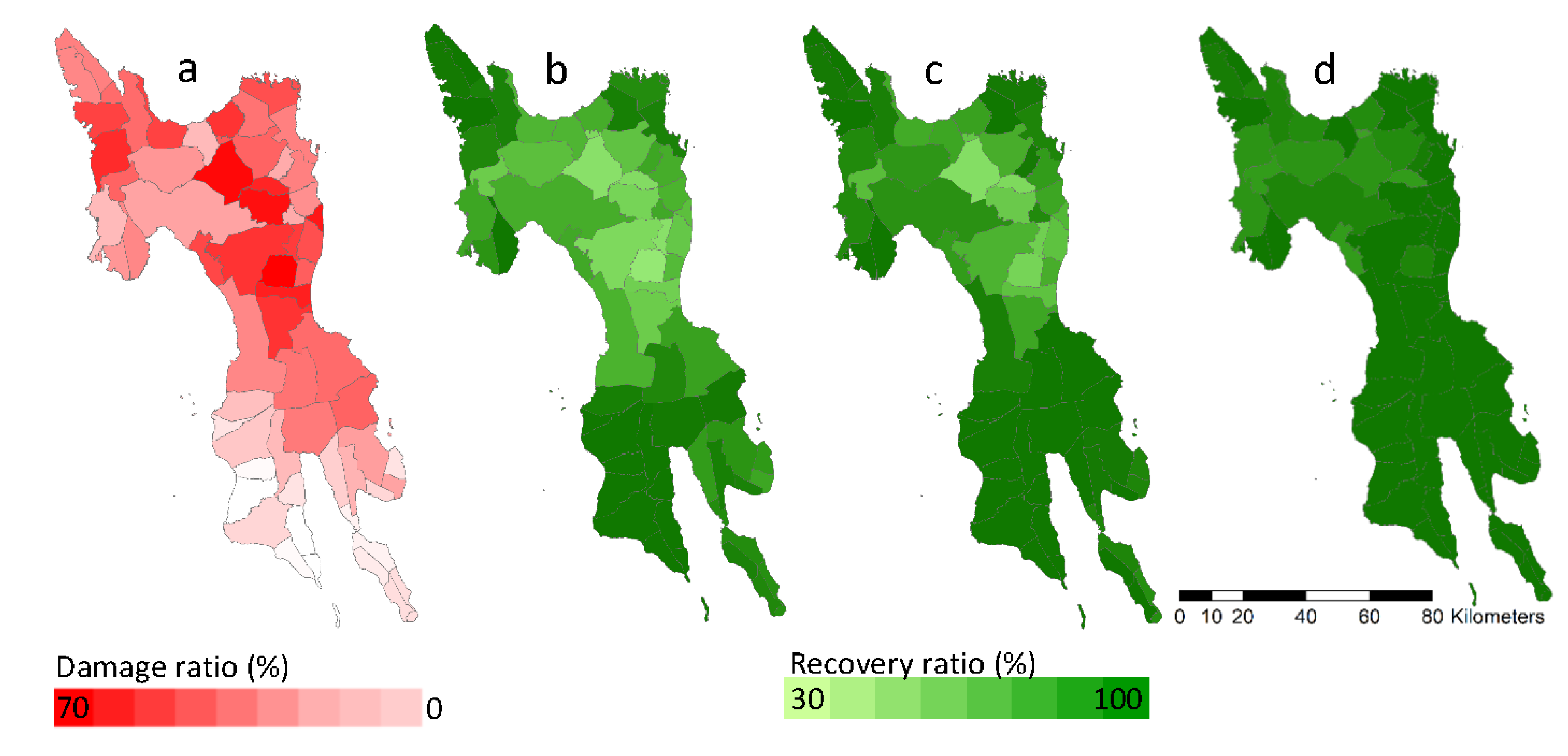
Figure 5 shows the damage and recovery maps for the post-Typhoon Haiyan situation generated at the municipality level for Leyte island. The damage map was produced based on the change analysis of the land cover classes for the T0 and T1 times, and recovery maps (RC) (i.e., RC1, RC2, and RC3) were produced based on change analysis of the damage map and the land cover classes of T2, T3, and T4 times, respectively.
In Figure 5, the darker red color shows more damage while, for the recovery maps, the darker green color shows a higher level of recovery. The most damaged/impacted municipalities are located in the center and northern part of the island. However, since Haiyan passed through the northern part of the island, the municipalities in the southern parts have the lowest damage ratios, close to zero. The most affected land cover classes were the forest/trees and built-up classes (Figure 4). Consequently, the municipalities with more forest/trees and built-up coverage compared to other land cover types have higher damage ratios. The change in the recovery maps (from RC1 to RC3) shows that the municipalities with more forest/tree coverage recovered more slowly than the others, and eventually, after a period of three years, most of the forest trees had recovered (RC3) (Figure 5d). Moreover, the results reported in a previous study [4] show almost the same pattern of recovery in terms of change in land cover classes at a small scale (i.e., Tacloban) in the post-Haiyan time. The only difference is in built-up class, where our study shows growth in built-up areas three years after Haiyan, while they reported that Tacloban city returned to almost the same level of built-up coverage four years after the disaster. This is mainly because their focus was on central urban areas of Tacloban, not including the northern part of Tacloban in their analysis, in which the primary resettlement sites for the period after Haiyan were built (Figure 3).
4. Discussion and Conclusions
The aim of this study was to assess the suitability of GEE for post-disaster recovery assessment for a large-scale region after Typhoon Haiyan, which hit Leyte island in the Philippines in 2013. We proposed an approach to monitor and quantify the recovery process using GEE, in particular with Landsat images, based on land cover classification and subsequent change analysis, and then producing municipality-based damage and recovery maps. The land cover classification results show the robustness of the employed approach, including image composite generation and Random Forest-based image classification. Furthermore, the change analysis and generated recovery maps clearly illustrate the damage and recovery processes during the selected time epochs, i.e., three time-steps for recovery assessment for three years after Haiyan. However, among the big geo dataset available in the platform and considering the time of Typhoon Haiyan (i.e., November 2013), we only found Landsat images suitable for this study. Hence, due to the limited spatial resolution of the data, detailed recovery analysis was not possible (e.g., extracting more land-use classes, such as building use and crop types). As also concluded by Sheykhmousa et al. [4], land cover maps can provide the main information for decision-makers to have an overview of the damage and reconstruction/recovery processes, which are critical in the early stages of recovery. However, a comprehensive recovery assessment needs more details that can be obtained using land use maps extracted from very high-resolution images. Little work has been done to date in damage and recovery mapping of the selected area, and none of this previous research investigated the entire Leyte island. In addition, the available studies that focused on some selected small areas were based on very high-resolution images with different class definitions. Hence, the validation is only based on the accuracy assessment of the land cover classification results. However, since GEE also allows to upload user images for processing, it might be used to upload a very high-resolution image for validation purposes.
Moreover, the change in types of crops and trees, or any detail about the recovered trees, can provide more information about the recovery process. For example, it is essential from the environmental and ecological points of view to understand whether the same trees that were denuded by the typhoon recovered, or whether the trees detected were newly planted after the disaster. More detailed information on the age of the trees can provide significant additional insights into the post-disaster recovery process.
In conclusion, further studies are needed to investigate the potential of the more recently available higher resolution optical and SAR images (Sentinel 1 and 2 images) for most of the case studies (i.e., disasters) that occurred after those platforms became operational. In addition, SAR data have been shown to be a useful tool for extracting land cover and use classes such as distinguishing different crop and tree types [43]. Hence, using higher resolution images and SAR data available in GEE will allow the researchers to detect damage to the crops, contribute to detecting changes in tree types, and extract more details for urban areas after a disaster [69,70,71].
Computer vision and image processing/classification methods deal with the actual image-based pixel values and try to classify them to achieve the best accuracies. However, in post-disaster remote sensing images, especially in water-related disasters, seeing actual damage and visually distinguishing damaged and intact areas is nearly impossible in some cases, as some intact areas are often buried under debris. Hence, assuming the debris area as the damaged class is not entirely correct, there is a need for further studies to identify the debris types (e.g., [13]) or use proxies for distinguishing between damaged and other classes [5] instead of only using direct image classification methods.
Evaluating the recovery process with more details (e.g., building use detection, crop type classification) and several time epochs at such a large scale, and providing municipality level recovery scores similar to those proposed in our study, can be further used for per-municipality resilience assessment at large scales, assuming that the speed of recovery is a proxy for evaluating resilience. However, it has been shown that this assumption is not correct for all cases, and further investigation is needed to clearly determine the relationship between the speed of the post-disaster recovery and resilience [6].
Although the Random Forest-based image classification produced a high accuracy rate, using more advanced methods (i.e., deep learning-based approaches) within the Google Earth API could help to improve the accuracy and would allow executing more advanced image classification and object detection tasks.
Supplementary Materials
Supplementary materials can be accessed at: https://www.mdpi.com/2076-3417/10/13/4574/s1.
Author Contributions
S.G. wrote the manuscript, designed and conducted the experiments. A.R.F. contributed to the design and developing the methodology, and conducting the experiments. N.K. and S.G. contributed to the conceptual design of the experiments, reviewed and revised the paper. All authors have read and agreed to the published version of the manuscript.
Funding
This research received no external funding.
Acknowledgments
We thank the anonymous reviewers for their insights and constructive comments, which helped to improve the paper.
Conflicts of Interest
The authors declare no conflict of interest.
References
- Mizutori, M.; Guha-Sapir, D. Economic Losses, Poverty and Disasters 1998–2017; United Nations Office for Disaster Risk Reduction: Geneva, Switzerland, 2017. [Google Scholar]
- Burton, C.; Mitchell, J.T.; Cutter, S.L. Evaluating post-Katrina recovery in Mississippi using repeat photography. Disasters 2011, 35, 488–509. [Google Scholar] [CrossRef]
- UNISDR. Sendai Framework for Disaster Risk Reduction 2015–2030. In Proceedings of the Third World Conference on Disaster Risk Reduction, Sendai, Japan, 14–18 March 2015; UNDRR: Sendai, Japan; pp. 1–25. [Google Scholar]
- Sheykhmousa, M.; Kerle, N.; Kuffer, M.; Ghaffarian, S. Post-disaster recovery assessment with machine learning-derived land cover and land use information. Remote Sens. 2019, 11, 1174. [Google Scholar] [CrossRef] [Green Version]
- Ghaffarian, S.; Kerle, N.; Filatova, T. Remote sensing-based proxies for urban disaster risk management and resilience: A review. Remote Sens. 2018, 10, 1760. [Google Scholar] [CrossRef] [Green Version]
- Kerle, N.; Ghaffarian, S.; Nawrotzki, R.; Leppert, G.; Lech, M. Evaluating resilience-centered development interventions with remote sensing. Remote Sens. 2019, 11, 2511. [Google Scholar] [CrossRef] [Green Version]
- Ebert, A.; Kerle, N.; Stein, A. Urban social vulnerability assessment with physical proxies and spatial metrics derived from air- and spaceborne imagery and GIS data. Nat. Hazards 2009, 48, 275–294. [Google Scholar] [CrossRef]
- Harb, M.M.; De Vecchi, D.; Dell’Acqua, F. Physical vulnerability proxies from remotes sensing: Reviewing, implementing and disseminating selected techniques. IEEE Geosci. Remote Sens. Mag. 2015, 3, 20–33. [Google Scholar] [CrossRef]
- Kerle, N.; Nex, F.; Gerke, M.; Duarte, D.; Vetrivel, A. UAV-based structural damage mapping: A review. ISPRS Int. J. Geo-Inf. 2019, 9, 14. [Google Scholar] [CrossRef] [Green Version]
- Vetrivel, A.; Kerle, N.; Gerke, M.; Nex, F.; Vosselman, G. Towards automated satellite image segmentation and classification for assessing disaster damage using data specific features with incremental learning. In Proceedings of the GEOBIA 2016, Solutions and Synergies, Enschede, The Netherlands, 14–16 September 2016. [Google Scholar]
- Vetrivel, A.; Gerke, M.; Kerle, N.; Vosselman, G. Identification of structurally damaged areas in airborne oblique images using a visual-bag-of-words approach. Remote Sens. 2016, 8, 231. [Google Scholar] [CrossRef] [Green Version]
- Nex, F.; Duarte, D.; Steenbeek, A.; Kerle, N. Towards real-time building damage mapping with low-cost UAV solutions. Remote Sens. 2019, 11, 287. [Google Scholar] [CrossRef] [Green Version]
- Ghaffarian, S.; Kerle, N. Towards post-disaster debris identification for precise damage and recovery assessments from UAV and satellite images. Int. Arch. Photogramm. Remote Sens. Spatial Inf. Sci. 2019, XLII-2/W13, 297–302. [Google Scholar] [CrossRef] [Green Version]
- Brown, D.; Platt, S.; Bevington, J.M. Disaster Recovery Indicators: Guidlines for Monitoring and Evaluation; CURBE, Cambridge University for Risk in the Built Environment, University of Cambridge: Cambridge, UK, 2010. [Google Scholar]
- Sutton, P.; Elvidge, C.; Ghosh, T. Estimation of gross domestic product at sub-national scales using night-time satellite imagery. Int. J. Ecol. Econ. Stat. 2007, 8, 5–21. [Google Scholar]
- Brown, D.; Saito, K.; Liu, M.; Spence, R.; So, E.; Ramage, M. The use of remotely sensed data and ground survey tools to assess damage and monitor early recovery following the 12.5.2008 Wenchuan earthquake in China. Bull. Earthq. Eng. 2011, 10, 741–764. [Google Scholar] [CrossRef]
- Costa Viera, A.; Kerle, N. Utility of Geo-Informatics for Disaster Risk Management: Linking Structural Damage Assessment, Recovery and Resilience; University of Twente: Enschede, The Netherlands, 2014. [Google Scholar]
- Hoshi, T.; Murao, O.; Yoshino, K.; Yamazaki, F.; Estrada, M. Post-disaster urban recovery monitoring in Pisco after the 2007 Peru earthquake using satellite image. J. Disaster Res. 2014, 9, 1059–1068. [Google Scholar] [CrossRef]
- Contreras, D.; Blaschke, T.; Tiede, D.; Jilge, M. Monitoring recovery after earthquakes through the integration of remote sensing, GIS, and ground observations: The case of L’aquila (Italy). Cart. Geog. Inf. Sci. 2016, 43, 115–133. [Google Scholar] [CrossRef]
- Kerle, N. Disasters: Risk assessment, management, and post-disaster studies using remote sensing. In Remote Sensing of Water Resources, Disasters, and Urban Studies; Taylor & Francis Group, LLC: Boca Raton, FL, USA, 2016. [Google Scholar]
- Chen, T.; Guestrin, C. Xgboost: A scalable tree boosting system. In Proceedings of the 22nd ACM SIGKDD International Conference on Knowledge Discovery and Data Mining; ACM: San Francisco, CA, USA, 2016; pp. 785–794. [Google Scholar]
- Georganos, S.; Grippa, T.; Vanhuysse, S.; Lennert, M.; Shimoni, M.; Wolff, E. Very high resolution object-based land use–land cover urban classification using extreme gradient boosting. IEEE Geosci. Remote Sens. Lett. 2018, 15, 607–611. [Google Scholar] [CrossRef] [Green Version]
- Duarte, D.; Nex, F.; Kerle, N.; Vosselman, G. Multi-resolution feature fusion for image classification of building damages with convolutional neural networks. Remote Sens. 2018, 10, 1636. [Google Scholar] [CrossRef] [Green Version]
- Nex, F.; Duarte, D.; Tonolo, F.G.; Kerle, N. Structural building damage detection with deep learning: Assessment of a state-of-the-art CNN in operational conditions. Remote Sens. 2019, 11, 2765. [Google Scholar] [CrossRef] [Green Version]
- Ghaffarian, S.; Kerle, N. Post-disaster recovery assessment using multi-temporal satellite images with a deep learning approach. In Proceedings of the 39th Earsel Conference, Salzburg, Austria, 1–4 July 2019. [Google Scholar]
- Ghaffarian, S.; Kerle, N.; Pasolli, E.; Jokar Arsanjani, J. Post-disaster building database updating using automated deep learning: An integration of pre-disaster OpenStreetMap and multi-temporal satellite data. Remote Sens. 2019, 11, 2427. [Google Scholar] [CrossRef] [Green Version]
- Ghaffarian, S.; Ghaffarian, S. Automatic building detection based on purposive FastICA (PFICA) algorithm using monocular high resolution Google Earth images. ISPRS J. Photogramm. Remote Sens. 2014, 97, 152–159. [Google Scholar] [CrossRef]
- Ghaffarian, S.; Ghaffarian, S. Automatic building detection based on supervised classification using high resolution Google Earth images. Int. Arch. Photogramm. Remote Sens. Spatial Inf. Sci. 2014, 40, 101. [Google Scholar] [CrossRef] [Green Version]
- Gorelick, N.; Hancher, M.; Dixon, M.; Ilyushchenko, S.; Thau, D.; Moore, R. Google Earth Engine: Planetary-scale geospatial analysis for everyone. Remote Sens. Environ. 2017, 202, 18–27. [Google Scholar] [CrossRef]
- Kumar, L.; Mutanga, O. Google Earth Engine applications since inception: Usage, trends, and potential. Remote Sens. 2018, 10, 1509. [Google Scholar] [CrossRef] [Green Version]
- Xie, Z.; Phinn, S.R.; Game, E.T.; Pannell, D.J.; Hobbs, R.J.; Briggs, P.R.; McDonald-Madden, E. Using Landsat observations (1988–2017) and Google Earth Engine to detect vegetation cover changes in rangelands—A first step towards identifying degraded lands for conservation. Remote Sens. Environ. 2019, 232, 111317. [Google Scholar] [CrossRef]
- Stromann, O.; Nascetti, A.; Yousif, O.; Ban, Y. Dimensionality reduction and feature selection for object-based land cover classification based on Sentinel-1 and Sentinel-2 time series using Google Earth Engine. Remote Sens. 2019, 12, 76. [Google Scholar] [CrossRef] [Green Version]
- Ge, Y.; Hu, S.; Ren, Z.; Jia, Y.; Wang, J.; Liu, M.; Zhang, D.; Zhao, W.; Luo, Y.; Fu, Y.; et al. Mapping annual land use changes in China’s poverty-stricken areas from 2013 to 2018. Remote Sens. Environ. 2019, 232, 111285. [Google Scholar] [CrossRef]
- Canty, M.J.; Nielsen, A.A.; Conradsen, K.; Skriver, H. Statistical analysis of changes in Sentinel-1 time series on the Google Earth Engine. Remote Sens. 2019, 12, 46. [Google Scholar] [CrossRef] [Green Version]
- Sidhu, N.; Pebesma, E.; Câmara, G. Using Google Earth Engine to detect land cover change: Singapore as a use case. Eur. J. Remote Sens. 2018, 51, 486–500. [Google Scholar] [CrossRef]
- Mahdianpari, M.; Salehi, B.; Mohammadimanesh, F.; Homayouni, S.; Gill, E. The first wetland inventory map of Newfoundland at a spatial resolution of 10 m using Sentinel-1 and Sentinel-2 data on the Google Earth Engine cloud computing platform. Remote Sens. 2018, 11, 43. [Google Scholar] [CrossRef] [Green Version]
- Wu, Q.; Lane, C.R.; Li, X.; Zhao, K.; Zhou, Y.; Clinton, N.; DeVries, B.; Golden, H.E.; Lang, M.W. Integrating lidar data and multi-temporal aerial imagery to map wetland inundation dynamics using Google Earth Engine. Remote Sens. Environ. 2019, 228, 1–13. [Google Scholar] [CrossRef] [Green Version]
- Zhou, B.; Okin, G.S.; Zhang, J. Leveraging Google Earth Engine (GEE) and machine learning algorithms to incorporate in situ measurement from different times for rangelands monitoring. Remote Sens. Environ. 2020, 236, 111521. [Google Scholar] [CrossRef]
- Xiong, J.; Thenkabail, P.S.; Gumma, M.K.; Teluguntla, P.; Poehnelt, J.; Congalton, R.G.; Yadav, K.; Thau, D. Automated cropland mapping of continental Africa using Google Earth Engine cloud computing. ISPRS J. Photogramm. Remote Sens. 2017, 126, 225–244. [Google Scholar] [CrossRef] [Green Version]
- Liu, C.-C.; Shieh, M.-C.; Ke, M.-S.; Wang, K.-H. Flood prevention and emergency response system powered by Google Earth Engine. Remote Sens. 2018, 10, 1283. [Google Scholar] [CrossRef] [Green Version]
- Sazib, N.; Mladenova, I.; Bolten, J. Leveraging the Google Earth Engine for drought assessment using global soil moisture data. Remote Sens. 2018, 10, 1265. [Google Scholar] [CrossRef] [PubMed] [Green Version]
- Crowley, M.A.; Cardille, J.A.; White, J.C.; Wulder, M.A. Generating intra-year metrics of wildfire progression using multiple open-access satellite data streams. Remote Sens. Environ. 2019, 232, 111295. [Google Scholar] [CrossRef]
- De Alban, J.D.T.; Connette, G.M.; Oswald, P.; Webb, E.L. Combined Landsat and L-band SAR data improves land cover classification and change detection in dynamic tropical landscapes. Remote Sens. 2018, 10, 306. [Google Scholar] [CrossRef] [Green Version]
- NDRRMC. Final Reports for Effects of Typhoon Yolanda (Haiyan); National Disaster Risk Reduction and Management Council of Philippines: Quezon City, Philippines, 2014. [Google Scholar]
- Hansen, M.C.; Loveland, T.R. A review of large area monitoring of land cover change using Landsat data. Remote Sens. Environ. 2012, 122, 66–74. [Google Scholar] [CrossRef]
- Wulder, M.A.; Masek, J.G.; Cohen, W.B.; Loveland, T.R.; Woodcock, C.E. Opening the archive: How free data has enabled the science and monitoring promise of Landsat. Remote Sens. Environ. 2012, 122, 2–10. [Google Scholar] [CrossRef]
- Griffiths, P.; Linden, S.v.d.; Kuemmerle, T.; Hostert, P. A pixel-based Landsat compositing algorithm for large area land cover mapping. IEEE J. Sel. Top. Appl. Earth Observ. Remote Sens. 2013, 6, 2088–2101. [Google Scholar] [CrossRef]
- White, J.C.; Wulder, M.A.; Hobart, G.W.; Luther, J.E.; Hermosilla, T.; Griffiths, P.; Coops, N.C.; Hall, R.J.; Hostert, P.; Dyk, A.; et al. Pixel-based image compositing for large-area dense time series applications and science. Can. J. Remote Sens. 2014, 40, 192–212. [Google Scholar] [CrossRef] [Green Version]
- Reductions, G.D.I. Introduction to Google Earth Engine. Available online: Https://developers.Google.Com/earthengine/ (accessed on 10 January 2020).
- Tucker, C.J. Red and photographic infrared linear combinations for monitoring vegetation. Remote Sens. Environ. 1979, 8, 127–150. [Google Scholar] [CrossRef] [Green Version]
- Marsett, R.C.; Qi, J.; Heilman, P.; Biedenbender, S.H.; Carolyn Watson, M.; Amer, S.; Weltz, M.; Goodrich, D.; Marsett, R. Remote sensing for grassland management in the arid Southwest. Rangel. Ecol. Manag. 2006, 59, 530–540. [Google Scholar] [CrossRef]
- Huete, A.R.; Liu, H.Q.; Batchily, K.; van Leeuwen, W. A comparison of vegetation indices over a global set of TM images for EOS-MODIS. Remote Sens. Environ. 1997, 59, 440–451. [Google Scholar] [CrossRef]
- Huete, A.; Didan, K.; Miura, T.; Rodriguez, E.P.; Gao, X.; Ferreira, L.G. Overview of the radiometric and biophysical performance of the modis vegetation indices. Remote Sens. Environ. 2002, 83, 195–213. [Google Scholar] [CrossRef]
- Gao, B.-c. NDWI—A normalized difference water index for remote sensing of vegetation liquid water from space. Remote Sens. Environ. 1996, 58, 257–266. [Google Scholar] [CrossRef]
- Jurgens, C. The modified normalized difference vegetation index (MNDVI) a new index to determine frost damages in agriculture based on landsat tm data. Int. J. Remote Sens. 1997, 18, 3583–3594. [Google Scholar] [CrossRef]
- Van Deventer, A.P.; Ward, A.D.; Gowda, P.H.; Lyon, J.G. Using thematic mapper data to identify contrasting soil plains and tillage practices. Photogramm. Eng. Remote Sens. 1997, 63, 87–93. [Google Scholar]
- Xiao, X.; Boles, S.; Frolking, S.; Salas, W.; Moore, B.; Li, C.; He, L.; Zhao, R. Landscape-scale characterization of cropland in China using vegetation and Landsat TM images. Int. J. Remote Sens. 2002, 23, 3579–3594. [Google Scholar] [CrossRef]
- Torbick, N.; Ledoux, L.; Salas, W.; Zhao, M. Regional mapping of plantation extent using multisensor imagery. Remote Sens. 2016, 8, 236. [Google Scholar] [CrossRef] [Green Version]
- Belgiu, M.; Drăguţ, L. Random forest in remote sensing: A review of applications and future directions. ISPRS J. Photogramm. Remote Sens. 2016, 114, 24–31. [Google Scholar] [CrossRef]
- Gislason, P.O.; Benediktsson, J.A.; Sveinsson, J.R. Random forests for land cover classification. Patt. Recog. Lett. 2006, 27, 294–300. [Google Scholar] [CrossRef]
- Abdi, A.M. Land cover and land use classification performance of machine learning algorithms in a boreal landscape using Sentinel-2 data. GISci. Remote Sens. 2019, 57, 1–20. [Google Scholar] [CrossRef] [Green Version]
- Stumpf, A.; Kerle, N. Object-oriented mapping of landslides using random forests. Remote Sens. Environ. 2011, 115, 2564–2577. [Google Scholar] [CrossRef]
- Ham, J.; Yangchi, C.; Crawford, M.M.; Ghosh, J. Investigation of the random forest framework for classification of hyperspectral data. IEEE Tran. Geosci. Remote Sens. 2005, 43, 492–501. [Google Scholar] [CrossRef] [Green Version]
- Shelestov, A.; Lavreniuk, M.; Kussul, N.; Novikov, A.; Skakun, S. Exploring Google Earth Engine platform for big data processing: Classification of multi-temporal satellite imagery for crop mapping. Front. Earth Sci. 2017, 5, 4225. [Google Scholar] [CrossRef] [Green Version]
- Teluguntla, P.; Thenkabail, P.S.; Oliphant, A.; Xiong, J.; Gumma, M.K.; Congalton, R.G.; Yadav, K.; Huete, A. A 30-m Landsat-derived cropland extent product of Australia and China using random forest machine learning algorithm on Google Earth Engine cloud computing platform. ISPRS J. Photogramm. Remote Sens. 2018, 144, 325–340. [Google Scholar] [CrossRef]
- Kelley, L.C.; Pitcher, L.; Bacon, C. Using Google Earth Engine to map complex shade-grown coffee landscapes in northern Nicaragua. Remote Sens. 2018, 10, 952. [Google Scholar] [CrossRef] [Green Version]
- Oliphant, A.J.; Thenkabail, P.S.; Teluguntla, P.; Xiong, J.; Gumma, M.K.; Congalton, R.G.; Yadav, K. Mapping cropland extent of Southeast and Northeast Asia using multi-year time-series Landsat 30-m data using a random forest classifier on the Google Earth Engine cloud. Int. J. Appl. Earth Obs. Geoinf. 2019, 81, 110–124. [Google Scholar] [CrossRef]
- Fernández-Delgado, M.; Cernadas, E.; Barro, S.; Amorim, D. Do We Need Hundreds of Classifiers to Solve Real World Classification Problems? J. Mach. Learn. Res. 2014, 15, 3133–3181. [Google Scholar]
- Dadhich, G.; Miyazaki, H.; Babel, M. Applications of Sentinel-1 synthetic aperture radar imagery for floods damage assessment: A case study of Nakhon Si Thammarat, Thailand. Int. Arch. Photogramm. Remote Sens. Spatial Inf. Sci. 2019, 4213, 1927–1931. [Google Scholar] [CrossRef] [Green Version]
- Phan, A.; Ha, D.N.; Man, C.D.; Nguyen, T.T.; Bui, H.Q.; Nguyen, T.T.N. Rapid assessment of flood inundation and damaged rice area in red river delta from Aentinel 1A imagery. Remote Sens. 2019, 11, 2034. [Google Scholar] [CrossRef] [Green Version]
- Bell, J.; Gebremichael, E.; Molthan, A.; Schultz, L.; Meyer, F.; Shrestha, S. Synthetic Aperture Radar and Optical Remote Sensing of Crop Damage Attributed to Severe Weather in the Central United States. In Proceedings of the IGARSS 2019, Yokohama, Japan, 28 July–2 August 2019; IEEE: Yokohama, Japan; pp. 9938–9941. [Google Scholar]
Figure 1.
An overview of the Philippines showing the path of Typhoon Haiyan and the location of Leyte island. Pre-event image and an image acquired three days after the disaster for Tacloban.
Figure 1.
An overview of the Philippines showing the path of Typhoon Haiyan and the location of Leyte island. Pre-event image and an image acquired three days after the disaster for Tacloban.

Figure 2.
The proposed framework for post-disaster recovery monitoring.

Figure 3.
(a–e) Landsat image composites acquired over Leyte island for T0–T4 times, respectively, (f–j) land cover classification maps produced with GEE for T0–T4 times, respectively. Red rectangles show the status of the relocation site (northern part of Tacloban) for T0–T4 times. Non-tv—Non-tree vegetation.

Figure 4.
Per class land cover percentage for Leyte island for T0–T4. Non-tv—Non-tree vegetation.

Figure 5.
(a) Municipality level damage map for T1 and (b–d) the recovery maps for T2–T4 times after Typhoon Haiyan for Leyte island, respectively.
Figure 5.
(a) Municipality level damage map for T1 and (b–d) the recovery maps for T2–T4 times after Typhoon Haiyan for Leyte island, respectively.


Table 1.
Satellite images used in this study.
| ID | Timeline | Acquisition Dates | Number of Images Collected | Satellite Platforms | Spatial Resolution |
|---|---|---|---|---|---|
| T0 | Before Haiyan | 2013-05-01 to 2013-10-28 | 68 | Landsat 7 ETM+ and Landsat 8 OLI | 30 m |
| T1 | Event time | 2013-11-10 to 2014-03-31 | 56 | ||
| T2 | Post-Haiyan 1 | 2014-06-01 to 2014-12-30 | 104 | ||
| T3 | Post-Haiyan 2 | 2015-06-01 to 2015-12-30 | 109 | ||
| T4 | Post-Haiyan 3 | 2016-06-01 to 2016-12-30 | 109 |
Table 2.
Description of the selected land cover classes.
| ID | Land Cover Class | Description |
|---|---|---|
| 1 | Forest/Trees | All types of trees (e.g., forest, palm and banana), tree canopy coverage >30% |
| 2 | Built-up | Any type of developed lands such as buildings, roads, impervious surfaces |
| 3 | Crop land | Agricultural fields with any non-tree crop type plantation |
| 4 | Water body | Bodies of water including lakes, oceans, rivers and flooded areas |
| 5 | Other | All other land cover classes (i.e., non-tree vegetation, bare land, rubble and debris) |
Table 3.
The land cover classification accuracies for T0, T1, T2, T3, and T4 time epochs for Leyte island. PA—producer’s accuracy; UA—user’s accuracy; OA—overall accuracy; Non-tv—Non-tree vegetation.
Table 3.
The land cover classification accuracies for T0, T1, T2, T3, and T4 time epochs for Leyte island. PA—producer’s accuracy; UA—user’s accuracy; OA—overall accuracy; Non-tv—Non-tree vegetation.
| Time/Class | Trees | Built-Up | Crop Land | Water Body | Other (Non-tv, Bare Land, Debris) | |
|---|---|---|---|---|---|---|
| Pre-disaster (T0) | UA(%) | 90.7 | 100 | 93.0 | 100 | 86.7 |
| PA(%) | 87.3 | 100 | 84.6 | 100 | 85.8 | |
| OA(%) | 92.8 | |||||
| Event time (T1) | UA(%) | 98.4 | 94.8 | 85.1 | 100 | 71.9 |
| PA(%) | 84.1 | 100 | 84.9 | 100 | 76.5 | |
| OA(%) | 88.6 | |||||
| Post-disaster (T2) | UA(%) | 96.4 | 89.1 | 90.6 | 99.9 | 90.3 |
| PA(%) | 88.4 | 95.7 | 90.6 | 99.8 | 96.4 | |
| OA(%) | 93.8 | |||||
| Post-disaster (T3) | UA(%) | 95.7 | 98.5 | 84.8 | 100 | 86.5 |
| PA(%) | 93.1 | 97.8 | 98.7 | 100 | 91.3 | |
| OA(%) | 94.6 | |||||
| Post-disaster (T4) | UA(%) | 90.1 | 81.0 | 86.3 | 99.5 | 86.7 |
| PA(%) | 96.6 | 75.4 | 93.3 | 99.9 | 82.6 | |
| OA(%) | 89.0 | |||||
© 2020 by the authors. Licensee MDPI, Basel, Switzerland. This article is an open access article distributed under the terms and conditions of the Creative Commons Attribution (CC BY) license (http://creativecommons.org/licenses/by/4.0/).
Share and Cite
MDPI and ACS Style
Ghaffarian, S.; Rezaie Farhadabad, A.; Kerle, N. Post-Disaster Recovery Monitoring with Google Earth Engine. Appl. Sci. 2020, 10, 4574. https://doi.org/10.3390/app10134574
AMA Style
Ghaffarian S, Rezaie Farhadabad A, Kerle N. Post-Disaster Recovery Monitoring with Google Earth Engine. Applied Sciences. 2020; 10(13):4574. https://doi.org/10.3390/app10134574
Chicago/Turabian StyleGhaffarian, Saman, Ali Rezaie Farhadabad, and Norman Kerle. 2020. "Post-Disaster Recovery Monitoring with Google Earth Engine" Applied Sciences 10, no. 13: 4574. https://doi.org/10.3390/app10134574
Note that from the first issue of 2016, this journal uses article numbers instead of page numbers. See further details here.